The Gamma-Ray Burst Hubble Diagram and its Implications for Cosmology

Abstract

In this paper, we continue to build support for the proposal to use gamma-ray bursts (GRBs) as standard candles in constructing the Hubble Diagram at redshifts beyond the current reach of Type Ia supernova observations. We confirm that correlations among certain spectral and lightcurve features can indeed be used as luminosity indicators, and demonstrate from the most up-to-date GRB sample appropriate for this work that the $\Lambda$CDM model optimized with these data is characterized by parameter values consistent with those in the concordance model. Specifically, we find that $(\Omega_{m},\Omega_{\Lambda})\approx(0.25_{-0.06}^{+0.05},0.75_{-0.05}^{+0.06})$, which are consistent, to within $1\sigma$, with $(0.29,0.71)$ obtained from the 9-yr WMAP data. We also carry out a comparative analysis between $\Lambda$CDM and the $R_{\rm h}=ct$ Universe and find that the optimal $\Lambda$CDM model fits the GRB Hubble Diagram with a reduced $\chi^{2}_{\rm dof}\approx 2.26$, whereas the fit using $R_{\rm h}=ct$ results in a $\chi^{2}_{\rm dof}\approx 2.14$. In both cases, about $20\%$ of the events lie at least $2\sigma$ away from the best-fit curves, suggesting that either some contamination by non-standard GRB luminosities is unavoidable, or that the errors and intrinsic scatter associated with the data are being underestimated. With these optimized fits, we use three statistical tools—the Akaike Information Criterion (AIC), the Kullback Information Criterion (KIC), and the Bayes Information Criterion (BIC)—to show that, based on the GRB Hubble Diagram, the likelihood of $R_{\rm h}=ct$ being closer to the correct model is $\sim 85-96\%$, compared to $\sim 4-15\%$ for $\Lambda$CDM.

1 Introduction

For a given class of sources whose luminosity is accurately known, one may construct a Hubble Diagram (HD) from the measurement of their distance versus redshift. Such a relationship can be a powerful tool for probing the cosmological expansion of the Universe, but only if these sources truly function as standard candles. The cosmic evolution depends critically on its constituents, so measuring distances over a broad range of redshifts can in principle place meaningful constraints on the assumed cosmology. The discovery of dark energy was made using this method, in which the sources—Type Ia supernovae—are transient, though with a well-defined luminosity versus color and light-curve shape relationships (Riess et al. 1998; Perlmutter et al. 1998, 1999; Garnavich et al. 1998; Schmidt et al. 1998). Of course, one must also assume that the power of distant explosions can be standardized against those seen at much lower redshifts.

The use of Type Ia SNe has been quite impressive, so one may wonder why there would be a need to seek other kinds of standard candle. But the reality is that several important limitations mitigate the overall impact of supernova studies. For example, even excellent space-based platforms, such as SNAP (Scholl et al. 2004), cannot observe these events at redshifts $\gtrsim 1.8$. And this is quite limiting because much of the most interesting evolution of the Universe occurred well before this epoch. In addition, the determination of the supernova luminosity cannot be carried out independently of the assumed cosmology, so the Type Ia SN data tend to be compliant to the adopted expansion scenario (Melia 2012a). The fact that so-called “nuisance” parameters associated with the data need to be optimized along with the variables in the model itself weakens any comparative analysis between competing cosmologies. There is therefore much more to learn about the Universe’s history than one can infer from Type Ia SNe alone.

In recent years, several other classes of source have been proposed as possible standard candles in their own right. Most recently, the discovery that high-$z$ quasars appear to be accreting at close to their Eddington limit (see, e.g., Willott et al. 2010), has made it possible to begin using them to construct an HD at redshifts beyond $\sim 6$ (Melia 2012b). It has also been suggested that Gamma-ray Bursts (GRBs) may be suitable for constructing an HD at intermediate redshifts, $1\lesssim z\lesssim 6$, between the Type Ia SN and high-$z$ quasar regions.

The possible use of GRBs as standard candles started to become reality after Norris et al. (2000) found a tight correlation between the burst luminosity $L$ and the spectral lag $\tau_{\rm lag}$. Some other GRB luminosity indicators have been widely discussed in the literature. Amati et al. (2002) discovered a relationship between the isotropic equivalent gamma-ray energy $(E_{\gamma,{\rm iso}})$ and the burst frame peak energy in the GRB spectrum $(E_{\rm p})$, but the relation may be the result of selection effects (see, e.g., Kocevski 2012; Collazzi et al. 2012). Similarly, the isotropic peak luminosity $(L_{\gamma,{\rm iso}})$ is also found to be correlated with $E_{\rm p}$ in the burst frame (Schaefer 2003a; Wei & Gao 2003; Yonetoku et al. 2004). Ghirlanda et al. (2004a) replaced $E_{\gamma,{\rm iso}}$ with collimation-corrected gamma-ray energy $(E_{\gamma})$, and claimed a tighter correlation between $E_{\rm p}$ and $E_{\gamma}$. Since $E_{\gamma}=E_{\gamma,{\rm iso}}(1-\cos\theta)$, where $\theta$ is the jet half-opening angle, one may reliably estimate the isotropically equivalent energy $E_{\gamma,{\rm iso}}$ and use this to infer a distance. Liang & Zhang (2005) introduced the concept of optical temporal break time $t_{\rm b}$, and discovered a strong dependence of $E_{\gamma,{\rm iso}}$ on $E_{\rm p}$ and $t_{\rm b}$ without imposing any theoretical models.

Earlier, Schaefer (2003b) had constructed the first GRB HD based on nine events using two luminosity indicators, and this was followed by Bloom et al. (2003a), who published a GRB HD with 16 bursts, assuming that the burst energy is a constant after correcting for the beam angle. Some authors attempted to show the HD for an observed GRB sample plotted against a theoretical HD calculated using the same cosmological parameters (e.g., Dai et al. 2004; Liang & Zhang 2005; Xu et al. 2005). These and other attempts at constructing a GRB HD were made with only a small fraction of the available data, using only one or two luminosity indicators. Unfortunately, all of them had error bars that were too large to provide useful constraints on cosmology. Schaefer (2007) made use of five luminosity indicators and successfully constructed a GRB HD with 69 events.

The feasibility of using this method became better grounded when Dai et al. (2004) used the correlation found by Ghirlanda et al. (2004a) to place tight constraints on the cosmological parameters. Because of the current poor information on low-$z$ GRBs, the Ghirlanda relation necessarily depends on the assumed cosmology. Other authors attempted to circumvent the circularity problem by using a less model-dependent approach (Ghirlanda et al. 2004b, 2006; Firmani et al. 2005; Xu et al. 2005; Liang & Zhang 2005, 2006; Wang & Dai 2006; Su et al. 2006; Li et al. 2008; Qi et al. 2008a, 2008b; Liang et al. 2008; Wang et al. 2011). In the end, however, as is also true for Type Ia SNe, the correlation must still be recalibrated for each different model because the best-fit correlation depends on the cosmology adopted to derive the burst luminosities.

Of course, even with the emergence of more precise luminosity indicators, one must still deal with several significant challenges when trying to use GRBs to construct an HD. The luminosity of these bursts, calculated assuming isotropy, spans about 4 orders of magnitude (Frail et al. 2001). However, there is strong observational evidence (e.g., the achromatic break in the afterglow lightcurve) that the burst emission is collimated into a jet with the aforementioned aperture angle $\theta$ (Levinson & Eichler 1993; Rhoads 1997; Sari et al. 1999; Fruchter et al. 1999). When one corrects for the collimation factor $(1-\cos\theta)$, the gamma-ray energy tends to cluster around $E_{\gamma}\sim 10^{51}$ ergs, but the dispersion ($\sim 0.5$ dex) is still too large for these measurements to be used for cosmological purposes. For example, Wang et al. (2011) found that the updated $\tau_{\rm lag}-L$ correlation has a large intrinsic scatter. And Lu et al. (2012) presented a time-resolved $E_{\rm p}-L_{\gamma,{\rm iso}}$ correlation analysis and showed that the scatter of the correlation is comparable to that of the time-integrated relation. So in the end, theses luminosity correlations may also not be suitable for cosmological purposes. This is why much effort has been expended since 2004 in finding other indicators from the GRB spectrum that provide more precise constraints on the luminosity.

One useful application of these ideas involves the use of $E_{\rm p}$ and $t_{\rm b}$ (the so-called jet break time) as a measure of $\theta$ to determine $E_{\gamma,{\rm iso}}$ (Liang & Zhang 2005). In this paper, we will follow this approach with two distinct goals in mind. First, several new GRB events have been detected in recent years that have spectral and lightcurve features (such as $t_{\rm b}$) with sufficient quality to help improve the previously assembled correlations. Second, and foremost, we wish to use this relatively new probe of the Universe’s expansion to directly test the $R_{\rm h}=ct$ Universe (Melia 2007; Melia & Shevchuk 2012) against the data and to see how its predictions compare with those of the $\Lambda$CDM cosmology.

The $R_{\rm h}=ct$ Universe is a Friedmann-Robertson-Walker cosmology that strictly adheres to the simultaneous requirements of both the Cosmological principle and Weyl’s postulate. Whereas $\Lambda$CDM guesses the constituents of the Universe and their equation of state, and then predicts the expansion rate as a function of time, $R_{\rm h}=ct$ acknowledges the fact that no matter what these constituents are, the total energy density in the Universe gives rise to a gravitational horizon coincident with the better known Hubble radius. But because this radius is therefore a proper distance, the application of Weyl’s postulate forces it to always equal $ct$. Thus, on every time slice, the energy density must partition itself among its various constituents in such a way as to always adhere to this constraint, which also guarantees that the expansion rate be constant in time. As we shall see, with all its complexity, $\Lambda$CDM actually mimics the $R_{\rm h}=ct$ Universe when its free parameters are optimized to produce a best fit to the cosmological data.

In the next section, we will describe the data we will use and our method of analysis. We will then first assemble the GRB HD in the context of the standard model, $\Lambda$CDM, and demonstrate that the best-fit parameters obtained by fitting its predicted luminosity distance to the GRB observations very closely mirror those obtained through the analysis of Type Ia SNe. In § 4, we will introduce the $R_{\rm h}=ct$ Universe and provide a brief overview of its current status as a viable cosmology. We will then construct the GRB HD for this expansion scenario, which is much easier to do than for $\Lambda$CDM because the former has only one free parameter—the Hubble constant $H_{0}$. Finally, we will directly compare the results of our fits to the data with both $\Lambda$CDM and $R_{\rm h}=ct$.

2 Observational data and Methodology

Our GRB sample includes 33 bursts with a measurement of the redshift z, the spectral peak energy $E_{\rm p}$, and the jet break time $t_{\rm b}$ seen in the optical afterglow. In assembling this sample, we required that the members have an independent z, that a spectral fit be available, and that a jet-break characteristic be present in the optical band lightcurve. Note that in order to preserve homogeneity, we did not include those bursts whose afterglow break times were observed in the radio band (e.g., GRB 970508) or in the X-ray band (e.g., GRBs 050318, 050505, 051022, 060124, 060210) but were not seen in the optical band. We also excluded those bursts whose z or $E_{\rm p}$ were not directly measured. For example, because of the narrowness of the Swift/BAT band, the spectrum of GRB 050904 can be described using a simple power law (Tagliaferri et al. 2005), so we do not know the real $E_{\rm p}$. Some bursts with reported z and $E_{\rm p}$ were also not included for a variety of reasons: GRB 050820A does not have a well measured $t_{\rm b}$; there is only one observed datum in the last decay phase of its optical lightcurve (see Fig. 4 of Cenko et al. 2006). The optical lightcurve of GRB 060418 is characterized by an initial sharp rise, peaking at 100 $-$ 200 s, with a subsequent power-law decay (Molinari et al. 2007). GRB 060418 does not have a jet-break characteristic. Racusin et al. (2008) found that the observed afterglow of GRB 080319B can be interpreted using a two-component jet model, so this burst may not be a “Gold” jet-break burst. GRB 090323, GRB 090328, and GRB 090902B do not have clear jet-break characteristics in their optical band (see Figs. 2, 4, and 6 of Cenko et al. 2011). GRB 090926A is one of the brightest long bursts detected by the GBM and LAT instruments on Fermi with high-energy events up to $\sim$ 20 GeV. This burst shows an extra hard component in its integrated spectrum, whose break energy is around 1.4 GeV. The integrated spectrum can be well fitted by two Band functions (Ackermann et al. 2011), so the real $E_{\rm p}$ is confusing.

In summary, we were able to synthesize a sample of 33 high-quality bursts. All of these data were obtained from previously published studies. Our complete sample is shown in Table 1, which includes the following information for each GRB: (1) its name; (2) the redshift; and various spectral fitting parameters, including (3) the spectral peak energy $E_{\rm p}$ (with corresponding error $\sigma_{E_{\rm p}}$), (4) the low-energy photon index $\alpha$, (5) the high-energy photon index $\beta$; (6) the $\gamma$-ray fluence $S_{\gamma}$ (with error $\sigma_{S_{\gamma}}$); (7) the observed energy band; and (8) the jet break time $t_{\rm b}$ (with error $\sigma_{t_{\rm b}}$).

With the data listed in Table 1, we calculate the isotropic equivalent gamma-ray energy ($E_{\gamma,{\rm iso}}$) using

$$E_{\gamma,{\rm iso}}=\frac{4\pi D^{2}_{L}(z)S_{\gamma}}{(1+z)}K,$$ (1)

where $S_{\gamma}$ is the measured gamma-ray fluence, $D_{L}(z)$ is the luminosity distance at redshift z, and $K$ is the $K$-correction factor used to correct the gamma-ray fluence measured within the observed bandpass (taken to be $1-10^{4}$ keV in this paper) and shift it into the corresponding bandpass seen in the cosmological rest frame.

Both $\Lambda$CDM and $R_{\rm h}=ct$ are Friedmann-Robertson-Walker (FRW) cosmologies, but the former assumes specific constitutents in the density, written as $\rho=\rho_{r}+\rho_{m}+\rho_{\Lambda}$, where $\rho_{r}$, $\rho_{m}$ and $\rho_{\Lambda}$ are, respectively, the energy densities for radiation, matter (both luminous and dark) and the cosmological constant. These densities are often written in terms of today’s critical density, $\rho_{c}\equiv 3c^{2}H_{0}^{2}/8\pi G$, represented as $\Omega_{m}\equiv\rho_{m}/\rho_{c}$, $\Omega_{r}\equiv\rho_{r}/\rho_{c}$, and $\Omega_{\Lambda}\equiv\rho_{\Lambda}/\rho_{c}$. In a flat universe with zero spatial curvature, the total scaled energy density is $\Omega\equiv\Omega_{m}+\Omega_{r}+\Omega_{\Lambda}=1$. In $R_{\rm h}=ct$, on the other hand, the only constraint is the total equation of state $p=w\rho$, where $w=-1/3$. Later in this paper, we will discuss how these two formulations are related to each other, particularly how the constraint $w=-1/3$ uniquely forces $\Omega_{m}=0.27$ in $\Lambda$CDM when $p_{\Lambda}=-\rho_{\Lambda}$ (Melia 2012c).

In $\Lambda$CDM, the luminosity distance is given as

$$D_{L}^{\Lambda{\rm CDM}}(z)={c\over H_{0}}{(1+z)\over\sqrt{\mid\Omega_{k}\mid}}\;sinn\left\{\mid\Omega_{k}\mid^{1/2}\times\int_{0}^{z}{dz\over\sqrt{(1+z)^{2}(1+\Omega_{m}z)-z(2+z)\Omega_{\Lambda}}}\right\}\;,$$ (2)

where $c$ is the speed of light, and $H_{0}$ is the Hubble constant at the present time. In this equation, $\Omega_{k}$ is defined similarly to $\Omega_{m}$ and represents the spatial curvature of the Universe—appearing as a term proportional to the spatial curvature constant $k$ in the Friedmann equation. Also, $sinn$ is $\sinh$ when $\Omega_{k}>0$ and $\sin$ when $\Omega_{k}<0$. For a flat Universe with $\Omega_{k}=0$, Equation (2) simplifies to the form $(1+z)c/H_{0}$ times the integral. For the $R_{\rm h}=ct$ Universe, the luminosity distance is given by the much simpler expression

$$D_{L}^{R_{\rm h}=ct}=\frac{c}{H_{0}}(1+z)\ln(1+z)\;.$$ (3)

The factor $c/H_{0}$ is in fact the gravitational horizon $R_{\rm h}(t_{0})$ at the present time, so we may also write the luminosity distance as

$$D_{L}^{R_{\rm h}=ct}=R_{\rm h}(t_{0})(1+z)\ln(1+z)\;.$$ (4)

Table 1: GRB Prompt Emission Parameters and the Jet Break Time

GRB	z	$E_{\rm p}(\sigma_{E_{\rm p}})$	$\alpha$	$\beta$	$S_{\gamma}(\sigma_{S_{\gamma}})$	Band	$t_{\rm b}(\sigma_{t_{\rm b}})$	References
		(keV)			($10^{-6}$ erg cm-2)	(keV)	(days)
970828	0.9578	297.7 $\pm$ 59.5	-0.70	-2.07	96 $\pm$ 9.6	20 - 2000	2.2 $\pm$ 0.4	1, 2, 2, 2
980703	0.966	254 $\pm$ 50.8	-1.31	-2.40	22.6 $\pm$ 2.3	20 - 2000	3.4 $\pm$ 0.5	3, 4, 4, 5
990123	1.6	780.8 $\pm$ 61.9	-0.89	-2.45	300 $\pm$ 40	40 - 700	2.04 $\pm$ 0.46	6, 7, 7, 6
990510	1.62	161.5 $\pm$ 16.1	-1.23	-2.70	19 $\pm$ 2	40 - 700	1.6 $\pm$ 0.2	8, 7, 7, 9
990705	0.8424	188.8 $\pm$ 15.2	-1.05	-2.20	75 $\pm$ 8	40 - 700	1 $\pm$ 0.2	2, 2, 2, 2
990712	0.43	65 $\pm$ 11	-1.88	-2.48	6.5 $\pm$ 0.3	40 - 700	1.6 $\pm$ 0.2	8, 7, 7, 10
991216	1.02	317.3 $\pm$ 63.4	-1.23	-2.18	194 $\pm$ 19	20 - 2000	1.2 $\pm$ 0.4	11, 4, 4, 12
000926	2.07	100 $\pm$ 7	-1.10	-2.43	26 $\pm$ 4	20 - 2000	1.74 $\pm$ 0.11	13, 14, 13, 15
010222	1.48	291 $\pm$ 43	-1.05	-2.14	88.6 $\pm$ 1.3	40 - 700	0.93 $\pm$ 0.15	16, 17, 17, 16
011211	2.14	59.2 $\pm$ 7.6	-0.84	-2.30	5 $\pm$ 0.5	40 - 700	1.56 $\pm$ 0.02	18, 19, 18, 20
020124	3.2	86.9 $\pm$ 15	-0.79	-2.30	8.1 $\pm$ 0.8	2 - 400	3 $\pm$ 0.4	21, 22, 22, 23
020405	0.69	192.5 $\pm$ 53.8	0.00	-1.87	74 $\pm$ 0.7	15 - 2000	1.67 $\pm$ 0.52	24, 24, 24, 24
020813	1.25	142 $\pm$ 13	-0.94	-1.57	97.9 $\pm$ 10	2 - 400	0.43 $\pm$ 0.06	25, 22, 22, 25
021004	2.332	79.8 $\pm$ 30	-1.01	-2.30	2.6 $\pm$ 0.6	2 - 400	4.74 $\pm$ 0.14	26, 22, 22, 27
021211	1.006	46.8 $\pm$ 5.5	-0.86	-2.18	3.5 $\pm$ 0.1	2 - 400	1.4 $\pm$ 0.5	28, 22, 22, 29
030226	1.986	97 $\pm$ 20	-0.89	-2.30	5.61 $\pm$ 0.65	2 - 400	1.04 $\pm$ 0.12	30, 22, 22, 31
030328	1.52	126.3 $\pm$ 13.5	-1.14	-2.09	37 $\pm$ 1.4	2 - 400	0.8 $\pm$ 0.1	32, 22, 22, 33
030329	0.1685	67.9 $\pm$ 2.2	-1.26	-2.28	163 $\pm$ 10	2 - 400	0.5 $\pm$ 0.1	34, 22, 22, 35
030429	2.6564	35 $\pm$ 9	-1.12	-2.30	0.85 $\pm$ 0.14	2 - 400	1.77 $\pm$ 1	36, 22, 22, 37
041006	0.716	63.4 $\pm$ 12.7	-1.37	-2.30	19.9 $\pm$ 1.99	25 - 100	0.16 $\pm$ 0.04	2, 2, 2, 38
050401	2.9	128 $\pm$ 30	-1.00	-2.45	19.3 $\pm$ 0.4	20 - 2000	1.5 $\pm$ 0.5	39, 39, 39, 40
050408	1.2357	19.93 $\pm$ 4	-1.98	-2.30	1.9 $\pm$ 0.19	30 - 400	0.28 $\pm$ 0.17	2, 2, 2, 41
050416A	0.653	17 $\pm$ 5	-1.01	-3.40	0.35 $\pm$ 0.03	15 - 150	1 $\pm$ 0.7	39, 39, 39, 40
050525A	0.606	79 $\pm$ 3.3	-0.99	-8.84	20.1 $\pm$ 0.5	15 - 350	0.28 $\pm$ 0.12	42, 42, 42, 42
060206	4.048	75.5 $\pm$ 19.4	-1.06	…	0.84 $\pm$ 0.04	15 - 150	2.3 $\pm$ 0.11	39, 39, 39, 40
060526	3.21	25 $\pm$ 5	-1.10	-2.20	0.49 $\pm$ 0.06	15 - 150	2.77 $\pm$ 0.3	39, 39, 39, 43
060614	0.125	49 $\pm$ 40	-1.00	…	22 $\pm$ 2.2	15 - 150	1.38 $\pm$ 0.04	39, 39, 39, 44
070125	1.547	367 $\pm$ 58	-1.10	-2.08	174 $\pm$ 17	20 - 10000	3.8 $\pm$ 0.4	39, 39, 39, 45
071010A	0.98	16.16 $\pm$ 10.6	-1.00	…	0.47 $\pm$ 0.11	15 - 350	0.96 $\pm$ 0.09	46, 46, 47, 46
071010B	0.947	52 $\pm$ 12	-1.25	-2.65	4.78 $\pm$ 2.035	20 - 1000	3.44 $\pm$ 0.39	48, 49, 49, 50
090618	0.54	134 $\pm$ 19	-1.42	…	105 $\pm$ 1	15 - 150	0.744 $\pm$ 0.07	51, 51, 51, 51
110503A	1.61	219 $\pm$ 20	-0.98	-2.70	26 $\pm$ 2	20 - 5000	2.14 $\pm$ 0.21	52, 52, 52, 53
110801A	1.858	140 $\pm$ 60	-1.70	-2.50	7.3 $\pm$ 1.3	15 - 1200	1 $\pm$ 0.1	54, 54, 54, 55

For each of the GRB sources listed in Table 1, we have derived the equivalent isotropic energy according to Equation (1) and listed it in Table 2. Here, $E_{\gamma,{\rm iso}}^{\Lambda{\rm CDM}}$ and ${E}_{\gamma,{\rm iso}}^{R_{\rm h}=ct}$ are the isotropic energies in $\Lambda$CDM and $R_{h}=ct$, respectively, remembering that all of the standard candle features must be re-calibrated for each assumed expansion scenario. Note, however, that $E^{\prime}_{\rm p}$ and $t^{\prime}_{\rm b}$ depend only on redshift $z$ and are therefore independent of the assumed cosmology. One notices immediately that, although the numbers differ slightly, they are in fact remarkably similar, even though $D_{L}^{\Lambda{\rm CDM}}$ and $D_{L}^{R_{\rm h}=ct}$ have quite different formulations. This is another consequence of the fact that $\Lambda$CDM mimics the $R_{\rm h}=ct$ Universe quite closely, as we will discuss later in this paper (see also Melia 2012c).

As we alluded to in the introduction, our approach is similar to that presented by Liang & Zhang (2005), in which we seek an empirical relationship between $E_{\gamma,{\rm iso}}$, $E^{\prime}_{\rm p}$, and $t^{\prime}_{\rm b}$, known as the Liang-Zhang relation. Our form of the luminosity correlation is written as follows:

$$\log E_{\gamma,{\rm iso}}=\kappa_{0}+\kappa_{1}\log E^{\prime}_{\rm p}+\kappa_{2}\log t^{\prime}_{\rm b}\;,$$ (5)

where $E^{\prime}_{\rm p}=E_{\rm p}(1+z)$ in keV and $t^{\prime}_{\rm b}=t_{\rm b}/(1+z)$ in days. To find the best-fit coefficients $\kappa_{0}$, $\kappa_{1}$ and $\kappa_{2}$, we follow the technique described in D’Agostini (2005). Let us first simplify the notation by writing $x_{1}=\log E^{\prime}_{\rm p}$, $x_{2}=\log t^{\prime}_{\rm b}$, and $y=\log E_{\gamma,{\rm iso}}$. Then, the joint likelihood function for the coefficients $\kappa_{0}$, $\kappa_{1}$, $\kappa_{2}$ and the intrinsic scatter $\sigma_{\rm int}$, is

$$\begin{split}L(\kappa_{0},\kappa_{1},\kappa_{2},\sigma_{\rm int})\propto\prod_{i}\frac{1}{\sqrt{\sigma^{2}_{\rm int}+\sigma^{2}_{y_{i}}+\kappa^{2}_{1}\sigma^{2}_{x_{1,i}}+\kappa^{2}_{2}\sigma^{2}_{x_{2,i}}}}\times\qquad\qquad\\ \hbox{}\qquad\exp\left[-\frac{(y_{i}-\kappa_{0}-\kappa_{1}x_{1,i}-\kappa_{2}x_{2,i})^{2}}{2(\sigma^{2}_{\rm int}+\sigma^{2}_{y_{i}}+\kappa^{2}_{1}\sigma^{2}_{x_{1,i}}+\kappa^{2}_{2}\sigma^{2}_{x_{2,i}})}\right]\;,\end{split}$$ (6)

where $i$ is the corresponding serial number of each GRB in our sample.

Table 2: Derived Rest-frame Burst Properties in $\Lambda$CDM and $R_{\rm h}=ct$

GRB	log $E^{\prime}_{\rm p}(\sigma_{E^{\prime}_{\rm p}})$	log $t^{\prime}_{\rm b}(\sigma_{t^{\prime}_{\rm b}})$	log $E_{\gamma,{\rm iso}}^{\Lambda{\rm CDM}}(\sigma_{E_{\gamma}})$	log ${E}_{\gamma,{\rm iso}}^{R_{\rm h}=ct}(\sigma_{{E}_{\gamma}})$
	(keV)	(days)	(erg)	(erg)
970828	2.77 $\pm$ 0.09	0.051 $\pm$ 0.079	53.48 $\pm$ 0.04	53.39 $\pm$ 0.04
980703	2.70 $\pm$ 0.09	0.238 $\pm$ 0.064	52.85 $\pm$ 0.04	52.76 $\pm$ 0.04
990123	3.31 $\pm$ 0.03	-0.105 $\pm$ 0.098	54.61 $\pm$ 0.06	54.51 $\pm$ 0.06
990510	2.63 $\pm$ 0.04	-0.214 $\pm$ 0.054	53.31 $\pm$ 0.05	53.21 $\pm$ 0.05
990705	2.54 $\pm$ 0.03	-0.265 $\pm$ 0.087	53.41 $\pm$ 0.05	53.31 $\pm$ 0.05
990712	1.97 $\pm$ 0.07	0.049 $\pm$ 0.054	51.92 $\pm$ 0.02	51.85 $\pm$ 0.02
991216	2.81 $\pm$ 0.09	-0.226 $\pm$ 0.145	53.84 $\pm$ 0.04	53.74 $\pm$ 0.04
000926	2.49 $\pm$ 0.03	-0.247 $\pm$ 0.027	53.53 $\pm$ 0.07	53.44 $\pm$ 0.07
010222	2.86 $\pm$ 0.06	-0.426 $\pm$ 0.070	53.96 $\pm$ 0.01	53.86 $\pm$ 0.01
011211	2.27 $\pm$ 0.06	-0.304 $\pm$ 0.006	53.01 $\pm$ 0.04	52.92 $\pm$ 0.04
020124	2.56 $\pm$ 0.07	-0.146 $\pm$ 0.058	53.39 $\pm$ 0.04	53.32 $\pm$ 0.04
020405	2.51 $\pm$ 0.12	-0.005 $\pm$ 0.135	53.13 $\pm$ 0.00	53.04 $\pm$ 0.00
020813	2.50 $\pm$ 0.04	-0.719 $\pm$ 0.061	54.14 $\pm$ 0.04	54.04 $\pm$ 0.04
021004	2.42 $\pm$ 0.16	0.153 $\pm$ 0.013	52.66 $\pm$ 0.10	52.58 $\pm$ 0.10
021211	1.97 $\pm$ 0.05	-0.156 $\pm$ 0.155	52.14 $\pm$ 0.01	52.04 $\pm$ 0.01
030226	2.46 $\pm$ 0.09	-0.458 $\pm$ 0.050	52.89 $\pm$ 0.05	52.80 $\pm$ 0.05
030228	2.50 $\pm$ 0.05	-0.498 $\pm$ 0.054	53.57 $\pm$ 0.02	53.47 $\pm$ 0.02
030329	1.90 $\pm$ 0.01	-0.369 $\pm$ 0.087	52.20 $\pm$ 0.03	52.17 $\pm$ 0.03
030429	2.11 $\pm$ 0.11	-0.315 $\pm$ 0.245	52.25 $\pm$ 0.07	52.17 $\pm$ 0.07
041006	2.04 $\pm$ 0.09	-1.030 $\pm$ 0.109	53.01 $\pm$ 0.04	52.92 $\pm$ 0.04
050401	2.70 $\pm$ 0.10	-0.415 $\pm$ 0.145	53.63 $\pm$ 0.01	53.56 $\pm$ 0.01
050408	1.65 $\pm$ 0.09	-0.902 $\pm$ 0.264	52.40 $\pm$ 0.04	52.30 $\pm$ 0.04
050416A	1.45 $\pm$ 0.13	-0.218 $\pm$ 0.304	50.96 $\pm$ 0.04	50.87 $\pm$ 0.04
050525A	2.10 $\pm$ 0.02	-0.759 $\pm$ 0.186	52.38 $\pm$ 0.01	52.29 $\pm$ 0.01
060206	2.58 $\pm$ 0.11	-0.341 $\pm$ 0.021	52.76 $\pm$ 0.02	52.72 $\pm$ 0.02
060526	2.02 $\pm$ 0.09	-0.182 $\pm$ 0.047	52.42 $\pm$ 0.05	52.36 $\pm$ 0.05
060614	1.74 $\pm$ 0.35	0.089 $\pm$ 0.013	51.26 $\pm$ 0.04	51.23 $\pm$ 0.04
070125	2.97 $\pm$ 0.07	0.174 $\pm$ 0.046	53.98 $\pm$ 0.04	53.88 $\pm$ 0.04
071010A	1.51 $\pm$ 0.28	-0.314 $\pm$ 0.041	51.40 $\pm$ 0.10	51.30 $\pm$ 0.10
071010B	2.01 $\pm$ 0.10	0.247 $\pm$ 0.049	52.25 $\pm$ 0.18	52.15 $\pm$ 0.18
090618	2.31 $\pm$ 0.06	-0.316 $\pm$ 0.041	53.34 $\pm$ 0.00	53.26 $\pm$ 0.00
110503A	2.76 $\pm$ 0.04	-0.086 $\pm$ 0.043	53.27 $\pm$ 0.03	53.17 $\pm$ 0.03
110801A	2.60 $\pm$ 0.19	-0.456 $\pm$ 0.043	52.99 $\pm$ 0.08	52.90 $\pm$ 0.08

The best-fit luminosity correlation is shown in Figure 1, together with the data, for both $\Lambda$CDM (left panel) and $R_{\rm h}=ct$ (right panel). For this exercise, we assumed a flat $\Lambda$CDM cosmology with $\Omega_{m}=0.29$ and $H_{0}=69.32$ km s^-1 Mpc^-1, obtained from the 9-yr WMAP data (Bennett et al. 2012). Using the above optimization method, we find that in $\Lambda$CDM the best-fit correlation between $E_{\gamma,{\rm iso}}$, and $E^{\prime}_{\rm p}$ and $t^{\prime}_{\rm b}$, is

$$\log E_{\gamma,{\rm iso}}=(48.44\pm 0.38)+(1.83\pm 0.15)\log E^{\prime}_{\rm p}-(0.81\pm 0.22)\log t^{\prime}_{\rm b}\;,$$ (7)

with an intrinsic scatter $\sigma_{\rm int}=0.25\pm 0.06$. (In Table 2, this energy is labeled $E_{\gamma,{\rm iso}}^{\Lambda{\rm CDM}}$.) The best-fitting curve is plotted in the left panel of Figure 1.

Figure 1: The $E_{\gamma,{\rm iso}}$ versus $E^{\prime}_{\rm p}-t^{\prime}_{\rm b}$ correlation in $\Lambda$CDM and $R_{\rm h}=ct$. The solid curves show the best fitting results from Equation (5).

In the $R_{\rm h}=ct$ Universe, there is only one free parameter—the Hubble constant $H_{0}$. We note, however, that both the data and the theoretical curves depend on $1/H_{0}$, since we do not know the absolute value of the GRB luminosity. As such, though formally $H_{0}$ is a free parameter for both $\Lambda$CDM and the $R_{\rm h}=ct$ Universe, in reality the fits we discuss in this paper do not depend on its actual value. For the sake of consistency, we will adopt the standard $H_{0}=69.32$ km s^-1 Mpc^-1 throughout our analysis and discussion.

Using the above methodology, we find that the best-fitting correlation between $E_{\gamma,{\rm iso}}$, and $E^{\prime}_{\rm p}$ and $t^{\prime}_{\rm b}$, is now

$$\log E_{\gamma,{\rm iso}}=(48.40\pm 0.31)+(1.81\pm 0.15)\log E^{\prime}_{\rm p}-(0.80\pm 0.22)\log t^{\prime}_{\rm b}\;,$$ (8)

with an intrinsic scatter $\sigma_{\rm int}=0.25\pm 0.05$. The best-fitting curve is plotted in the right panel of Figure 1 (and is labeled $E_{\gamma,{\rm iso}}^{R_{\rm h}=ct}$ in Table 2). These coefficients are quiet similar to those obtained for $\Lambda$CDM.

3 Optimization of the Model Parameters in $\Lambda$CDM

The dispersion of the empirical relation for $E_{\gamma,{\rm iso}}$ is so small that it has served well as a luminosity indicator for cosmology (Liang & Zhang 2005; Wang & Dai 2006). However, since this luminosity indicator is cosmology-dependent, we cannot use it to constrain the cosmological parameters directly. In order to avoid circularity issues, we use the following two methods to circumvent this problem:

Figure 2: Plot of $-\log$(likelihood) (left panel) and the intrinsic scatter $\sigma_{\rm int}$ (right panel), as functions of $\Omega_{m}$, obtained by fitting the correlation with the joint likelihood method in a flat universe.

Method I. We repeat the above analysis while varying the cosmological parameter $\Omega_{m}$, though first under the assumption that the Universe is flat (Amati et al. 2008; Ghirlanda 2009). The two panels in Figure 2 show that the values of $-\log$(likelihood) and the intrinsic scatter $\sigma_{\rm int}$ are indeed sensitive to $\Omega_{m}$, showing a clear minimum around $\Omega_{m}\sim 0.22$. Moreover, the correlation slopes $\kappa_{1}$ and $\kappa_{2}$ are also sensitive to the assumed cosmology, as shown by the two panels in Figure 3. Using the probability density function, we can use the joint likelihood method to constrain $\Omega_{m}$ to lie within the range $0.17-0.75$ at the $1\sigma$ confidence level.

Figure 3: The slopes $\kappa_{1}$ (left panel) and $\kappa_{2}$ (right panel) as functions of $\Omega_{m}$, obtained by fitting the correlation with the joint likelihood method in a flat universe.

If we release the flat universe constraint and allow $\Omega_{m}$ and $\Omega_{\Lambda}$ to vary independently (see Figure 4), the contours show that $\Omega_{m}$ and $\Omega_{\Lambda}$ are poorly constrained; only an upper limit of $\sim 0.68$ and $\sim 0.95$ can be set at $1\sigma$ for $\Omega_{m}$ and $\Omega_{\Lambda}$. However, if we consider only a flat universe, the allowed region at the $1\sigma$ level is restricted by the flat Universe (dashed) line and the $1\sigma$ contour, for which $0.10<\Omega_{m}<0.45$ and $0.55<\Omega_{\Lambda}<0.90$. The most probable values of $\Omega_{m}$ and $\Omega_{\Lambda}$ are $(0.22_{-0.12}^{+0.23},0.78_{-0.23}^{+0.12})$.

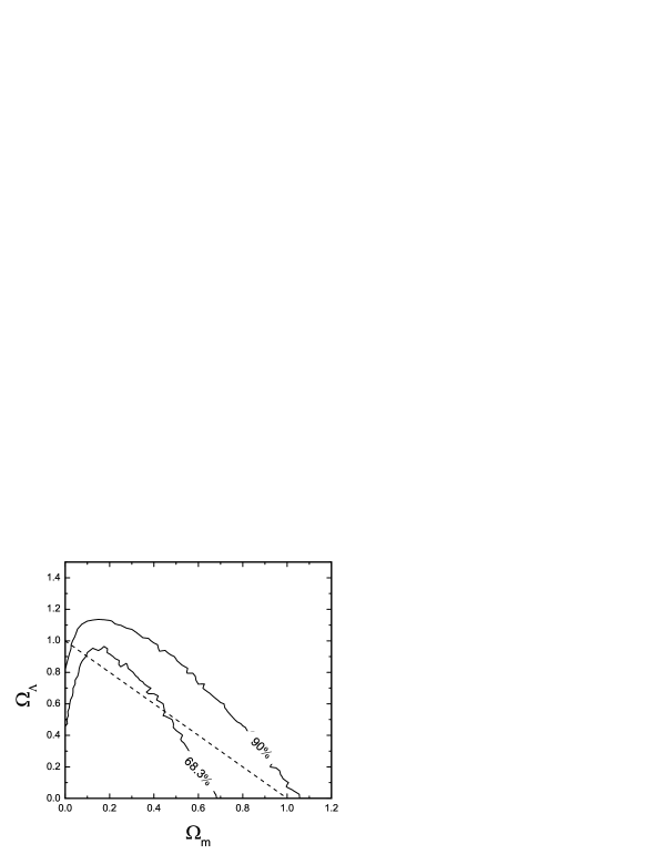
Figure 4: Contour confidence levels of $\Omega_{m}$ and $\Omega_{\Lambda}$, obtained by fitting the correlation with Method I.

Method II. The distance modulus of a GRB is defined as

$$\mu\equiv 5\log(D_{L}/10pc)\;,$$ (9)

in terms of the luminosity distance $D_{L}$. Using the Liang-Zhang relation, we can recast this in the form

$$\hat{\mu}=2.5[\kappa_{0}+\kappa_{1}\log E^{\prime}_{\rm p}+\kappa_{2}\log t^{\prime}_{\rm b}-\log(4\pi S_{\gamma}K)+\log(1+z)]-97.45\;.$$ (10)

However, since the luminosity correlation is cosmology-dependent, $\hat{\mu}$ also depends on the adopted expansion scenario. We use the following approach to circumvent this difficulty (see also Liang & Zhang 2005). This procedure is based on the calculation of the probability function for a given set of cosmological parameters (denoted by $\bar{\Omega}$, which includes both $\Omega_{m}$ and $\Omega_{\Lambda}$):

Step 1. For a given cosmological model, we calibrate and weight the luminosity indicator corresponding to each choice of parameters $\bar{\Omega}$. In each case, we calculate the correlation $\hat{E}_{\gamma,{\rm iso}}(\bar{\Omega};E^{\prime}_{\rm p},t^{\prime}_{\rm b})$, and evaluate the probability [$w(\bar{\Omega})$] of this relation being the optimal cosmology-independent luminosity indicator via $\chi^{2}$ statistics, i.e.,

$$\chi_{w}^{2}(\bar{\Omega})=\sum_{i}^{N}\frac{[\log\hat{E}_{\gamma,{\rm iso}}^{i}(\bar{\Omega})-\log E_{\gamma,{\rm iso}}^{i}(\bar{\Omega})]^{2}}{\sigma_{\log\hat{E}_{\gamma,{\rm iso}}^{i}}^{2}(\bar{\Omega})}\;.$$ (11)

The probability is then

$$w(\bar{\Omega})\propto e^{-\chi_{w}^{2}(\bar{\Omega})/2}\;.$$ (12)

Step 2. We regard the correlation derived for each set of parameters as a cosmology-independent luminosity indicator without considering its systematic error, and calculate the distance modulus $\hat{\mu}(\bar{\Omega})$ and its error $\sigma_{\hat{\mu}}$, given by

$$\sigma_{\hat{\mu}_{i}}=\frac{2.5}{\ln 10}\left[\left(\kappa_{1}\frac{\sigma_{E^{\prime}_{{\rm p},i}}}{E^{\prime}_{{\rm p},i}}\right)^{2}+\left(\kappa_{2}\frac{\sigma_{t^{\prime}_{{\rm b},i}}}{t^{\prime}_{{\rm b},i}}\right)^{2}+\left(\frac{\sigma_{S_{\gamma,i}}}{S_{\gamma,i}}\right)^{2}+\left(\frac{\sigma_{K_{i}}}{K_{i}}\right)^{2}+\left(\frac{\sigma_{z_{i}}}{1+z_{i}}\right)^{2}\right]^{1/2}.$$ (13)

Since both $(\sigma_{K_{i}}/K_{i})^{2}$ and $[\sigma_{z_{i}}/(1+z_{i})]^{2}$ are significantly smaller than the other terms in Equation (13), we ignore them in our calculations.

Step 3. We calculate the theoretical distance modulus $\mu(\Omega)$ for a set of cosmological parameters (denoted by $\Omega$), and then obtain $\chi^{2}$ from a comparison of $\mu(\Omega)$ with $\hat{\mu}(\Omega)$, i.e.,

$$\chi^{2}(\bar{\Omega}\mid\Omega)=\sum_{i}^{N}\frac{[\hat{\mu}_{i}(\bar{\Omega})-\mu_{i}(\Omega)]^{2}}{\sigma_{\hat{\mu}_{i}}^{2}(\bar{\Omega})}\;.$$ (14)

Step 4. We then calculate the probability that the cosmological parameter set $\Omega$ is the correct one according to the luminosity indicator derived from the cosmological parameter set $\bar{\Omega}$, i.e., we calculate

$$p(\bar{\Omega}\mid\Omega)\propto e^{-\chi^{2}(\bar{\Omega}\mid\Omega)/2}\;.$$ (15)

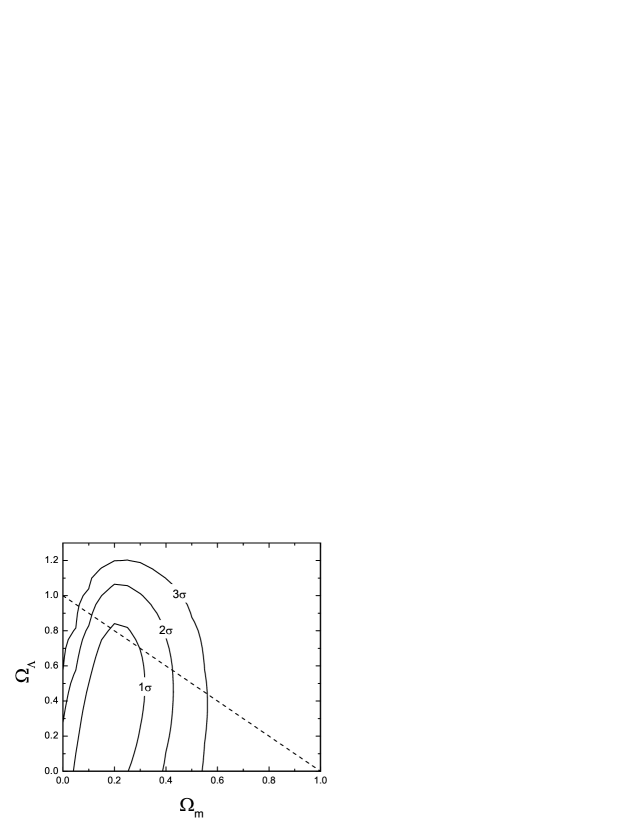
Figure 5: Contour confidence levels of $\Omega_{m}$ and $\Omega_{\Lambda}$, inferred from the current GRB sample, using method II.

Step 5. Finally, we integrate $\bar{\Omega}$ over the full cosmological parameter space to get the final normalized probability that the cosmological parameter set $\Omega$ is the correct one, i.e.,

$$p(\Omega)=\frac{\int_{\bar{\Omega}}w(\bar{\Omega})p(\bar{\Omega}\mid\Omega)\;d\bar{\Omega}}{\int_{\bar{\Omega}}w(\bar{\Omega})\;d\bar{\Omega}}\;.$$ (16)

Figure 5 shows the $1\sigma$ to $3\sigma$ contours of the probability in the ($\Omega_{m}$, $\Omega_{\Lambda}$) plane. The contours show that at the $1\sigma$ level, $0.04<\Omega_{m}<0.32$, but $\Omega_{\Lambda}$ is poorly constrained; only an upper limit of $\sim 0.84$ can be set at this confidence level. However, if we consider only a flat Universe, then the allowed range of parameter space is limited by the flat Universe dashed line and the $1\sigma$ contour, for which $0.19<\Omega_{m}<0.30$ and $0.7<\Omega_{\Lambda}<0.81$. The best fit values are $(\Omega_{m},\Omega_{\Lambda})=(0.25_{-0.06}^{+0.05},0.75_{-0.05}^{+0.06})$.

4 The $R_{\rm h}=ct$ Universe

In the previous section, we considered how the currently available sample of GRB events with spectral and lightcurve characteristics appropriate for cosmological work may be used to constrain the principal parameters of the standard model. The $R_{\rm h}=ct$ Universe, on the other hand, has only one free parameter—the Hubble constant $H_{0}$. However, as we have already noted, none of the results presented in this paper depend on this constant, since $1/H_{0}$ enters into the determination of both the data and the theoretical curves. There is therefore no need to reproduce the kind of parameter optimization for $R_{\rm h}=ct$ that was carried out for $\Lambda$CDM in § 3. But before we proceed to compare the Hubble diagrams for the $R_{\rm h}=ct$ Universe and the optimized $\Lambda$CDM model, we will first briefly summarize the $R_{\rm h}=ct$ cosmology, which is not yet as well known as $\Lambda$CDM.

One may look at the expansion of the Universe in several ways. From the perspective of the standard model, one guesses the constituents and their equation of state and then solves the dynamical equations to determine the expansion rate as a function of time. The second is to use symmetry arguments and our knowledge of the properties of a gravitational horizon in general relativity (GR) to determine the spacetime curvature, and thereby the expansion rate, strictly from just the value of the total energy density $\rho$ and the implied geometry, without necessarily having to worry about the specifics of the constituents that make up the density itself. This is the approach adopted by $R_{\rm h}=ct$. In other words, what matters is $\rho$ and the overall equation of state $p=w\rho$, in terms of the total pressure $p$ and total energy density $\rho$. In $\Lambda$CDM, one assumes $\rho=\rho_{m}+\rho_{r}+\rho_{de}$, i.e., that the principal constituents are matter, radiation, and an unknown dark energy, and then infers $w$ from the equations of state assigned to each of these constituents. In $R_{\rm h}=ct$, it is the aforementioned symmetries and other constraints from GR that uniquely fix $w$.

Both $\Lambda$CDM and $R_{\rm h}=ct$ are Friedmann-Robertson-Walker (FRW) cosmologies, but in the latter, Weyl’s postulate takes on a more important role than has been considered before (Melia & Shevchuk 2012). There is no modification to GR, and the Cosmological principle is adopted from the start, just like any other FRW cosmology. However, Weyl’s postulate adds a very important ingredient. Most workers assume that Weyl’s postulate is already incorporated into all FRW metrics, but actually it is only partially incorporated. Simply stated, Weyl’s postulate says that any proper distance $R(t)$ must be the product of a universal expansion factor $a(t)$ and an unchanging co-moving radius $r$, such that $R(t)=a(t)r$. The conventional way of writing an FRW metric adopts this coordinate definition, along with the cosmic time $t$. But what is often overlooked is the fact that the gravitational radius, $R_{\rm h}$ (see Equation 4), which has the same definition as the Schwarzschild radius, and actually coincides with the better known Hubble radius, is in fact itself a proper distance too (see also Melia & Abdelqader 2009). And when one forces this radius to comply with Weyl’s postulate, there is only one possible choice for $a(t)$, i.e., $a(t)=(t/t_{0})$, where $t_{0}$ is the current age of the Universe. This also leads to the result that the gravitational radius must be receding from us at speed $c$, which is in fact how the Hubble radius was defined in the first place, even before it was recognized as another manifestation of the gravitational horizon.

The principal difference between $\Lambda$CDM and $R_{\rm h}=ct$ is how they handle $\rho$ and $p$. In the $R_{\rm h}=ct$ cosmology, the fact that $a(t)\propto t$ requires that the total pressure $p$ be given as $p=-\rho/3$. The consequence of this is that quantities such as the luminosity distance and the redshift dependence of the Hubble constant $H$, take on very simple, analytical forms (as we have already seen in Equation 4). Though we won’t need it here, we also mention that the evolution of $H(z)$ in the $R_{\rm h}=ct$ Universe goes as

$$H(z)=H_{0}(1+z)\;,$$ (17)

another very simple and elegant expression that is not available in $\Lambda$CDM. Here, $z$ is the redshift, $R_{h}=c/H$, and $H_{0}$ is the value of the Hubble constant today. These relations are clearly very relevant to a proper examination of other cosmological observations, and we are in the process of applying them accordingly. For example, we have recently demonstrated that the model-independent cosmic chronometer data (see, e.g., Moresco et al. 2012) are a better match to $R_{\rm h}=ct$ (using Eq. 17), than the concordance, best-fit $\Lambda$CDM model (Melia & Maier 2013).

In the end, regardless of how $\Lambda$CDM or $R_{\rm h}=ct$ handle $\rho$ and $p$, they must both account for the same cosmological data. There is growing evidence that, with its empirical approach, $\Lambda$CDM can function as a reasonable approximation to $R_{\rm h}=ct$ in some restricted redshift ranges, but apparently does poorly in others. For example, in using the ansatz $\rho=\rho_{m}+\rho_{r}+\rho_{de}$ to fit the data, one finds that the $\Lambda$CDM parameters must have quite specific values, such as $\Omega_{m}\equiv\rho_{m}/\rho_{c}=0.27$ and $w_{de}=-1$, where $\rho_{c}$ is the critical density and $w_{de}$ is the equation-of-state parameter for dark energy. This is quite telling because with these parameters, $\Lambda$CDM then requires $R_{\rm h}(t_{0})=ct_{0}$ today. That is, the best-fit $\Lambda$CDM parameters describe a universal expansion equal to what it would have been with $R_{\rm h}=ct$ all along. Other indicators support the view that using $\Lambda$CDM to fit the data therefore produces a cosmology almost (but not entirely) identical to $R_{\rm h}=ct$ (see Melia 2012c).

As we shall see below, the results of our analysis of the GRB HD produce very similar conclusions to these, i.e., that even though the internal structure of $\Lambda$CDM would appear to be quite different from that in $R_{\rm h}=ct$ (compare Equations 2 and 4), in the end, the best fit $\Lambda$CDM model essentially mimics the universal expansion implied by $R_{\rm h}=ct$.

5 The GRB Hubble Diagram

In $\Lambda$CDM, the luminosity indicator, and therefore also the distance modulus $\mu$, depends on the specific choice of parameter values (for $\Omega_{m}$ and $\Omega_{\Lambda}$). To directly compare the HD for $\Lambda$CDM with that for $R_{\rm h}=ct$, we will calculate $\mu$ and $\sigma_{\mu}$ using the best-fit model, for which $\Omega_{m}=0.25$ and $\Omega_{\Lambda}=0.75$. The data and best-fit curve are shown together in the left-hand panel of Figure 6. The $\chi^{2}$ for this fit is calculated according to

$$\chi^{2}=\sum_{i}^{N}\frac{(\mu_{i}^{\rm obs}-\mu_{i}^{\rm th})^{2}}{\sigma_{\rm int}^{2}+\sigma_{\mu_{i}}^{2}}\;,$$ (18)

where $\mu^{\rm th}$ is theoretical value of the distance modulus, and $\mu^{\rm obs}$ is measured using the Liang-Zhang relation. Also, $\sigma_{\rm int}$ is the intrinsic scatter obtained from the joint likelihood analysis, and $\sigma_{\mu}$ is the error for each realization $\mu^{\rm obs}$ of the N data points. Ignoring $H_{0}$, which does not affect any of these fits, the optimized $\Lambda$CDM model has two remaining (principal) parameters, $\Omega_{m}$ and $\Omega_{\Lambda}$, so with 33 data points, the reduced $\chi^{2}$ per degree of freedom is $\chi^{2}_{\rm dof}=70.07/31=2.26$.

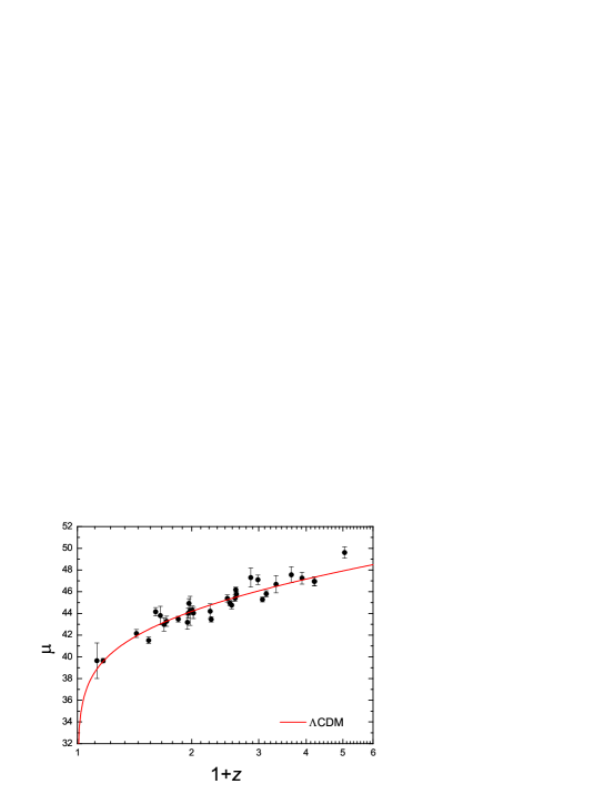
Figure 6: Left: Hubble diagram for the GRB sample. The solid curve represents the theoretical $\mu$ in the $\Lambda$CDM model. Right: Same as the left panel, except now the solid curve represents the $R_{h}=ct$ Universe.

The plot actually gives the impression that the fit is better than this $\chi^{2}_{\rm dof}$ would suggest. A closer inspection reveals that 5 data points lie more than $\sim 2\sigma$ away from the best-fit curve. Removal of these data reduces the $\chi^{2}$ considerably, and may be an indication that either they are true outliers, or that the errors and intrinsic scatter are greately underestimated.

The Hubble Diagram for the $R_{\rm h}=ct$ Universe is shown in the right-hand panel of Figure 6. Both the data and the best-fit curve were calibrated using the expansion implied by this cosmology (see column 5 in Table 2, and Equation 8). A Hubble constant $H_{0}=69.32$ km s^-1 Mpc^-1 was selected to construct the plot, though it has no bearing on the quality of the fit itself. In this case, since we are ignoring $H_{0}$ in producing the fit, there are no remaining free parameters, and the reduced $\chi^{2}$ per degree of freedom in $R_{\rm h}=ct$ is $\chi^{2}_{\rm dof}=70.53/33=2.14$. Strictly based on their $\chi^{2}_{\rm dof}$’s, the two fits are comparable, though some concern ought to be expressed about the possible contamination of the GRB sample by outliers and/or the underestimation of errors and intrinsic scatter. To facilitate a direct comparison, these two Hubble Diagrams are also shown side by side in Figure 7.

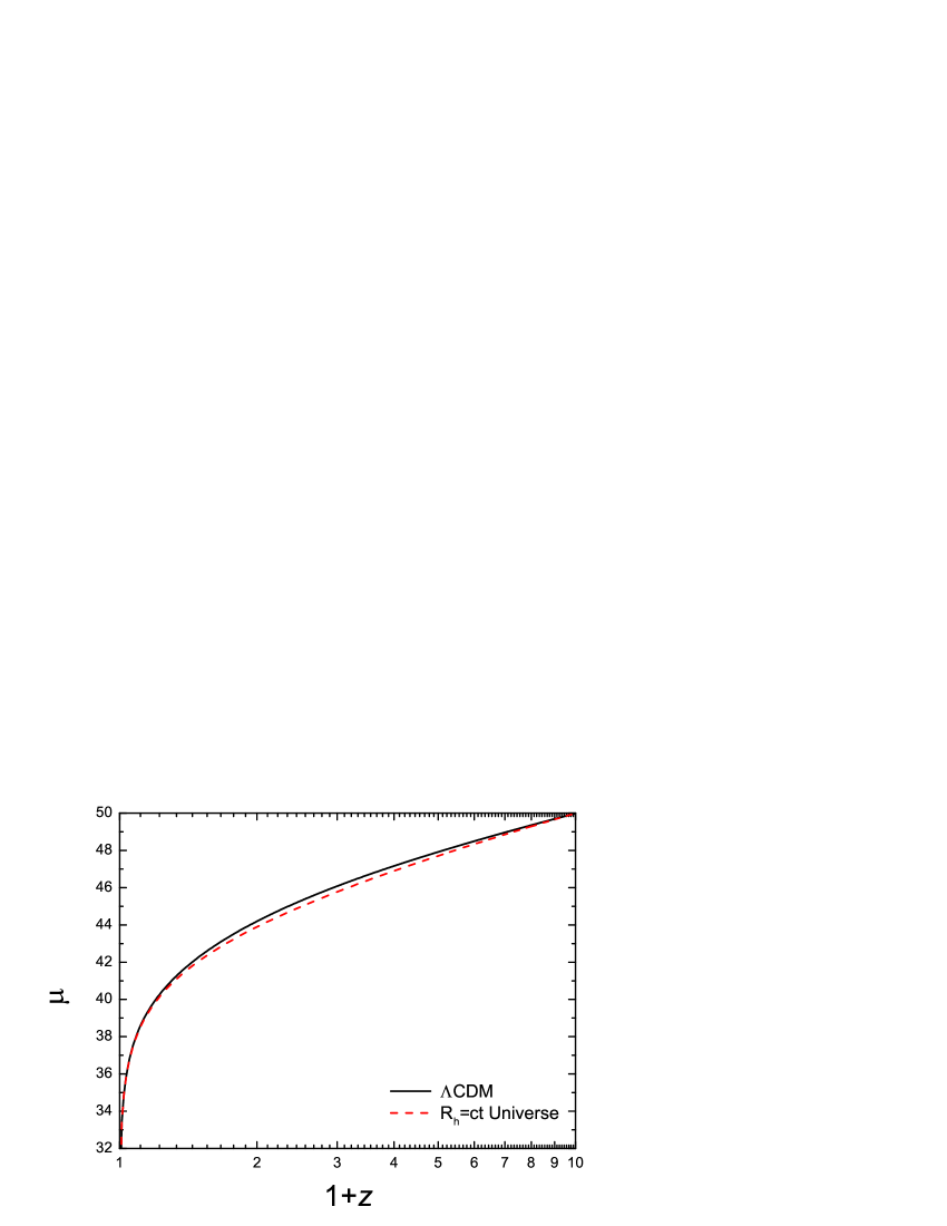
Figure 7: A side-by-side comparison of the theoretical curves in $\Lambda$CDM and the $R_{h}=ct$ Universe.

To determine the likelikhood of either $R_{\rm h}=ct$ or $\Lambda$CDM being closer to the “correct” model, we use the model selection criteria discussed extensively in Melia & Maier (2013). For such purposes, the Akaike Information Criterion (AIC) has become quite common in cosmology (see, e.g., Liddle 2004, 2007; Tan & Biswas 2012). The AIC prefers models with few parameters to those with many, unless the latter provide a substantially better fit to the data. This avoids the possibility that by using a greater number of parameters, one may simply be fitting the noise.

For each fitted model, the AIC is given by

$${\rm AIC}=\chi^{2}+2\,k\;,$$ (19)

where $k$ is the number of free parameters. If there are two models for the data, $\mathcal{M}_{1}$ and $\mathcal{M}_{2}$, and they have been separately fitted, the one with the least resulting AIC is assessed as the one more likely to be “true.” A more quantitative ranking of models can be computed as follows. If ${\rm AIC}_{\alpha}$ comes from model $\mathcal{M}_{\alpha}$, the unnormalized confidence that $\mathcal{M}_{\alpha}$ is true is the “Akaike weight” $\exp(-{\rm AIC}_{\alpha}/2)$. Informally, $\mathcal{M}_{\alpha}$ has likelihood

$${\cal L}(\mathcal{M}_{\alpha})=\frac{\exp(-{\rm AIC}_{\alpha}/2)}{\exp(-{\rm AIC}_{1}/2)+\exp(-{\rm AIC}_{2}/2)}$$ (20)

of being closer to the correct model. Thus, the difference ${\rm AIC}_{2}\nobreak-{\rm AIC}_{1}$ determines the extent to which $\mathcal{M}_{1}$ is favored over $\mathcal{M}_{2}$.

The choice of proportionality constant (i.e., $2$) for $k$ is not entirely arbitrary, being based on an argument from information theory that has close ties to statistical mechanics. (More details may be found in Melia & Maier 2013.) It is known that the AIC is increasingly accurate when the number of data points $N$ is large. However, in all cases, the magnitude of the difference $\Delta=\allowbreak{\rm AIC}_{2}-\nobreak{\rm AIC}_{1}$ provides a numerical assessment of the evidence that model 1 is to be preferred over model 2. A rule of thumb used in the literature is that if $\Delta\lesssim 2$, the evidence is weak; if $\Delta\approx 3$ or $4$, it is mildly strong; and if $\Delta\gtrsim 5$, it is quite strong.

Several alternatives to the AIC have been considered in the literature, but all are based on similar arguments. A lesser known one, called the Kullback Information Criterion (KIC), takes into account the fact that the PDF’s of the various competing models may not be symmetric. The unbiased estimator for the symmetrized version (Cavanaugh 1999) is given by

$${\rm KIC}=\chi^{2}+3\,k\;,$$ (21)

very similar to the AIC, but clearly strengthening the dependence on the number of free parameters (from $2k$ to $3k$). The rule of thumb concerning the strength of the evidence in KIC favoring one model over another is similar to that for AIC, and the likelihood is calculated using the same Equation (20), though with AIC_α replaced with KIC_α.

A better known alternative to the AIC is the Bayes Information Criterion (BIC), an asymptotic ($N\to\infty$) approximation to the outcome of a conventional Bayesian inference procedure for deciding between models (Schwarz 1978). This criterion is defined by

$${\rm BIC}=\chi^{2}+(\ln N)\,k,$$ (22)

and suppresses overfitting very strongly if $N$ is large. This criterion has already been used by Shi et al. (2012) to compare cosmological models. In this case, the evidence favoring one model over another is judged to be positive for a range of $\Delta\equiv{\rm BIC}_{1}-{\rm BIC}_{2}$ between 2 and 6, and is “strong” for values greater than this.

With the optimized fits we have obtained above, these three model selection criteria have the following values: for $R_{\rm h}=ct$, ${\rm AIC}_{1}=70.53$, ${\rm KIC}_{1}=70.53$, and ${\rm BIC}_{1}=70.53$. Whereas, for $\Lambda$CDM, we get ${\rm AIC}_{2}=74.07$, ${\rm KIC}_{2}=76.07$, and ${\rm BIC}_{2}=77.06$. Therefore, using the AIC, one finds that the likelihood of $R_{\rm h}=ct$ being closer to the correct cosmology is $85.4\%$, compared to only $14.6\%$ for $\Lambda$CDM. The difference is larger using the other criteria, which show that the $R_{\rm h}=ct$ Universe is favored over $\Lambda$CDM with a likelihood of $94.1\%$ versus $5.9\%$ using KIC, and $96.3\%$ versus $3.7\%$ using BIC. In showing the results of all three criteria, our principal goal is not so much to dwell on which of these may or may not reflect the importance of free parameters but, rather, to demonstrate a universally consistent outcome among the most commonly used model-selection tools in the literature. Clearly, the GRB Hubble Diagram favors $R_{\rm h}=ct$ over $\Lambda$CDM. Interestingly, these likelihoods are very similar to those inferred from our analysis of the cosmic chronometer data (Melia & Maier 2013), which showed that on the basis of those data, the $R_{\rm h}=ct$ Universe is favored over $\Lambda$CDM with a likelihood of $82-91\%$ versus $9-18\%$, for these three model selection criteria.

6 Discussion and Conclusions

In this paper, we have added some support to the argument that GRBs may eventually be used to carry out stringent tests on various cosmological models. Earlier work on this proposal had indicated that the spectral and lightcurve features most likely to provide a reliable luminosity indicator are the peak energy and a proxy for the jet opening angle, which we have taken to be the time at which a break in the light curve is observed. In this paper, we have confirmed the notion advanced previously that examining correlations among these data can indeed produce a luminosity indicator with sufficient reliability to study the expansion of the Universe.

A notable result of our work, based on the most up-to-date GRB data, is that a careful statistical analysis of these correlations and their optimization points to best-fit parameter values in $\Lambda$CDM remarkably close to those associated with the concordance model. We have found that the $\Lambda$CDM model most consistent with the GRB Hubble Diagram has $\Omega_{m}\approx 0.25$ and $\Omega_{\Lambda}\approx 0.75$. In the concordance model, these values are, respectively, $\approx 0.29$ and $\approx 0.71$ (Hinshaw et al. 2012).

However, for $\Lambda$CDM the reduced $\chi^{2}_{\rm dof}$ is at best approximately 2.26. A close inspection of the GRB HD for this model reveals that about $20\%$ of the data points lie at least $2\sigma$ away from the best-fit curve. This may be an indication that some contamination of the GRB sample is unavoidable, and that pure luminosity indicators may never be found for these sources. Of course, it could also mean that we simply have not yet found the ideal correlation function, and/or have not yet identified the correct spectral and lightcurve features to use for this purpose. On the other hand, it could also mean that we are understimating the errors and intrinsic scatter associated with the data. Additional work is required in order to better identify the likely resolution to this problem.

A second principal result of our analysis is that, based on fits to the GRB HD, the $R_{\rm h}=ct$ Universe is more likely to be closer to the “correct” model than the optimized $\Lambda$CDM. One of our goals with this work was to demonstrate the dependence of the data acquisition on the pre-assumed cosmological model. This appears to be an unavoidable problem with all cosmological data, except perhaps for the cosmic chronometer measurements which are obtained independently of any integrated quantity (such as the luminosity distance) that requires pre-knowledge of the Universe’s expansion history. By calibrating the GRB data separately for $\Lambda$CDM and $R_{\rm h}=ct$, we have produced a meaningful side-by-side comparison between these two cosmologies, showing that the latter fits the GRB HD with a reduced $\chi^{2}_{\rm dof}\approx 2.14$, compared to $2.26$ for the standard model. Nonetheless, these high values also show that the use of GRBs for cosmological purposes is not yet mature enough to carry out precision tests. However, in attempting to assess which of these two models is favored by the GRB data, we have found that several well-studied criteria developed for this purpose all consistently point to the $R_{\rm h}=ct$ Universe as being more likely to be correct than $\Lambda$CDM, with a likelihood of $\sim 85-96\%$ versus $\sim 4-15\%$.

Another significant result of our study is the remarkable overlap of the two best-fit curves in Figure 7. This feature is reminiscent of a similar result from our earlier study of Type Ia SNe, particularly Figure 4 in Melia (2012a). We believe that this is not a coincidence because several studies have now shown that $\Lambda$CDM is apparently mimicking the expansion history implied by $R_{\rm h}=ct$. The most detailed discussion on this issue has appeared in Melia (2012c; 2013). In these papers, we presented several arguments for why the optimization of the free parameters in $\Lambda$CDM always seems to indicate an overall expansion of the Universe equal to what it would have been in $R_{\rm h}=ct$.

Our final comment concerns the implications of this work on the use of Type Ia SNe to study the cosmological expansion at $z\lesssim 2$. There is no question now that any comparative analysis between competing cosmologies must be carried with the re-calibration of the data for each assumed expansion scenario, particularly when using standard candles that rely on integrated quantities, such as the luminosity distance. The Type Ia supernova luminosity cannot be determined independently of the assumed cosmology—it must be evaluated by optimizing 4 parameters simultaneously with those in the adopted model. This renders the data compliant to the underlying theory.

Given how much better $R_{\rm h}=ct$ accounts for the cosmological data, such as the angular correlation of the cosmic microwave background (Melia 2012d) and the redshift evolution of $H(z)$ (Melia 2013), not to mention the GRB HD we have studied in this paper, we believe it is necessary to produce a Type Ia supernova Hubble Diagram properly calibrated for the $R_{\rm h}=ct$ cosmology. Only then will it be possible to properly compare the best-fit $\Lambda$CDM model directly with $R_{\rm h}=ct$ at $z\lesssim 2$. The payoff from this effort should not be underestimated. We would know for certain whether the Universe is truly now accelerating, or whether it continues expanding at a constant rate, as it apparently has been doing from the beginning.

References

- Amati et al. (2002) Amati, L., Frontera, F., Tavani, M., et al. 2002, A&A, 390, 81
- Amati (2003) Amati, L. 2003, Chinese Journal of Astronomy and Astrophysics Supplement, 3, 455
- Amati (2006) Amati, L. 2006, MNRAS, 372, 233
- Amati et al. (2008) Amati, L., Guidorzi, C., Frontera, F., et al. 2008, MNRAS, 391, 577
- Ackermann et al. (2011) Ackermann, M., Ajello, M., Asano, K., et al. 2011, ApJ, 729, 114
- Andersen et al. (2003) Andersen, M. I., Masi, G., Jensen, B. L., & Hjorth, J. 2003, GRB Coordinates Network, 1993, 1
- Barth et al. (2003) Barth, A. J., Sari, R., Cohen, M. H., et al. 2003, ApJ, 584, L47
- Berger et al. (2002) Berger, E., Kulkarni, S. R., Bloom, J. S., et al. 2002, ApJ, 581, 981
- Berger et al. (2003) Berger, E., Kulkarni, S. R., Pooley, G., et al. 2003, Nature, 426, 154
- Bennett et al. (2012) Bennett, C. L., Larson, D., Weiland, J. L., et al. 2012, arXiv:1212.5225
- Björnsson et al. (2001) Björnsson, G., Hjorth, J., Jakobsson, P., Christensen, L., & Holland, S. 2001, ApJ, 552, L121
- Bloom et al. (2003) Bloom, J. S., Frail, D. A., & Kulkarni, S. R. 2003a, ApJ, 594, 674
- Bloom et al. (2003) Bloom, J. S., Morrell, N., & Mohanty, S. 2003b, GRB Coordinates Network, 2212, 1
- Blustin et al. (2006) Blustin, A. J., Band, D., Barthelmy, S., et al. 2006, ApJ, 637, 901
- Butler et al. (2010) Butler, N. R., Bloom, J. S., & Poznanski, D. 2010, ApJ, 711, 495
- (16) Cavanaugh, J. E. 1999, Statist. Probab. Lett., 42, 333
- Cenko et al. (2006) Cenko, S. B., Kasliwal, M., Harrison, F. A., et al. 2006, ApJ, 652, 490
- Cenko et al. (2011) Cenko, S. B., Frail, D. A., Harrison, F. A., et al. 2011, ApJ, 732, 29
- Chandra et al. (2008) Chandra, P., Cenko, S. B., Frail, D. A., et al. 2008, ApJ, 683, 924
- Collazzi et al. (2012) Collazzi, A. C., Schaefer, B. E., Goldstein, A., & Preece, R. D. 2012, ApJ, 747, 39
- Covino et al. (2008) Covino, S., D’Avanzo, P., Klotz, A., et al. 2008, MNRAS, 388, 347
- D’Agostini (2005) D’Agostini, G. 2005, arXiv:physics/0511182
- Dai et al. (2007) Dai, X., Halpern, J. P., Morgan, N. D., et al. 2007, ApJ, 658, 509
- Dai et al. (2004) Dai, Z. G., Liang, E. W., & Xu, D. 2004, ApJ, 612, L101
- Della Valle et al. (2006) Della Valle, M., Chincarini, G., Panagia, N., et al. 2006, Nature, 444, 1050
- Djorgovski et al. (1998) Djorgovski, S. G., Kulkarni, S. R., Bloom, J. S., et al. 1998, ApJ, 508, L17
- Djorgovski et al. (1999) Djorgovski, S. G., Goodrich, R., Kulkarni, S. R., et al. 1999, GRB Coordinates Network, 510, 1
- Djorgovski et al. (2001) Djorgovski, S. G., Frail, D. A., Kulkarni, S. R., et al. 2001, ApJ, 562, 654
- Firmani et al. (2005) Firmani, C., Ghisellini, G., Ghirlanda, G., & Avila-Reese, V. 2005, MNRAS, 360, L1
- Frail et al. (2001) Frail, D. A., Kulkarni, S. R., Sari, R., et al. 2001, ApJ, 562, L55
- Frail et al. (2003) Frail, D. A., Yost, S. A., Berger, E., et al. 2003, ApJ, 590, 992
- Fruchter et al. (1999) Fruchter, A. S., Thorsett, S. E., Metzger, M. R., et al. 1999, ApJ, 519, L13
- Galama et al. (2003) Galama, T. J., Reichart, D., Brown, T. M., et al. 2003, ApJ, 587, 135
- Garnavich et al. (1998) Garnavich, P. M., Jha, S., Challis, P., et al. 1998, ApJ, 509, 74
- Ghirlanda et al. (2004) Ghirlanda, G., Ghisellini, G., & Lazzati, D. 2004a, ApJ, 616, 331
- Ghirlanda et al. (2004) Ghirlanda, G., Ghisellini, G., Lazzati, D., & Firmani, C. 2004b, ApJ, 613, L13
- Ghirlanda et al. (2006) Ghirlanda, G., Ghisellini, G., Firmani, C., et al. 2006, A&A, 452, 839
- Ghirlanda et al. (2007) Ghirlanda, G., Nava, L., Ghisellini, G., & Firmani, C. 2007, A&A, 466, 127
- Ghirlanda et al. (2008) Ghirlanda, G., Nava, L., Ghisellini, G., Firmani, C., & Cabrera, J. I. 2008, MNRAS, 387, 319
- Ghirlanda (2009) Ghirlanda, G. 2009, American Institute of Physics Conference Series, 1111, 579
- Godet et al. (2005) Godet, O., Page, K. L., Goad, M. R., et al. 2005, GRB Coordinates Network, 3222, 1
- Golenetskii et al. (2007) Golenetskii, S., Aptekar, R., Mazets, E., et al. 2007, GRB Coordinates Network, 6879, 1
- Golenetskii et al. (2011) Golenetskii, S., Aptekar, R., Frederiks, D., et al. 2011, GRB Coordinates Network, 12008, 1
- Greiner et al. (2003) Greiner, J., Guenther, E., Klose, S., & Schwarz, R. 2003, GRB Coordinates Network, 1886, 1
- Guidorzi et al. (2011) Guidorzi, C., Lacapra, M., Frontera, F., et al. 2011, A&A, 526, A49
- Halpern et al. (2000) Halpern, J. P., Uglesich, R., Mirabal, N., et al. 2000, ApJ, 543, 697
- Hinshaw et al. (2012) Hinshaw, G., Larson, D., Komatsu, E., et al. 2012, arXiv:1212.5226
- Hjorth et al. (2003) Hjorth, J., Møller, P., Gorosabel, J., et al. 2003, ApJ, 597, 699
- Holland et al. (2002) Holland, S. T., Soszyński, I., Gladders, M. D., et al. 2002, AJ, 124, 639
- Holland et al. (2003) Holland, S. T., Weidinger, M., Fynbo, J. P. U., et al. 2003, AJ, 125, 2291
- Holland et al. (2004) Holland, S. T., Bersier, D., Bloom, J. S., et al. 2004, AJ, 128, 1955
- Jakobsson et al. (2003) Jakobsson, P., Hjorth, J., Fynbo, J. P. U., et al. 2003, A&A, 408, 941
- Jakobsson et al. (2004) Jakobsson, P., Hjorth, J., Fynbo, J. P. U., et al. 2004, A&A, 427, 785
- Jimenez et al. (2001) Jimenez, R., Band, D., & Piran, T. 2001, ApJ, 561, 171
- Kann et al. (2007) Kann, D. A., Laux, U., Filgas, R., et al. 2007, GRB Coordinates Network, 6935, 1
- Kann et al. (2011) Kann, D. A., Schmidl, S., Stecklum, B., & Hoegner, C. 2011, GRB Coordinates Network, 12010, 1
- Klose et al. (2004) Klose, S., Greiner, J., Rau, A., et al. 2004, AJ, 128, 1942
- Kocevski (2012) Kocevski, D. 2012, ApJ, 747, 146
- Kulkarni et al. (1999) Kulkarni, S. R., Djorgovski, S. G., Odewahn, S. C., et al. 1999, Nature, 398, 389
- Levinson & Eichler (1993) Levinson, A., & Eichler, D. 1993, ApJ, 418, 386
- Li et al. (2008) Li, H., Su, M., Fan, Z., Dai, Z., & Zhang, X. 2008, Physics Letters B, 658, 95
- Liang & Zhang (2005) Liang, E., & Zhang, B. 2005, ApJ, 633, 611
- Liang & Zhang (2006) Liang, E., & Zhang, B. 2006, MNRAS, 369, L37
- Liang et al. (2008) Liang, N., Xiao, W. K., Liu, Y., & Zhang, S. N. 2008, ApJ, 685, 354
- Liddle (2004) Liddle, A. R. 2004, MNRAS, 351, L49
- Liddle (2007) Liddle, A. R. 2007, MNRAS, 377, L74
- Lu et al. (2012) Lu, R.-J., Wei, J.-J., Liang, E.-W., et al. 2012, ApJ, 756, 112
- Möller et al. (2002) Möller, P., Fynbo, J. P. U., Hjorth, J., et al. 2002, A&A, 396, L21
- Martini et al. (2003) Martini, P., Garnavich, P., & Stanek, K. Z. 2003, GRB Coordinates Network, 1980, 1
- Melia (2007) Melia, F. 2007, MNRAS, 382, 1917
- Melia (2012) Melia, F. 2012a, AJ, 144, 110
- (72) Melia, F. 2012b, AJ, submitted
- (73) Melia, F. 2012c, MNRAS Letters, submitted
- Melia (2012) Melia, F. 2012d, AJ, submitted (arXiv:1207.0015)
- Melia (2013) Melia, F. 2013, ApJ, 764, 72
- Melia & Abdelqader (2009) Melia, F., & Abdelqader, M. 2009, IJMP-D, 18, 1889
- Melia & Maier (2013) Melia, F., & Maier, R. S. 2013, MNRAS, in press (arXiv:1304.1802)
- Melia & Shevchuk (2012) Melia, F., & Shevchuk, A. S. H. 2012, MNRAS, 419, 2579
- Molinari et al. (2007) Molinari, E., Vergani, S. D., Malesani, D., et al. 2007, A&A, 469, L13
- Moresco et al. (2012) Moresco, M., Verde, L., Pozzetti, L., Jimenez, R., & Cimatti, A. 2012, J. Cosmology Astropart. Phys, 7, 53
- Nicuesa Guelbenzu et al. (2011) Nicuesa Guelbenzu, A., Klose, S., Schmidl, S., et al. 2011, GRB Coordinates Network, 12239, 1
- Norris et al. (2000) Norris, J. P., Marani, G. F., & Bonnell, J. T. 2000, ApJ, 534, 248
- Perlmutter et al. (1998) Perlmutter, S., Aldering, G., della Valle, M., et al. 1998, Nature, 391, 51
- Perlmutter et al. (1999) Perlmutter, S., Aldering, G., Goldhaber, G., et al. 1999, ApJ, 517, 565
- Price et al. (2003) Price, P. A., Kulkarni, S. R., Berger, E., et al. 2003, ApJ, 589, 838
- Racusin et al. (2008) Racusin, J. L., Karpov, S. V., Sokolowski, M., et al. 2008, Nature, 455, 183
- Qi et al. (2008) Qi, S., Wang, F.-Y., & Lu, T. 2008a, A&A, 483, 49
- Qi et al. (2008) Qi, S., Wang, F.-Y., & Lu, T. 2008b, A&A, 487, 853
- Rhoads (1997) Rhoads, J. E. 1997, ApJ, 487, L1
- Riess et al. (1998) Riess, A. G., Filippenko, A. V., Challis, P., et al. 1998, AJ, 116, 1009
- Sagar et al. (2001) Sagar, R., Pandey, S. B., Mohan, V., Bhattacharya, D., & Castro-Tirado, A. J. 2001, Bulletin of the Astronomical Society of India, 29, 1
- Sakamoto et al. (2005) Sakamoto, T., Lamb, D. Q., Kawai, N., et al. 2005, ApJ, 629, 311
- Sakamoto et al. (2011) Sakamoto, T., Barthelmy, S. D., Baumgartner, W., et al. 2011, GRB Coordinates Network, 12276, 1
- Sari (1999) Sari, R. 1999, ApJ, 524, L43
- Schady et al. (2009) Schady, P., Baumgartner, W. H., & Beardmore, A. P. 2009, GCN Report, 232, 1
- Schaefer (2003) Schaefer, B. E. 2003a, ApJ, 583, L71
- Schaefer (2003) Schaefer, B. E. 2003b, ApJ, 583, L67
- Schaefer (2007) Schaefer, B. E. 2007, ApJ, 660, 16
- Schmidt et al. (1998) Schmidt, B. P., Suntzeff, N. B., Phillips, M. M., et al. 1998, ApJ, 507, 46
- (100) Schwarz, G. 1978, Ann. Statist., 6, 461
- Shi et al. (2012) Shi, K., Huang, Y. F., & Lu, T. 2012, MNRAS, 426, 2452
- Sholl et al. (2004) Sholl, M. J., Lampton, M. L., Aldering, G., et al. 2004, Proc. SPIE, 5487, 1473
- Stanek et al. (1999) Stanek, K. Z., Garnavich, P. M., Kaluzny, J., Pych, W., & Thompson, I. 1999, ApJ, 522, L39
- Stanek et al. (2005) Stanek, K. Z., Garnavich, P. M., Nutzman, P. A., et al. 2005, ApJ, 626, L5
- Su et al. (2006) Su, M., Li, H., Fan, Z., & Liu, B. 2006, arXiv:astro-ph/0611155
- Tan & Biswas (2012) Tan, M. Y. J., & Biswas, R. 2012, MNRAS, 419, 3292
- Tagliaferri et al. (2005) Tagliaferri, G., Antonelli, L. A., Chincarini, G., et al. 2005, A&A, 443, L1
- Vreeswijk et al. (2001) Vreeswijk, P. M., Fruchter, A., Kaper, L., et al. 2001, ApJ, 546, 672
- Vreeswijk et al. (2003) Vreeswijk, P., Fruchter, A., Hjorth, J., & Kouveliotou, C. 2003, GRB Coordinates Network, 1785, 1
- Wang & Dai (2006) Wang, F. Y., & Dai, Z. G. 2006, MNRAS, 368, 371
- Wang et al. (2011) Wang, F.-Y., Qi, S., & Dai, Z.-G. 2011, MNRAS, 415, 3423
- Wei & Gao (2003) Wei, D. M., & Gao, W. H. 2003, MNRAS, 345, 743
- Weidinger et al. (2003) Weidinger, M., Fynbo, J. P. U., Hjorth, J., et al. 2003, GRB Coordinates Network, 2215, 1
- Willott et al. (2010) Willott, C. J., Albert, L., Arzoumanian, D., et al. 2010, AJ, 140, 546
- Xiao & Schaefer (2009) Xiao, L., & Schaefer, B. E. 2009, ApJ, 707, 387
- Xu et al. (2005) Xu, D., Dai, Z. G., & Liang, E. W. 2005, ApJ, 633, 603
- Yonetoku et al. (2004) Yonetoku, D., Murakami, T., Nakamura, T., et al. 2004, ApJ, 609, 935