Effective Hamiltonian Crystal Field for Magnetic Interactions in Polynuclear Transition Metal Complexes. Sequential Derivation and Exemplary Numerical Estimates.

Abstract

By this we extend our work of the year 1992 devoted to calculating the intrashell excitations in the d-shells of coordination compounds of the first transition metal row, which resulted in the Effective Hamiltonian Crystal Field (EHCF) method, to their polynuclear analogs in order to assure the description of several open d-shells and of magnetic interactions of the effective spins residing in these shells. This is a challenging task since it requires improving the precision of ca. 1000 $\mathrm{cm}{}^{-1}$ (that of describing the excitation energies of the single d-shells by the already well successful EHCF method) to the that of ca. 10 $\div$ 100 $\mathrm{cm}{}^{-1}$ characteristic for the energies required to reorient the spins i.e. eventually by two orders of magnitude. This is performed within the same paradigm as used for the EHCF method: the concerted usage of the McWeeny’s group-function approximation and the Löwdin partition technique. These are applied to develop the effective description of the d-system of the polynuclear complexes, composed of several d-shells, including the working formulae for the exchange parameters between the d-shells belonging to different transition metal ions. These formulae are implemented in the package MagAîxTic and tested against a series of binuclear complexes of trivalent Cr and Fe cations featuring $\mu$-oxygen superexchange paths in order to confirm the reproducibility of the trends in the series of values of exchange parameters for the compounds differing by the chemical substitutions and other details of composition and structure. The results of calculations are in a reasonable agreement with available experimental data and other theoretical methods.

Moscow Center for Continuous Mathematical Education, Bol. Vlasevskiy per., 14, Moscow 119002, Russia

1 Introduction

Magnetic properties of transition metal complexes (TMC) derive from the classical work reducing them to those of the respective isolated d-shells.[1] Those of so called polynuclear TMC (PTMC - those containig two or more transition metal ions - TMI’s - with open d-shells) in the low-energy range are usually as well classically mapped to the effective exchange (spin) Dirac-Van Vleck-Heisenberg Hamiltonian:[2]

$$\hat{H}_{\mathrm{DvVH}}=\sum_{i<j}J_{ij}\hat{S}_{i}\hat{S}_{j},$$ (1)

controlled by the effective exchange parameters $J_{ij}$ describing the interactions of the effective spins $\hat{S}_{i}$ residing in the d-shells of the corresponding TMI’s with those in their neighbourhood. Numerous attempts have been undertaken to derive reliable numerical values of these parameters suitable to describe the lowest-energy range of excitations of the electronic subsystem of PTMCs quantum chemically. The complexity of this task (examples of the tentative application objects from the recent literature[3, 4, 5, 6] are quite impressive) prevented, however, from the decisive success. The theoretical considerations of the effective magnetic parameters present in the literature are numerous, but can be classified in three types: (i) ab initio approaches, (ii) DFT-based approaches, and (iii) semiempirical/semiquantitative approaches predominantly stemming from the solid state physics realm.

The ab initio methods are potentially capable to solve the problem (see below).[7, 8, 9, 10, 11] However, the systems of real interest in this area may contain thousands of atoms of which hundreds are going to be transition metal ones.[3, 4, 5, 6] Within the ab initio realm such systems require the account of correlations (both dynamical and noindynamical) at a level which causes the scaling of the requred computational resources as $N^{7}$ where $N$ is the number of orbitals involved. It will be hardly possible to apply such an approach within a chemical problem setting that of establishing/reproducing the trends in a series of similar compounds rather obtaining a unique number for a unique system. The dependence of the result on the basis state used has been established as well.[9]

The DFT based methods recently received considerable attention in this context. [12, 13] The success reported for the DFT-based techniques[12, 13] heavily relies upon the possibility to obtain the broken symmetry solutions in the UHF setting for the respective molecules. Although trivial for binuclear complexes, usual guinea pigs for the workers in the field, it may become very problematic for the systems where odd-numbered cycles of spins coupled through antiferromagnetic exchange interactions can be singled out and thus one can expect frustration, so that the spins cannot arrange themseves in a single strucutre describable by the Ising model which is a prerequisite for applying either the DFT-based technology or similar approach based on usage of nonempirical Hamiltonians. [12, 13]

These complications made us to reconsider the ingenious idea due to P.W. Anderson [16, 17] who suggested a two step procedure eventually yielding the reliable estimate of the magnetic exchange parameters without invoking a priori unknown magnetic ground states of a complex or a solid. According to the Anderson’s prescription (see also[18, 19]) in a line with the original implicit picture used by Bethe[1] formulated explicitly only later.[20] At the first step one has to obtain one-electronic wave functions of the magnetic ions (in our case these are the states of the TMI’s d-shells) immerced in the insulating diamagnetic medium (ligands) within some kind the ligand field theory.[21, 22] At the second step one has to estimate the interactions between electrons residing in the magnetic orbitals defined at the first step.

This way of thinking was pursued in our work[23] where we performed the first step: the consistent description of the magnetic states of the isolated TMIs. It is commonly believed that semi-empirical methods of quantum chemistry are not of much use for TMCs. The reason of such attitude originates from very narrow understanding of the nature of semiempirical methods. Of course, if one takes them naïvely: as a parameterized SCF in the valence basis, one cannot count on considerable success. Indeed, such an approach is known to be unsuccessful for decades in coping with the TMCs ground state total spins and with their geometry dependence not talking about the low-energy $d$-$d$ excitation spectra. The way out had been found[23] in the concerted usage of the McWeeny group-function formalism [24] and of the Löwdin partition technique[25] as described in details in reviews[26, 27] and in monograph.[28] This can be considered as a new concept of semiempirism in quantum chemistry: taking the form of the wave function on the basis of observable electronic groups (like d-shells, $\pi$-systems, two-center bonds etc.) characteristic for the considered class of molecules. Taking this way allowed us previously to reach considerable success in describing the ground states and $d$-$d$ excitation spectra of TMCs[23, 29, 30, 31, 32] and of their geometry dependence.[14, 15, 33, 34, 35, 36, 37, 38] In the present work we concentrate on the derivation of the effective Hamiltonian for the $d$-system of a PTMC which eventually contains necessary effective magnetic terms and by this follow the way (iii) of developing a substantiated semiempirical approach to estimating the parameters of effective magnetic interactions suitable for sizeable systems without addressing in advance their magnetic structure. This way would not be possible without works[39, 40, 41, 43, 42, 44, 45] where the quantitative empirical relations between the parameters of the crystal field felt by the d-shells in series of PTMCs and their respective magnetic exchange parameters has been firmly established. These phenomenological works allowed us to hope (and as shown below with good grounds) that the estimates of the crystal field parameters by semiempirical procedures assembled in the EHCF method[23] apply as well to the magnetic exchange parameters in PTMCs.

The paper is organized as follows. In the next Section we describe the necessary modification of the EHCF formalism for the case of polynuclear TMCs (PTMCs) and specific contributions to the effective Hamiltonian of their d-electrons. The details of the derivation are quite cumbersome and thus transferred to the Appendices. In further two Sections we describe respectively some relevant details of implementation and results of our calculations as compared to previous ones and the experiment. After that we discuss our results and the relation or our approach with others existing in this area.

2 Effective Hamiltonian of Crystal Field as modified for magnetic interactions

The intuitive physical picture we are going to pursue is very simple. The low-energy range of excitations of the electronic system of a polynuclear transition metal complex (PTMC) is spanned by the states differring by the relative orientations of the local spins (electronic in origin) residing in the respective d-shells. From the ab initio or DFT viewpoints such a picture is an enormous oversimplification since everyone is aware of the fact that all the basis electronic states are strongly hybridized. Nevertheless, the relative magnitudes of the electron transfer (hopping) matrix elements in comparison to the relevant energies of the one-electron charge transfer states differ drastically for different states within the PTMC. Namely, this ratio is by an order of magnitude larger for the transfers involving d-AOs than for a similar ratio for the transfers involving the AOs on the close ligand atoms. This is the physical reason why in most cases one can unequivocally ascribe some definite integer number of electrons to the d-shells and interpret the low-energy optical spectra of (P)TMCs in terms of the states of such shells with fixed integer numbers of electrons i.e. with use of the crystal field theory.[21, 22, 49] These ideas allowed us to make a formal move and to identify the parts of systems according to their respective different physical regimes: the highly correlated $d$-AOs which we term to span the one-electron space of the d-system and the weakly correlated AOs of the <<organogenic>> ligand atoms and the weakly correlated sp-AOs of TMI’s which span the one-electron space of the l-system. The difference of the physical conditions in so defined systems allows us treat them differently as well. The $l$-system being in a low correlated regime can be treated with an acceptable precision by a semiempirical SCF theory (INDO will suffice, see below); the d-system requires in principle kind of correlated treatment. In order to be able to treat so defined subsystems separately one has to develop (mutually dependent) effective Hamiltonians for the singled out subsystems. That for the d-system eventually contains the required <<magnetic>> terms. This development is sketched in the subsequent Subsections.

2.1 Molecular Hamiltonian breakdown

The basis of one-electron states for describing a PTMC is defined within a general semiempirical scheme and is thus spanned by the valence AOs which are considered to be implicitly orthogonal. For a PTMC the valence AO basis is formed by the valence AOs of the ligand atoms (largely, but not mandatory, organogenic) and by those of the TMIs it contains. These latter are the 4s-, 4p-, and 3d-AOs for the atoms of the first transition series. On the basis of the ratios of the characteristic intersubsystem hopping and Coulomb integrals we separate as explained previously the entire set of the AOs into the basis subsets spanning respectively d- and l-systems of a PTMC. The corresponding orbital subspaces are thus implicitly orthogonal.

According to the above classification of the valence AO’s the semiempirical Hamiltonian for a PTMC rewrites as (the explicit form of all operators is given in Appendix A):

$$\begin{array}[]{c}H=H_{d}+H_{l}+H_{\mathrm{int}}\\ H_{\mathrm{int}}=H_{c}+H_{r}+H_{x}\end{array}$$ (2)

where the operators $H_{d}$ (one for $d$-electrons of all TMIs in the complex) and $H_{l}$ (that for electrons in the l-system) are formally defined as those involving the Fermi creation and annihilation operators[46] referring only to the d- and l-systems, respectively, whereas the interaction operator $H_{\mathrm{int}}$ involves mixed products of the Fermi creation and annihilation operators referring to the d- and l-systems (see Appendix A.1).

The interaction operator $H_{\mathrm{int}}$ is a sum of contributions, which as well can be formally defined through the types of the products of the Fermi operators entering them. Correspondingly, the operators $H_{c}$ and $H_{x}$ are two-electron operators which involve the products of four Fermi operators and represent, respectively, the Coulomb and exchange interactions between two subsystems; the operator $H_{r}$ is the one-electron operator which involves only products of one Fermi operator referring to the d- and one Fermi operator referring to the l-AO subspaces (details see in Appendix A.2).

2.2 Configuration subspaces and Löwdin partitions

The main complication for a sequential description of magnetic properties of PTMCs is the enormous number of electronic configurations to be taken into account. Yet a simpler task of describing mononuclear TMCs involved quite a number of intermediate (<<outer space>>) configurations which were addressed with use of the Löwdin partition technique.[25] Its success as well as technical details of its implementation in the EHCF method makes us to try similar moves as applied to PTMCs. The Löwdin partition can be regarded as a specific method of separating variables in a many-particle system such that upon applying it, the system turns to be representable by a product function whose multipliers describe otherwise entangled states of the parts of the whole system. That is to say that performing a Löwdin partition is a prerequisite of employing the McWeeny group-function approximation. Thus our derivation evolves as a sequence of the Löwdin partitions allowing to single out relevant (<<model>>) configuration subspaces and to take into account the effect of the <<outer space>> configurations outside the model subspaces considered explicitly at each step on the matrix elements of the model Hamiptonian.

2.2.1 Separation of d- and l-electronic variables

The first move in the EHCF derivation was the separation of the variables in the single d-shell available in a mononuclear TMC and in the ligands. That finally allowed us to write the TMCs electronic wave function as an antisymmetrized product of the group functions for two distinguishable subsystems in the TMC, having physically different conditions, the d-shell and the rest:

$$\Psi_{\mathrm{TMC}}=\Phi_{d}\wedge\Phi_{L},$$ (3)

the form implicitly assumed by the crystal field theory.[1, 21, 22] The form eq. (3) is approximate since the operator $H_{r}$ acts and the electrons move between the subsystems so that the entire TMC occurs in an electronic state where those of the individual subsystems are entangled. In order to recover the crystal field theory picture in which the number of electrons in the d-system of the TMC is constant for the low-energy part of the electronic spectrum the exact Hamiltonian has to be projected to the model subspace spanned by the configurations in which the number of electrons in the $d$-shell(s) is fixed. The same move has to be done for the PTMCs. Let the overall number $n_{d}$ of electrons in the $d$-system be fixed. The numbers of electrons in the individual $d$-shells satisfy the following conditions:

$$\begin{array}[]{ccc}n_{l}&=&N-n_{d},\\ n_{d}&=&\sum_{i}n_{d}(i),\end{array}$$ (4)

where $n_{d}(i)$ is the number of electrons in the d-shell of the $i$-th TMI and $N$ is the total number of electrons in the PTMC. Since the states with different distributions of electrons among the $d$-shells of the different TMIs enter the consideration (see below) it may be technically easier to trace that $n_{l}$ – the number of electrons in the $l$-system – remains constant. As in the derivation of the EHCF method[23] the configurations with numbers of $d$- (or l-) electrons different from that fixed above (ligand to metal and metal to ligand charge transfer states, respectively abbreviated as LMCT and MLCT) have to be taken into account to keep track of the effect of the resonance operator $H_{r}$.

As in the derivation of the EHCF method[23] it is done with use the Löwdin partition technique.[25] Let $P$ be the projection operator to the model many-electron configuration subspace spanned by the Slater determinants with $n_{l}$ electrons in the l-system and remaining $n_{d}$ in all the $d$-shells and let $Q=1-P$ be its complementary projection operator. The Löwdin partition replaces the original Hamiltonian acting in the entire configuration space by the effective Hamiltonian $H^{\mathrm{eff}}(E)$ which acts in the model configuration subspace $\mathrm{Im}P$:

$$\begin{array}[]{c}H^{\mathrm{eff}}(E)=PHP+PH_{rr}P,\\ H_{rr}=H_{r}QR(E)QH_{r},\end{array}$$ (5)

but by construction has the same eigenvalues as the original Hamiltonian. In eq. (5) the resolvent:

$$R(E)\equiv(EQ-QHQ)^{-1}$$ (6)

is used. The form and the notation $H_{rr}$ is due to the fact that the operator $H_{r}$, the only term which transfers electrons between the $d$- and $l$-systems of the PTMC and by this mixes the states in the $\mathrm{Im}P$ and $\mathrm{Im}Q$ configuration subspaces,

$$\begin{array}[]{c}PHP=PH_{0}P+PH_{x}P\\ H_{0}=H_{d}+H_{l}+H_{c}\\ PHQ=PH_{r}Q;QHP=QH_{r}P\\ QHQ=QH_{0}Q+QH_{r}Q+QH_{x}Q\end{array}$$ (7)

ultimately enters the answer in an even degree. So we arrive to the effective Hamiltonian acting in the model configuration subspace with the fixed number of electrons in the d- and l-systems of a PTMC, but taking into account the LMCT and MLCT configurations in the <<outer>> configuration subspace.

The resolvent eq. (6) can be rewritten as a series with use of the bare resolvent:

$$R_{0}(E)\equiv(EQ-QH_{0}Q)^{-1}$$ (8)

derived from the operator $QH_{0}Q$ (conserving the quantities $n_{d}$ and $n_{l}$ which are thus <<good>> quantum numbers). The first terms in the series yield:

$$\begin{array}[]{c}R(E)=(EQ-QH_{0}Q-QH_{r}Q-QH_{x}Q)^{-1}\approx\\ \approx R_{0}(E)+R_{0}(E)\left(QH_{r}Q+QH_{x}Q\right)R_{0}(E)+\\ +R_{0}(E)\left(QH_{r}Q+QH_{x}Q\right)R_{0}(E)\left(QH_{r}Q+QH_{x}Q\right)R_{0}(E)\end{array}$$ (9)

When inserted in eq. (5) the above expression corresponds to the fourth order of perturbation theory with respect to the resonance operator $H_{r}$ and at least second order with respect to $H_{x}$. It is shown in Appendix B that the operator $H_{r}$ enters the effective Hamiltonian eq. (5) in a twofold way. First, the $H_{rr}^{(0)}$ component of $H_{rr}$ which results in no ionization of the l-system (formal definition of the compoments $H_{rr}^{(m\pm)}$ see Appendix B) acts within the model subspace $\mathrm{Im}P$ of our interest. Second, the $H_{rr}^{(2\pm)}$ components of $H_{rr}$ take into account the <<doubly ionic>> MLCT and LMCT configurations in which the l-system is doubly ionized in either sense. We denote these configurations as (LM)²CT or (ML)²CT with respect to the direction of the charge transfer. These configurations have been shown to be important for estimating the amount of effective antiferromagnetic interaction.[42] Collecting the relevant terms yields:

$$H^{\mathrm{eff}}(E) \approx PH_{0}P+PH_{x}P+PH_{rr}^{(0)}P+$$

$$+ PH_{r}^{(+)}Q^{(1+)}R_{0}^{(1+)}Q^{(1+)}H_{x}Q^{(1+)}R_{0}^{(1+)}Q^{(1+)}H_{r}^{(+)}P+$$

$$+ PH_{r}^{(-)}Q^{(1-)}R_{0}^{(1-)}Q^{(1-)}H_{x}Q^{(1-)}R_{0}^{(1-)}Q^{(1-)}H_{r}^{(-)}P+,$$

$$+ PH_{rr}^{(2+)}Q^{(2+)}R^{(2+)}Q^{(2+)}H_{rr}^{(2+)}P+$$

$$+ PH_{rr}^{(2-)}Q^{(2-)}R^{(2-)}Q^{(2-)}H_{rr}^{(2-)}P$$

which represents the approximate effective Hamiltonian acting in the subspace with the fixed distrubution of electrons between the d- and l-systems. For derivation of its individual terms see Appendix B.

2.2.2 Magnetic limit

In the previous Subsection we arrived to the effective Hamiltonian describing a PTMC in the configuration subspace with fixed distribution of electrons between the noncorrelated (diamagnetic) ligands and the correlated (potentially magnetic) d-shells of the TMIs. The purpose of this and subsequent Subsections is to derive the description of a PTMC in terms of its d-shells only. This is analogous to the description of a mononuclear TMC by its d-shell only, which is precisely the phenomenological crystal field theory[1, 21, 22] as sequentially derived in the frames of the EHCF approach.[23] Like there the variables referring to the l-system must be integrated out by taking an average over the approximate ground state $\left|\Phi_{L}\right\rangle$ of the $l$-system. The only formal requirement for the wave function $\left|\Phi_{L}\right\rangle$ is that it is a single determinant one:

$$\left|\Phi_{L}\right\rangle=\bigwedge\limits_{\lambda,\sigma}a_{\lambda\sigma}^{+}\left|0\right\rangle.$$ (11)

It can be thus either closed shell RHF, ROHF, or the UHF wave functions. The subscripts $\lambda,\sigma$ refer respectively for the l-MO and the spin projection.

The uncertainty in defining $\left|\Phi_{L}\right\rangle$ represents a problem. In the mononuclear TMC’s the definition of the configuration subspace in terms of the number of d-electrons $n_{d}$ was sufficient to define the effective electrostatic field induced by the TMI in the ligands, so that the ligands’ ground state $\left|\Phi_{L}\right\rangle$ could be calculated in this field with sufficient precision. In a PTMC the situation at this point is not that clear since electrons are allowed to travel between the d-shells of different TMI’s and such a redistribution produces too strong perturbation of the l-system to be accomodated by a single single-determinant wave function. For that reason we have to make an additional assumption, conforming, however, to our purpose of describing magnetic interactions. We assume that there exists a preferred distribution $\left\{n_{d}\left(i\right)\right\}$ of electrons among the TMI’s in the PTMC. Fixing this distribution defines the Coulomb field felt by the electrons in the ligands and thus $\left|\Phi_{L}\right\rangle$ can be calculated.

To formalize this move, which in fact reduces the description of the PTMC to the model configuration subspace where only the local electronic motions are allowed we define the projection operator acting in the subspace of the $n_{d}$-electronic states spanned by all possible determinants formed from AOs of the d-system with the fixed distribution of d-electrons:

$$\mathfrak{P}=\mathbb{O}\otimes I_{l},$$ (12)

where $I_{l}$ is the identity operator acting in the space of configurations of the l-system and $\mathbb{O}$ projects the configurations of the d-system on the subspace with the fixed numbers of electrons in each of the d-shells as formally defined by eq. (42) in Section C. The operator $\mathfrak{Q}$ is complementary to $\mathfrak{P}:$ $\mathfrak{P}+\mathfrak{Q}=\mathfrak{1}$.

With so defined projection operators we perform a further Löwdin partition as applied to the effective Hamiltonian $H^{\mathrm{eff}}(E)$ eq. (5) which results in another effective Hamiltonian:

$$\mathfrak{H}(E,\mathfrak{E})=\mathfrak{P}H^{\mathrm{eff}}\left(E\right)\mathfrak{P}+\mathfrak{P}H^{\mathrm{eff}}\left(E\right)\mathfrak{Q}\mathfrak{R}(\mathfrak{E})\mathfrak{Q}H^{\mathrm{eff}}\left(E\right)\mathfrak{P}$$ (13)

The resolvent is naturally of the form:

$$\mathfrak{R}(\mathfrak{E})=[\mathfrak{QE}-\mathfrak{Q}H^{\mathrm{eff}}\mathfrak{Q}]^{-1}$$ (14)

The action of the projection operators $\mathfrak{Q}$ and $\mathfrak{P}$ on the terms of the effective Hamiltonian $H^{\mathrm{eff}}(E)$ eq. (5) is:

$$\begin{array}[]{c}\mathfrak{P}PH_{0}P\mathfrak{P}+\mathfrak{P}PH_{x}P\mathfrak{P}\neq 0\\ \mathfrak{P}PH_{rr}P\mathfrak{P}\neq 0\\ \mathfrak{P}PH_{0}P\mathfrak{Q}=\mathfrak{Q}PH_{0}P\mathfrak{P}=0\\ \mathfrak{P}PH_{rr}P\mathfrak{Q}\neq 0;\mathfrak{Q}PH_{rr}P\mathfrak{P}\neq 0\\ \mathfrak{Q}H^{\mathrm{eff}}\mathfrak{Q}=\mathfrak{Q}P\left(H_{0}+H_{rr}+H_{x}\right)P\mathfrak{Q}\neq 0\end{array}$$ (15)

Only the nonvanishing term $\mathfrak{P}PH_{rr}P\mathfrak{Q}$ and its hermitean conjugate admix the states with charge transfer between the d-shells i.e. metal to metal charge transfer states (hereinafter abbreviated as MMCT) laying in the <<outer>> configuration space $\mathrm{Im}P\mathfrak{Q}$ to the states in our <<model>> space $\mathrm{Im}P\mathfrak{P}$.

2.2.3 Ligand integration and ligand polarization

Now we are almost ready to perform the final moves to eliminate the l-system variables. In variance with our original way[23] of reducing the effective Hamiltonian of the type of eqs. (5) and (13) acting in the restricted configuration space to one describing the mononuclear TMC in terms of its only d-shell which led us to the formal equivalent of the crystal field theory accompanied by the reliable estimates of the splitting parameters induced by this field[23] the situation in the PTMC’s is more complicated since it requires more complete dressing procedure for the d-electrons which eventually includes the effects of polarization of the ligand sphere (diamagnetic media in which the TMI’s are immerced) which accompany the virtual electron transfers from one d-shell to another. Such processes did not exist in the mononuclear case and for that reason had been originally neglected. It has been, however, explicitly shown that even in the mononuclear setting the polarization effects are responsible for the known nephelauxetic effect,[47, 48] which is the renormalization of the intrashell Coulomb (i.e. two-electronic) matrix elements due to indirect interaction between the fluctuations of the electronic density in the d-shell through the polarizations they induce in the ligands.[50] One may be sure that the partition described by eq. (5) does not lead to the description of the TMC by the wave function of the form eq. (3) rather by a description through a superposition of the functions of that form each corresponding to fixed number of electrons in the subsystems, but still entangled. In fact the operator $P$ projects out the states with the charge transfer between the $d$- and $l$-system, but does not assure the functional product form of eq. (3). Products of different states of the $d$- and $l$-systems satisfying only the condition of the fixed number of the electrons in each of the singled out groups enter in the expansion of the true ground state of the effective Hamiltonian eq. (5). The form eq. (3) is a kind of self consistent field approximation to it.[24] In order to improve this description one has to perform one more projection namely to the subspace of the products where all possible states of the $l$-system are replaced by its ground state. This is done as previously with use of the Löwdin projection using further projection operators. Let $\mathcal{P}$ be the projection operator on the ground state $\left|\Phi_{L}\right\rangle$ of the $l$-system:

$$\mathcal{P}=I_{d}\otimes\left|\Phi_{L}\right\rangle\left\langle\Phi_{L}\right|$$ (16)

complemented by the Kronecker product with $I_{d}$ - the identity operator with respect to the variables of the d-system. The complementary projection operator is $\mathcal{Q}=P\mathfrak{P}-\mathcal{P}$. Then applying the Löwdin partition as in the previous Subsections we arrive to the effective operator $\mathcal{H}^{eff}(E,\mathfrak{E},\Omega)$ which acts in the subspace of the configurations where the $l$-system is fixed in its ground state $\left|\Phi_{L}\right\rangle$:

$$\mathcal{H}^{\mathrm{eff}}(E,\mathfrak{E},\Omega)=\mathcal{P}\mathfrak{H(E)}\mathcal{P}+\mathcal{P}\mathfrak{H(E)}\mathcal{QR}(\Omega)\mathcal{Q}\mathfrak{H(E)}\mathcal{P}.$$ (17)

The Hamiltonian eq. (17) does not affect the variables in the l-system as described by its ground state $\left|\Phi_{L}\right\rangle$. Thus the effective Hamiltonian for the d-system can be easily obtained by dropping the bra- $\left\langle\Phi_{L}\right|$ on the right and the ket $\left|\Phi_{L}\right\rangle$ on the left in eq. (17) (namely in this order). Then the remaining averages over the wave function $\left|\Phi_{L}\right\rangle$ yield the sought effective Hamiltonian for the d-system only (the variables related to the l-system are integrated out). In the subsequent Sections we identfy in turn the individual contributions to it although the precise derivation of corresponding expressions will be kept in the respective Appendices. Further moves are stipulated by the projection to the single determinant ground state of the $l$-system as given by eq. (17). With use of the above generalized operators one can easily write the excited states relative to the single determinant ground state.

For completeness we calculate the resolvent part of the operator eq. (17). We notice that for the ground state of the vanishing total spin (closed shell) assumed hereinafter the following holds:

$$\mathcal{P}H_{x}\mathcal{P} = 0;$$

$$\mathcal{P}H_{x}\mathcal{Q} \neq 0$$

and calculate the second expression (or hermitean conjugate to it). It is also true that $\mathcal{P}H_{rr}^{(0)}\mathcal{Q}\neq 0$ and thus the operator $H_{rr}^{(0)}$ contributes to the second order according to

$$\begin{array}[]{c}\mathcal{P}H_{rr}^{(0)}\mathcal{R}(\Omega)H_{rr}^{(0)}\mathcal{P}=\\ \mathcal{P}H_{rr}^{(0)}(\mathcal{R}_{S}(\Omega)+\mathcal{R}_{T}(\Omega))H_{rr}^{(0)}\mathcal{P}=\\ \mathcal{P}H_{rr}^{(0)}\mathcal{R}_{S}(\Omega)H_{rr}^{(0)}\mathcal{P}+\mathcal{P}H_{rr}^{(0)}\mathcal{R}_{T}(\Omega)H_{rr}^{(0)}\mathcal{P}\end{array}$$

$\mathcal{R}_{S}(\Omega)$ and $\mathcal{R}_{T}(\Omega)$ contain respectively the projection operators to the singlet and triplet subspaces in the $\mathrm{Im}\mathcal{Q}$ subspace. The average $\left\langle\Phi_{L}\left|H_{rr}^{(0)}\mathcal{R}(\Omega)H_{rr}^{(0)}\right|\Phi_{L}\right\rangle$ contributes to the effective Hamiltonian for the $d$-electrons only.

3 Specific contributions to the d-system effective Hamiltonian.

As shown in the previous Section the contributions to the effective Hamiltonian for the d-system of a PTMC stem from averaging eq. (17) over $\left|\Phi_{L}\right\rangle$. As we mentioned in the previous Subsection the leading terms are those which appear from the first term of eq. (17) or equivalently the average of the entire Hamiltonian eq. (13). In the subsequent Subsections we consider them one by one.

3.1 Effective crystal field

The simplest contribution comes from the averaging the first term in eq. (13) directly contributing to the first term of eq. (17) over $\left|\Phi_{L}\right\rangle$.[23] The latter in its turn contains two contribution: the average of the Coulomb interaction over the ground state of the l-system $\left|\Phi_{L}\right\rangle$ which trivially (see Appendix D.1.3) yields the sum of the ionic/intraatomic contributions to the effective crystal field felt by the d-shells of the individual TMIs in a PTMC. It is consistently shown that the ionic contribution does not exceed 10% of the observed splitting.[15, 29, 30, 31, 32]

Nontrivial (and eventually the dominant) part of the latter is given by the average of the term $H_{rr}^{(0)}$ of the second order in $H_{r}$ originally performed while deriving the EHCF method for mononuclear TMCs.[23] Those derivation is generalized by treating individually the terms diagonal with respect to the TMI’s indices $ij$ as shown in Appendix D.1.4:

$$\begin{array}[]{c}\left\langle\Phi_{L}\right|\mathfrak{P}PH_{rr}^{(0)}P\mathfrak{P}\left|\Phi_{L}\right\rangle=\sum_{j}V_{\mathrm{CF}}^{\mathrm{cov}}(j)=\sum_{j}\sum\limits_{\mu\nu}\sum\limits_{\kappa\tau}\beta_{\mu\kappa}(j)\beta_{\nu\kappa}(j)\times\\ \left\{n_{\kappa}D^{(1+)}(j\kappa)d_{\nu\tau}^{+}(j)d_{\mu\tau}(j)-(1-n_{\kappa})D^{(1-)}(j\kappa)d_{\mu\tau}^{+}(j)d_{\nu\tau}(j)\right\}\end{array}$$ (18)

This operator due to projection operator $\mathfrak{P}$ represents precisely as denoted the sum of the covalent contributions to the effecitve crystal fields felt by the d-shells of the individual TMIs in the PTMC. Then the overall result of the averaging of $\mathfrak{P}H^{\mathrm{eff}}\mathfrak{P}$ reads:

$$\left\langle\Phi_{L}\left|\mathfrak{P}P\left(H_{0}+H_{rr}+H_{x}\right)P\mathfrak{P}\right|\Phi_{L}\right\rangle$$

$$= \sum_{i}\left\{H_{d}(i)+V_{\mathrm{CF}}^{\mathrm{ion}}(i)+V_{\mathrm{CF}}^{\mathrm{at}}(i)+V_{\mathrm{CF}}^{\mathrm{cov}}(i)\right.$$

$$\left.-2\sum_{\mu l}K_{\mu l}(i)\hat{S}_{\mu}(i)\left\langle\Phi_{L}\left|\hat{S}_{l}(i)\right|\Phi_{L}\right\rangle\right\}$$

The summation in the last term extends to the d-AOs $\mu$ and l-AOs l of the i-th TMI. It appears only if the spin density on the $l$-th AO of the $i$-th atom is nonvanishing. It is possible for the ROHF and UHF functions $\left|\Phi_{L}\right\rangle$ only and it is new as compared to the original EHCF[23] where only the RHF form of $\left|\Phi_{L}\right\rangle$ was allowed. However, hereinafter we concentrate on the systems in which in the zero approximation the ligands are diamagnetic, i.e. have no magnetic moments/spin densities in the l-system (and are thus representable by the RHF function) so that this term further is not going to reappear.

3.2 Magnetic contributions

In the previous Subsection we rederived the second order contribution of the one-electron hopping between the d- and l-systems to the effective Hamiltonian. Its part which is diagonal with respect to the TMI’s indices $i$ and j (or, equivalently, one acting within the configuration subspace $\mathrm{Im}\mathfrak{P}$) resulted as expected in the sum of the crystal field contributions for individual TMIs. The $ij$-off-diagonal part of $H_{rr}^{(0)}$ (that according to the formal expression $\mathfrak{P}H_{rr}^{(0)}\mathfrak{Q}$ coupling the configurations in the subspaces $\mathrm{Im}\mathfrak{P}$ and $\mathrm{Im}\mathfrak{Q}$) contributes to the effective operator for the d-system according to:

$$\begin{array}[]{c}\left\langle\Phi_{L}\left|\mathfrak{P}H_{rr}^{(0)}\mathfrak{Q}\mathfrak{R}(\mathfrak{E})\mathfrak{Q}H_{rr}^{(0)}\mathfrak{P}\right|\Phi_{L}\right\rangle=\\ \left\langle\Phi_{L}\left|\mathfrak{P}H_{rr}^{(0)}\mathfrak{Q}\left[\mathfrak{R}_{S}(\mathfrak{E})+\mathfrak{R}_{T}(\mathfrak{E})\right]\mathfrak{Q}H_{rr}^{(0)}\mathfrak{P}\right|\Phi_{L}\right\rangle\end{array}$$ (20)

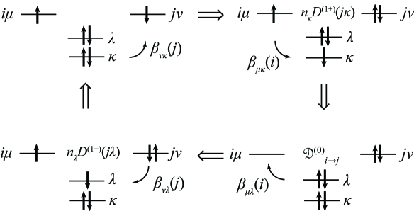
Figure 1: Sequence of configurations relevant to the matrix elements of type (a) as contributing to the effective exchange interaction in the case (i). The configuration in the upper left corner belongs to the model subspace $\mathrm{Im}P\mathfrak{P}$. The configurations in the upper right and lower left corners belong to the outer subspace $\mathrm{Im}Q^{(1+)}$ - that formed from the model space configurations by the LMCT states/processes, that in the lower right corner belongs to the outer subspace $\mathrm{Im}\mathfrak{Q}$ - that formed from the model space configurations by the MMCT states/processes. Transitions between the subspaces are indicated by the arrows, whereas the specific electron transfers by the arc arrows. The contributions to the exchange parameter are obtained as products of the quantities indicated in the Figure. The case (i) is characterized by the choice of the values of the energy denominators: namely those with the lowering spin in the both i-th and j-th d-shells.

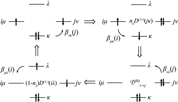
Figure 2: Sequence of configurations relevant to the matrix elements of type (b) as contributing to the effective exchange interaction in the case (i). The configurations in the upper right and lower left corners belong to the outer subspaces $\mathrm{Im}Q^{(1\pm)}$ - that formed from the model space configurations by the LMCT states/processes. Other notation is as in Fig. 1.

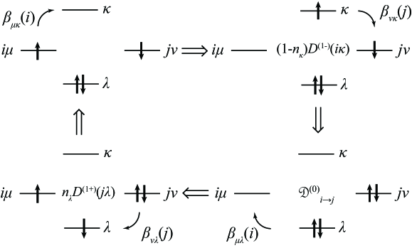
Figure 3: Sequence of configurations relevant to the matrix elements of type (c) as contributing to the effective exchange interaction in the case (i). The configurations in the upper right and lower left corners belong to the outer subspaces $\mathrm{Im}Q^{(1\mp)}$ - that formed from the model space configurations by the LMCT states/processes. Other notation is as in Fig. 1.

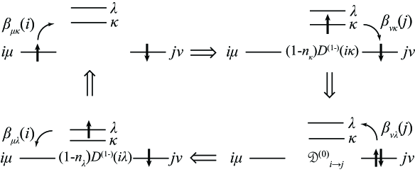
Figure 4: Sequence of configurations relevant to the matrix elements of type (d) as contributing to the effective exchange interaction in the case (i). The configurations in the upper right and lower left corners belong to the outer subspaces $\mathrm{Im}Q^{(1-)}$ - that formed from the model space configurations by the LMCT states/processes. Other notation is as in Fig. 1.

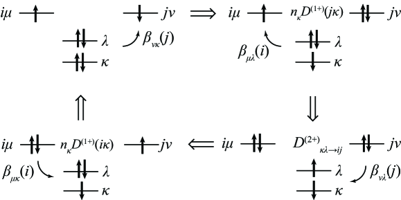
Figure 5: Sequence of configurations relevant to the matrix elements of type (e) as contributing to the effective exchange interaction in the case (i). The configurations in the upper right and lower left corners belong to the outer subspace $\mathrm{Im}Q^{(1+)}$ - that formed from the model space configurations by the LMCT states/processes, that in the lower right corner belongs to the outer subspace $\mathrm{Im}Q^{(2+)}$ - that formed from the model space configurations by the (LM)²CT states/processes. Other notation is as in Fig. 1.

by which the MMCT configurations are projected out. Formally it is nothing but the average of the second term in eq. (13). Eventually it represents the leading magnetic contribution. Details of the derivation are given in Appendix D.1. The corresponding configurations are shown in Figs. 1 - 4. They describe the situation which is conveniently described as effective one-electron transfers between different d-shells. However, it has been shown[42] that other processes having nothing to do with transfers of electrons between interacting d-shells rather those which can be described as correlated electron transfers between the l-system and the d-shells in which two electrons of the opposite spin projection are excited from a single l-MO to two d-shells under consideration. The correlations in this case is as well of <<kinematic>> nature and thus they contribute predominantly antiferromagnetically. The corresponding configurations are shown in Fig. 5. these contributions appear as a result of averaging the terms of the second order with respect to the ionizing components $H_{rr}^{(2\pm)}$ in eq. (40) of Appendix B.

The terms eqs. (56), (58) must be summed with the spin dependent factors assembled in Table D.2of Appendix D.2 and accroding to one of the four “cases” (i) - (iv) identified by Weihe and Güdel[40] to take into account the effect of the different variations of the spins in the d-shells involved in the electron transfer processes up on the contributions to the effective exchange between these d-shells. As one can see from Table D.2 the terms with different variation of the local spins contribute with different sign. The classification to the “cases” (i) - (iv) is based on the assumption that the transfer of an electron involving a half-filled orbital always result in a reduction of the local spins by $1/2$ in either of the involved d-shells irrespective to the sense of the transfer. If either of the involved orbitals is either completely occupied or empty the electron transfer process may result either in increase or decrease of the local spin by $1/2$ in the d-shell where such an orbital occurs. This results in only one contribution for the case (i), two contributions for the cases (ii) and (iii), and four contributions for the case (iv). These contributions enter with numerical unpairity factors specific for each case and with the signs specific for each combination of the possible variations of the local spins. The values of the energy denominators ($D^{(1\pm)},D^{(2\pm)},\mathfrak{D}^{(0)}$) referring to the intermediate states in the outer configuration subspaces must be taken according to the variation of the local spins specific for each contribution (that is to be higher by the intrashell exchange energy when the spin goes down and to be smaller by the same quantity when the spin goes up). That structure of the contributions and of their combinations entering the final expressions for the exchange parameters moved the authors[42] to expand the denominators’ products against the intraatomic exchange energies. Due to alternating signs of the contributions corresponding to the different conbinations of the intermediate local spins the terms of the lowest nonvanishing order survive for each of the cases (i) - (iv) which are respectively of the zeroth power for the case (i), of power one for the cases (ii) and (iii) and of the second power for the case (iv). This is how the expressions for the cases (i) - (iv) have been derived previously.[42] We do not use these expansions and employ “exact” values of the energy denominators.

Our derivation allows an additional classification according to the types of the terms in the sum over $\kappa\lambda$ which run through the l-MOs. These types (a) - (d) formally defined by eq. (57) correspond to the four possible transfer paths shown in Figs. 1 - 4 and respectively involving two occupied, two empty, and one empty and one occupied l-MOs in various orders. They describe contributions of the states in the MMCT configutation subspace and thus contain the energy denominator $\mathfrak{D}_{i\rightarrow j}^{(0)}$.

The values of these factors are generalized and summarized in Table 1. Each of these matrix elements contains the following expression:

$$\beta_{\nu\kappa}(j)\beta_{\mu\kappa}(i)\beta_{\mu\lambda}(i)\beta_{\nu\lambda}(j)\left[\mathfrak{D}_{i\rightarrow j}^{(0)}+n_{\kappa}n_{\lambda}D_{\kappa\lambda\rightarrow ij}^{(2+)}\right]$$ (21)

as a common factor. The first term in square brackets corresponds to an electron transfer from the i-th d-shell to the j-th one. The second term comes from the process of spin-correlated transfer of two electrons with opposite spin projections from the occupied l-MOs to the two d-shells by this effectuating coupling between them.

Table 1: Generalized factors of the matrix elements contributing to the exchange parameters.

a	$n_{\kappa}n_{\lambda}D^{(1+)}(j\lambda)D^{(1+)}(j\kappa)$
b	$-n_{\kappa}\left(1-n_{\lambda}\right)D^{(1+)}(j\kappa)D^{(1-)}(i\lambda)$
c	$-\left(1-n_{\kappa}\right)n_{\lambda}D^{(1-)}(i\kappa)D^{(1+)}(j\lambda)$
d	$\left(1-n_{\lambda}\right)\left(1-n_{\kappa}\right)D^{(1-)}(i\kappa)D^{(1-)}(i\lambda)$
e	$n_{\kappa}n_{\lambda}D^{(1+)}(j\lambda)\left[D^{(1+)}(i\kappa)+D^{(1+)}(j\lambda)\right]$
f	$\left(1-n_{\lambda}\right)\left(1-n_{\kappa}\right)D^{(1-)}(i\lambda)\left[D^{(1-)}(i\kappa)+D^{(1-)}(j\lambda)\right]$

In the previous Sections we were able to basically rederive and generalize the perturbative formulae for the contributions to the exchange in a form suitable for programming. They are also complemented by additional terms stemming from various processes involving polarization of the l-system. As expected the terms are numerous. However, additional considerations allow to range these terms in order of their importance. At the present first step we concentrate on the estimates of the contributions stemming from the electron transfers which are formally of the fourth power with respect to the one-electron hopping integrals $\beta$’s.

4 Details of implementation & calculation results

The formulae for the effective exchange parameters derived in the previous Sections do not require any additional quantities except those which are already calculated in the context of the EHCF method.[23] These are the l-MO LCAO expansion coefficients, respective orbital energies, d-AO-l-MO resonance integrals $\beta_{\mu\lambda}\left(i\right)$, etc. We implemented the derived formulae as a program suite accepting standard quantum chemical input (molecular composition and geometry) using the GEOMO package[51] (QCPE No 290) as a source of the subroutines for performing the calulations of the molecular integrals and performing semi-empirical SCF MO LCAO procedures for the l-system. The package has been tested agaist the compounds of the Cr(III)OCr(III) family[52, 53, 54, 55] known as <<basic rhodo>> compounds which have been synthetized by S.M. Jorgensen 130 years ago.[56] The parameterization procedure follows general EHCF methodology and will be described elsewhere.

We performed a series of calculations for those compounds studied in the phenomenological setting where the structural data were available. The results relative to the $\mu$-oxo bridged Cr(III) dimers are given in Table 2.

Table 2: Calculated and experimental values of the exchange parameters in $\mu$-oxo bridged Cr(III) dimers.

Compound (CCSD Code)	$J_{\mathrm{exp}}$, cm-1 Ref. [60]	$J_{\mathrm{calc}}$, cm-1	Geometry source
[(NH3)5CrOCr(NH3)5]4+	450	408	[52]
GAMTUJ	510	424	[53]
VIDTIL	100	190	[54]
ZUVMIM	60	150	[55]

As one can see the order of magnitude of the exchange parameters in this series of compounds is correctly reproduced as are their trends dependent on the chemical composition and bridge geometry (basic erhythro-compound [(NH₃)₅CrOCr(NH₃)₅]⁴⁺ and GAMTUJ have linear bridge geometry whereas VIDTIL and ZUVMIM are bent with the $\widehat{\mathrm{CrOCr}}$ angle in the range 128^∘$\div$132^∘) , although the amplitude of the angular dependence as obtained in the calculation is somewhat smaller than the experiemental one. Analogous calculations performed for the $\mu$-oxo bridged Fe(III) dimers (Table 3)

Table 3: Calculated and experimental values of the exchange parameters in $\mu$-oxo bridged Fe(III) dimers.

Compound (CCSD Code)	$J_{\mathrm{exp}}$, cm-1 Ref. [41]	$J_{\mathrm{calc}}$, cm-1	Geometry source
DIBXAN	238	240	[62]
VABMUG	264	256	[64]
PYCXFE	214	118	[61]
COCJIN deprotonated	242	110	[63]
COCJIN		30	[65]

show similarly reasonable agreement between the experimental and calculated values of the exchange constants.

The most remarkable feature we addressed in this context is the effect of protonation of the oxo-bridge upon the magnitude of the exchange constant. Comparing the calculated values in the last two lines of Table 3 we see that the protonation as expected breaks at least one of the superexchange paths going through the oxo-bridge which as expected as well significantly reduces the magnitude of the effective exchange parameter.

5 Conclusion

By this we extend our work [23] of the year 1992 devoted to calculating the intrashell excitations in the d-shells of coordination compounds of the first transition metal row, which resulted in the Effective Hamiltonian Crystal Field (EHCF) method, to their polinuclear analogs in order to assure the description of several open d-shells and of magnetic interactions of the effective spins residing in these shells. This is a challenging task since it requires improving the precision of ca. 1000 $\mathrm{cm}{}^{-1}$ (that of describing the excitation energies of the single d-shells by the already well successful EHCF method) to the that of ca. 10 $\div$ 100 $\mathrm{cm}{}^{-1}$ characteristic for the energies required to reorient the spins i.e. eventually by two orders of magnitude. This is performed within the same paradigm as used for the EHCF method: the concerted usage of the McWeeny’s group-function approximation and the Löwdin partition technique. These are used to develop the effective description of the d-system of the polynuclear complexes composed of several d-shells including the working formulae for the exchange parameters between the d-shells belonging to different transition metal ions. These formulae are implemented in the package MagAîxTic and tested against a series of binuclear complexes of trivalent cations featuring $\mu$-oxygen superexchange paths in order to confirm the reproducibility of the trends in the series of values of exchange parameters as well as the magnitude of these parameters for the compounds differing by the chemical substitutions and other details of composition and structure. The results of calculations are in a reasonable agreement with available experimental data and other theoretical methods.

Appendix A Hamiltonian contributions

A.1 Subsystem’s Hamiltonians

A.1.1 Hamiltonian for the d-System

The bare Hamiltonian for the d-system reads:

$$\sum_{i}H_{d}(i)+\frac{1}{2}\sum_{i\neq j}V_{\mathrm{Coul}}(ij)$$

The Hamiltonians for the individual d-shells are taken in the atomic symmetric approximation dating back to Refs. [66, 70, 69, 68, 67] so that the Coulomb interaction and the exchange splitting of d-electrons are decribed by two parameters ($U_{dd}(i)$ is the one-electron core-attraction parameter):

$$H_{d}(i)=U_{dd}(i)\hat{n}_{d}(i)+\frac{1}{2}g_{dd}(i)\hat{n}_{d}(i)\left(\hat{n}_{d}(i)-1\right)-K_{dd}(i)\hat{S}_{d}^{2}(i)$$ (22)

where $\hat{n}_{d}(i)$ is the operator of the number of particles, $\hat{S}_{d}(i)$ is the operator of the total spin, $U_{dd}(i)$ is the one-electron core attraction parameter, $g_{dd}(i)$ is the average parameter of the Coulomb interaction, $K_{dd}(i)$ is the average parameter of electronic exchange, all referring to the i-th d-shell. The main advantage of this form of the Hamiltonian is that it preserves a higher $SO(5)$ rather than the actual $SO(3)$ symmetry of the atom so that it remains invariant under arbitrary 5$\times$5 orthogonal transformation of the one-electron d-states. This will be necessary when going to the basis of the eigenstates of the local crystal field operator.

With such a bare Hamiltonian the state of the i-th d-shell is uniquely characterized by two quantum numbers: $n_{d}(i)$ - number of electrons, we use to build the configuration subspaces and to decompose the system in parts, and $S_{d}(i)$ - the total spin of the given $d$-shell. Then the energy of the entire manifold of the states with given $n_{d}(i)$ and $S_{d}(i)$ is given by:

$$U_{dd}(i)n_{d}(i)+\frac{1}{2}g_{dd}(i)n_{d}(i)\left(n_{d}(i)-1\right)-K_{dd}(i)S_{d}(i)\left(S_{d}(i)+1\right)$$ (23)

This form assures for the Hund’s rule for the states of the d-shells due to positiveness of the intrashell exchange parameters $K_{dd}(i)$ and for the compliance of the bare spectrum with the Landé interval’s rule as suggested in Refs. [48, 47]. The values of the core attraction parameters are taken as implemented in the EHCF package [23]. Those of the average interaction parameters are given by Jørgensen as well:

$$g_{dd}(i) = F_{dd}^{0}(i)-\frac{2}{63}\left(F_{dd}^{2}(i)+F_{dd}^{4}(i)\right)$$

$$K_{dd}(i) =\frac{35}{12} B(i)+\frac{7}{6}C(i)=\frac{5}{84}\left(F_{dd}^{2}(i)+F_{dd}^{4}(i)\right)$$

- not a very great improvement over Refs. [39, 40, 43, 42] where $B(i)$ and $C(i)$ are the Racah parameters for the i-th TMI and $F_{ll^{\prime}}^{k}\left(i\right)$ are the corresponding Slater-Condon parameters.

A.1.2 Hamiltonian for the l-system

INDO parameterization for the first row elements has been introduced in Ref. [72]. Its extensions to the transition metal atoms had been proposed in Refs. [73, 74, 75]. Within that setting the main problem was to implement intraatomic Coulomb and exchange two-electron integrals (Slater-Condon parameters $F^{k},G^{k}$) since wihtin the INDO (SCF) setting they cover all necessary intraatomic parameters allowed by symmetry. Rinaldi[51] have shown that the intraatomic configuration interaction involving s-, $p$-, and $d$-(sub)shells requires additional intraatomic integrals. These latter, however, again disappear if the d-shells enter the wave function as direct multipliers eq. (3). This is thus the case for the present method.

Then in the second quantization form the Hamiltonian for the $l$-system reads:

$$\begin{array}[]{c}H_{l}=\sum\limits_{m,\sigma}(U_{mm}-\sum\limits_{L}V_{ML})m_{\sigma}^{+}m_{\sigma}+\\ +\sum\limits_{L}\sum\limits_{l\in L,\sigma}(U_{ll}-\sum\limits_{L^{\prime}\neq L}V_{LL^{\prime}}-V_{LM})l_{\sigma}^{+}l_{\sigma}+\\ +\sum\limits_{ml,\sigma}\beta_{ml}(m_{\sigma}^{+}l_{\sigma}+h.c.)+\sum\limits_{ll^{\prime},\sigma}\beta_{ll^{\prime}}l_{\sigma}^{+}l_{\sigma}^{\prime}+\\ +\frac{1}{2}\sum_{ll^{\prime},\sigma}(ll^{\prime}\mid l^{\prime\prime}l^{\prime\prime\prime})l_{\sigma}^{+}l_{\tau}^{\prime\prime+}l_{\tau}^{\prime\prime\prime}l_{\sigma}^{\prime};\end{array}$$ (24)

here $l_{\sigma}^{+}$ ($l_{\sigma}$) are the creation (annihilation) of an electron with the spin projection $\sigma$ on an $l$-AO. First term in the expression eq. (24) describes the interaction of the $4s$- and $4p$-electrons of the metal ($m=4s,4p_{x},4p_{y},4p_{z}$) with the metal core (parameters $U_{mm}<0$) and the ligand atoms cores (parameters $V_{ML}>0$). Second term describes interaction of the ligand electrons with the ligand cores (parameters $U_{ll}<0$), with the cores of the other ligand atoms (parameters $V_{LL^{\prime}}>0$) and with the metal core (parameter $V_{LM}>0$). Third and fourth terms describe the resonance interactions in the ligand subsystem (parameters $\beta_{ml}<0$ and $\beta_{ll^{\prime}}<0$). Last term describes the Coulomb interactions between electrons ($(ll^{\prime}\mid l^{\prime\prime}l^{\prime\prime\prime})$ are the corresponding two-electron integrals).

A.1.3 Fockian for the l-system

The calculation of the wave function of the l-system is the prerequisite

Variation principle applied to the effective Hamiltonian with the trial function of the form eq. (3) leads to the self-consistent system of equations:

$$\begin{array}[]{ccl}H_{d}^{eff}\Phi_{n}^{d}&=&E_{n}^{d}\Phi_{n}^{d}\\ H_{l}^{eff}\Phi_{0}^{l}&=&E_{0}^{l}\Phi_{0}^{l}\\ H_{d}^{eff}&=&H_{d}+\left\langle\Phi_{0}^{l}\mid H_{c}+H_{rr}\mid\Phi_{0}^{l}\right\rangle,\\ H_{l}^{eff}&=&H_{l}+\left\langle\Phi_{0}^{d}\mid H_{c}+H_{rr}\mid\Phi_{0}^{d}\right\rangle.\end{array}$$ (25)

In the above system the effective Hamiltonian $H_{d}^{eff}$ for the $d$-electron subsystem depends on the wave function of the ligand subsystem $\Phi_{0}^{l}$, and in its turn the effective Hamiltonian $H_{l}^{eff}$ for the ligand susbsytem depends on the $d$-electrons’ wave functions $\Phi_{0}^{d}$. These equations must be solved self-consistently as well. In the EHCF method Ref. [23] the Slater determinant $\Phi_{0}^{l}$, is constructed of MO’s of the $l$-system, obtained from the Hartree-Fock equations in the INDO approximation for the valence electrons of the ligands. In this case the transition from the bare Hamiltonian $H_{l}^{eff}$ for the $l$-system to the corresponding effective (dressed) Hamiltonian reduces to renormalization of one-electron parameters related to the TMI:

$$\begin{array}[]{c}U_{ii}^{eff}=U_{ii}+\frac{1}{5}n_{d}\sum\limits_{\mu}g_{\mu i},\\ Z_{M}^{eff}=Z_{M}-n_{d},\end{array}$$ (26)

where $U_{ii}$ is the parameter of the interaction of $4s$ and $4p$-electrons ($i=4s$, $4p_{x}$, $4p_{y}$, $4p_{z}$) with the TMI core, $Z_{M}$ is TMI core charge, $g_{\mu i}=(\mu\mu|ii)-\frac{1}{2}(\mu i|i\mu)$ are the parameters of intraatomic Coulomb interactions. The $\Phi_{0}^{l}$ function thus obtained is used further for constructing the effective Hamiltonian for the $d$-shell.

A.2 Intersubsystem interaction operators

Here we introduce explicit definitions for the interaction operators acting between the d- and l-system of a PTMC.

A.2.1 dl-Resonance operator

The resonance operator $H_{r}$ describing one-electron hopping between the d-shells and the ligands has the form:

$$H_{r} = H_{r}^{(+)}+H_{r}^{(-)},$$

$$H_{r}^{(+)} = -\sum_{\sigma}\sum_{\mu,i}\sum_{\lambda}\beta_{\mu\lambda}(i)d_{\mu\sigma}^{+}(i)a_{\lambda\sigma},$$ (27)

$$H_{r}^{(-)} = -\sum_{\sigma}\sum_{\mu,i}\sum_{\lambda}\beta_{\mu\lambda}(i)a_{\lambda\sigma}^{+}d_{\mu\sigma}(i),$$

where $\lambda$ runs over $l$-MOs, $\beta_{\mu\lambda}(i)$ is the resonance (hopping) integral between the $\mu$-th $d$-AO of the $i$-th TMI and the $\lambda$-th $l$-MO, the fermion operator $d_{\mu\sigma}^{+}(i)$ creates an electron with the spin projection $\sigma$ on the $\mu$-th $d$-AO of the $i$-th TMI, and $a_{\lambda\sigma}^{+}$ creates an electron with the spin projection $\sigma$ on the $\lambda$-th $l$-MO. One can easily check that the terms $H_{r}^{(\pm)}$ are the hermitean conjugates of each other. Action of $H_{r}^{(+)}$apparently results in positive ionization of the l-system ($l\rightarrow d$ one-electron transfer), that of $H_{r}^{(-)}$ refers to the negative ionization of the l-system ($d\rightarrow l$ one-electron transfer). The above definition can be somewhat simplified by using the spinor notation:

$$H_{r}^{(+)} = -\sum_{\mu,i}\sum_{\lambda}\beta_{\mu\lambda}(i)d_{\mu}^{+}(i)\hat{\iota}a_{\lambda},$$ (28)

$$H_{r}^{(-)} = -\sum_{\mu,i}\sum_{\lambda}\beta_{\mu\lambda}(i)a_{\lambda}^{+}\hat{\iota}d_{\mu}(i).$$

A.2.2 dl-Coulomb and exchange operators

Although fundamentally we rely upon the INDO approximation for the bare Hamiltonian for the PTMC we have to make certain concessions and regrouping of terms in order to profit from the symmetries characteristic for the atomic problem. Specifically we separate the Coulomb interaction into symmetric (superscript “(s)”) and asymmetric (superscript “(a)”) parts of which the first incures only the uniform shift of the d-levels in each given TMI whereas the second induces the splitting of the otherwise degenerate d-levels. The symmetry mean by the symmetric part is that of the $SO(5)$ - i.e. of an arbitarary orthogonal transformation of the d-orbitals. These two contributions further subdivide into an interaatomic (marked by subscript <<1>>) part describing the interactions with the electrons in the noncorrelated sp-AOs of a given TMI and the interatomic one describing the interactions with electrons residing on other atoms (marked by subscript <<2>>). With these assumptions the Coulomb interaction between the subsystems of a PTMC reads:

$$H_{c} = H_{c}^{(s)}+H_{c}^{(a)}$$

$$H_{c1}^{(s)} = \sum_{i}\sum_{L}\hat{n}_{d}(i)\left[\hat{n}_{s}(i)F_{i}^{0}(sd)+\hat{n}_{p}(i)F_{i}^{0}(pd)\right]$$

$$H_{c2}^{(s)} = e^{2}\sum_{i}\sum_{L}\hat{n}_{d}(i)\hat{n}_{L}F_{0}(R_{Li})$$ (29)

$$H_{c1}^{(a)} = \sum_{i\mu}\sum_{L}\hat{n}_{\mu}(i)\hat{n}_{\gamma}(i)g_{\mu\gamma}^{pd}(i)$$

$$H_{c2}^{(a)} = \sum_{mm^{\prime}}\hat{V}_{mm^{\prime}};\hat{n}_{d}(i)=\sum_{\mu}\hat{n}_{\mu}(i)$$

where $\hat{n}_{d}(i)$ and $\hat{n}_{l}$ are the operators of the numbers of electrons in the $i$-th d-shell and on the $l$-th $l$-AO; $\hat{n}_{\mu}(i)$ is that for the $\mu$-th $d$-AO of the $i$-th TMI; $L$ stands for all orbitals $l$ centered on the ligand atom $L$; $\gamma=x,y,z$ $g_{\mu l}(i)$ are the energy parameters (in fact – the average Coulomb interaction integrals) and the interatomic contributions $\hat{V}_{mm^{\prime}}$ are given by:

$$\hat{V}_{mm^{\prime}} = \sum_{L}\sum_{\begin{subarray}{c}l\in L\\ \sigma,\tau\end{subarray}}V_{mm^{\prime}}^{L}d_{m\sigma}^{+}d_{m^{\prime}\sigma}l_{\tau}^{+}l_{\tau}$$

with

$$V_{mm^{\prime}}^{L}=5\sqrt{4\pi}\sum_{k=2,4}\frac{(-1)^{m}}{\sqrt{2k+1}}\left(\begin{array}[]{ccc}2&k&2\\ 0&0&0\end{array}\right)\left(\begin{array}[]{ccc}2&k&2\\ m&m^{\prime}-m&-m^{\prime}\end{array}\right)F_{k}(R_{L})Y_{k}^{m-m^{\prime}}(\theta_{L},\phi_{L}).$$ (30)

where $(R_{L},\theta_{L},\phi_{L})$ are the spherical coordinates of the ligand atom $L$ (relative to a TMI consequently located in the center of the coordinate frame); $Y_{k}^{m-m^{\prime}}(\theta_{L},\phi_{L})$ are the spherical functions with the phases defined following Condon and Shortley.[71] Functions $F_{k}(R_{L})$ are the integrals of squares of the radial parts $R_{nl}(r)$ of the atomic $d$-functions:

$$F_{k}(R)=R^{-(k+1)}\int\limits_{0}^{R}r^{k}R_{nl}^{2}(r)r^{2}dr+R^{k}\int\limits_{R}^{\infty}r^{-(k+1)}R_{nl}^{2}(r)r^{2}dr$$ (31)

depend on the distance $R_{L}$ from the atom of metal to the atom $L$. For the Slater AOs $R_{nl}(r)$ the functions $F_{k}(R)$ are explicitly known.[22]

Experience of usage of the EHCF numerical procedure acquired so far shows that the effect of the Coulomb splitting (asymmetric part of the Coulomb interaction) can be safely neglected when it goes about estimating the energy denominators in the resolvent in Section C.1 which is done consistently.

The exchange operator decomposes analogously with that difference that in the INDO approximation only the intraatomic contribution on the TMIs is present.

$$H_{x} = H_{x}^{(s)}+H_{x}^{(a)}$$ (32)

We however restrict ourselves by the symmetric part of the intraatomic intershell exchange for the time being:

$$H_{x}^{(s)} = -2\sum_{i}\sum_{\begin{subarray}{c}\mu\in d\text{-}\mathrm{AO}\\ l\in l\text{-}\mathrm{AO}\end{subarray}}\hat{S}_{d}(i)\left[K_{sd}(i)\hat{S}_{s}(i)+K_{pd}(i)\hat{S}_{p}(i)\right]$$ (33)

$$\hat{S}_{d}(i) = \sum_{\mu}\hat{S}_{\mu}(i)$$

where $\hat{S}_{\mu}(i)$ and $\hat{S}_{l}(i)$ are the electron spin operators for electrons in the $\mu$-th $d$-AO of the $i$-th TMI and the $l$-th $l$-AO of the $i$-th TMI. The exchange parameters are given by:

$$K_{sd}(i) = \frac{1}{5}G_{sd}^{2}(i)$$

$$K_{pd}(i) = \frac{2}{15}G_{pd}^{1}(i)+\frac{113}{1225}G_{pd}^{3}(i)$$ (34)

Appendix B Expansion of the resolvent eq. (6)

Inserting the expansion of the resolvent eq. (6) in eq. (5) we obtain:

$$H^{\mathrm{eff}}(E) = PH_{0}P+PH_{x}P+$$

$$+PH_{r}QR_{0}QH_{r}P+$$

$$+PH_{r}QR_{0}QH_{x}QR_{0}QH_{r}P+$$

$$+PH_{r}QR_{0}QH_{r}QR_{0}QH_{r}QR_{0}QH_{r}P+$$

$$+PH_{r}QR_{0}QH_{x}QR_{0}QH_{x}QR_{0}QH_{r}P+\ldots$$

In the above expression (and in its continuation whatsoever) the odd powers of $H_{r}$ disappear since the operator $H_{r}$ changes the number of electrons in the $d$- and l-systems by one in either sum, and in case when the number of such changes is odd the total number of electrons in the $d$- and/or l-systems cannot be conserved. Thus the number of the $H_{r}$ multipliers must be even.

Further analysis can be based on the notion of "graduality" of the complementary projection operator $Q$ and the resolvent expressed by the following expansion for these quantities:

$$\begin{array}[]{c}Q=\bigoplus\limits_{n}Q^{(n\pm)}\\ R_{0}=\bigoplus\limits_{n}R^{(n\pm)}\end{array}$$ (36)

where $n$ refers to the number of electrons added to (”$+$”) or taken from (”$-$”) the $d$-system (this notation precisely refers to the degree of ionization of the l-system), and $\oplus$ stands for the direct (block) sum of the corresponding matrices. For the terms in eq. (36) the following orthogonality conditions hold:

$$\begin{array}[]{c}Q^{(n\pm)}R^{(m\pm)}Q^{(p\pm)}=\delta_{nm}\delta_{mp}R^{(m\pm)}\\ Q^{(m\pm)}R^{(n\pm)}P=PR^{(n\pm)}Q^{(m\pm)}=0\end{array}$$

With this decomposition for the resolvent and graduation of the $\mathrm{Im}Q$ configuration subspace the effective Hamiltonian rewrites:

$$H^{\mathrm{eff}}(E) = P\left(H_{0}+H_{x}\right)P+$$

$$+ PH_{r}Q^{(1\pm)}R^{(1\pm)}Q^{(1\pm)}H_{r}P+$$

$$+ PH_{r}Q^{(1\pm)}R^{(1\pm)}Q^{(1\pm)}H_{x}Q^{(1\pm)}R^{(1\pm)}Q^{(1\pm)}H_{r}P+$$

$$+ PH_{r}Q^{(1\pm)}R^{(1\pm)}Q^{(1\pm)}H_{r}Q^{(2\pm)}R^{(2\pm)}Q^{(2\pm)}H_{r}Q^{(1\pm)}R^{(1\pm)}Q^{(1\pm)}H_{r}P+$$

$$+ PH_{r}QR_{0}QH_{x}QR_{0}QH_{x}QR_{0}QH_{r}P+...$$

where the terms with <<+>> and <<->> superscripts are summed separately.

As for the terms containing the powers of the exchange operator $H_{x}QR_{0}$ only they seem to be summable since they involve only the terms of the same graduality. It looks like:

$$PH_{r}QR_{0}QH_{x}QR_{0}QH_{r}P+$$

$$PH_{r}QR_{0}QH_{x}QR_{0}QH_{x}QR_{0}QH_{r}P+$$

$$PH_{r}QR_{0}QH_{x}QR_{0}QH_{x}QR_{0}QH_{x}QR_{0}QH_{r}P+...$$

$$= PH_{r}QR_{0}\sum_{m=1}^{\infty}\left(QH_{x}QR_{0}\right)^{m}QH_{r}P$$

$$= PH_{r}QR_{0}\frac{QH_{x}QR_{0}}{Q-R_{0}QH_{x}Q}QH_{r}P=$$

$$= PH_{r}QR_{0}\frac{QH_{x}Q}{R_{0}^{-1}-QH_{x}Q}QH_{r}P$$

which represents nothing but multiple scattering of an electron wandering in the l-system by all possible TMIs in all possible combinations. For the time being we retain only the first order term in $H_{x}$. Thus we obtain:

$$H^{\mathrm{eff}}(E) \approx PH_{0}P+PH_{x}P+$$

$$+ PH_{r}QR_{0}QH_{r}P+$$

$$+ PH_{r}QR_{0}QH_{x}QR_{0}QH_{r}P+$$

$$+ PH_{r}Q^{(1+)}R^{(1+)}Q^{(1+)}H_{r}Q^{(2+)}R^{(2+)}Q^{(2+)}H_{r}Q^{(1+)}R^{(1+)}Q^{(1+)}H_{r}P+$$

$$+ PH_{r}Q^{(1-)}R^{(1-)}Q^{(1-)}H_{r}Q^{(2-)}R^{(2-)}Q^{(2-)}H_{r}Q^{(1-)}R^{(1-)}Q^{(1-)}H_{r}P$$

Since the model configuration subspace is that of the nonionized l-system the resonance operator eq. (27) can enter in the answer in even powers. We classify the terms in the effective interaction stemming from the partition procedure eq. (5) according to the degree of the ionization these terms introduce to the l-system. In the lowest order we can write:

$$H_{rr}=H_{r}R_{0}H_{r}=H_{rr}^{(0)}+H_{rr}^{(2+)}+H_{rr}^{(2-)}$$ (39)

The ionization components of the operator $H_{rr}$ have the form:

$$\begin{array}[]{c}H_{rr}^{(2+)}=\sum\limits_{\mu i\lambda\sigma}\sum\limits_{\nu j\kappa\tau}\beta_{\mu\lambda}(i)\beta_{\nu\kappa}(j)d_{\mu\sigma}^{+}(i)a_{\lambda\sigma}R^{(1+)}d_{\nu\tau}^{+}(j)a_{\kappa\tau}\\ H_{rr}^{(2-)}=\sum\limits_{\mu i\lambda\sigma}\sum\limits_{\nu j\kappa\tau}\beta_{\mu\lambda}(i)\beta_{\nu\kappa}(j)d_{\mu\sigma}(i)a_{\lambda\sigma}^{+}R^{(1-)}d_{\nu\tau}(j)a_{\kappa\tau}^{+}\\ H_{rr}^{(0)}=\sum\limits_{\mu i\lambda\sigma}\sum\limits_{\nu j\kappa\tau}\beta_{\mu\lambda}(i)\beta_{\nu\kappa}(j)\times\\ \left\{a_{\lambda\sigma}^{+}d_{\mu\sigma}(i)R^{(1+)}d_{\nu\tau}^{+}(j)a_{\kappa\tau}\right.+\\ +\left.d_{\mu\sigma}^{+}(i)a_{\lambda\sigma}R^{(1-)}a_{\kappa\tau}^{+}d_{\nu\tau}(j)\right\}\end{array}$$ (40)

Comparing eq. (B) with the definitions eqs. (39), (40) we can identify the products $H_{r}Q^{(1\pm)}R^{(1\pm)}Q^{(1\pm)}H_{r}$ with components $H_{rr}^{(2\pm)}$ so that eq. (B) rewrites:

$$H^{\mathrm{eff}}(E) \approx PH_{0}P+PH_{x}P+PH_{rr}^{(0)}P+$$

$$+ PH_{r}^{(+)}Q^{(1+)}R_{0}^{(1+)}Q^{(1+)}H_{x}Q^{(1+)}R_{0}^{(1+)}Q^{(1+)}H_{r}^{(+)}P+$$

$$+ PH_{r}^{(-)}Q^{(1-)}R_{0}^{(1-)}Q^{(1-)}H_{x}Q^{(1-)}R_{0}^{(1-)}Q^{(1-)}H_{r}^{(-)}P+$$

$$+ PH_{rr}^{(2+)}Q^{(2+)}R^{(2+)}Q^{(2+)}H_{rr}^{(2+)}P+$$

$$+ PH_{rr}^{(2-)}Q^{(2-)}R^{(2-)}Q^{(2-)}H_{rr}^{(2-)}P$$

This represents the approximate effective Hamiltonian acting in the subspace with the fixed distribution of electrons between the d- and l-systems.

Appendix C Resolvents and energy estimates in the outer subspaces

C.1 Resolvents for the configuration space partition

The components for the resolvent acting in the configuration subspace $\mathrm{Im}Q$ for the subspace with the singly ionized ligands have the form:

$$\begin{array}[]{c}{\displaystyle R^{(1-)}=\sum\limits_{k}\mathcal{\mathbb{O}}_{-}^{k}\otimes\left(\sum\limits_{\kappa\tau}D^{(1-)}(k\kappa)a_{\kappa\tau}\left|\Phi_{L}\right\rangle\left\langle\Phi_{L}\right|a_{\kappa\tau}^{+}\right)}\\ {\displaystyle R^{(1+)}=\sum\limits_{k}\mathcal{\mathbb{O}}_{+}^{k}\otimes\left(\sum\limits_{\kappa\tau}D^{(1+)}(k\kappa)a_{\kappa\tau}^{+}\left|\Phi_{L}\right\rangle\left\langle\Phi_{L}\right|a_{\kappa\tau}\right)}\end{array}$$

(we remind that the superscripts for the resolvents refer to the ionization degree of the l-system). They involve the projection operators in the d-system

$$\mathbb{O} = \mathbb{O}(\left\{n_{d}(j)\right\});$$

$$\mathbb{O}_{+}^{k} = \mathcal{\mathbb{O}}(\left\{n_{d}(j)\right\}_{j\neq k},n_{d}(k)+1);$$ (42)

$$\mathbb{O}_{-}^{k} = \mathcal{\mathbb{O}}(\left\{n_{d}(k)\right\}_{j\neq k},n_{d}(k)-1)$$

are those projecting to the subspaces with the respective fixed numbers of electrons in the $d$-shell of the $j$-th TMI in the polynuclear complex. The projection operators further subdivide into components corresponding to the resulting total spin of the affected d-shell, that is:

$$\mathbb{O}_{\pm}^{k}=\mathbb{O}_{\pm}^{k}\left(S(k)+\frac{1}{2}\right)+\mathbb{O}_{\pm}^{k}\left(S(k)-\frac{1}{2}\right).$$

Due to cumbersome notation we shall not always indicate this subdivision, but shall keep track of it since it is necessary (see Sections D and 3).

The projection and Fermi operators obey the following commutation relations:[23]

$$\begin{array}[]{c}d(j)\mathcal{\mathbb{O}}_{+}^{j}=\mathcal{\mathbb{O}}d(j);\ d^{+}(j)\mathbb{O}_{-}^{j}=\mathcal{\mathbb{O}}d^{+}(j)\\ \mathbb{O}_{+}^{j}d^{+}(j)=d^{+}(j)\mathbb{O};\ \mathbb{O}_{-}^{j}d(j)=d(j)\mathcal{\mathbb{O}}\end{array}$$ (43)

The energy denominators:

$$\begin{array}[]{c}D^{(1+)}(k\kappa)=\left[E-(I_{\kappa}-A(k)-g_{\kappa}(k))\right]{}^{-1}\\ D^{(1-)}(k\kappa)=\left[E-(I(k)-A_{\kappa}-g_{\kappa}(k))\right]{}^{-1}\end{array}$$

where $g_{\kappa}(k)$ is the Coulomb interaction between an electron and a hole in the $k$-th $d$-shell and $\kappa$-th $l$-MO and the operators and I’s and A’s are the ionization potentals (IPs) and electronic affinities (EAs) of the ligands and d-shells. Here we as well will be keeping track of the spins of the k-th d-shell resulting from the electron addition or abstraction.

The estimates for the IPs and EAs for noncorrelated l-system MOs are taken according to the Koopmans theorem:

$$I_{\kappa},A_{\kappa}=-\varepsilon_{\kappa}$$ (44)

coming from the semiempirical SCF procedure as applied to the l-system. The ionization potentials and electron affinities for the d-shells ($I(k),A(k)$) are more complicated since they have to account for the difference between the electron addition and electron subtraction to/from the d-shell as well as for the total spin of the d-shell emerging as a result of either of the processes. Using the expression for the bare energies eq. (23) for the relevant states we obtain:

$$I(k) = -U_{dd}(k)-g_{dd}(k)\left(n_{d}(k)-1\right)+\begin{cases}-K_{dd}(k)\left(S_{d}(k)+\frac{3}{4}\right)&\mathrm{increasing\,spin}\\ K_{dd}(k)\left(S_{d}(k)+\frac{1}{4}\right)&\mathrm{decreasing\,spin}\end{cases}$$

$$A(k) = -U_{dd}(k)-g_{dd}(k)n_{d}(k)+\begin{cases}K_{dd}(k)\left(S_{d}(k)+\frac{3}{4}\right)&\mathrm{increasing\,spin}\\ -K_{dd}(k)\left(S_{d}(k)+\frac{1}{4}\right)&\mathrm{decreasing\,spin}\end{cases}$$

The difference between the IP’s and EA’s for the different resulting spins yields in both cases precisely $\pm K_{dd}(k)\left(2S_{d}(k)+1\right)$ which with attention to the notation coincides with the result given in Ref. [40]. By this the resolvent relevant for the partition eq. (5) is defined.

C.2 Resolvents for the magnetic limit

The resolvent appearing in the partition eq. (13) is the most peculiar one since as one can see from eq. (47) of Section D it describes the contribution of a process which can be called a dressed effective hopping and the relevant excited states in the configuration subspace $\mathrm{Im}\mathfrak{Q}$ involve the states with distribution of d-electrons different from the fixed one as well as the excitations of the l-system. The operators projecting on the basis states in $\mathrm{Im}\mathfrak{Q}$ are thus:

$$\mathcal{\mathbb{O}}_{+}^{j}\mathcal{\mathbb{O}}_{-}^{i} \otimes \left|\Phi_{\kappa\rightarrow\lambda}^{S}\right\rangle\left\langle\Phi_{\kappa\rightarrow\lambda}^{S}\right|$$

$$\mathcal{\mathbb{O}}_{+}^{j}\mathcal{\mathbb{O}}_{-}^{i} \otimes \left|\Phi_{\kappa\rightarrow\lambda}^{T\gamma}\right\rangle\left\langle\Phi_{\kappa\rightarrow\lambda}^{T\gamma}\right|$$

which are to be supplied with the respective energy denominators:

$$\mathfrak{D}_{ijS\kappa\rightarrow\lambda}^{(0)} = \left[\mathfrak{E}-\left(I(i)-A(j)-g_{ij}+E_{R}^{(i\rightarrow j)}\right)\right.$$

$$- \left.\left(1-\delta_{\kappa\lambda}\right)\left(I_{\kappa}^{(i\rightarrow j)}-A_{\lambda}^{(i\rightarrow j)}-g_{\lambda\kappa}+2K_{\lambda\kappa}\right)\right]^{-1}$$

$$\mathfrak{D}_{ijT\kappa\rightarrow\lambda}^{(0)} = \left[\mathfrak{E}-\left(I(i)-A(j)-g_{ij}+E_{R}^{(i\rightarrow j)}\right)\right.$$

$$- \left.\left(1-\delta_{\kappa\lambda}\right)\left(I_{\kappa}^{(i\rightarrow j)}-A_{\lambda}^{(i\rightarrow j)}-g_{\lambda\kappa}\right)\right]^{-1}$$

where $I(i)$ and $A(j)$ are the IP and EA for the i-th and j-th d-shells respectively as defined in Section C.1. They contain the dependence of the energy of the MMCT states on the spins of the d-shells involved in the transfer. The quantity $g_{ij}$ is the average Coulomb interaction parameter for electron and hole residing in the respective d-shells, which can be taken in a simple form; $g_{\lambda\kappa}$ and $K_{\lambda\kappa}$ are, respectively, the Coulomb and exchange integrals for the pair of $l$-MOs coming from the semiempirical SCF calculation; $E_{R}^{(i\rightarrow j)}$ is the reorganization energy of the l-system acquired under the transition, which can be estimated as:

$$E_{R}^{(i\rightarrow j)}=\sum_{L}q_{L}(g_{iL}-g_{jL})$$

where the effective charges $q_{L}$ in the l-system come from the semiempirical SCF calculation for the l-system in the electrostatic field induced by the fixed distribution of d-electrons. The ionization potentials and electron affinities $I_{\kappa}^{(i\rightarrow j)}$ and $A_{\lambda}^{(i\rightarrow j)}$ are evaluated according to the Koopmans theorem as the orbital energies of the corresponding MOs shifted by the first order correction from the electrostatic field induced by the charge transferred between the d-shells. That is:

$$I_{\kappa}^{(i\rightarrow j)}=I_{\kappa}+\sum_{L}(g_{iL}-g_{jL})\sum_{l\in L}\left|\left\langle Ll\mid\kappa\right\rangle\right|^{2}$$

Further energy denominators required for taking into account the states in the configuration subspace $\mathrm{Im}Q^{(2\pm)}\mathfrak{Q}$ are those corresponding to double ionization of the l- and d-systems:

$$D_{ijS\kappa\lambda}^{(2-)} = \left[E-\left(I(i)+I(j)-A_{\kappa}-A_{\lambda}+g_{ij}+g_{\kappa\lambda}+E_{R}^{(i\rightarrow j)}\right)\right.$$

$$- \left.\left(1-\delta_{\kappa\lambda}\right)\left(I_{\kappa}^{(i\rightarrow j)}-A_{\lambda}^{(i\rightarrow j)}-g_{\lambda\kappa}+2K_{\lambda\kappa}\right)\right]^{-1}$$

$$D_{ijS\kappa\lambda}^{(2+)} = \left[E-\left(I_{\kappa}+I_{\lambda}-A(i)-A(j)+g_{ij}+g_{\kappa\lambda}+E_{R}^{(i\rightarrow j)}\right)\right.$$

$$- \left.\left(1-\delta_{\kappa\lambda}\right)\left(I_{\kappa}^{(i\rightarrow j)}-A_{\lambda}^{(i\rightarrow j)}-g_{\lambda\kappa}+2K_{\lambda\kappa}\right)\right]^{-1}$$

The projection operators to the configurations in the doubly ionized subspace are:

$$\mathcal{\mathbb{O}}_{+}^{j}\mathcal{\mathbb{O}}_{+}^{i} \otimes \left|\Phi_{\kappa\rightarrow\lambda}^{S(2+)}\right\rangle\left\langle\Phi_{\kappa\rightarrow\lambda}^{S(2+)}\right|$$

$$\mathcal{\mathbb{O}}_{-}^{j}\mathcal{\mathbb{O}}_{-}^{i} \otimes \left|\Phi_{\kappa\rightarrow\lambda}^{T\gamma(2-)}\right\rangle\left\langle\Phi_{\kappa\rightarrow\lambda}^{T\gamma(2-)}\right|$$

C.3 Resolvents for the l-system polarization

For the l-system only singly excited states over its singlet (closed shell) ground state are previewed.[7, 8, 9] These states apparently classify according to their total spin which can be thus singlet and triplet. For that reason the resolvent eq. (17) decomposes

$$\begin{array}[]{c}\mathcal{R}(\Omega)=\mathcal{R}_{S}(\Omega)+\mathcal{R}_{T}(\Omega)\\ \mathcal{R}_{S}^{(0)}(\Omega)=\sum_{\begin{subarray}{c}\lambda\kappa\end{subarray}}\left|\Phi_{\kappa\rightarrow\lambda}^{S}\right\rangle\mathcal{D}_{S\kappa\rightarrow\lambda}^{(0)}\left\langle\Phi_{\kappa\rightarrow\lambda}^{S}\right|,\\ \mathcal{R}_{T}^{(0)}(\Omega)=\sum_{\begin{subarray}{c}\lambda\kappa\\ \gamma\end{subarray}}\left|\Phi_{\kappa\rightarrow\lambda}^{T\gamma}\right\rangle\mathcal{D}_{T\kappa\rightarrow\lambda}^{(0)}\left\langle\Phi_{\kappa\rightarrow\lambda}^{T\gamma}\right|,\end{array}$$ (46)

where the superscript on the left side refers to the fact that the l-system is not ionized in this configuration subspace; $\left|\Phi_{\kappa\rightarrow\lambda}^{S}\right\rangle$ and $\left|\Phi_{\kappa\rightarrow\lambda}^{T\gamma}\right\rangle$ stand respectively for the singlet and triplet excited states of the l-system with one electron excited from the MO $\left|\kappa\right\rangle$ occupied in the ground state to the MO $\left|\lambda\right\rangle$ empty in the ground state and $\gamma$ denotes the component ($x,y,z$) of the triplet state. The excited states of the $l$-system yield the energy denominators

$$\mathcal{D}_{S\kappa\rightarrow\lambda}^{(0)} = \left[\Omega-\left(I_{\kappa}-A_{\lambda}-g_{\lambda\kappa}+2K_{\lambda\kappa}\right)\right]^{-1}$$

$$\mathcal{D}_{T\kappa\rightarrow\lambda}^{(0)} = \left[\Omega-\left(I_{\kappa}-A_{\lambda}-g_{\lambda\kappa}\right)\right]^{-1}$$

naturally independent on the projections in the triplet state. Here $I_{\kappa}$ and $A_{\lambda}$ are respectively ionization potential and electron affinity of the l-system as defined by eq. (44), $g_{\lambda\kappa}$ is the Coulomb integral for the pair of $l$-MOs, $K_{\lambda\kappa}$ is the exchange integral for the pair of $l$-MOs.

Appendix D Contributions to the effective Hamiltonian

The contributions to the effective Hamiltonian for the d-system as described in Section 3 are the averages over the ground state of the l-system $\left|\Phi_{L}\right\rangle$. The averages of the diagonal (symmetric) parts of the interaction operators comes out trivially. Nontrivial contributions come from the operators capable to excite the l-system. We consider them one by one in the following Subsections.

D.1 Effective one-electron hopping between TMIs and related terms

D.1.1 Preliminaries

We start with the action of the operator $H_{rr}^{(0)}$ on the ground state of the $l$-system. It yields:

$$\begin{array}[]{c}H_{rr}^{(0)}\left|\Phi_{L}\right\rangle=\sum\limits_{\mu i\lambda\sigma}\sum\limits_{\nu j\kappa\tau}\beta_{\mu\lambda}(i)\beta_{\nu\kappa}(j)\times\\ \times\left\{a_{\lambda\sigma}^{+}d_{\mu\sigma}(i)\sum\limits_{k\kappa^{\prime}\tau^{\prime}}\mathcal{\mathbb{O}}_{+}^{k}D^{(1+)}(k\kappa^{\prime})a_{\kappa^{\prime}\tau^{\prime}}\left|\Phi_{L}\right\rangle\left\langle\Phi_{L}\right|a_{\kappa^{\prime}\tau^{\prime}}^{+}d_{\nu\tau}^{+}(j)a_{\kappa\tau}\left|\Phi_{L}\right\rangle\right.\\ +\left.d_{\mu\sigma}^{+}(i)a_{\lambda\sigma}\sum\limits_{k\kappa^{\prime}\tau^{\prime}}\mathcal{\mathbb{O}}_{-}^{k}D^{(1-)}(k\kappa^{\prime})a_{\kappa^{\prime}\tau^{\prime}}^{+}\left|\Phi_{L}\right\rangle\left\langle\Phi_{L}\right|a_{\kappa^{\prime}\tau^{\prime}}a_{\kappa\tau}^{+}d_{\nu\tau}(j)\left|\Phi_{L}\right\rangle\right\}\end{array}$$

Employing the anticommutation relations for the Fermi operators:

$$a_{i}a_{j}=-a_{j}a_{i};\ a_{i}^{+}a_{j}^{+}=-a_{j}^{+}a_{i}^{+};\ a_{i}^{+}a_{j}+a_{j}a_{i}^{+}=\delta_{ij}$$

and the values of the averages of the products of the latter over the single-determinant functions:

$$\left\langle\Phi_{L}\right|a_{\kappa^{\prime}\tau^{\prime}}^{+}a_{\kappa\tau}\left|\Phi_{L}\right\rangle=\delta_{\kappa\kappa^{\prime}}\delta_{\tau\tau^{\prime}}n_{\kappa\tau};\ \left\langle\Phi_{L}\right|a_{\kappa^{\prime}\tau^{\prime}}a_{\kappa\tau}^{+}\left|\Phi_{L}\right\rangle=\delta_{\kappa\kappa^{\prime}}\delta_{\tau\tau^{\prime}}(1-n_{\kappa\tau})$$

we get:

$$\begin{array}[]{c}H_{rr}^{(0)}\left|\Phi_{L}\right\rangle=-\sum\limits_{\mu i\lambda\sigma}\sum\limits_{\nu j\kappa\tau}\beta_{\mu\lambda}(i)\beta_{\nu\kappa}(j)\times\\ \left\{\sum\limits_{k}\delta_{kj}a_{\lambda\sigma}^{+}d_{\mu\sigma}(i)a_{\kappa\tau}\left|\Phi_{L}\right\rangle D^{(1+)}(k\kappa)\mathbb{O}_{+}^{k}d_{\nu\tau}^{+}(j)n_{\kappa\tau}\right.+\\ -\left.\sum\limits_{k}\delta_{kj}d_{\mu\sigma}^{+}(i)a_{\lambda\sigma}a_{\kappa\tau}^{+}\left|\Phi_{L}\right\rangle D^{(1-)}(k\kappa)\mathbb{O}_{-}^{k}d_{\nu\tau}(j)(1-n_{\kappa\tau})\right\}\end{array}$$

Complementing this by the projection operator $\mathbb{O}$ from the left and performing its commutation with the Fermi operators according to eq. (43) we get

$$\begin{array}[]{c}H_{rr}^{(0)}\left|\Phi_{L}\right\rangle=\sum\limits_{\mu i\lambda\sigma}\sum\limits_{\nu j\kappa\tau}\beta_{\mu\lambda}(i)\beta_{\nu\kappa}(j)\times\\ \left\{\mathcal{\mathbb{O}}_{-}^{i}\mathcal{\mathbb{O}}_{+}^{j}d_{\mu\sigma}(i)d_{\nu\tau}^{+}(j)a_{\lambda\sigma}^{+}a_{\kappa\tau}\left|\Phi_{L}\right\rangle D^{(1+)}(j\kappa)n_{\kappa}\right.+\\ +\left.\mathcal{\mathbb{O}}_{+}^{i}\mathcal{\mathbb{O}}_{-}^{j}d_{\mu\sigma}^{+}(i)d_{\nu\tau}(j)a_{\lambda\sigma}a_{\kappa\tau}^{+}\left|\Phi_{L}\right\rangle D^{(1-)}(j\kappa)(1-n_{\kappa})\right\}\end{array}$$ (47)

which describes the process which admixes the states in the configuration subspace $\mathrm{Im}\mathcal{P}\mathfrak{P}P$ to those in the subspace $\mathrm{Im}\mathcal{P}\mathfrak{Q}Q^{(1\pm)}$. It is a starting point for further evaluations.

Due to the definition of the projection operators $\mathfrak{P}$ and $\mathfrak{Q}$ the Fermi operators referring to the l-systems commute with them so that they act directly on the wave function $\left|\Phi_{L}\right\rangle$ and produce the singlet $\left|\Phi_{\kappa\rightarrow\lambda}^{S}\right\rangle$ and three components of the triplet $\left|\Phi_{\kappa\rightarrow\lambda}^{T\gamma}\right\rangle$ excited states of the ligands. This shows that in the general case a motion of an electron between the d-shells is accompanied by the charge and/or spin polarization of the ligands. It had been checked that the excitation energies in the l-system of the exemplary molecules considered in the present paper (see Section 4) can be estimated of about 10 eV, thus their contribution is strongly damped.

An important exception is represented by the terms in eq. (47) where $\kappa=\lambda$. In this case $\sigma=\tau$ also holds and the l-system incidentally acquires no excitation. This singles out the following terms from eq. (47):

$$\begin{array}[]{c}\sum\limits_{i\neq j\mu\nu}\sum\limits_{\lambda\tau}\beta_{\mu\lambda}(i)\beta_{\nu\lambda}(j)\times\\ \left\{\mathcal{\mathbb{O}}_{-}^{i}\mathcal{\mathbb{O}}_{+}^{j}d_{\mu\tau}(i)d_{\nu\tau}^{+}(j)\left|\Phi_{L}\right\rangle D^{(1+)}(j\lambda)n_{\lambda}\right.+\\ +\left.\mathcal{\mathbb{O}}_{+}^{i}\mathcal{\mathbb{O}}_{-}^{j}d_{\mu\tau}^{+}(i)d_{\nu\tau}(j)\left|\Phi_{L}\right\rangle D^{(1-)}(j\lambda)(1-n_{\lambda})\right\}\end{array}$$ (48)

This expression generalizes and provides the numerical estimate to the matrix elements responsible for the MMCT admixture.[39, 40, 42, 43]

This is apparently the one-electron operator acting in the $d$-system and describing electron transfers between the $d$-shells of different TMIs through the $l$-system. Two groups of channels for such transfers do exist: the occupied and empty MOs of the $l$-system. In the first case (occupied $\kappa$-th $l$-MO) an electron is captured from it by the $j$-th $d$-shell and then the hole thus emerged is healed on account of an electron coming from the $i$-th $d$-shell. In the second case (empty $\kappa$-th $l$-MO) an electron leaves the $j$-th d-shell and then lands in the $i$-th $d$-shell. Despite an unsymmetric appearance this effective operator is hermitean. The terms with $i=j$ were precisely the covalent contributions to the effective crystal field.[23]

D.1.2 Averaging over the l-system

As in the original EHCF derivation[23] the transition from the effective Hamiltonian for the (P)TMC acting in the configuration subspace with the fixed distribution of electrons between the d- and l-systems to that for the d-system only is performed by averaging the former over the ground state of the l-system represented by the single determinant wave function $\left|\Phi_{L}\right\rangle$. In variance with the case of TMC in PTMC we additionally assumed that the $\left|\Phi_{L}\right\rangle$ must be calculated for the fixed distribution of the d-electrons among several d-shells of a PTMC. Formally it is reflected in the requirement that the effective Hamiltonian for the PTMC acts in the model configuration subspace $\mathrm{Im}P\mathfrak{P}$. Introducing a shorthand notation

$$\langle\langle...\rangle\rangle_{l}=\left\langle\Phi_{L}\right|...\left|\Phi_{L}\right\rangle$$

we easily arrive to

D.1.3 Ionic contribution to the effective crystal field

It is necessary to average the operators $H_{c}$ and $H_{rr}$ with the function of the ground state of the $l$-system $\Phi_{L}$. For $\langle\langle H_{c}\rangle\rangle_{l}$ we get an expression:

$$\begin{array}[]{c}\langle\langle H_{c}\rangle\rangle_{l}=\langle\langle H_{c1}\rangle\rangle_{l}+\langle\langle H_{c2}\rangle\rangle_{l}=\\ =\sum\limits_{\mu}\sum\limits_{i}g_{\mu i}P_{ii}\hat{n}_{\mu}+\sum\limits_{\mu,\nu,\sigma}\sum\limits_{L}V_{\mu\nu}^{L}P_{LL}d_{\mu\sigma}^{+}d_{\nu\sigma}.\end{array}$$ (49)

The first term in this expression describes the shifts of the $d$-levels coming from the interactions of $d$-electrons with electrons on the $4s$- and $4p$-orbitals of the metal atom. The second term represents the interaction of $d$-electrons with electrons on the valence orbitals of the ligands. The sum of the first and the second terms in the expression eq. () has the form of the operator of the crystal field induced by the effective charges located on the ligand atoms.

D.1.4 Covalent contribution to the effective crystal field

Multiplying eq. (47) by $\left\langle\Phi_{L}\right|$ from the left and integrating over the variables pertaining to the $l$-system and taking into account the above averages over the Slater determinant wave functions: $\delta_{\kappa\lambda}\delta_{\tau\sigma}n_{\kappa}$ and $\delta_{\kappa\lambda}\delta_{\tau\sigma}(1-n_{\kappa})$ in the first and the second rows of eq. (47), respectively, we get (the occupation numbers are always unity or zero):

$$\begin{array}[]{c}\left\langle\Phi_{L}\right|H_{rr}^{(0)}\left|\Phi_{L}\right\rangle=\sum\limits_{\mu i\nu j}\sum\limits_{\kappa\tau}\beta_{\mu\kappa}(i)\beta_{\nu\kappa}(j)\times\\ \left\{-\mathcal{\mathbb{O}}_{-}^{i}\mathcal{\mathbb{O}}_{+}^{j}n_{\kappa}D^{(1+)}(j\kappa)d_{\mu\tau}(i)d_{\nu\tau}^{+}(j)\right.+\\ +\left.\mathcal{\mathbb{O}}_{+}^{i}\mathcal{\mathbb{O}}_{-}^{j}(1-n_{\kappa})D^{(1-)}(j\kappa)d_{\mu\tau}^{+}(i)d_{\nu\tau}(j)\right\}\end{array}$$ (50)

for the terms with $i\neq j$ and the following:

$$\begin{array}[]{c}\left\langle\Phi_{L}\right|H_{rr}^{(0)}\left|\Phi_{L}\right\rangle=-\sum\limits_{\mu\nu j}\sum\limits_{\kappa\tau}\beta_{\mu\kappa}(j)\beta_{\nu\kappa}(j)\times\\ \left\{n_{\kappa}D^{(1+)}(j\kappa)d_{\nu\tau}^{+}(j)d_{\mu\tau}(j)-(1-n_{\kappa})D^{(1-)}(j\kappa)d_{\mu\tau}^{+}(j)d_{\nu\tau}(j)\right\}\end{array}$$ (51)

for the terms diagonal with respect to $ij$. Clearly only the latter ones survive the action of the projection operator $\mathfrak{P}$.

D.1.5 Kinetic exchange and spin polarization

In this case of an <<inert>> l-system the denominator for the resolvent eq. (14) simplifies to:

$$\mathfrak{D}_{i\rightarrow j}^{(0)}=\left[\mathfrak{E}-\left(I(i)-A(j)-g_{ij}+E_{R}^{(i\rightarrow j)}\right)\right]^{-1}$$ (52)

where the subscripts omission as compared to the denominator definition by eq. (C.2) indicates its special form as diagonal with respect to the l-system variables. This quantity is thus the relevant estimate for the effective MMCT energy as required in works[39, 40, 42, 43, 60] in the general case. One can easily check that the principal source of the renormalization of the MMCT energy is the electron-hole interaction $g_{ij}$ apparently omitted there.[39, 40, 42, 43, 60] Including the dependence of the ionisation potentials $I(i)$ and electron affinities $A(j)$ of the d-shells on the spins of the states produced and after assuming the smallness of the intrashell exchange $K_{dd}$ yields the final formulae[39, 40, 42, 43] used for semiquantitative analysis. We do not expand either LMCT, MLCT, or MMCT energy denominators and use them for calculation in their precise form.

Further derivation evolves as follows: combining the energy denominator eq. (52) with the projection operators relevant to the considered states in the $\mathrm{Im}\mathfrak{Q}$ subspace results in the explicit form of the resolvent:

$$\left|\Phi_{L}\right\rangle\left\langle\Phi_{L}\right|\otimes\sum_{ij}\left\{\mathcal{\mathbb{O}}_{-}^{i}\mathcal{\mathbb{O}}_{+}^{j}\mathfrak{D}_{j\rightarrow i}^{(0)}+\mathcal{\mathbb{O}}_{+}^{i}\mathcal{\mathbb{O}}_{-}^{j}\mathfrak{D}_{i\rightarrow j}^{(0)}\right\}$$

The hermitean conjugate of eq. (48) multiplies the above expression on the left and after integrating over the l-system variables yields:

$$\left\langle\Phi_{L}\left|\mathfrak{P}H_{rr}^{(0)}\mathfrak{Q}\mathfrak{R}(\mathfrak{E})\mathfrak{Q}H_{rr}^{(0)}\mathfrak{P}\right|\Phi_{L}\right\rangle\approx \sum\limits_{i\neq j}\sum\limits_{\mu\nu}\sum\limits_{\mu^{\prime}\nu^{\prime}}$$

$$\left\{\left(\sum_{\kappa}\beta_{\mu^{\prime}\kappa}(i)\beta_{\nu^{\prime}\kappa}(j)D^{(1+)}(j\kappa)n_{\kappa}\right)\right. \left(\sum_{\lambda}\beta_{\mu\lambda}(i)\beta_{\nu\lambda}(j)D^{(1+)}(j\lambda)n_{\lambda}\right)\mathfrak{D}_{i\rightarrow j}^{(0)} (a)$$

$$\sum_{\tau\tau^{\prime}}d_{\mu^{\prime}\tau^{\prime}}^{+}(i)d_{\nu^{\prime}\tau^{\prime}}(j)\mathcal{\mathbb{O}}_{-}^{i}\mathcal{\mathbb{O}}_{+}^{j}d_{\nu\tau}^{+}(j)d_{\mu\tau}(i)$$

$$-\left(\sum_{\kappa}\beta_{\mu^{\prime}\kappa}(j)\beta_{\nu^{\prime}\kappa}(i)D^{(1+)}(i\kappa)n_{\kappa}\right) \left(\sum_{\lambda}\beta_{\mu\lambda}(i)\beta_{\nu\lambda}(j)D^{(1-)}(j\lambda)\left(1-n_{\lambda}\right)\right)\mathfrak{D}_{j\rightarrow i}^{(0)} (b)$$

$$\sum_{\tau\tau^{\prime}}d_{\mu^{\prime}\tau^{\prime}}^{+}(j)d_{\nu^{\prime}\tau^{\prime}}(i)\mathcal{\mathbb{O}}_{+}^{i}\mathcal{\mathbb{O}}_{-}^{j}d_{\mu\tau}^{+}(i)d_{\nu\tau}(j)$$ (53)

$$-\left(\sum_{\kappa}\beta_{\mu^{\prime}\kappa}(j)\beta_{\nu^{\prime}\kappa}(i)D^{(1-)}(i\kappa)\left(1-n_{\kappa}\right)\right) \left(\sum_{\lambda}\beta_{\mu\lambda}(i)\beta_{\nu\lambda}(j)D^{(1+)}(j\lambda)n_{\lambda}\right)\mathfrak{D}_{i\rightarrow j}^{(0)} (c)$$

$$\sum_{\tau\tau^{\prime}}d_{\nu^{\prime}\tau^{\prime}}^{+}(i)d_{\mu^{\prime}\tau^{\prime}}(j)\mathcal{\mathbb{O}}_{-}^{i}\mathcal{\mathbb{O}}_{+}^{j}d_{\nu\tau}^{+}(j)d_{\mu\tau}(i)$$

$$+\left(\sum_{\kappa}\beta_{\mu^{\prime}\kappa}(i)\beta_{\nu^{\prime}\kappa}(j)D^{(1-)}(j\kappa)\left(1-n_{\kappa}\right)\right) \left(\sum_{\lambda}\beta_{\mu\lambda}(i)\beta_{\nu\lambda}(j)D^{(1-)}(j\lambda)\left(1-n_{\lambda}\right)\right)\mathfrak{D}_{j\rightarrow i}^{(0)} (d)$$

$$\left.\sum_{\tau\tau^{\prime}}d_{\nu^{\prime}\tau^{\prime}}^{+}(j)d_{\mu^{\prime}\tau^{\prime}}(i)\mathcal{\mathbb{O}}_{+}^{i}\mathcal{\mathbb{O}}_{-}^{j}d_{\mu\tau}^{+}(i)d_{\nu\tau}(j)\right\}.$$

The terms of the types (a) - (d) represent the contributions[43] used there in a simplified form and respectively describe the effects of: (a) transfer of holes between the d-shells of the i-th and j-th TMIs through the occupied l-MOs; (b) and (c) <<cyclic>> process consisting of transferring an electron through the empty l-MOs and of the hole through the occupied l-MOs; (d) transfer of electrons through the empty l-MOs. While generalizing the configurations[43] these expressions have a sign opposite for the <<cyclic>> processes (b) and (c) which in their turn took care about the phase relations between the MOs in the CN^- anions and more sophisticated bridges. These expressions count for the contribution of every pair of the l-MOs into the transfer process and also take care about the precised form of the energy (denominators) for the MMCT states.[39, 40, 42, 43] Corresponding configurations are depicted in Figs. 1-4.

D.1.6 Spin-correlated double ionization

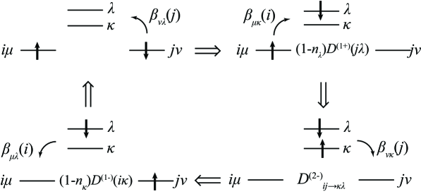
Figure 6: Sequence of configurations relevant to the matrix elements of type (f) as contributing to the effective exchange interaction in the case (i). The configurations in the upper right and lower left corners belong to the outer subspace $\mathrm{Im}Q^{(1-)}$ - that formed from the model space configurations by the MLCT states/processes, that in the lower right corner belongs to the outer subspace $\mathrm{Im}Q^{(2-)}$ - that formed from the model space configurations by the (ML)²CT states/processes. Other notation is as in Fig. 1.

Further contributions of the fourth order in $H_{r}$ come from the ionizing components of the effective operator $H_{rr}$. These are the averages of the form: $\left\langle\Phi_{L}\left|PH_{rr}^{(2\pm)}QR(E)QH_{rr}^{(2\mp)}P\right|\Phi_{L}\right\rangle$. Corresponding configurations are depicted in Figs. 5, 6. The configurations of that type (specifically with the two electrons extracted from an l-MO, but not those with two electrons added to one of them) have been used,[42] but not systematically. We as usually depart from the action of the perturbation operator on the ligand ground state $\left|\Phi_{L}\right\rangle$. For $H_{rr}^{(2+)}$ it reads:

$$H_{rr}^{(2+)}\left|\Phi_{L}\right\rangle=\sum\limits_{\mu i\lambda\sigma}\sum\limits_{\nu j\kappa\tau}\beta_{\mu\lambda}(i)\beta_{\nu\kappa}(j)D^{(1+)}(j\kappa)d_{\mu\tau}^{+}(i)d_{\nu\tau}^{+}(j)a_{\lambda\sigma}a_{\kappa\tau}\left|\Phi_{L}\right\rangle.$$

Multiplying this by the resolvent which in the $\mathrm{Im}Q^{(2+)}$ subspace contains as multipliers the projection operators to doubly ionized ligand states
$a_{\lambda^{\prime}\sigma^{\prime}}a_{\kappa^{\prime}\tau^{\prime}}\left|\Phi_{L}\right\rangle\left\langle\Phi_{L}\right|a_{\kappa^{\prime}\tau^{\prime}}^{+}a_{\lambda^{\prime}\sigma^{\prime}}^{+}$. One can expect that the singlet and triplet ionized states contribute separately. We, however, following[42] concentrate first of all on the states where each l-MO is doubly ionized in either sense. That is we take into account only the terms with $\lambda^{\prime}=\kappa^{\prime}$. In this case $\tau^{\prime}=-\sigma^{\prime}$ holds and inserting the corresponding energy denominator $D^{(2+)}(\lambda^{\prime}\kappa^{\prime}\rightarrow ij)=D^{(2+)}(\kappa^{\prime}\kappa^{\prime}\rightarrow ij)$ which is given by

$$D^{(2+)}(\lambda\kappa\rightarrow ij) = I_{\lambda}-A\left(i\right)-g_{\lambda}\left(i\right)$$ (54)

$$+ I_{\kappa}-A\left(j\right)-g_{\kappa}\left(j\right)$$

$$- g_{\kappa}\left(i\right)-g_{\lambda}\left(j\right)+g_{\kappa\lambda}+g_{ij}$$

$$D^{(2-)}(ij\rightarrow\lambda\kappa) = I\left(i\right)-A_{\lambda}-g_{\lambda}\left(i\right)$$

$$+ I\left(j\right)-A_{\kappa}-g_{\kappa}\left(j\right)$$

$$- g_{\kappa}\left(i\right)-g_{\lambda}\left(j\right)+g_{\kappa\lambda}+g_{ij}$$

we arrive to

$$\sum\limits_{\mu^{\prime}i^{\prime}\lambda^{\prime}\sigma^{\prime}}\sum\limits_{\nu^{\prime}j^{\prime}\kappa^{\prime}\tau^{\prime}}\sum\limits_{\mu i\lambda\sigma}\sum\limits_{\nu j\kappa\tau}\beta_{\mu^{\prime}\lambda^{\prime}}(i^{\prime})\beta_{\nu^{\prime}\kappa^{\prime}}(j^{\prime})\beta_{\mu\lambda}(i)\beta_{\nu\kappa}(j)D^{(2+)}(\lambda^{\prime}\kappa^{\prime}\rightarrow ij)$$

$$D^{(1+)}(j^{\prime}\kappa^{\prime})D^{(1+)}(j\kappa)d_{\mu^{\prime}\tau^{\prime}}(i^{\prime})d_{\nu^{\prime}\tau^{\prime}}(j^{\prime})d_{\mu\tau}^{+}(i)d_{\nu\tau}^{+}(j)\left\langle\Phi_{L}\left|a_{\lambda^{\prime}\sigma^{\prime}}^{+}a_{\kappa^{\prime}\tau^{\prime}}^{+}a_{\lambda\sigma}a_{\kappa\tau}\right|\Phi_{L}\right\rangle$$ (55)

which contains the averages of the form $\left\langle\Phi_{L}\left|a_{\kappa^{\prime}\tau^{\prime}}^{+}a_{\lambda^{\prime}\sigma^{\prime}}^{+}a_{\lambda\sigma}a_{\kappa\tau}\right|\Phi_{L}\right\rangle$ over the one-determinant l-system ground state which are equal to $\left(\delta_{\lambda\lambda^{\prime}}\delta_{\kappa\kappa^{\prime}}\delta_{\sigma\sigma^{\prime}}\delta_{\tau\tau^{\prime}}-\delta_{\kappa\lambda^{\prime}}\delta_{\lambda\kappa^{\prime}}\delta_{\tau\sigma^{\prime}}\delta_{\sigma\tau^{\prime}}\right)n_{\kappa}n_{\lambda}$. Inserting this latter value of the averages and reducing the summation we arrive to the generalization of the expressions[42] suitable for programming:

$$\sum\limits_{\mu i}\sum\limits_{\nu j}\sum_{\kappa}\left[\beta_{\mu\kappa}(i)\beta_{\nu\kappa}(j)\right]^{2}D^{(2+)}(\kappa\kappa\rightarrow ij)D^{(1+)}(j\kappa)\left[D^{(1+)}(j\kappa)+D^{(1+)}(i\kappa)\right] (e)$$ (56)

which contributes to the same exchange matrix elements as the Weihe-Güdel cases (i) and (ii) (see Table D.2).

D.2 MMCT contributions to the effective spin operator

Finally we are in a position to get the estimates of the contributions to the effective exchange parameters of the spin Hamiltonian which is in a way an approximation to the exact eq. (53). We do this in a line with the prescriptions of Ref. [40] which are based on the fact that if it goes about a binuclear i.e. the simplest possible PTMC (a dimer in the terminology of Refs. [39, 40, 42, 43]) each of the terms in eqs. (53), (55) yields a contribution to the energy which is proportional to $S(S+1)$ where $S$ is the total spin of the dimer. These contributions when summed up produce the sought coefficient at the product $\hat{S}_{1}\hat{S}_{2}$ which is the effective exchange parameter. The situation in a PTMC with more than two TMI’s is more complicated; we consider it elsewhere. For the dimer the derivation evolves as follows: each of the terms in eq. (53) describes a process in which an electron is taken from one of the d-orbitals of one of the TMI’s and put to one of the d-orbitals in another TMI. These orbitals are run over by the subscripts $\mu,\nu$. It is only possible in high-symmetry systems when an electron taken from one orbital finally lands in another orbital degenerate with the original one. However for PTMC (unless it goes about the cuts from highly symmetrical solids) one cannot count on the representaion with the dimension higher than two. We, however, assume that the symmetry is low enough so that no spatially degenerate states can appear. With this precaution we rewrite the relevant part of the effective operator eq. (53). The expression eq. (53) represents in fact an effective interaction between electrons in the d-shells of the PTMC. The terms off-diagonal with respect to orbital indices $\mu\mu^{\prime}$ or $\nu\nu^{\prime}$ generate correlated transitions between the different crystal field states in the respective d-shells. However, the magnetic interactions which are our main goal and thus the crystal field excitations are not welcome. In fact these terms lead to various anisotropic contributions, but we for the time being concentrate on the isotropic ones. In order to avoid excitations other than magnetic in the ground state manifold one has to set $\left(\mu^{\prime}i\right)=\left(\mu i\right);\left(\mu^{\prime}j\right)=\left(\nu j\right);\left(\nu^{\prime}j\right)=\left(\nu j\right);\left(\nu^{\prime}i\right)=\left(\mu i\right)$ in the above expression and to change $\left(\mu i\right)\leftrightarrow\left(\nu j\right)$ in the terms of the type (b) and (d).

$$\left\langle\Phi_{L}\left|\mathfrak{P}H_{rr}^{(0)}\mathfrak{Q}\mathfrak{R}(\mathfrak{E})\mathfrak{Q}H_{rr}^{(0)}\mathfrak{P}\right|\Phi_{L}\right\rangle\approx \sum\limits_{i\neq j}\sum\limits_{\mu\nu}$$

$$\left\{\left(\sum_{\kappa}\beta_{\mu\kappa}(i)\beta_{\nu\kappa}(j)D^{(1+)}(j\kappa)n_{\kappa}\right)\right. \left(\sum_{\lambda}\beta_{\mu\lambda}(i)\beta_{\nu\lambda}(j)D^{(1+)}(j\lambda)n_{\lambda}\right)\mathfrak{D}_{i\rightarrow j}^{(0)} (a)$$

$$\sum_{\tau\tau^{\prime}}d_{\mu\tau^{\prime}}^{+}(i)d_{\nu\tau^{\prime}}(j)\mathcal{\mathbb{O}}_{-}^{i}\mathcal{\mathbb{O}}_{+}^{j}d_{\nu\tau}^{+}(j)d_{\mu\tau}(i)$$

$$-\left(\sum_{\kappa}\beta_{\nu\kappa}(j)\beta_{\mu\kappa}(i)D^{(1+)}(i\kappa)n_{\kappa}\right) \left(\sum_{\lambda}\beta_{\mu\lambda}(i)\beta_{\nu\lambda}(j)D^{(1-)}(j\lambda)\left(1-n_{\lambda}\right)\right)\mathfrak{D}_{i\rightarrow j}^{(0)} (b)$$ (57)

$$\sum_{\tau\tau^{\prime}}d_{\nu\tau^{\prime}}^{+}(j)d_{\mu\tau^{\prime}}(i)\mathcal{\mathbb{O}}_{+}^{i}\mathcal{\mathbb{O}}_{-}^{j}d_{\mu\tau}^{+}(i)d_{\nu\tau}(j)$$

$$-\left(\sum_{\kappa}\beta_{\nu\kappa}(j)\beta_{\mu\kappa}(i)D^{(1-)}(i\kappa)\left(1-n_{\kappa}\right)\right) \left(\sum_{\lambda}\beta_{\mu\lambda}(i)\beta_{\nu\lambda}(j)D^{(1+)}(j\lambda)n_{\lambda}\right)\mathfrak{D}_{i\rightarrow j}^{(0)} (c)$$

$$\sum_{\tau\tau^{\prime}}d_{\mu\tau^{\prime}}^{+}(i)d_{\nu\tau^{\prime}}(j)\mathcal{\mathbb{O}}_{-}^{i}\mathcal{\mathbb{O}}_{+}^{j}d_{\nu\tau}^{+}(j)d_{\mu\tau}(i)$$

$$+\left(\sum_{\kappa}\beta_{\mu\kappa}(i)\beta_{\nu\kappa}(j)D^{(1-)}(j\kappa)\left(1-n_{\kappa}\right)\right) \left(\sum_{\lambda}\beta_{\mu\lambda}(i)\beta_{\nu\lambda}(j)D^{(1-)}(j\lambda)\left(1-n_{\lambda}\right)\right)\mathfrak{D}_{i\rightarrow j}^{(0)} (d)$$

$$\left.\sum_{\tau\tau^{\prime}}d_{\nu\tau^{\prime}}^{+}(j)d_{\mu\tau^{\prime}}(i)\mathcal{\mathbb{O}}_{+}^{i}\mathcal{\mathbb{O}}_{-}^{j}d_{\mu\tau}^{+}(i)d_{\nu\tau}(j)\right\}.$$

Further classification is based on the fact[40, 42, 43] that averages of the terms entering the above expression depend on the total spin state of PTMC and on the way they are composed of the states with definite spins of the involved i-th and $j$-th d-shells and through this from the occupancy relations between the involved orbitals. The required calculations based on the work[76] had been performed.[40] Specifically, each of the terms in eq. (57) gives rise to an electron redisribution process (MMCT) starting and ending in a state of the total spin $S$ with i-th and j-th d-shells occurring in the states with the spins $S(i)$ and $S(j)$. In the intermediate MMCT state belonging to the configuration subspace $\mathrm{Im}\mathcal{\mathbb{O}}_{+}^{i}\mathcal{\mathbb{O}}_{-}^{j}\prec\mathrm{Im}\mathfrak{Q}$ the spins of the involved d-shells can have only one of four combinations of the spin values $S(i)\pm\frac{1}{2};S(j)\pm\frac{1}{2}$ which however may realize or not depending on the availability of electrons to be involved in the specific MMCT process or of free space in the d-shells at hand. The results are given in Table D.2 which is derived[40] under an additional assumption that the total spin of an individual d-shell always goes down whenever a half-filled orbital is involved in the MMCT process at this particular shell.

Spin dependent factors for the numbers $u_{i}$ of unpaired electrons in the i-th d-shell.

Weihe-Güdel	Change of occupancies	Unpairity	Spin dependent
cases	$\left(\mu i\right)\Rightarrow\left(\nu j\right)$	factors	multipliers
	in the MMCT process	$U(u_{i},u_{j})$
i	$\left[1/2\right]\Rightarrow\left[1/2\right]$	$\frac{2}{u_{i}u_{j}}$	$+1$ $S(i)\rightarrow S(i)-1/2;S(j)\rightarrow S(j)-1/2$
ii	$\left[1/2\right]\Rightarrow\left[0\right]$	$\frac{2}{u_{i}\left(u_{j}+1\right)}$	$\begin{cases}\left(+1\right)&S(i)\rightarrow S(i)-1/2;S(j)\rightarrow S(j)-1/2\\ \left(-1\right)&S(i)\rightarrow S(i)-1/2;S(j)\rightarrow S(j)+1/2\end{cases}$
iii	$\left[1\right]\Rightarrow\left[1/2\right]$	$\frac{2}{\left(u_{i}+1\right)u_{j}}$	$\begin{cases}\left(+1\right)&S(i)\rightarrow S(i)-1/2;S(j)\rightarrow S(j)-1/2\\ \left(-1\right)&S(i)\rightarrow S(i)+1/2;S(j)\rightarrow S(j)-1/2\end{cases}$
iv	$\left[1\right]\Rightarrow\left[0\right]$	$\frac{2}{\left(u_{i}+1\right)\left(u_{j}+1\right)}$	$\begin{cases}\left(+1\right)&S(i)\rightarrow S(i)\pm 1/2;S(j)\rightarrow S(j)\pm 1/2\\ \left(-1\right)&S(i)\rightarrow S(i)\pm 1/2;S(j)\rightarrow S(j)\mp 1/2\end{cases}$

Otherwise inspecting eq. (57) shows that for each pair of the d-states $\mu\nu$ located respectively in the i-th and $j$-th TMIs the electron/hole transfer through the empty/occupied ligand MOs involves formally the same product of the resonance integrals:

$$\beta_{\nu\kappa}(j)\beta_{\mu\kappa}(i)\beta_{\mu\lambda}(i)\beta_{\nu\lambda}(j)$$

which depending on the type of the process (a) - (d) is complemented by a different combination of l-MO occupancy numbers and energy denominators:

$$D^{(1+)}(j\kappa) \mathfrak{D}_{i\rightarrow j}^{(0)} D^{(1+)}(j\lambda)\times n_{\kappa}n_{\lambda} (a)$$

$$-D^{(1+)}(j\kappa) \mathfrak{D}_{i\rightarrow j}^{(0)} D^{(1-)}(i\lambda)\times n_{\kappa}\left(1-n_{\lambda}\right) (b)$$ (58)

$$-D^{(1-)}(i\kappa) \mathfrak{D}_{i\rightarrow j}^{(0)} D^{(1+)}(j\lambda)\times \left(1-n_{\kappa}\right)n_{\lambda} (c)$$

$$D^{(1-)}(i\kappa) \mathfrak{D}_{i\rightarrow j}^{(0)} D^{(1-)}(i\lambda)\times \left(1-n_{\lambda}\right)\left(1-n_{\kappa}\right) (d)$$

Either of the MMCT processes (a) - (d) as classified according to the ligand MOs involved contributes to the cases (i) - (iv) classified according to the type of the MMCT process involved. This allows to establish the correspondence between the general form of the contributions to the effective exchange parameters and their specific forms and cases as given in Table 4.

Table 4: Correspondence between terms[42, 43] and eqs. (56), (57), (58).

Factor in Refs. [42, 43]	Factor in this work
$V_{a}$	$n_{\lambda}\beta_{\mu\lambda}(i)$ or $n_{\kappa}\beta_{\mu\kappa}(i)$
$V_{a}^{*}$	$\left(1-n_{\lambda}\right)\beta_{\mu\lambda}(i)$ or $\left(1-n_{\kappa}\right)\beta_{\mu\kappa}(i)$
$\Delta_{A}$	$D^{(1+)}(i\kappa)n_{\kappa}$
$\Delta_{A}^{*}$	$D^{(1-)}(i\kappa)\left(1-n_{\lambda}\right)$
$U_{AB}$	$\mathfrak{D}_{i\rightarrow j}^{(0)}$
$V_{b}$	$n_{\lambda}\beta_{\nu\lambda}(j)$ or $n_{\kappa}\beta_{\mu\kappa}(j)$
$V_{b}^{*}$	$\left(1-n_{\lambda}\right)\beta_{\nu\lambda}(j)$ or $\left(1-n_{\kappa}\right)\beta_{\mu\kappa}(j)$
$\Delta_{B}$	$D^{(1+)}(j\lambda)n_{\lambda}$
$\Delta_{B}^{*}$	$D^{(1-)}(j\lambda)\left(1-n_{\lambda}\right)$
$U_{BA}$	$\mathfrak{D}_{j\rightarrow i}^{(0)}$
$\Delta_{AB}$	$D^{(2+)}(\kappa\kappa\rightarrow ij)$

It is remarkable that the overall effect of these contributions cannot be represented as one of the effective hopping of electrons between the d-shells.

D.3 Correlated double ionization contributions to the effective spin operator

These terms stem from the averages $\left\langle\Phi_{L}\left|PH_{rr}^{(2+)}Q^{(2+)}R^{(2+)}(E)Q^{(2+)}H_{rr}^{(2+)}P\right|\Phi_{L}\right\rangle$ and are given by eqs. (55), (56). The terms within the $(2-)$-segment are processed analogously and result in

$$\sum\limits_{\mu i}\sum\limits_{\nu j}\sum_{\kappa}\left[\beta_{\mu\kappa}(i)\beta_{\nu\kappa}(j)\right]^{2}D^{(2-)}(ij\rightarrow\kappa\kappa)D^{(1-)}(j\kappa)\left[D^{(1-)}(j\kappa)+D^{(1-)}(i\kappa)\right].$$

Figures

References

- [1] H.A. Bethe. Ann. Physik, 1929, 3:133–206.
- [2] J.H. Van Vleck. The Theory of Electric and Magnetic Susceptibilities. Oxford: Univ. Press, 1932. 384 p.; Phys. Rev. 1934, 45, 405; J. Chem. Phys. 1941, 9, 85.
- [3] C.J. Milios, A. Vinslava, W. Wernsdorfer, S. Moggach, S. Parsons, S.P. Perlepes, G. Christou, E.K. Brechin. J. Am. Chem. Soc. 129, 2754 (2007)
- [4] S. Carretta, T. Guidi, P. Santini, G. Amoretti, O. Pieper, B. Lake, J. van Slageren, F. El Hallak, W. Wernsdorfer, H. Mutka, M. Russina, C.J. Milios, E.K. Brechin, Phys. Rev. Lett. 100, 157203 (2008)
- [5] A. Müller, M. Luban, C. Schröder, R. Modler, P. Kögerler, M. Axenovich, J. Schnack, P. Canfield, S. Bud’ko, N. Harrison, Chem. Phys. Chem. 2, 517 (2001)
- [6] U. Kortz, A. Müller, J. van Slageren, J. Schnack, N.S. Dalal, M. Dressel. Cood. Chem. Rev. 253 (2009) 2315-2327.
- [7] P. De Loth, P. Cassoux, J.-P. Daudey, J.-P. Malrieu. J. Am. Chem. Soc., 1981, 103, 4007-4016.
- [8] M.F. Charlot, M. Verdaguer, Y. Journaux, P. De Loth, J.-P. Daudey, Inorg. Chem., 1984, 23 (23), 3802-3808.
- [9] P. de Loth, J.-P. Daudey, H. Astheimer, L. Walz, W. Haase. J. Chem. Phys. 82, 5048 (1985).
- [10] K. Fink, R. Fink, V. Staemmler. Inorg. Chem. 1994, 33, 6219.
- [11] C. Wang, K. Fink, V. Staemmler. Chem. Phys. 1995, 192, 25.
- [12] E. Ruiz, et al. J. Comp. Chem. 20: 1391-1400, 1999
- [13] E. Ruiz. Struct. Bond. (2004) 113:71–102.
- [14] M.B. Darkhovskii, A.V. Soudackov, A.L. Tchougréeff. Theor. Chem. Acc. 114 (2005) 97-109.
- [15] M.B. Darkhovskii, A.L. Tchougréeff. in Advanced Topics in Theoretical Chemical Physics. J.-P. Julien, J. Maruani, and E. Brändas (eds). Springer. (2006) p. 451-505 (Progress in Theoretical Chemistry and Physics. No 15).
- [16] P.W. Anderson. Phys. Rev. 115 (1959) 2 - 13.
- [17] P.W. Anderson, in Magnetism. Vol. 1. G.T. Rado, H. Suhl Eds. AP, NY (1963); P. W. Anderson: Solid State Phys. 14 (1963) 99.
- [18] J.B. Goodenough. Magnetism and the Chemical Bond. Interscience-Wiley, NY (1963).
- [19] S.V. Vonsovskii, Magnetism. Nauka, Moscow (1971) [in Russian]; S.V. Vonsovsky, Magnetism. Wiley, NY (1974) in two volumes.
- [20] W.A. Harrison. Electronic Structure and the Properties of Solids: The Physics of the Chemical Bond. W.H. Freeman Co San Francisco (1980)
- [21] C.J. Ballhausen. Indroduction to Ligand Field Theory. McGraw Hill, New York, 1962.
- [22] Bersuker I.B. Electronic Structure and properties of Coordination Compounds. Khimiya, Moscow, 1976. [in Russian].
- [23] A.V. Soudackov, A.L. Tchougréeff, I.A. Misurkin. Theor. Chim. Acta 83 (1992) 389-416.
- [24] R. McWeeny. Methods of Molecular Quantum Mechanics (2-nd ed.) Academic, London, 1992.
- [25] P.-O. Löwdin. Perturbation theory and its application in quantum mechanics. Ed. by C.H. Wilcox N.Y.: Wiley, 1966.
- [26] A.L. Tchougréeff. Phys. Chem. Chem. Phys. 1 (1999) 1051-1060.
- [27] A.L. Tchougréeff. J. Struct. Chem. 48 (2007) S39-S62 [in Russian].
- [28] A.L. Tchougréeff. Hybrid Methods of Molecular Modeling. – Monograph. 346 pp. Springer Verlag, 2008.
- [29] A.V. Soudackov, A.L. Tchougréeff, I.A. Misurkin. Zh. Fiz. Khim. 68 (1994) 1256-1264 [Russ. J. Phys. Chem. 68 (1994) 1135].
- [30] A.V. Soudackov, A.L. Tchougréeff, I.A. Misurkin. Zh. Fiz. Khim. 68 (1994) 1264-1270 [Russ. J. Phys. Chem. 68 (1994) 1142].
- [31] A.V. Soudackov, A.L. Tchougréeff, I.A. Misurkin. Int. J. Quant. Chem. 57 (1996) 663-671.
- [32] A.V. Soudackov, A.L. Tchougréeff, I.A. Misurkin. Int. J. Quant. Chem. 58 (1996) 161-173.
- [33] A.L. Tchougréeff. Khim. Fiz. 17 (1998) No 6, 163-167 [Chem. Phys. Reports. 17 (1998) No 6, 1241].
- [34] M.B. Darkhovskii, A.L. Tchougréeff. Khim. Fiz. 18 (1999) No 1, 73-79 [Chem. Phys. Reports. 18 (1999) No 1, 149].
- [35] A.L. Tchougréeff. in Molecular Modeling and Dynamics of Bioinorganic Systems. L. Banci, P. Comba (eds.) Kluwer, Dordrecht (1997).
- [36] M.B. Darkhovskii, M.G. Razumov, I.V. Pletnev, A.L. Tchougréeff. Int. J. Quant. Chem. 88 (2002) 588-605.
- [37] M.B. Darkhovskii, I.V. Pletnev, A.L. Tchougréeff. J. Comp. Chem. 24 (2003) 1703-1719.
- [38] M.B. Darkhovskii, A.L. Tchougréeff. J. Phys. Chem. A 108 (2004) 6351-6364.
- [39] H. Weihe, H.U. Güdel. Chem. Phys. Lett. 261 (1996) 123-128
- [40] H. Weihe, H.U. Güdel. Inorg. Chem. 1997, 36, 3632-3639.
- [41] H. Weihe, H.U. Güdel. JACS 120 (1998) 2870-2879.
- [42] H. Weihe, H.U. Güdel, H. Toftlund. Inorg. Chem. 2000, 39, 1351-1362.
- [43] H. Weihe, H.U. Güdel. Comm. Inorg. Chem. 22 (2000), 75-103
- [44] F. Tuczek, E.I. Solomon. Inorg. Chem., 1993, 32 (13), pp 2850–2862.
- [45] C.A. Brown, G.J. Remar, R.L. Musselman, E.I. Solomon. Inorg. Chem., 1995, 34 (3), pp 688–717.
- [46] P.R. Surján. Second Quantized Approach to Quantum Chemistry. Springer, Heidelberg, 1989.
- [47] C.K. Jørgensen. Progr. Inorg. Chem. 1964, 4, 73; Adv Chem Phys 1963, 5, 33.
- [48] C.K. Jørgensen. Absorption Spectra and Chemical Bonding in Complexes. Pergamon Press, Oxford, 1962; Jørgensen, C.K. Modern aspects of ligand field theory; North-Holland: Amsterdam, 1971.
- [49] Lever A.B.P. Inorganic Electronic Spectroscopy; Elsevier: Amsterdam, 1984.
- [50] A.L. Tchougréeff, R. Dronskowski. Int. J. Quant. Chem. 109 (2009) 2606-2621.
- [51] D. Rinaldi, Comput. Chem., 1 (1976) 109; ; with corrections as suggested in: I. Mayer, M. Révész, Comput. Chem., 6 (1982) 153; Korsunov, V.A., Chuvylkin. N.D., Zhidomirov, G.M. Kazanskii. V.B. (1978) Kinetika i Kataliz 19, 1152 [in Russian]; A. Mitkov (1988) private communication; A.L. Tchougréeff, A.Yu. Cohn, I.A. Misurkin (1989), unpublished.
- [52] M. Yevitz, J.A. Stanko. J. Am. Chem. Soc. 93 (1971) 1512.
- [53] B.G. Gafford, R.A. Holwerda, H.J. Schugar, J.A. Potenza. Inorg. Chem. 27 (1988) 1126
- [54] B.G. Gafford, R.E. Marsh, W.P. Schaefer, J.H. Zhang, C.J. O’Connor, R.A. Holwerda. Inorg. Chem. 29 (1990) 4652.
- [55] N.K. Dalley, X. Kou, C.J. O’Connor, R.A. Holwerda. Inorg.Chem. 35 (1996) 2196.
- [56] S. M. Jorgensen, J. Prakt. Chem., 25, 321, 398 (1882).
- [57] M. Epple, W. Massa. Z. Anorg. Allg. Chem. 1978, 444, 47.
- [58] W. Clegg, Acta Cryst. B 1976, 32, 2907.
- [59] G. Friedrich, H. Fink, H. J. Seifert, Z. Anorg. Allg. Chem. 1987, 548, 141.
- [60] S. Mossin, H. Weihe. Struct. Bonding 106 (2004) 173–180.
- [61] C.C. Ou, R.G. Wollmann, D.N. Hendrickson, J.A. Potenza, H.J. Schugar. J. Am. Chem. Soc. 100 (1978) 4717.
- [62] P. Chaudhuri, K. Wieghardt, B. Nuber, J. Weiss. Angew. Chem., Int. Ed. 24 (1985) 778. also DIBWUG
- [63] W.H. Armstrong, S.J. Lippard. J. Am. Chem. Soc. 106 (1984) 4632.
- [64] J.B. Vincent, J.C. Huffman, G. Christou, Q. Li, M.A. Nanny, D.N. Hendrickson, R.H. Fong, R.H. Fish. J. Am. Chem. Soc. 110 (1988) 6898.
- [65] P.N. Turowski, W.H. Armstrong, S. Liu, S.N. Brown, S.J. Lippard, Inorg. Chem. 33 (1994) 636.
- [66] P. Fulde. Electron Correlations in Molecules and Solids. Springer-Verlag, Berlin, Heidelberg, New York 1991.
- [67] M. Hamermesh. Group Theory and Its Application to Physical Problems. Dover Publications Inc., NY, 1962.
- [68] A.M. Oleś, G. Stollhoff. Phys. Rev. B, 29 (1984) 314-327.
- [69] A.M. Oleś. Phys. Rev. B 28 (1983) 327 - 339.
- [70] L. Kleinman, K. Mednick. Phys. Rev. B 24 (1981) 6880 - 6888.
- [71] E.U. Condon and G.H. Shortley, Theory of Atomic Spectra; Cambridge, 1951.
- [72] J. A. Pople and D. L. Beveridge, Approximate Molecular Orbital Theory, McGraw-Hi& New York, 1970.
- [73] Clack DW, Hush NS, Yandle SR (1972) J Chem Phys 57:3503
- [74] Bacon AD, Zerner MC (1979) Theor Chim Acta 53:21
- [75] Böhm MC, Gleiter R (1980) Theor Chim Acta 57:315; ibid. (1981) 59:127; Böhm MC ibid (1981) 60:233
- [76] Damhus, T. Mol. Phys. 1983, 50, 497.