chapter [1.5em] 1em *[1pc]. section [3.5em] 2.3em *[1pc]. subsection [4.5em] 2.3em *[1pc]. subsubsection [5.5em] 2.3em *[1pc].

A Proposal for the Muon Piston

Calorimeter Extension (MPC-EX)

to the PHENIX Experiment at RHIC

Brookhaven National Laboratory

Relativistic Heavy Ion Collider

Introduction and Executive Summary

The Muon Piston Calorimeter (MPC) Extension, or MPC-EX, is a Si-W preshower detector that will be installed in front of the existing PHENIX MPC’s. This detector consists of eight layers of Si “minipad” sensors interleaved with tungsten absorber and enables the identification and reconstruction of $\pi^{0}$ mesons at energies up to $\sim$80 GeV.

The MPC and MPC-EX sit at forward rapidities ($3.1<\eta<3.8$) and are uniquely positioned to measure phenomena related to either low-x partons (in the target hadron or nucleus) or high-x partons (in the projectile nucleon or nucleus). We propose to use the power and capabilities of the MPC-EX to make critical new measurements that will elucidate the gluon distribution at low-x in nuclei as well as the origin of large transverse single spin asymmetries in polarized p+p collisions.

The collision of deuterons and Au nuclei at RHIC offers an exciting window into the initial state of HI collisions as well a probe of partonic phenomena in nuclei that are interesting in their own right. Measurements of the production of $\pi^{0}$ mesons at forward rapidities (in the deuteron direction) at RHIC have already shown a suppression that could be interpreted in terms of partonic shadowing or the formation of a condensate of gluons below a saturation scale (the Color Glass Condensate, or CGC). The MPC-EX will be able to extend these measurements to a new kinematic regime, and through correlations, down to a partonic x of $10^{-3}$. Such measurements will provide high statistics data that can be further used to constrain models of the gluon saturation at low-x in nuclei. However, measurements of hadrons will be limited by uncertainties in the $\pi^{0}$ fragmentation functions and contamination and dilution from partonic processes other than those of interest.

With the capability of the MPC-EX to reconstruct and reject $\pi^{0}$ mesons (as well as other hadronic sources of photons) at very high energies comes the capability to separate prompt (direct and fragmentation) photons from other sources of photons. Direct photons are extremely interesting as a complimentary observable to hadronic measurements. At leading order the direct photon kinematics are much more easily related to the parton kinematics because there is no smearing due to fragmentation. However, a measurement of direct photons is more difficult experimentally and will involve different systematic errors when compared to measurements of hadrons.

We propose to investigate gluon saturation in nuclei at low-x through the measurement of $R_{dAu}$ for $\pi^{0}$ mesons and direct photons. These measurements will provide strong constraints on existing models of the gluon PDF in nuclei, such as the EPS09 PDF sets. These measurements will be timely and competitive with measurements from the LHC. The timing of a future d+Au run at the LHC is not known, although it is certainly under discussion. Both ATLAS and CMS have electromagnetic calorimeters in the forward region. However, a crucial element of the direct photon measurement is the ability of the MPC-EX at RHIC to measure relatively low p_T direct photons to measure R_G at low Q² where the suppression is strongest, which is not accessible at the LHC.

The large transverse single-spin asymmetries observed in polarized p+p collisions at RHIC are believed to be related to either initial or final state effects that originate primarily in the valence region of the projectile nucleon (the Sivers or transversity distributions in the TMD approach, or parton correlations in a collinear factorized framework). While data in semi-inclusive deep-inelastic scattering has been used to constrain these effects, the situation is more complicated in p+p collisions due to the presence of both strong initial- and final-state corrections arising from the soft exchange of gluons.

A key issue in making progress in the theoretical understanding of transverse spin asymmetries in p+p collisions are measurements that can elucidate the origin of the single hadron asymmetries. One approach is to measure the single spin asymmetry $A_{N}$ for prompt photons, which is dominated by initial state correlations between partonic motion and proton spin. Because of the ability of the MPC-EX to reject high momentum $\pi^{0}$ mesons as well as measure the asymmmetry of background contributions from $\pi^{0}$ and $\eta$ mesons, the SSA of prompt photons can be measured with good precision in 200 GeV transversely polarized p+p collsions.

Another approach is to directly measure the asymmetry in the fragmentation of spin-polarized quarks that arise from the hard scattering of partons in a polarized p+p collision. In addition to providing fine-grained information on the development of electromagnetic showers, the MPC-EX is also capable of tracking minimum ionizing particles (charged hadrons) that do not shower in the detector. While we do not have an energy or momentum measurement for these hadrons, this capability can be exploited to reconstruct a proxy for the jet axis for a fragmenting parton. Because $\pi^{+}$ and $\pi^{-}$ hadrons, the dominant charged particle species in the jet, exhibit a roughly equal and opposite transverse spin asymmetry, the effect of the asymmetry on the determination of the jet axis is minimized. This jet axis can then be used to correlate the azimuthal angle of $\pi^{0}$ mesons around the jet axis, with respect to the spin direction. An asymmetry measured in this way would arise from the combination of quark transversity and the Collins spin-dependent fragmentation function (in the TMD framework). Measurements made with the MPC-EX would be sensitive to this source of the single particle transverse spin asymmetry if it made up as little as $\sim$27% of the single-particle transverse spin asymmetry.

The structure of this proposal is organized as follows. In the first chapter we highlight the MPC-EX physics case for cold nuclear matter and nucleon spin. The second chapter describes the hardware design of the MPC-EX and its integration into the existing PHENIX detector. In the third chapter we detail the simulations completed to characterize the performance of the MPC-EX detector for the reconstruction of electromagnetic showers and the separation of direct photons from other sources. In the last two sections of this chapter we detail a full simulation of two key physics observables in the MPC-EX, the direct photon and the measurement of azimuthal asymmetries in fragmentation. Finally, we conclude with chapters on the budget and management of the MPC-EX project. Appendix A contains additional information on events rates, cross sections, and triggering schemes that were used to make the projections in the third chapter.

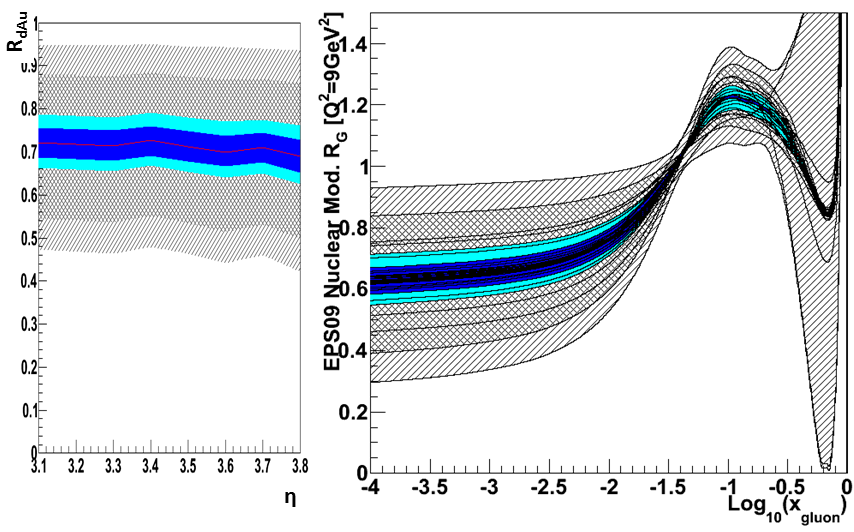
Figure 1: EPS09 exclusion plots in R_dAu (left) and R_G (right). The outer hatched lines are the 90% confidence level envelope of all the EPS09 curves. The light blue areas represent the 90% confidence level limits of the simulated measurement, while the dark blue represent the 1$\sigma$ limits. The nominal value is taken as the central EPS09 curve. See Section 3.4 for details.

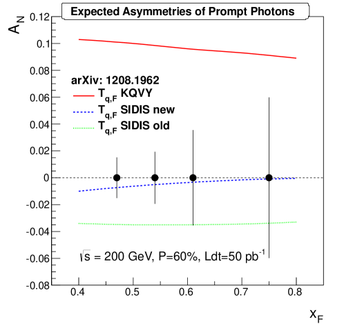
Figure 2: Projected sensitivity for the prompt photon single spin asymmetry with the MPC-EX assuming an integrated luminosity of 50 pb^-1 and 60% beam polarization at $\sqrt{s}=200$ GeV. The sensitivities are shown compared to calculations in the collinear factorized approach  [44, 40] using a direct extraction of the quark-gluon correlation function from polarized $p+p$ data (upper solid curve), compared to the correlation function derived from SIDIS extractions (lower dotted and dashed curves). See Section 3.5 for details.

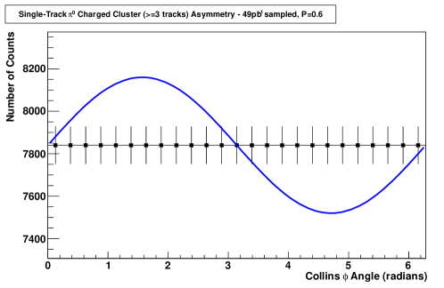
Figure 3: Anticipated statistics as a function of Collins angle for 49 $pb^{-1}$ sampled luminosity and average polarization of 60% using single-track $\pi^{0}$’s correlated with a jet axis determined by three or more charged particles. The blue curve is the anticipated asymmetry for the data sample from the Monte Carlo, corrected for the beam polarization of 60%. See Section 3.7 for details.

Contents

1. 1 Physics Overview
   1. 1.1 Cold Nuclear Matter
   2. 1.2 Nucleon Spin Structure
2. 2 The MPC-EX Preshower Detector
   1. 2.1 The MPC-EX
   2. 2.2 Detector Design
   3. 2.3 Mechanical Design
   4. 2.4 Electronics and Readout
   5. 2.5 Impact of the MPC-EX on PHENIX
3. 3 Simulations and Physics Observables
   1. 3.1 Electromagnetic Shower Reconstruction
   2. 3.2 EM Shower Reconstruction Performance
   3. 3.3 Direct Photons in the Pythia Monte Carlo
   4. 3.4 Direct Photons
   5. 3.5 Direct Photon $A_{N}$
   6. 3.6 Determination of Jet Axis Proxy
   7. 3.7 $\pi^{0}$ Correlations in Jets
4. J Event Rates
5. K MPC-EX Collaboration

Chapter 1 Physics Overview

In this proposal we focus on two key questions in QCD - the suppression of partons at small-x in nuclei, and how the spin of the nucleon is carried by its constituent partons. Both of these questions address fundamental issues in our understanding of QCD, and measurements with the MPC-EX hold the potential to greatly expand our understanding of the strong nuclear force.

1.1 Cold Nuclear Matter, the Initial State of the sQGP and low-$x$ Physics

1.1.1 Introduction

The behavior of parton distributions in a heavy nucleus such as Au is of interest since they are not simply a superposition of nucleon parton distributions, but display effects related to the nuclear environment. These phenomena vary as a function of patonic longitudinal momentum fraction x. Of particular importance is the gluon distribution at low-x where a variety of models predict strong suppression. Very little is known about the gluon distribution function at x_gluon$<10^{-2}$ (for the rest of this section x_gluon in the heavy nucleus will be referred to as x₂). Figure 1.1 shows a variety of fits to the data of the gluon nuclear modification factor

$$R_{g}^{A}(x,Q^{2})=\frac{f_{g}^{A}(x,Q^{2})}{f_{g}^{proton}(x,Q^{2})}$$

the ratio of the gluon distribution function in a nucleus as compared to the proton. A strong suppression could explain the reduction in p+A collisions relative to p+p collisions of pions and pion pairs at forward rapidity [21, 9] as well as the stronger suppression of $J/\psi$ at forward rapidity as compared to mid-rapidity [7].

Figure 1.1: EPS09 gluon nuclear modification ratio, i.e. the ratio between the gluon PDF in a heavy nucleus (Pb) and in a proton. The lines correspond to the various possibilities which are consistent with world data. At low x, there is virtually no constraint.

The need to understand such effects has taken on a new urgency because of the discovery of the sQGP at RHIC. The measurement of the low-x gluon distribution of the nucleus is the first step in understanding the formation of the sQGP at RHIC. To make a first order estimate, the bulk of the particles at p${}_{T}\sim$ few times the initial temperature ($\sim$ 1 GeV, assuming an initial temperature of 300-600 MeV), are formed from gluons within a nucleus with x${}_{2}<10^{-2}$, precisely where there is little constraint. In addition, with the observation that the matter seen in heavy ion collisions at the LHC is very similar to RHIC, the study of these effects is very timely and important since at forward rapidity we probe the same low-x which is relevant for bulk dynamics at the LHC.

A careful measurement of the gluons in a nucleus would set the initial conditions of the initial entropy and entropy fluctuations which lead to the creation of the sQGP. This in turn would allow for the interpretation of jet and flow measurements in terms of interesting physical quantities, e.g. the sheer and bulk viscosity, diffusion coefficients, the speed of sound, and the jet quenching parameter $\hat{q}$. For creation of the bulk hot-dense matter in A+A collisions, the relevant x is below $10^{-2}$. For x_gluon less than $10^{-2}$, the uncertainty is large, hence the region most necessary for setting the initial state of the sQGP is not well known.

1.1.2 Models including the Color Glass Condensate and EPS09

A variety of physical pictures have been used to model gluons at low-x, or forward rapidity. These fall into several classes. The first class of these models extend pQCD calculations into the non-pertubative regime, via the addition of multiple scattering, coherence or higher twist effects[20]. A second class of models is referred to as the Color Class Condensate (CGC)[49, 46] and assume that the density of gluons is high enough that to first order, they can be treated classically. Quantum corrections are added as a second order effect. In its region of applicability (see Figure 1.2) the CGC is a rigorous QCD calculation with essentially one free parameter - the saturation scale Q_sat, although in practice other parameters or assumptions are invoked in order to make comparisons with experimental data. The two contrasting sorts of models could be two equivalent descriptions of the same phenomena, with one being more appropriate than the other depending on the kinematic range in question. An example of this “duality” is mentioned below in the discussion on transverse momentum dependent gluon distributions and the CGC.

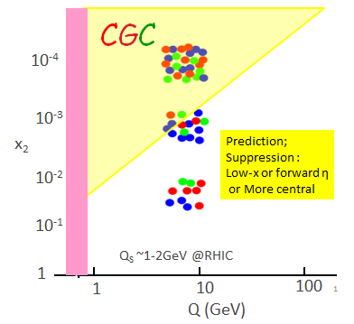
Figure 1.2: A schematic of the CGC region of validity. The plot shows the region of validity (shaded in yellow) as a function of x₂ of the gluon in the Au nucleus in p(d)+Au collisions and Q. The model is valid at high density - which occurs at low-x. For RHIC collisions in Au nuclei, Q${}_{sat}\sim$ 1-2 GeV.

The CGC is valid for very high density systems and is a non-pertubative model. However it requires that the system be weakly interacting and is appropriate only in a regime in which the density is high enough that $\alpha_{S}(Q_{sat})$ is small. Hence, one must establish whether such calculations are applicable at RHIC. The partons which produce the bulk of particles constituting the hot-dense matter at RHIC have an x${}_{2}\sim 10^{-2}$ with the saturation parameter Q_sat in the CGC model $\sim$3T_init. Assuming a value of T${}_{init}\sim$ 300-600 MeV, coming from the PHENIX thermal photon measurement, gives Q${}_{sat}\sim$ 1-2 GeV/c[47]. Pion suppression and correlation data from RHIC[21, 9] at forward rapidities seem to be consistent with the CGC hypothesis, however alternate explanations also may explain the data. Mid-rapidity d+Au pion data at RHIC showed no suppression[11], while it is almost certain that similar data from the LHC will show suppression if the CGC model is correct. If the CGC model is a good description at RHIC, the MPC-EX should be able to measure the parameter Q_sat.

For the purposes of this proposal, a third class of models is used, which are parametrizations of the modification of the gluon distribution function in nuclei, $R_{g}^{A}(x,Q^{2})$. They are obtained by fitting deep-inelastic scattering events, Drell Yan pairs, and RHIC mid-rapidity $\pi^{0}$s[35] and are shown in Figure 1.1. The various lines represent different sets of parametrizations consistent with the data, where the colored region corresponds to the 90% confidence level band. We have added to the EPS09 distributions, a centrality dependence coming from a Glauber model. This class of models does not invoke a physical picture save that the gluons can be legitimately described via x₂, the fraction of the nucleon momentum carried by an individual gluon. It must be stressed that this is simply one model and may not be a good representation of reality; for instance it does not consider the k_T of the parton with respect to in its hadron; it also may be that gluons should not be considered as individual entities, but rather as a collective state.

1.1.3 Direct Photons

Low-x phenomena can be studied using direct photon production at forward rapidities with the MPC-EX. Direct photons can either be used on their own, or they can be correlated with either a pion or a jet opposite in azimuth, to determine x_gluon to leading order with reasonable accuracy. In the CGC model these opposite side correlated particles are suppressed since the recoil is absorbed by the CGC (like the Mossbauer effect). In fact the gluon PDF which gives the distribution of gluons with a fraction x of the nucleon’s momentum, assumes a pQCD like picture. One can use three handles to constrain the theory: the rapidity dependence, centrality dependence (i.e. dependence on Q_sat), and the p_T balance of the recoiling particles. This would yield a centrality and x-dependent set of measurements, allowing a differentiation between various models. The x in question here would be the effective x as measured in the experiment since the variable x₂ is not well defined in the CGC model. The centrality dependence of most pQCD inspired models follows a Glauber distribution, since they are proportional to the thickness function of the nucleus, while for the CGC it is given by the relationship between the saturation parameter Q_sat and the assumed gluon density. Other models, which involve radiative energy loss of quarks traversing cold nuclear matter or absorption, in the case of quarkonia show a non-linear behavior with the nuclear thickness function, uncharacteristic of the Glauber distribution as well.

Present data from d+Au collisions at forward rapidity already shows a suppression of correlated pions[9] in a manner consistent with the CGC. Further theoretical analysis will be necessary to differentiate this interpretation from other nuclear effects. The analysis could also be complicated by the presence of hadron pairs arising from multiparton interactions (MPI)[57] in which case the pairs made by this mechanism would not be probing the gluons at low-x. In addition, PHENIX data on the J/$\psi$ already indicate that cold nuclear matter effects are non-linear. Such effects may be due to final state effects (absorption and energy loss), or initial state effects (e.g. the gluon PDF)[7].

Measurements of hadrons have an ambiguity since they involve a fragmentation function. Direct photons originating from the primary vertex should clarify the situation. Figure 1.3, left shows the basic first-order production diagram for direct photons at forward rapidities. The primary interaction is between a quark in the deuteron and the gluon of interest in the gold nucleus, producing an outgoing photon and jet.

Figure 1.4 shows that the rapidity of the direct photon is directly related to the x₂ of the gluon. Once the direct photon is observed the x₂ can be more accurately determined by including a correlation with a $\pi^{0}$ originating from the opposite side jet. If one assumes that the pseudorapidity of the pion is the same as the pseudorapidity of the jet, one can deduce the x₂ of the gluon to leading order through the relationship

$$x_{2}=p_{T\gamma}(e^{-\eta_{\gamma}}+e^{-\eta_{\pi}})/\sqrt{s}$$

where $p_{T\gamma}$ and $\eta_{\gamma}$ refer to the direct photon, $\eta_{\pi}$ is the pseudorapidity of the $\pi^{0}$ and $\sqrt{s}$ is the nucleon-nucleon center of mass energy. We are currently exploring our capability to measure the complete jet to improve the resolution on x_gluon. Figure 1.5 shows that the measured value of x₂ is nicely correlated with the true x₂ assuming that the first order scattering diagram dominates.

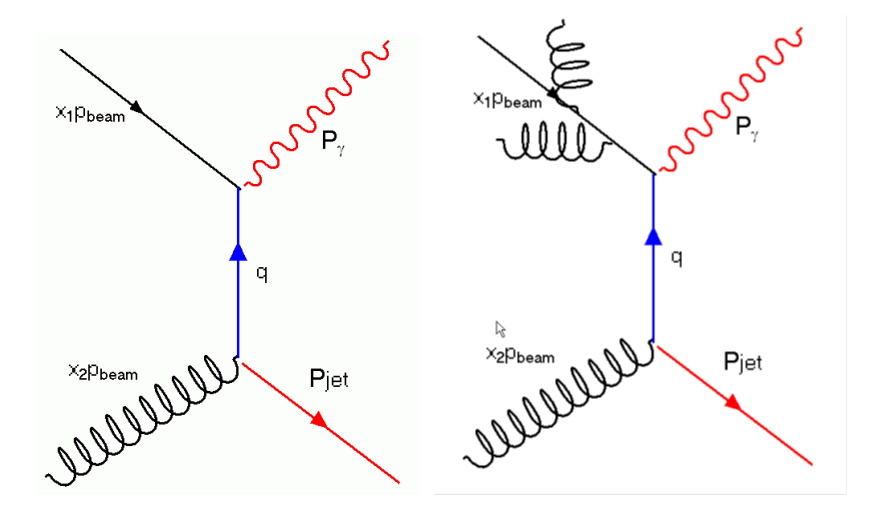
Figure 1.3: Diagrams for the production of direct photons in hadron-hadron collisions. To the left is a first order diagram, the right shows an example of a higher order diagram.

Figure 1.4: Direct photon events: $\eta_{\gamma}$ vs log(x₂), showing the correlation between the pseudorapidity of the photon and x₂. In this figure no correlated hadron is required.

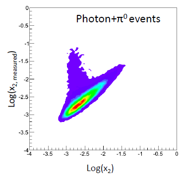
Figure 1.5: x_measured vs x₂ as described in the text. The non-diagonal portion of the plot corresponds to cases in which the detected $\pi^{0}$ was did not give a good estimate of the direction of the outgoing jet, as in the case in which the detected pion was not the leading particle. Such events form about 10% of the events which had a detected photon and $\pi^{0}$ in the MPC-EX.

While not simulated for this proposal, correlations of photons and either hadrons of jets will then allow us to vary the x₂ of the gluon in the following manner. We first require that the direct photon be in the positive rapidity MPC-EX. To reach the lowest values of x, we require the correlated pion to be in the same MPC-EX (and be opposite in azimuth). To reach moderate values of x, we will require a hadron to be stopped in the positive rapidity muon arm (note that we only need the rapidity of the pion, and not its momentum). To reach yet higher values of x, we will require that the pion be in the VTX or central arms. We also plan also to measure the jet angle, using the MPC-EX on both sides, and the new silicon detectors - the VTX at mid-rapidity (installed in 2010) and and the FVTX at forward rapidity (installed in late 2011) to cover essentially the full range in x.

1.1.4 Transverse Momentum Dependent Gluon distributions

An exciting new development [34] has been made in understanding the transverse momentum dependent (TMD) gluon distributions at low-x. Measuring direct photon-jet process in d+Au collisions at low-x, i.e. in the forward direction will give the MPC-EX the opportunity to measure these distributions. These TMD distributions have been shown to be equivalent to the distributions obtained in the CGC frame work. The relationship between these TMD distributions and the spin dependent TMD distributions described in section 1.2, is analogous to the relationship between the ordinary partons distribution functions, e.g. xG(x) and the spin dependent $g^{p}_{1}$. Hence a unified picture is emerging. The MPC-EX is can access both the spin dependent TMD PDFs and the spin independent TMD PDFs. The spin independent TMD PDFs at low-x can be identified as those obtained in the framework of the CGC - i.e. there is a “duality” between the two methods of calculation. This is briefly described in what follows.

Recently work has been done in trying to understand the gluon distributions in cold nuclear matter taking into account the k_T dependence [34]. Models such as EPS09, which we are using to benchmark the measurement, assume “collinear factorization”, i.e. that the physical description of the processes depend only on x₂, the fraction of the proton momentum carried by a parton. This assumes that physical processes do not depend on k_T, the transverse momentum of the partons with respect to the nucleon. The hope was that a similar procedure could be applied to physical processes in which the k_T was an important factor, e.g. in exclusive channels, such as di-jet production, and that cross sections could be factorized into two pieces. The first piece is the hard parton scattering cross section which can be calculated using pQCD. The second piece is the non-pertubative part - the “unintegrated” parton distributions dependent on both x₂ and k_T. These would come from measurements. One of the important assumptions is that the unintegrated PDFs are universal i.e., that the PDFs are the same for all process in question. This “TMD factorization” is analogous to the collinear factorization assumed in the standard k_T independent analysis. Recently it has been shown that TMD factorization is violated in a variety of process (e.g. di-jet production)[61].

In the past decade, these so called unintegrated gluon distributions have been studied in several contexts[41]. The CGC model assumes that for small-x gluons, a regime is reached characterized by the saturation scale Q_sat, below which the process could be calculated semi-classically. The scale Q_sat is the typical transverse momentum of the small-x gluons and is related to the transverse color-charge density - thereby leading to a “condensate” extending over a large transverse portion of nuclear target. Since thick targets, e.g. Au, would lead to a larger transverse charge density, the transition happens at higher-x or lower energy in proton-heavy nucleus collisions than in p+p collisions.

	DIS and DY	SIDIS	hadron in pA	$\gamma$-Jet in pA	Dijet in DIS	Dijet in pA
G(1)	$\times$	$\times$	$\times$	$\times$	$\surd$	$\surd$
G(2)	$\surd$	$\surd$	$\surd$	$\surd$	$\times$	$\surd$

Table 1.1: Processes which are sensitive to G⁽¹⁾ and G⁽²⁾. Direct photon - jet events in pA collisions are sensitive to G⁽²⁾ and dijet events in pA collisions are sensitive to G⁽¹⁾. Taken from [34]. Check marks indicate the gluon distributions relevant to the given process.

Recent progress[34] indicates that TMD factorization can be recovered in the low-x limit if one considers two different unintegrated gluon distributions, G⁽¹⁾ and G⁽²⁾. G⁽¹⁾ can be interpreted as the gluon density. G⁽²⁾ is the dipole gluon distribution and does not have an easily understood physical interpretation. This gluon distribution can be related to the color-dipole cross section evaluated from a dipole of size r_⟂ scattering on the nuclear target. It is G⁽²⁾ that enters into most of the processes of interest - for instance the total cross section (or the structure functions) in DIS, single inclusive hadron production in DIS and pA collisions and Drell-Yan lepton pair production in pA collisions. G⁽¹⁾ can be measured in dijet final states of proton-nucleus collisions, while G⁽²⁾ can be measured in photon-jet final states, thus it is crucial to measure G⁽²⁾, which can be done by the MPC-EX. Table 1.1 shows a variety of processes and the relevant gluon distributions. The MPC-EX will be able measure both of these distributions since the di-jet final state is also within its capabilities.

1.1.5 Measurements Simulated in this Proposal

We have simulated the performance for the basic observable for this physics, namely the single direct photon in forward d+Au events. First we assume that the gluon distributions in Au (Figure 1.1), with the addition of a Glauber model will give us the centrality dependence. Figure 1.4 shows that we will be dominated by events where x${}_{2}\sim 10^{-3}$. We simulate the measurement of R_dAu. In a realistic measurement, one has a contamination of, among other things, fragmentation photons - i.e. photons which fragment off of the outgoing quark legs of the initial hard interaction. These of course, can be reduced using appropriate cuts, however, for completeness we show distributions both with and without these additional sources of photons. A detailed description will be given in Section 3.4. Figure 1.6 shows R_dAu for minimum bias events (left) and central events (right), where we have assumed that there is no attempt to suppress fragmentation photons. The red line shows results where we have assumed the central value of EPS09, the black line shows the results where we have used the parametrization from EPS09 giving the lowest and highest values or R_dAu. Recalling that all the possible pasteurizations given by the EPS09 fits are equally good, we take the envelope of all parametrization to give a one sigma range, shown in light blue. Figure 1.7 shows the same plot, where we have assumed that all fragmentation photons could be eliminated. The final result will lie somewhere between Figure 1.6 and Figure 1.7.

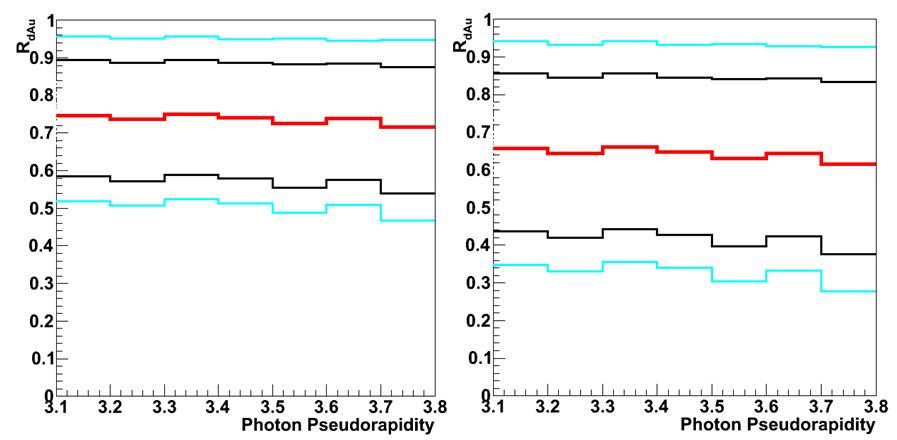
Figure 1.6: Left: R_dAu as simulated in minimum bias events in the MPC-EX vs $\eta$ of the photon, where no attempt is made to suppress fragmentation photons. Red: central value of EPS09. Black: R_dAu obtained when using the least and most suppressed values of the nuclear gluon PDF. Light blue: the envelope of all parametrization to give a one sigma range. Right: same for 0-20% central events.

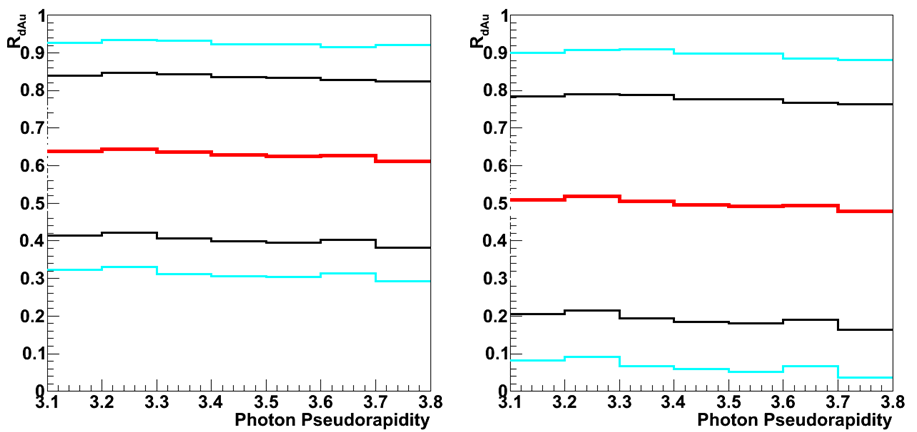
Figure 1.7: Left: R_dAu as simulated in minimum bias events in the MPC-EX vs $\eta$ of the photon assuming no contamination from fragmentation photons. Red: central value of EPS09. Black: R_dAu obtained when using the least and most suppressed values of the nuclear gluon PDF. Light blue: the envelope of all parametrization to give a one sigma range. Right: same for 0-20% Central events.

It must be emphasized, as we conclude this section, that the interpretation of our results will need to be done in close coordination with theorists as in any measurement of a PDF, since, in reality the diagram shown in Figure 1.3, left, is only a first order diagram, and higher orders (e.g Figure 1.3,right) will contribute. What these measurements will give, however, are data to to clarify out understanding of cold nuclear matter and to constrain the initial condition leading to the formation of the sQGP.

1.1.6 Other Experiments

STAR

STAR will not be able to extract direct photon measurements from the Run-8 d+Au data they have already taken with the Forward Pion Detector (FPD), mainly due to the fact that the tower-to-tower gain variations were too large to allow effective triggering. The STAR FPD covers a similar kinematic region as the MPC-EX upgrade and can distinguish $\pi^{0}$ from photon showers up to 50 GeV based on the size of the crystals in the FPD and location from the interaction point. The MPC-EX uses a finely segmented Si-W preshower detector to enable the direct reconstruction of $\pi^{0}$s up to energies $>$80GeV. In many ways the STAR FPD and PHENIX MPC-EX are complimentary and will make complimentary and competitive measurements using different approaches in future d+Au running.

It should be noted that the MPC-EX adds the ability to detect charged particles as well, making possible improved isolation cuts and the correlation of $\pi^{0}$s with respect to a charged cluster axis that is sensitive to the Collins effect in spin-polarized pp collisions. In this way the PHENIX MPC-EX adds significant new capabilities beyond the existing STAR detector.

LHC Experiments

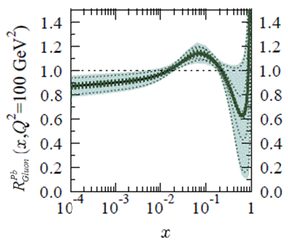
Figure 1.8: EPS09 fits to R${}^{Pb}_{Gluon}$ at a Q² of 100 GeV². The suppression seen at lower Q² is no longer present.

Recently the LHC took a short run with p+Pb collisions. Both ATLAS and CMS have electromagnetic calorimeters in the forward region. However a crucial element of the d+Au measurement is the ability of the MPC-EX to measure relatively low p_T direct photons to measure R_G at low Q². Figure 1.8 shows that for a Q² of 100 GeV² (p_T   10 GeV/c) the suppression of the gluon structure function in nuclei prominent at low Q² is absent. The $\gamma/\pi^{0}$ ratio at LHC energies even at a p_T of 10 GeV/c is greater than 100, making it essentially impossible to measure the direct photon signal.

ALICE does not have electromagnetic calorimeters in the relevant region. Upgrade plans call for the construction of a forward Calorimeter (FOCAL) which may be able to make measurements at low Q². The timescale of the ALICE FOCAL is after the MPC-EX is scheduled to take physics data.

1.2 Nucleon Spin Structure

1.2.1 Nucleon Structure: Transverse Spin Physics

Since the observation of surprisingly large single transverse spin asymmetries (SSAs) in $p^{\uparrow}+p\to\pi+X$ at Fermilab during 1980s and 1990s [5], the exploration of the physics behind the observed SSAs has become a very active research branch in hadron physics, and has played an important role in our efforts to understand QCD and nucleon structure. The field of transverse spin physics has now become one of the hot spots in high energy nuclear physics, generating tremendous excitement on both theoretical and experimental fronts. Fermilab E704’s observation of large SSA [5] initially presented a challenge for QCD theorists and contradicted the general expectation from pQCD of vanishingly small SSA assuming it is originated from a helicity flip of a collinear parton. It was even more startling that the SSA discovered by E704 at $\sqrt{s}$ = 20 GeV did not vanish at all, as expected from pQCD, at the much higher $\sqrt{s}$ of 62.4 GeV and 200 GeV from the BRAHMS [22] and the STAR [4] experiments. The surprisingly large SSA of $\pi^{0}$ mesons observed at STAR, as a function of Feynman $x$, is shown in Figure 1.9. Although theory calculations based on a fit [32] of Sivers Transverse Momentum Dependent parton distributions (TMD) and a twist-3 calculation [48] roughly described the $x_{F}$ dependencies of SSAs, they failed to describe the trend of transverse momentum ($p_{T}$) dependencies of SSA, as shown in Figure 1.10. PHENIX preliminary results of forward “single-cluster” MPC hits (presumably $\pi^{0}$s) SSA $A_{N}$, as in Figure 1.11, also showed similar large size asymmetries. One might question whether the forward reactions are hard enough to apply perturbative QCD, but as shown in Figure 1.12 the cross sections of $p+p\to\pi^{0}+X$ are reasonably described by NLO pQCD [25] as well as by PYTHIA simulations [55]. The existence of large single spin asymmetries at very forward rapidities at RHIC, along with the good theoretical understanding of the unpolarized cross-sections gives hope that transverse spin phenomena in polarized $pp$ collisions at RHIC can be used as a tool to probe the correlation between parton’s transverse motion and the nucleon’s spin in order to provide a 3-dimensional dynamical image of the nucleon.

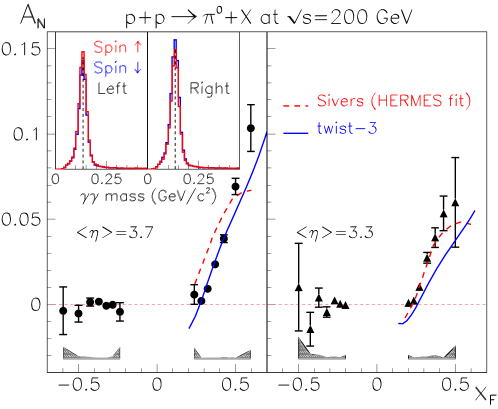
Figure 1.9: Single spin asymmetry $A_{N}$ from $\pi^{0}$ mesons at two different forward rapidity bins ($\langle\eta\rangle=3.3,3.7$) as a function of Feynman $x_{F}$, measured at the STAR experiment from transversely polarized $p+p$ collisions at $\sqrt{s}=200$ GeV [4]. The calculations are: i) a fit [32] of quark Sivers function from HERMES proton Sivers results, ii) a twist-3 calculation [48] as described later in the text. The inset shows examples of the spin-sorted invariant mass distributions. The vertical lines mark the $\pi^{0}$ mass.

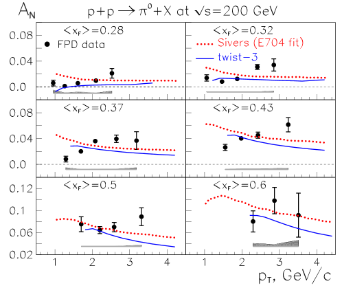
Figure 1.10: Data from STAR: Transverse momentum ($p_{T}$) dependence of Single spin asymmetry $A_{N}$ in fixed $x_{F}$ bins of $\pi^{0}$ mesons production in $p+p$ collisions at $\sqrt{s}=200$ GeV.  [4]. The calculations are: i) a fit [32] of quark Sivers function from HERMES proton Sivers results, ii) a twist-3 calculation [48] as described later in the text.

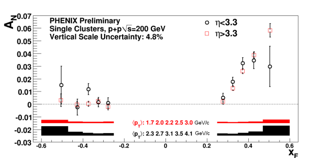
Figure 1.11: PHENIX preliminary results of single spin asymmetry $A_{N}$ vs $x_{F}$ of MPC single-cluster hits (presumably $\pi^{0}$s) in $p+p$ collisions at $\sqrt{s}=200$ GeV.

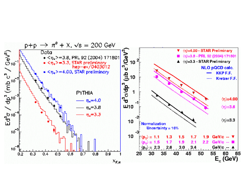
Figure 1.12: Forward inclusive $\pi^{0}$ cross sections measured at the STAR experiment from transversely polarized $p+p$ collisions at $\sqrt{s}=200$ GeV [4]; the average pseudorapidity is $\langle\eta\rangle=3.8$. In the left panel, these results are compared to predictions using PYTHIA [55] as a function of Feynman x; in the right panel they are compared to NLO pQCD calculations as a function of the pion energy.

In order to explain these large single-spin asymmetry phenomena associated with transversely polarized $p+p$ collisions, three basic mechanisms have been introduced (although they can not be clearly separated from each other in inclusive hadron SSA measurements):

1. The “Collins Effect”: a quark’s transverse spin [53] (transversity) generates a left-right bias during the (spin-dependent) quark fragmentation process [30].

2. The “Sivers Effect”: a parton’s transverse motion generates a left-right bias [54].
   The existence of the parton’s Sivers distribution functions ($f^{\perp}_{1T}$), one of the eight leading order Transverse Momentum Dependent parton distributions (TMDs), which is naive T-odd and describes the correlation between parton’s transverse momentum and the nucleon’s transverse spin, allows a left-right bias to appear in the final hadron’s azimuthal distribution. This “TMD factorization approach” is valid in the low $p_{T}$ region ($p_{T}\sim\Lambda_{QCD}\ll Q$).

3. The so-called “twist-3 colinear factorization approach”, valid in high $p_{T}$ region ($p_{T}\gg\Lambda_{QCD}$): a higher twist (twist-3) mechanism in the initial and/or final state [44] that describes SSA in terms of twist-3 transverse-spin-dependent correlations between quarks and gluons. It was shown theoretically that in the intermediate $p_{T}$ region ($\Lambda_{QCD}\ll p_{T}\ll Q$) that overlap between the TMD factorization approach and the twist-3 approach, as in the case of SSAs measured at RHIC $p+p$ collisions, both methods describe the same physics such that a link between the moments of twist-3 three-parton correlation function $T_{q,F}(x,x)$, and the quark Sivers distribution $f_{1T}^{\perp q}(x)$ can be established [44].

The Collins and the Sivers effects, although not possible to be separated in inclusive hadron SSA in $p+p$ collisions, can be clearly separated through azimuthal angle dependence of SSA measured in semi-inclusive deep-inelastic scattering (SIDIS) reactions. It has been a world-wide effort over the last several years to measure SSA in SIDIS reactions. The HERMES experiment at DESY carried out the first SSA measurement in SIDIS reaction on a transversely polarized proton target [12, 13]. The COMAPSS experiment at CERN carried out similar SSA measurements on transversely polarized deuteron and proton targets [14, 15]. Most recently, Jefferson Lab Hall A published results of SSA measurements on a transversely polarized neutron (³He) target [52].

In the recent Transversity-2011 Workshop, the COMPASS Collaboration presented their new preliminary data of high statistic SSA results of 2010-run on a transversely polarized proton target [26], as shown in Figure 1.13. The Collins SSA of proton for COMPASS and HERMES agree reasonably well in the overlapping kinematic region, and show clear non-zero SSA for both positively and negatively charged hadrons with opposite signs of asymmetries.

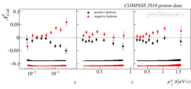
Figure 1.13: The COMPASS Collaboration’s preliminary Collins single spin asymmetry results in semi-inclusive deep-inelastic scattering on a transversely polarized proton target  [26].

The observed non-zero Collins asymmetry in SIDIS, which is related to the convolution products of the chiral-odd quark transversity distribution [53] with another chiral-odd object the “Collins Fragmentation Function”, strongly indicated that both the quark transversity as well as the quark to hadron Collins fragmentation functions are non-vanishing. The similar amplitudes and the opposite signs of positive-hadron SSA relative to that of the negative hadron indicated that the the up-quark transversity is opposite to that of down-quark, but similar in amplitudes, and the “unfavored” Collins fragmentation function is opposite in sign to that of the “favored” one, perhaps with an even larger amplitude. Independently, effects of non-zero Collins fragmentation function have been observed by the BELLE Collaboration  [3] in $e^{+}e^{-}$ annihilation and the quark to hadron Collins fragmentation function have been first extracted from these data [18].

The existence of non-zero Collins fragmentation function allows the extraction of the quark transversity distributions inside the nucleon. Transversity or $\delta q_{f}(x)$, is one of the three leading order quark distributions which survive the integration of quark transverse momentum. They are: quark momentum distribution $f_{q}(x)$, helicity distribution $\Delta f_{q}(x)$ and transversity distribution $\delta q_{f}(x)$. Quark transversity is a measure of the quark’s spin-alignment along the nucleon’s transverse spin direction, and it is different from that of helicity distribution since operations of rotations and boosts do not commute. The $0^{th}$-moment of transversity, $\sum_{f}\int_{0}^{1}\delta q_{f}(x)dx$, yields nucleon’s tensor-charge as one of the fundamental properties of the nucleon just like its charge and magnetic moment. Transversity requires a helicity change of 1-unit between the initial and the final state of the parton such that gluons, which have spin-1, are not allowed to have transversity. Therefore, quark transversity distribution is sensitive only to the valence quark spin structure, and its $Q^{2}$ evolution follows that of non-singlet densities which do not couple with any gluon related quantities, a completely different behavior compared to that of the longitudinal spin structure. These attributes provide an important test of our understanding of the anti-quark and gluon longitudinal spin structure functions, especially with regard to relativistic effects. Quark transversity distributions and quark spin-dependent Collins fragmentation functions have been extracted from a QCD global fit [18] of published HERMES proton and COMPASS deuteron SIDIS Collins asymmetries in conjunction with the BELLE $e^{+}e^{-}$ data. The results are shown in Figure 1.14.

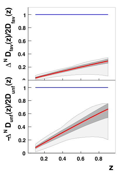
Figure 1.14: The quark transversity (left) distributions, and the Collins fragmentation functions (right) as extracted from SIDIS and $e^{+}e^{-}$ data. In both cases the solid red curve indicates the distributions as determined by the global best fit to the data. The gray bands are an indication of the uncertainty in the extraction. In the left panel, the extracted transversity (solid line) is compared with the helicity distribution (dashed line) at $Q^{2}=2.4$ GeV² and the Soffer positivity bound (blue solid line). In the right panel, the favored and the unfavored Collins fragmentation functions, at $Q^{2}$ = 2.4 GeV²; are compared with the positivity bound and the (wider) uncertainty bands obtained in an earlier fit.

The “Sivers effect”, and the quark Sivers distributions as a completely different mechanism, was thought to be forbidden since early 1990s due to its odd nature under the “naive” time-reversal operation. It was only in 2002 when Brodsky et al. [27] demonstrated that when quark’s transverse motion is considered a left-right biased quark Sivers distribution is not only allowed, it could also be large enough to account for the large observed inclusive hadron SSAs in $p+p$ collisions. Subsequent SIDIS measurements have shown the existence of such non-zero Sivers SSAs, as summarized in Figure1.15 for a comparison of proton Sivers SSA of preliminary COMPASS run-2010 data and the published HERMES data. Clear non-zero Sivers SSA are observed in the positive hadron ($\pi^{+}$ in HERMES) production, while the negative hadron ($\pi^{-}$ in HERMES) SSA are consistent with zero, along with the COMPASS deuteron [15] $\pi^{+}$ and $\pi^{-}$ Sivers SSA, indicating that up-quark and down-quark Sivers distributions are opposite in sign. Such pronounced flavor dependence of the quark Sivers functions were also indicated by a phenomenological fit [19] of the published proton and deuteron Sivers SSA data.

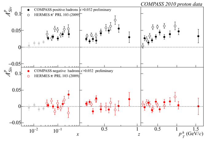
Figure 1.15: The COMPASS Collaboration’s preliminary Sivers single spin asymmetry results in semi-inclusive deep-inelastic scattering on a transversely polarized proton target  [26] compared with that of published HERMES data [12].

Since the Sivers SSA is related to the convolution products of the quark Sivers distributions $f^{\perp}_{1T}$ and the “regular-type” spin-independent quark to hadron fragmentation function, which are reasonably well-known through $e^{+}e^{-}$ annihilation and SIDIS hadron production data, quark Sivers distributions have been extracted through global QCD fits [19] of existing proton and deuteron targets SIDIS data, as shown in Figure 1.16. An illustration of quark 2D density distribution from a Lattice-QCD calculation is also shown, indicating a left-right imbalance of quark density in a transversely polarized nucleon. Sivers function $f^{\perp}_{1T}$ represents a correlation between the nucleon spin and the quark transverse momentum, and it corresponds to the imaginary part of the interference between light-cone wave function components differing by one unit of orbital angular momentum [27]. A nonzero $f_{1T}^{\perp}$ arises due to initial (ISI) and/or final-state interactions (FSI) between the struck parton and the remnant of the polarized nucleon [27]. It was further demonstrated through gauge invariance that the same Sivers function, originates from a gauge link, would lead to SSAs in SIDIS from FSI and in Drell-Yan from ISI but with an opposite sign [31, 28]. This “modified universality” of quark Sivers distribution is an important test of the QCD gauge-link formalism, and the underline assumption of QCD factorization used to calculate these initial/final state colored interactions. A direct test of such a fundamental QCD prediction of Sivers function sign change between SIDIS and Drell-Yan has become a major challenge to spin physics, and it has been designated an DOE/NSAC milestone. Polarized Drell-Yan experiments are currently under preparation at COMPASS and at RHIC IP2, and in the planning stage for both STAR and PHENIX upgrades at RHIC and possibly for a fixed target Drell-Yan experiment at Fermilab. The existence of non-zero quark Sivers distributions is now generally accepted and well defined. Quark Sivers distribution provides an interesting window into the transverse structure of the nucleon, and provides constraints to quark’s orbital angular momentum, although currently only in a model-dependent fashion. Recently, using a lattice-QCD “inspired” assumption that links quark Sivers distribution with quark Generalized Parton Distributions $E$, quark total angular momentum ($J^{q}$) has been quantified [24] for the first time as: $J^{u}=0.266\pm 0.002^{+0.009}_{-0.014}$ and $J^{d}=-0.012\pm 0.003^{+0.024}_{-0.006}$.

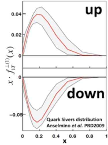
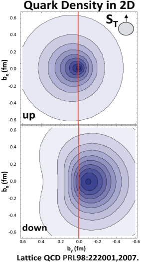
Figure 1.16: The quark Sivers distributions (left plot), as extracted from published proton and deuteron target SIDIS data, for up-quark (top) and down-quark (bottom). The gray bands are an indication of the uncertainty in the extraction. A Lattice-QCD calculation of quark 2-dimensional density distribution in the impact parameter space ($b_{x}$ vs $b_{y}$) for up-quark and down-quark is shown (right plot) with the nucleon polarized in the transverse direction.

Linking the Sivers effect with the twist-3 colinear factorization approach, the twist-3 transverse-spin-dependent quark-gluon correlation function $T_{q,F}(x,x)$ extracted from $p+p$ inclusive SSA data was shown to be directly related to the moments of Sivers functions, thus provide an independent check of our understanding of SSA phenomena in SIDIS and in $p+p$. However, very recent studies by Kang et al. showed that the quark Sivers function moments extracted by these two methods are similar in size, but opposite in sign [44], as shown in Figure 1.17 for the up-quark (left) and the down-quark (right). The solid lines represent twist-3 approach “direct extraction” from $p+p$ inclusive SSA data, while the dashed and dotted lines represent Sivers functions extracted from published SIDIS data assuming two different functional forms. This controversy of Sivers function sign “mismatch” indicates either a serious flaw in our understanding of transverse spin phenomena, or alternatively drastic behaviors [33] of quark Sivers function in high momentum fraction ($x$) or in high transverse momentum ($k_{t}$). Given the facts that the existing SIDIS measurements are limited to $x\leq 0.35$, high precision $p+p$ SSA measurements at very forward rapidity are urgently needed to provide constraints in the high-$x$ region.

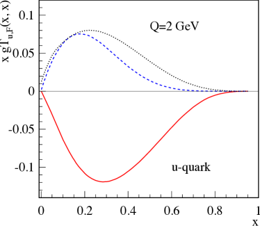
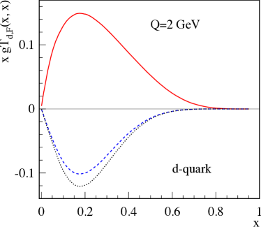
Figure 1.17: The quark-gluon correlation function $gT_{q,F}(x,x)$ as a function of momentum fraction $x$ for $u$-quarks (left) and $d$-quarks (right). The solid lines represent “direct extraction” from $p+p$ inclusive SSA data in the twist-3 approach, while the dashed and dotted lines represent Sivers functions extracted from SIDIS data assuming two different functional forms.

Unlike polarized SIDIS reactions, SSA effects in forward hadron production in transversely polarized $p+p$ collisions are somewhat more complicated to interpret since both the Final State Interactions and the Initial State Interactions exist. From past observations, the single-spin effects in $p+p$ are typically larger than those of SIDIS, thus are much easier for experiments to measure. The main goal of these types of $p+p$ measurements must be to clearly isolate individual effects in SSAs in order to gain a deeper understanding of the fundamental physics. The MPC-EX, along with the Muon Piston Calorimeter (MPC) and the standard PHENIX central and muon-arm detectors, will allow a series of transverse spin measurements to be carried out at PHENIX. Especially, with the capability to reconstruct “jet-like” structures at forward rapidity, two kinds of SSA observables are of particular interest:

1. Hadron azimuthal distribution asymmetry inside a jet ($A_{N}^{h~{}in-jet}$) arises purely from the Collins effect.
   The quark’s transverse spin (transversity) can generate a left-right bias inside a jet. A measurement of $A_{N}^{h~{}in-jet}$ will provide constraints on the product of quark transversity distributions and the Collins fragmentation function Specifically for MPC-EX, the left-right asymmetry of $\pi^{0}$ inside a jet ($A_{N}^{\pi^{0}~{}in-jet}$) is a pure Collins effect. The experimental observable in MPC-EX would be the azimuthal distribution of $\pi^{0}$ yields around the jet axis reconstructed with the MPC-EX, and the azimuthal angle $\phi_{S}$ is between the proton spin direction $\vec{S}_{p}$ and the transverse momentum $\vec{k}_{T}$ of the pion with respect to the jet axis, $\vec{p}_{jet}$ One advantage that such a measurement would have over existing SIDIS measurements would be that the $x$ range measured for the transversity distribution would be substantially higher than that reached in SIDIS, see Figure 1.19. While the next generation SIDIS experiments at JLab-12GeV will extend to high-$x$ region starting in FY-2015, the current SIDIS data do not exceed beyond $x_{Bj}=0.35$,

2. The azimuthal asymmetry of inclusive jet ($A_{N}^{jet}$) arises purely from the Sivers effect.
   The Collins effect does not contribute to $A_{N}^{jet}$ as it averages out in the integration over the azimuthal angle of hadrons inside the jet. A measurement of $A_{N}^{jet}$ will provide information on the product of quark Sivers distributions and the well-known spin-independent fragmentation functions. Predictions of $A_{N}^{jet}$ in the MPC-EX acceptance are at a few $\%$ level with a large range of variations reflecting our lack of knowledge on quark Sivers functions at high-$x$, as shown in Figure 1.18 The measurement of $A_{N}^{jet}$ can be carried out with the MPC-EX by recording the jet yields for the different transverse proton spin orientations and constructing the relative luminosity corrected asymmetries between the yields for the up versus down proton spin orientations.

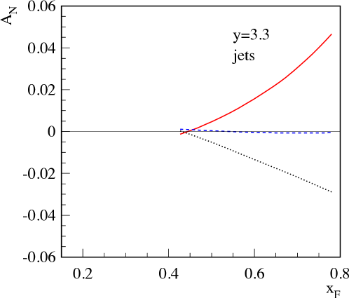
Figure 1.18: The SSAs for inclusive jet production $A_{N}^{jet}$ in $p^{\uparrow}p$ collisions [44] at $\sqrt{S}=200$ GeV, as functions of $x_{F}$ for rapidity $y=3.3$. The solid lines represent “direct extraction” from $p+p$ inclusive SSA data in the twist-3 approach, while the dashed and dotted lines represent Sivers functions extracted from SIDIS data assuming two different functional forms.

Figure 1.19: Bjorken-x distribution in polarized proton for PYTHIA events with a hadron scattered into $3.1<\eta<3.8$ for $x_{F}>0$. A substantial fraction of the data is at $x_{B}>0.35$, where the DIS data ends.

The most critical experimental performance parameters for these type of MPC-EX measurements would include the angular resolution for the direction of the jet axis and the resolution in the hadron momentum fraction $z$. Uncertainties in knowing the jet axis will dilute the amplitude of the azimuthal Collins asymmetry and uncertainties in measuring hadron’s energy fraction ($z=E_{h}/E_{jet}$) will smear the spin analyzing power of the Collins fragmentation function in the stage of data interpretation. The latter of these two is very important, given that the Collins fragmentation function has a strong $z$-dependence, see Figure 1.14.

1.2.2 Other possible SSA measurements with MPC-EX

In addition, not elaborating on the details, we list here other possible SSA measurements with MPC-EX:

1. Prompt photon SSA ($A_{N}^{\gamma}$), which purely arises from the Sivers effect. The expected measurement statistical precision of an MPC-EX measurement (data points from Monte Carlo simulations, see Section 3.5) are shown in Figure 1.20, with theory predictions of prompt photon $A_{N}^{\gamma}$ of Kang et al.[44], which includes contributions from direct and fragmentation photons. Different assumptions for the quark Sivers functions lead to predictions of opposite signs for $A_{N}^{\gamma}$.

2. SSA of back-to-back di-hadrons and back-to-back di-jets.

3. SSA of back-to-back $\gamma$-jet [23] and back-to-back photon-pairs.

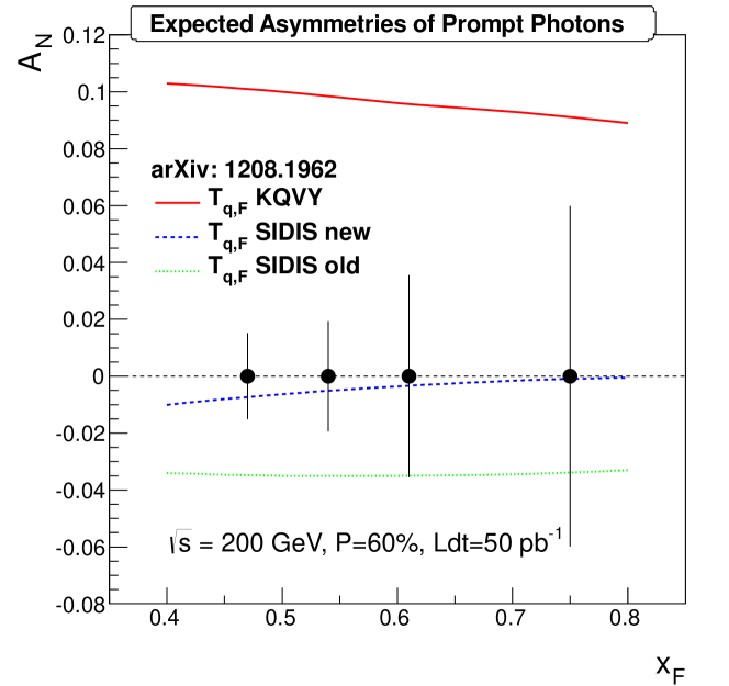
Figure 1.20: The SSAs for prompt photon production $A_{N}^{\gamma}$ in $p^{\uparrow}p$ collisions [44] at $\sqrt{S}=200$ GeV, as functions of $x_{F}$ for rapidity $y=3.5$. The solid lines represent “direct extraction” from $p+p$ inclusive SSA data in the twist-3 approach, while the dashed and dotted lines represent Sivers functions extracted from SIDIS data assuming two different functional forms. The statistical error bars include statistical errors as well as uncertainties introduced by subtraction of background photon SSA originating from meson decays. See Section 3.5 for details.

1.2.3 Measurements Simulated in this Proposal

In order to demonstrate the capabilities of the MPC-EX, we have chosen to simulate a particular observable in detail, namely the correlation of $\pi^{0}$ mesons with the axis of a jet. Such a correlation would yield information about the Collins fragmentation function and transversity within the nucleon. This observable exercises two main features of the MPC-EX: the ability to identify charged tracks, and the ability to reconstruct $\pi^{0}$ mesons at very large momentum. These simulations are described in Section 3.7.

Of course, without full jet reconstruction the MPC-EX cannot measure the full $z$ dependence of the Collins fragmentation function (it can, however, yield measurements in “low-$z$” and “high-$z$” samples by selecting $\pi^{0}$ momentum regions). The main goal of this measurement will be to quantify what fraction of the inclusive $\pi^{0}$ $A_{N}$ results from the Collins fragmentation function and transversity, and by inference, what is the role played by the Sivers effect. In this sense this measurement with the MPC-EX can be considered a “pathfinder” measurement that will point the way to future experiments at RHIC with complete forward spectrometers.

1.2.4 Summary: MPC-EX and the Study of Nucleon’s Transverse Spin Structure

The goal of nucleon spin structure studies is to understand how the nucleon spin is composed of the spin and orbital angular momenta of the quarks and gluons inside the nucleon. With the MPC-EX we will address the following fundamental questions regarding the nucleon’s intrinsic spin structure and the color-interactions that hold together the nucleon’s building blocks:

1. Is a quark’s spin aligned with nucleon spin in the transverse direction ?

2. What is the role of quark’s transverse spin (transversity) during fragmentation ?

3. What is the role of parton’s transverse motion and its correlation with nucleon spin ?

4. What is the role of the color-interactions between a hard-scattering parton and the remnant of the nucleon ?

Specifically, with the new experimental capabilities provided by the MPC-EX, we will make precision measurements that provide clear answers to the following questions:

When a transversely polarized proton produces a very forward jet in a high energy $p+p$ collision, relative to the direction of proton’s spin,

• Would a $\pi^{0}$ particle favor the left side or the right side within the jet (Collins + Transversity)?

• Would the jet itself favor the left side or the right side of the collision (Sivers)?

Chapter 2 The MPC-EX Preshower Detector

2.1 The MPC-EX Detector

The MPC-EX detector system includes both the existing Muon Piston Calorimeters (MPCs) and the proposed extensions which are two, nearly identical, W-Si preshower segments located upstream of the north and south MPCs respectively. This pairing will share the available space inside the PHENIX muon magnet piston pit. Their functionality is largely complementary. The new preshower will

• Improve the quality of measurements of electromagnetic showers in the MPC aperture by reducing the longitudinal leakage of energy,

• Improve the discrimination between electromagnetic and hadronic showers,

• Enable the reconstruction of $\pi^{0}$’s via an effective mass measurement and shower shape analysis to the $p_{T}$ extent allowed by the calorimeter acceptance and RHIC luminosity,

• Measure jet 3-vectors with a precision sufficient to allow a correlation with $pi^{0}$ meson to measure the Collins asymmetry in polarized proton-proton collisions,

• Assist in measuring energies inside jet cone around high-$p_{T}$ lepton candidates for isolation testing.

The current MPC’s[38] (see Fig. 2.1) were installed in 2006 and have already produced a wealth of physics results. With the aim to further extend the physics reach of the existing PHENIX forward spectrometers we have designed extensions (a preshower) to complement the existing MPC’s. By themselves, the MPCs are highly segmented total absorption detectors with a depth of $\sim$18$X_{0}$. The preshower converts photons and will track and measure the energy deposited in the active Si layers by photons and by charged particles. Additionally, the preshower will count and classify hits (as originating from electromagnetic or hadronic showers), measure hit-to-hit separations, and reconstruct effective masses from hit pairs, which can be further used to extract $\pi^{0}$ yields. By measuring the $\pi^{0}$ yields in the same detector, a direct photon extraction can be performed in a self-consistent way, without using extrapolated data with often unknown systematics for background subtraction.

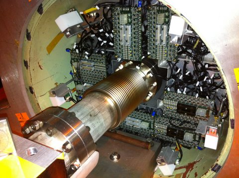
Figure 2.1: A beam view of the North Muon Piston with MPC installed. Signal cables removed.

The MPC-EX’s are located $\sim$210 cm from the nominal collision point north and south of the PHENIX central magnet. The MPC alone is capable of resolving close hits with similar energies down to a separation of the order of 3 cm; this effectively limits the $\pi^{0}$ reconstruction range to momenta below $\sim$15 GeV/$c$. To extend that range towards the $\pi^{0}$ luminosity limit in the forward direction ($\sim$100 GeV) the preshower is designed as a sampling structure of tungsten and active pixelated silicon layers with readout integrated with silicon in the form of micromodules. Silicon provides for versatility of segmentation, while tungsten has a small Molière radius (9.3 mm) so the showers in the preshower are very compact. Tungsten also has an excellent ratio of radiation and absorption lengths, well matching that of PbWO4 (MPC crystals) which is important for electromagnetic energy measurements in the presence of a large hadronic background. The preshower is comprised of eight sampling layers each consisting of 2 mm thick W plate and 3 mm deep readout. The total depth of the preshower ($\sim$$4X_{0}$) is chosen to allow both photons from a $\pi^{0}\rightarrow\gamma\gamma$ decay to convert and be reliably measured in at least two X and two Y sampling layers.

The granularity of the preshower is chosen to match the expected two photon separation in $\pi^{0}$ decays. A $p$ = 100 GeV/$c$ $\pi^{0}$ produced at the nominal collision point will generate two hits in the preshower separated by $\sim$1 cm (compare this to the Molière radius of the detector $\sim$2 cm). To match both the shape of the MPC towers and the minimal two photon separation requirement, the silicon pixels are rectangular in shape and have a transverse size of $\sim$1.8$\times$15 mm². The signal from each pixel is split with a ratio of 1:30 with individual copies sent to two independent SVX4 chips.

The ideal location for this preshower would be flush with the front face of crystals in MPC to minimize large-angle spray fluctuations at the boundary. Unfortunately, this is precluded by the earlier decision to locate the MPC readout (APD’s and signal drivers) upstream of crystals. The actual preshower location on the beam line is also constrained by concerns about additional background to muon tracker station 1 from inside of the Muon Piston pit. This concern will be ultimately decided upon upon completion of integration study of utilities and cable routing which is currently being pursued for the MPC-EX upgrade.

Figure 2.2 shows a three dimensional model of the MPC-EX system installed into the pit of the muon piston. Both components of the system perform calorimetry-style measurements of the energy deposited by charged and neutral particles inside its active volume (crystals in case of MPC and Si in case of preshower). The total sampling depth of the combined detectors (4 $X_{0}$ in the preshower and 18 $X_{0}$ in the MPC) will contribute to the energy measurement.

Figure 2.2: 3D rendering of the Muon Piston Pit with fully installed MPC-EX detector components.

The pit has a diameter of $450$ mm and a depth of $\sim$43 cm. Its opening in front of the MPC is occupied by the sparsely installed MPC signal and power cables (see Fig. 2.1), cooling lines for the MPC, and fixtures supporting beam pipe. A conflict arises between the preshower and MPC monitoring system (distribution boxes), which will be resolved by redesigning MPC cable routing and MPC LED light distribution boxes to illuminate fibers with back-scattered light.

Details of the MPC design can be found in [38]. The mechanical design of the preshower, and its electronics chain and readout, are described in the following sections.

2.2 Detector Design

The physics program described in the first chapter of this proposal requires excellent calorimetry being available very close to beam pipe I both forward directions in PHENIX. The calorimeters must provide good photon energy resolution, reliable hit counting under conditions of extreme occupancy, and two shower resolving power never before implemented in the electromagnetic calorimetry. The Muon Piston Calorimeter (MPC) which covers rapidity range 3.1$<\eta<$4.2 solves this problem only partially. Its transverse momentum range is limited by granularity to $\sim 2.5GeV/c$, it has no resolving power between single photons and $\pi^{0}$ at momenta above $\sim 15GeV/c$ and its resolution is seriously degraded by the presence of sparsly distributed material in front of the detector (beam pipe, BBC, cabling and readout electronics) and radiation damage to crystals. In PHENIX the particles emitted in the very forward direction travel mostly along the direction of magnetic field lines. There are no tracking detectors in the acceptance of the muon piston. High particle multiplicities (especially in the jet events) futher limit the ability of the MPC to address the physics of forward produced direct photons and $\pi^{0}$’s. A meaningful upgrade to the very forward calorimetry required to bring forward jet and direct photon physics within the reach of PHENIX is impossible without major improvement in shower resolving power (a precondition for extaction of the direct photon signal) and single particle tracking in calorimeter (a precondition for jet extraction).

Given the space constraints of the muon piston bore, space is an issue for any new detector component. The space available for the preshower detector is no exception. There is only few cm depth between the tip of muon piston and area already occupied by readout cables and buffer amplifiers of MPC. With this limitation and extreme granularity requirements for detector which must resolve electromagnetic showers as close as 5 mm, a Si based detector becomes the only practical choice for preshower detector. In the past few years our efforts have been primarily directed towards the simulation and R&D of the preshower detector. We opted for a W/Si ionization device so the effect of varying environmental conditions (temperature, humidity) on signal proportionality to energy deposited in readout layers can be either neglected or is easy to monitor with charge injection. In this section we discuss issues such as basic detector geometry and calibration and monitoring schemes.

The depth of the Preshower detector is chosen equal to 4.6$X_{0}$ based upon the following considerations. In the geometry of MPC-EX most electrons (photons) will beging showering in the first one (two) radiation lengths in the preshower . It takes one more radiation length in depth to insure reasonable probability for both photons from high energy $\pi^{0}$ decay to convert and become separately measurable entities in preshower. We add one more $X_{0}$ to the total preshower depth to make sure that both electrons and photons deposit substantial part of their energies in the preshower detector (see Fig. 2.3 which shows longitudinal shower profile [58] for electrons of different energies).

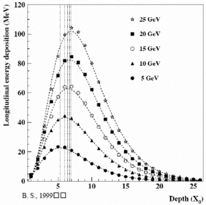
Figure 2.3: Longitudinal energy deposition (dE/dX) for electrons in the energy range 5 to 25 GeV as function of the depth in calorimeter measured in units of $X_{0}$. Lines indicate shower maximum positions at different energies.

Within the first three (four) radiation length of material electrons (photons) deposit on average about 30% of their energy. The choice of depth is nearly optimal in terms of detector sensitivity to electromagnetic vs. hadron variations in the longitudinal shower profile (critical mainly for hadron rejection) and for its resolving power which is based upon its ability to locate individual maxima in the lateral profiles (see Figure 2.4[42]) of electromagnetic showers and to measure shower to shower separation.

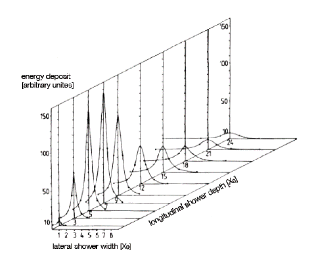
Figure 2.4: Lateral energy deposition for electrons as function of the distance from shower axis in calorimeter measured in units of Molier radius.

The preshower consists of 8 sampling cells each built of  2mm thick W plate and fine position resolution Si readout layer. The Si dtectors are structured into $1.8\times 15mm^{2}$ minipads. The minipad orientation in sequential sampling cells alternates between X and Y to avoid cluster shadowing and allow for separation measurements (see next chapter for details). The over-all granularity of the two-layer XY pair is thus about $2\times 2mm^{2}$. The minipad shaped diodes are implemented on $62\times 62mm^{2}$ silicon wafers $\sim 500\mu$m thick each. Each sensor is laminated with a sensor readout control board (micromodule) which carries 2 readout chips (SVX4) together with a number of passive components and two precision positioned low height microcontact connectors used to connect the micromodule to readout bus on a sensor carrier board. Experience with PC board manufacturing houses shows that given due diligence the positioning of connectors both on a carrier board and SRC can be made to better then $50\mu$m precision resulting in the contribution to uncertainty in hit position of the order of $75\mu$m (compared to $\sim 0.6mm$ intrinsic position resolution of the minipad measurements). The carrier boards are glued to $2mm$ W plates held together by presision bolts penetrating whole depth of the preshower in the areas free of silicon. Alignment between the MPC-EX preshower and MPC will rely on MIP hits in both detectors (measuring edge positions of the shadow of MPC towers in preshower plane).

The preshower is a sampling calorimeter and essentially counts the number of charged particles passing through the silicon. The particles used to calibrate MPC today are mostly pions with momenta of a few GeV. This means they are nearly minimum ionizing, for simplicity we will refer to them as MIPs. We will use the same particles selected in the MPC to reach design goal accuracy of the minipad-to-minipad intercalibration of 5%. After in-situ calibration and measurement of the noise in every minipad , an estimation of the signal to noise ratio for MIP will be made for every individual minipad. The design specification (confirmed in the CERN beam test) for this value is $\sim 10$. We expect on average 32 minipads contributing to shower energy measurements in preshower resulting in the total noise value (pedestal width) of the order of 200 MeV (compare to $\sim 6GeV$ of energy deposited in preshower by a 20 GeV photon).

2.2.1 Sensor Radiation Dose

The MPC-EX preshower will certainly be exposed to high radiation doses. Albedo from the MPC and surrounding PHENIX components, electromagnetic showers, and charged and neutral hadrons from primary collisions are the sources of the radiation in the MPC-EX.

During PHENIX running the muon piston bore is filled with a fairly homogeneous distribution of albedo neutrons with a logarithmic energy spectrum which peaks roughly around 1 MeV (see Section 2.5). We will use D0 estimates for the neutron flux density of $\phi_{n}\ =\ 1.2\times 10^{4}\ cm^{2}s^{-1}$ at a luminosity of $\mathcal{L}\ =\ 10^{32}cm^{-2}s^{-1}$ [36]. Using a conversion factor of $1\ neutron/cm^{2}\ =\ 1.8\times 10^{-9}rad$, the dose from neutrons is given by $\frac{dD_{n}}{dt}\ =\ 2.2\times 10^{-5}rad/s$.

The charged particle flux at rapidity of 4 (corresponding to inner radius of MPC-EX, which is equal to a radius of  7 cm) computed assuming an inelastic cros-section of 50mb and an average multiplicity of 4 per unit of rapidity is $\phi_{\pm}\ \sim 0.5\times 10^{5}\ cm^{-2}s^{-1}$.

Assuming a factor $1/2$ difference between radiation damage due to neutrons and charged particles, taking into account a factor of two for low $p_{T}$ looping tracks, a factor of 10 for particle showering in the calorimeter and an extra factor of 5 for $\pi^{0}$’s, an upper limit for the dose rate related to collision produced particles is given by $\frac{dD_{coll}}{dt}=c_{E}\times\phi_{tot}\times\frac{1}{\rho}\frac{dE}{dx}\ =\sim 7.6\times 10^{-4}$. Adding the rates from neutrons and an upper estimate from collision related particles the total dose rate at $\mathcal{L}\ =\ 10^{32}cm^{-2}s^{-1}$ equals to $\sim 7.8\times 10^{-4}$ rad/s. The total dose rate accumulated at the highest pseudorapidity edge of MPC-EX preshower detector in one year ($10^{7}\ s$) is not expected to exceed 10 krad, or 100 krad for a 10 year running period. This dose rate will result in only minimal radiation damage to silicon sensors. Any related increase in a leakage current is taken care of by decoupling the sensor from the readout chip (see Section 2.4) .

2.3 Mechanical Design

The MPC-EX uses the digital sum of pixel energies measured in a region of interest around a vector pointing from the collision point to a shower found and measured in the MPC. The energy from successive $1.8\times 15$ mm² pixels in the preshower are added to form $\sim$$15\times 15$ mm² towers, with both X and Y pixels allowed to be combined into correlated (partially overlapping) sets of towers. Consequently, defined towers are shower-position dependent and thus could be distinct for different showers, even those which are closely spaced. Their size can be varied depending on the shower width, greatly improving the quality of energy sharing between individual objects. Configured towers are pointing and have energies, positions, hit counts, and object width measured in every sampling layer so both particle identification and particle tracking are simplified and improved. The short (15 mm) length of the pixel makes its energy measurement robust against the adverse effects of occupancy (each layer has $\sim$2500 pixels compared to $\sim$200 crystals in MPC). The advantages of this “configure on the go” approach will be especially important for forward jet measurements which in the case of the MPC-EX system could use both jet definitions based on hit counting in the preshower and the total electromagnetic energy measurements associated with hits in a hybrid preshower/MPC calorimeter.

The radial dimensions and geometry of the preshower were chosen to fit within the envelope defined by the muon piston front face (see Fig. 2.1) coupled the the reorganized MPC signal cables – the last foot of cable length is unjacketed, and the cables will be restrained on the pit wall close to the diver boards. This provides the best match between the preshower and the existing MPC acceptance, resulting in an approximately annular configuration with a central opening of 124$\times$150 mm² to accommodate the beam pipe flanges and support. Note that the actual shape of W absorbers is defined by a 62$\times$62 mm² transverse footprint of the individual Si micromodules.

The preshower is constructed as 2 mm W plates interleaved with readout layers – to allow for micromodule installation the readout layer depth is set to 3.0 mm. G10 carrier boards (0.5 mm thick) are glued to the W plates by conductive tape creating a nearly-perfect Faraday cage for the silicon sensors which are embedded into micromodules pluggable into carrier boards. In designing the micromodules, we decided on a very unconventional design. The sensors are laminated between a 0.4 mm ceramic tile and a 0.4 mm thick sensor readout card (SRC) carrying dual RC network which is used to split the signals and AC decouple silicon diodes from SVX4 input circuitry. The SRC carries two SVX4 chips which combine both analog amplifiers and storage and digitizers and carry two separate grounds (analog and digital). The unconventional part of this design is a presence of digital signals on the traces immediately above the silicon sensors so we went to the extreme to minimize the pickup of digital activity signals on Si. Fortunately calorimetry is forgiving of the additional material in readout layers and a good ground layer between sensor and first layer with traces was sufficient to keep noise level related to digital activity on the board well within SVX4 pedestal width.

We have chosen to use the FNAL-developed SVX4 128 channels pipelined chips as a base for our readout system.

A number of ongoing R&D projects aimed at building similar calorimeters for experiments at a future electron-positron linear collider are considering the option to digitize signals from every pixel in all sampling layers. The proposed solutions are all in their preliminary stages, have a number of constraints (range, power etc), and are expensive. We believe that we have found a unique if not perfect solution to this problem based upon inexpensive and commercially available components which is equally applicable to calorimetry in all kinds of collider experiments. The MPC-EX preshower is the first ever built calorimetry detector with pluggable silicon micromodules and on-detector digital conversion of the analog signals generated by particles passing layers of silicon detectors.

The main design parameters of the MPC-EX preshower can be found in Table 2.1. Details of the readout electronics can be found in Section 2.4.

Table 2.1: MPC-EX Preshower design features. All counts are for a single unit.

Parameter	Value	Comment
Distance from collision vertex	220 cm
Radial coverage	$\sim 18$ cm
Geometrical depth	$\sim 5$ cm
Absorber	W (2mm plates)	$\sim$$0.5\ X_{0}$ or $\sim$$2\%\ L_{abs}$
Readout	Si pixels (1.8$\times$15 mm2)
Sensors	$62\times 62$ mm2	192 ($1.8\times 15$ mm2 minipixels)
Pixel count	24576
SVX4’s	384

2.4 Electronics and Readout

The MPC-EX detector system is composed of eight identical readout layers arranged around the beam pipe in front of the MPC detector. The enclosure diameter is 44 cm. Each layer consists of two identical carrier boards, attached to the tungsten absorber plates. Each carrier board contains 12 plug-in modules with silicon sensors and readout ASICs. The technology for the sensors will be p-on-n detectors with narrow mini-pads 15.0$\times$1.8 mm. The sensors will be orthogonally oriented in alternate layers. To provide a high dynamic range, the signal from each mini-pad is split with ratio 30:1 using a capacitive divider and it is sent to different ASICs.

The electronics unit counts for the MPC-EX, per arm, are:

number of readout planes:	8
number of minipad modules:	192
number of minipads:	24576
number of readout chips:	384
number of carrier boards:	16
number of FEMs:	8

Figure 2.5: Location of the MPC-EX readout electronics in front of the MPC (dimensions are in inches).

The data from the readout ASICs will go to PHENIX DCMs through FEM boards as indicated on Figure 2.6. The FEM will reside on the outer shells of the muon piston magnet and will perform the functions of converting the continuous stream of commands from the control optical fiber into the SVX4 control signals, collecting the data of several SVX4 chains, serializing it and sending it out on data optical fiber to the PHENIX DCMs.

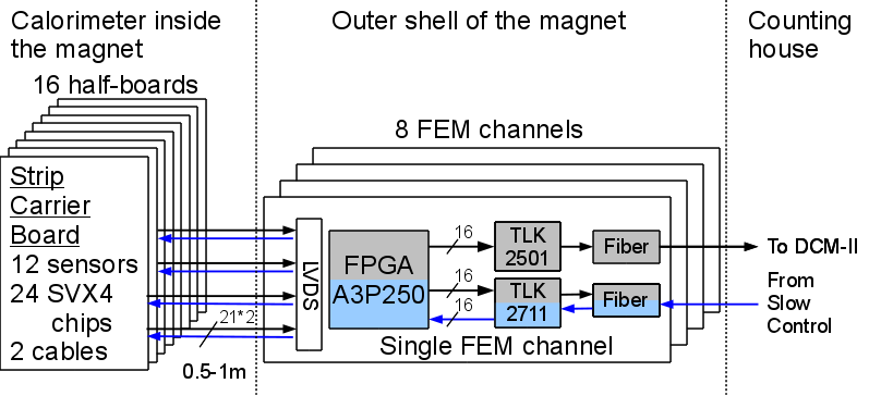
Figure 2.6: Block diagram of the MPC-EX readout electronics components. The blue area - front-end clock domain, the grey area - back-end clock domain.

2.4.1 Strip Readout Module

The design goal of the readout plane is to keep it is as thin as possible to minimize the transversal expansion of the particle shower in the absorber-free areas. The sensor plane consists of two carrier boards (upper and lower) which are conductively attached to the tungsten absorber plates. The carrier board is thin PCB, which has low-profile (0.9 mm thick) connectors where the minipad modules will be plugged in.

The readout card is mounted on top (p+ side) of the sensor, it is wire bonded to the sensor pads at the edge of the sensor using 25$\mu$ Al wires. The positive bias voltage is applied to the backside (n- side) of the sensor using flexible leaf of gold-plated fabric. A thin (0.4 mm) ceramic cover is attached to the backside of the sensor, which provides mechanical rigidity to the assembly.

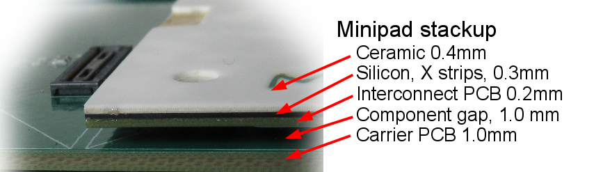
Figure 2.7: Stack-up of the minipad module.

The signals from each of the minipads are routed to two SVX4 ASICs through different decoupling capacitors. The high-gain leg SVX4 is optimized for measuring MIP signals, the low-gain leg SVX4 - for measuring large energy deposition at the center of the shower. The expected energy deposition of the MIP particle in one minipad is 80 KeV, the energy deposition in the central minipad from the 50 GeV electromac shower is expected to be 40 MeV. The ratio between the two legs is 30:1, and is chosen to ensure that the maximal signal in the high-gain leg will, at the same time, be detectable in the low-gain leg.

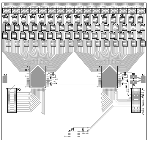
Figure 2.8: Layout and design of the dual-gain SRC. The minipad sensor connections are made at the top of the board, through a set of decoupling capacitor arrays, and then into the SVX4 ASICs.

Each carrier board provides two readout chains with 6 modules per chain. Each chain is connected to an FEM using off-the-shelf low profile flex cable assemblies (JF04 from JAE). All signals in the cable are LVDS, the carrier boards have receivers to convert SVX4 control signals from LVDS to LVCMOS levels. The total thickness of the readout layer is 3.0 mm. The space between adjacent sensors is 0.5 mm. The prototype of the carrier board (see Fig. 2.9) has been designed and tested successfully.

Figure 2.9: Prototype of the carrier board (green) with four installed minipad modules (white).

2.4.2 Dual SVX4 Readout

The dual SVX4 readout has been simulated using LTSpice, the schematics of which is shown in Fig. 2.10.

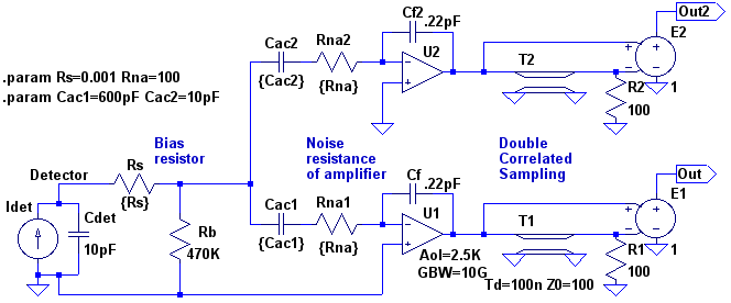
Figure 2.10: SPICE model of the strip readout channel.

The sensor strip is presented as a current source with realistic strip capacitance of 10 pF, the bias resistance is the highest available in a small package. The open gain loop (Aol) of the amplifier is from the specs of the SVX4. The unity gain bandwidth (GBW) was selected to match the published rise time of the SVX4 with the fastest setting. The effective series resistance (Rna) was estimated by matching its contribution to the published ENC versus Cdet dependence. The shaping in the SVX4 is done using a double correlating sampling technique, simulated using an ideal transmission line and a subtractor.

If we assume the infinite open loop gain (Aol) of the operational amplifiers, then the gain of legs Out and Out2 are

G1 = 1/Cf * Cac1/(Cdet+Cac1+Cac2), G2 = 1/Cf * Cac2/(Cdet+Cac1+Cac2).

It can be shown that the S/N at Out is proportional to 1/Cdet and it does not depend on its decoupling capacitor Cac1.

SN1 $\sim$ 1/(Cdet+Cac2), similarly, SN2 $\sim$ 1/(Cdet+Cac1).

To have the SN1 small, we need to choose Cac2 to be as small as possible, but controllable. The reasonable choice is 10 pF. If we select the gain of the low leg, G2 = 1/30 of G1 then the Cac1 should be 300 pF. The simulation, which includes the finite Aol and GBW shows that the G1/G2 = 30 is achieved when Cac2 = 10 pF and Cac1 = 600 pF. The results of the simulation are shown in Figs. 2.11 and 2.12.

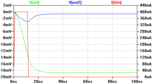
Figure 2.11: Response to one MIP (4.4 fC) charge injection. I(Idet) is the current pulse generated on the detector, V(out) and V(Out2) are the voltage output on the high-gain channel and the low gain channel respectively.

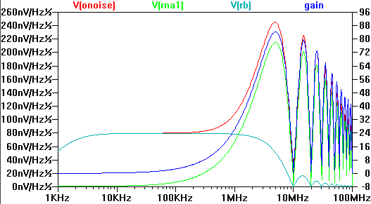
Figure 2.12: Noise analysis. Shown are the gain and spectral densities of the system (V(onoise)) and contributions to it from the preamplifier (V(rna1)) and from the bias resistor (V(rb)).

The signal amplitude of the high-gain leg is 18.68 mV, of the low-gain leg it is 0.64 mV. The main noise contribution above 1 MHz comes from the preamplifier, below 1 MHz - from the bias resistor.

For the high-gain leg, the total RMS noise at Out is 1.17 mV, this corresponds to ENC of 0.28 fC or 1730 electrons. The contribution from Rna1 is 1.04 mV, from Rb is 0.17 mV. If serial resistance of input traces (Rs) is 40 $\Omega$, then the total RMS noise is 1.21 mV. We can conclude that the noise contributions from the bias resistor and from the input traces are not significant.

For the low-gain leg, the total RMS noise at Out2 is 0.76 mV, ENC = 5.2 fC or 32600 electrons, this is slightly larger than 1 MIP but still less than one ADC count.

The saturation level of the pipeline cell of the SVX4 is $\sim$ 100 fC, the saturation level of its preamp is at $\sim$200 fC.

With charge division of 1/30 between two legs we can achieve the following S/N. In the high-gain leg, S/N = 16 for 1 MIP and saturation occurs at 22 MIP or 1.8 MeV deposited energy. In the low-gain leg, saturation occurs at 660 MIP or 32 MeV of deposited energy.

One important feature of this design is that the gain of both legs depends very weakly on the varying detector capacitance.

2.4.3 Front End Module (FEM)

The FEM services up to eight SVX4 chains and serializes them through one fiber link to the PHENIX DCM. The zero suppression of data on SVX4 will be turned off. SVX4 has a unique feature: robust suppression of the common mode noise in real time (RTPS), this will be used to reduce the low frequency noise originating from power supplies and electromagnetic interference. For each trigger every SVX4 generates 129 of 2-byte words. The FPGA in the FEM strips off the channel number byte, selects either the low-gain or high-gain value for output from the two SVX4 and streams the result to the serializer. The input stream of 8 of 16-bit data words @40 MHz is reduced by a factor of four and the resulting stream is serialized with nominal DCM data rate of 1600 Mbps. The first factor of two of reduction is due to the removal of channel bits from the data word, the second factor of two comes from reading out only one of two legs. The leg bits, representing which of the legs was selected for output, are embedded into the output streams (2 bytes of leg bits after 16 ADC bytes).

There are two clock domains in the system as shown on Fig. 2.13: the front-end clock and the back-end clock. The front-end clock, synchronous with the beam crossing, is provided by the PHENIX GTM and it is trasferred to the FEM through the optical link from the Serial Control module. The back-end clock is local to the FEM it synchronizes the data transfer to DCM.

The readout is dead-time free and fully pipelined, the SVX4 can store up to four samples in its input FIFO. Digitization of all channels with 40 MHz front-end clock takes 4.0 $\mu$s. The readout time of one SVX4 at 40 MHz front-end clock is approximately 3.4 $\mu$s. All 8 chains with 12 SVX4s in each can be received into the FEMs FIFO in 45 $\mu$s, the transfer to the DCM can start immediately after the digitization and it will take the same 45 $\mu$s to transfer output data to DCM.

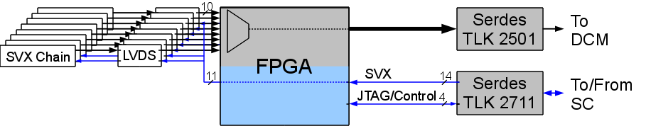
Figure 2.13: Block diagram of FEM board.

The FEM has a very transparent architecture, divided into two, practicaly independent partitions, corresponding to the clock domains - front-end (shown as blue in Fig. 2.13) and back-end (grey). The back-end partition streams out to the data fiber link whatever it receives from the SVX4 chains. The front-end partition simply transfers the SVX4 signals from the Serial Control fiber link to SVX4 chains.

The FEM de-serializes the 16-bit commands coming with the rate of 80 MHz from that link, synchronously with the beam clock. The allocation of parellel bits is shown in Table 2.2.

Four bits of the command word (ADDR*) are used to address the FEMs. Three bits (CTRL*) are reserved for FPGA control: initialization and reset of the beam clock counters are encoded here. Six bits of the command word (SVX*) are translated directly into the signals on SVX chain according to Tables 2.3 and 2.4.

Three bits of the command word and one bit from the SerDes receiver (JTAG*) constitute the JTAG interface. The main purpose of the JTAG interface is the programmatic control of the FPGA in real time, this is implemented using UJTAG macro in the FPGA. The JTAG is also used to re-configure the FPGA firmware. The SerDes for Serial Control connection is the small-footprint TLK2711 working at 1.6 Gbps, the SerDes for DCM connection is TLK2501.

Table 2.2: Serial Control bit assignment.

Bit	In	Out
1	In[0]	ADDR_CS[0]
2	In[1]	ADDR_CS[1]
3	In[2]	ADDR_CS[2]
4	In[3]	ADDR_CS[3]
5	In[4]	CTRL_Cmd[0]
6	In[5]	CTRL_Cmd[1]
7	In[6]	CTRL_Cmd[2]
8	In[7]	SVX_FEClk
9	In[8]	SVX_Trig[0]
10	In[9]	SVX_Trig[1]
11	In[10]	SVX_Mode[0]
12	In[11]	SVX_Mode[1]
13	In[12]	SVX_Readout
14	In[13]	JTAG_TMS
15	In[14]	JTAG_TCK
16	JTAG_TDO	JTAG_TDI

Table 2.3: Trigger[1:0] encoding

Code	Action	SVX signals
0	no action
1	Trigger	L1A
2	Abort gap	PARst,PRD2
3	Calibration	CalSR

Table 2.4: Mode[1:0] encoding

Code	Action	SVX signals
0	Configuration	FEMode=0
1	Reserved
2	Acquire	FEMode=1, BEMode=0
3	Acquire&Digitization	FEMode=1, BEMode=1

The power consumption required for one arm is approximately 110 W for all 16 carrier boards and 20 W for the 4 FEMs. The details are shown in Table 2.5.

Table 2.5: Power budget for the FEM and carrier boards.

Board	Line	Voltage	Current	Wattage
Carrier Board	AVDD SVX4	2.5V	2.0A	5W
	DVDD SVX4	2.5V	0.5A	1.3W
	DVDD LVDS	2.5V	0.2A	0.5W
Total				6.75W
FEM	DVDD LVDS	2.5V	1.0A	3.8W
	FPGA Core	1.5V	0.6A	0.9W
	FPGA IO	2.5V	0.2A	0.4W
Total				5.1W

The JF04 cable assembly between the FEM and the carrier board carries 21 LVDS pairs and also a ground plane and 9 extra lines – which can be used to provide power to the carrier board. The powering of the carrier boards from the FEMs through the signal cable simplifies the cable routing in the tight area of the muon piston magnet but it may have an impact on the noise figure of the system and should be tested before the final installation in PHENIX.

The current FEM channel design, serving 4 of the SVX4 chains has been successfully implemented on a Virtex-II XILINX FPGA. The full design for 8 chains will be implemented using more radiation hard A3P1000 ACTEL FPGA.

2.4.4 Serial Control

The Serial Control module is responsible for the following:

distributes the front-end clock from the PHENIX GTM to the FEMs,

generates trigger and SVX4 control signals from mode bits of the PHENIX GTM,

provides run control of the FEMs,

provides configuration of the SVX4 chains,

provides configuration for FPGA in FEMs,

monitors the status of the FEMs

All this information is sent to and from FEMs through the optical fibers. The Serial Control FPGA contains several serial transceivers, one transceiver is used to emulate the fixed-latency GLINK protocol of the GTM, the rest are used to connect to FEMs. Communication with the external world over ethernet is provided by a micro-processor unit Digi ConnectMe 9210 from Digi International, which is embedded into the modular ethernet jack.

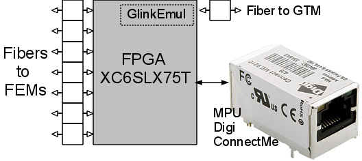
Figure 2.14: Block diagram of the Serial Control module.

The communication protocol between MPU and FPGA as well as graphical user interface to the Serial Control have been developed and tested on the FEM prototype.

2.4.5 Radiation Environment and Component Selection

The FPGA used in FEM is FLASH-based, the same FPGA family as used in PHENIX SVTX and FVTX subsystems. It is immune to configuration loss due to neutron irradiation (firm errors).

FLASH memories exhibit dissipation of the charge on the floating gate after 20kRad of integrated dose. The dissipation is not permanent damage and is remediated by reprogramming the device. Flash memories also displayed SEE problems when programmed during radiation exposure that included gate punch-through, a destructive effect. These types of SEEs are avoided by not programming the FLASH under radiation exposure conditions, namely during machine operation. The Single Event Upsets (SEU) will be mitigated using Triple Modular Redunduncy (TMR) technique.

2.5 Impact of the MPC-EX on Existing PHENIX Detector Systems

2.5.1 Neutrons

The addition of dense material in the muon piston hole can potentially have severe effects on other detector subsystems. The hole or cut-out in the muon piston was originally motivated by neutron studies in order to move the origin of spallation products far back into the iron yoke. This way, the yoke itself serves as an effective shielding of the active detector components of the muon tracker stations gainst secondary particles from the spallation process. Furthermore, the MPC is now located inside the piston hole. Several radiation legths of material in front of the detector can cause increased radiation damage in the PbWO₄ crystals and large fake signals in the read-out electronics.

We study the effect of additional tungsten layers in the muon piston hole with a GEANT4 based Monte-Carlo simulation. This simulation was developed especially for the investigation of thermal neutrons from spallation processes in the context of a new steel absorber in the PHENIX muon arms. The geometry includes a full representation of the south arm tracker stations with a slighly reduced acceptance compared to the north hemisphere ($12^{\deg}<\theta<30^{\deg}$). The simulation uses primary particles from PYTHIA generated events in a forward direction of $\theta<45^{\deg}$. Consequently, the central magnet iron yoke with both copper coils is included in the setup together with the copper nose cone and the copper flower pot with lead end-caps. Also, more importantly for the current studies, both the BBC quartz and the MPC crystals are represented by a cylindrical mock-up geometry. All materials are constructed with the complete isotope composition on top of the chemical structure. The correct isotope mix is important for the thermalization process of neutrons when they scatter elastically from nuclei. It also can change the neutron absorption cross section significantly over a wide range of energies. We use the QGSP_BERT_HP package in GEANT4 for interaction and processes with its default settings instead of tuning all particle and material cut-offs manually. This package has been tuned for the thermalization of neutrons and includes electromagnetic and hadronic interactions down to a few eV with neutron capture modelled from world data. While the total flux of particles from spallation may be off by a factor of two or so, we currently only use the simulation to compare changes in the setup. The absolute normalization can be infered from measured data in the years 2010 and 2011.

For previous studies, we focused on the three muon tracker stations where a big pulse background has been observed with a strong timely correlation to proton proton collisions (heavy ion collisions, respectively). This background was assumed to be from thermal neutron capture and subsequent gamma emmission in material close to the active gas volume of the muon tracker stations. Although the quantitative time structure of the thermal neutrons could not be reproduced in the simulation in detail, it was shown that the gamma emmission was indeed consistent with the measurement. Medium and low energy neutrons are typically behaving very much like a gas in the muon tracker volume. Neutrons from the main spallation source in the back part of the muon piston hole can easily reach into the muon trackers, either by diffusion through the iron piston or by expanding and moving around the hole opening. Thermalization typically happens after the neutrons have already left the constrained volume of the piston hole. Those neutrons can pass through the active detector parts many times before being captured. In summary, differences between the neutron exposure of the three muon tracker layers are mainly scaling with the general geometry, i.e. distance and size. In the following we use the first station (MuTr1 in Figures 2.15 and 2.16) as a (worst case) proxy for the whole muon tracker volume.

For the purposes of thermal neutrons in the muon trackers, the MPC has previously been a minor obstruction in the muon piston hole that shifts the main origin of spallation a little towards the opening (upstream). In order to also estimate the impact of the new pre-shower on the MPC, we include an additional active detector in place of the APDs and the pre-amplifiers in front of the PbWO₄ crystals.

The neutron flux results of the simulation are presented in Figure 2.15. We choose two energy ranges to illustrate the behavior of the neutron spectra depending on the location of the detector. The slow neutrons behave very gas-like, the steep incline towards the lower end of the spectrum here ($E_{neutron}<0.4$ eV) are thermal neutrons. The fast neutrons are not very different from high energetic neutrons in that their tracks are rather straight as compared to the gas-like thermal neutrons. The shape of the spectrum looks very ragged, but a general fall-off with energy can be seen that is almost exponential all the way up to a few GeV. Therefore, the fast neutrons can be also be taken as a good proxy of variations in the total neutron flux where most of the energy is contained which is the important parameter for the radiation damage in the MPC.

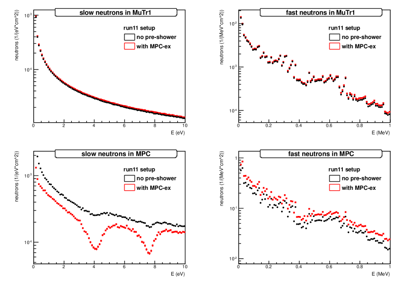
Figure 2.15: Slow (left) and fast (right) neutron fluxes in the location of muon tracker station 1 (top) and the read-out of the existing MPC (bottom).

As expected, the slow neutrons in the muon tracker stations (top left in Figure 2.15 are very little affected by the inclusion of additional tungsten layers in the muon piston hole. Although the main spallation happens in the tungsten now, most of those high energetic neutrons leave the piston hole before they thermalize. Thermalization times are on the order of 30 $\mu$s and it happens either the muon piston steel or (more likely) in hydrogen rich materials in the muon tracker volume (plastic in the electronics read-out). We like to point out that the piston hole still serves its purpose in that there is ample free space both in front and behind the pre-shower tungsten layers. If the whole volume was filled with heavy material, the neutron flux in the muon tracker stations would likely be significantly increased from neutrons emerging from the front of that material. As a side note, the slow neutrons in the MPC are actually reduced by the tungsten in front of it, see bottom left of Figure 2.15. We see two very broad absorption resonances which have been confirmed from other data, too (and a hint of them is already observed from the tunsten content in the crystals of the MPC themselves). Again, this is evidence that the thermalization takes place outside of the piston hole; the neutrons are then captured in the tungsten before they can reach the MPC.

The spectra do include statistical errors, so the variations we see in the fast neutron spectra are real, right side of Figure  2.15. They do correspond to different absorption resonances in the material mix in the whole detector setup. Generally, the spectra in the muon tracker and the MPC show the same distinct features, e.g. the two rising spikes at $E_{neutron}\approx 0.3$ MeV and the flat area around 0.5 MeV. Minor variations are expected in the proximity of different elements. In summary, the inclusion of additional tungsten in the piston hole leads to a slight increase in the fast neutron flux in the muon tracker volume. This probably is due to secondary spallation from an upstream shifted primary spallation. Not surprisingly, the fast neutron flux in the MPC is increased significantly.

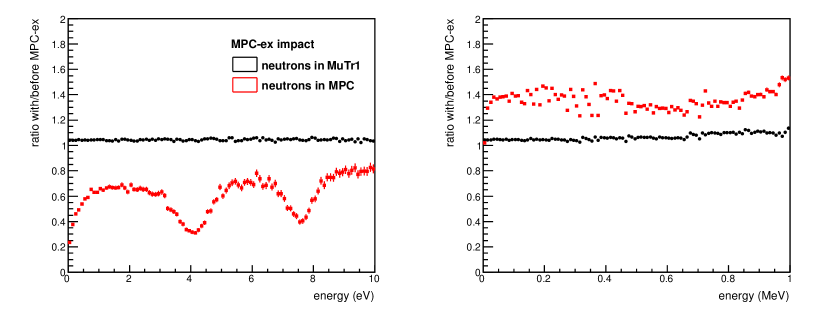
Figure 2.16: Impact of the tungsten layers of the pre-shower on the slow and fast neutron flux on the muon tracker station 1 and the MPC read-out (APDs and pre-amps).

Figure 2.16 is a quantitative summary of the effects of additional tungsten layers as part of a pre-shower in front of the MPC. For the moun tracker, the thermal neutrons are the main concern because they likely lead to the big pulse background that has been observed in real data. From the simluations we conclude, that we do not an increase in this background by more than 5%. Both the fast neutrons and the total neutron flux can lead to a significant performance reduction of the MPC. We estimate this effect to be on the order of 30-40%. This increase is not negligible, but it is on the order of what we expect from a high luminosity and high energy environment, $\sqrt{s}=500$ GeV instead of 200 GeV.

2.5.2 Effect of the MPC-EX on MPC APDs

The MPC is read out with avalanche photodiodes (Hamamatsu model S8664-55) mounted on the front face of the MPC crystals. The original motivation for this location for the APD’s (as opposed to the rear of the crystals) was in part to avoid the effect of leakage of charged particles from the back of the MPC crystals into the APD’s. Charged particles depositing ionization in the silicon of the APD prior to the avalanche region will create a signal that will be amplified by the same gain as the light from the crystals. When the MPC-EX is installed in front of the MPC the electromagnetic showers will be partially developed at the location of the MPC APD’s and they will see a significant charged particle flux. This could potentially affect the energy calibration and resolution of the MPC.

In order to measure this effect we first estimate the number of charged particles at the location of the APD’s for a sample of photon showers in the PISA simulation with energies between 5-100GeV. The number of charged particles at the location of the APD’s is estimated by summing the ionization energy in the last layer of the the MPC-EX silicon and dividing by the energy deposited by a minimum ionizing particle (MIP) in a 300$\mu$m thickness of Si ($\sim$ 116 keV). This is almost certainly an over-estimate, as it does not account for the fact that some shower particles will be very low energy and will stop in the silicon. For low-energy electromagnetic showers (5-10 GeV) the average number of MIPS at the longitudinal location of the APD’s is 6 MIPs/GeV of incident energy. At higher energy this average drops a bit, down to 5.4 MIPs/GeV at shower energies of 35 GeV.

The MPC APD’s cover a smaller area than the MPC crystals, 25$mm^{2}$ compared to 400$mm^{2}$. Typically the central tower in the MPC contains $\sim$40% of the shower energy. The CMS collaboration has studied the effect of minimum ionizing particles on similar Hamamatsu APD’s in a test beam by exposing a test setup to high momentum muons [45]. As expected, the effect depends on the size of the depleted region in front of the avalanche region. For an APD gain approximately equal to 50 the equivalent response to a MIP in the APD’s was between 145 and 520MeV, depending on the terminal capacitance of the Hamamatsu APD. The MPC APD’s are operated at a gain of 25, which means that a single MIP in the MPC APD’s should contribute an equivalent signal between 73 and 260MeV.

Based on the above we can estimate the additional energy due to the flux of charged particles through the MPC APD’s as:

$$E_{charged} = 6MIPs/GeV\times 0.7\times(25mm^{2}/400mm^{2})\times(145-520MeV/MIP)$$

$$= 38-136MeV/GeV$$

which is equivalent to between 4-14% additional energy measured by the APD’s. This can be easily accounted for in the calibration of the energy response of the combined MPC-EX and MPC detectors and should not significantly influence the energy resolution. Fluctuations due to the shower development in the MPC-EX be accounted for by using the MPC-EX track location relative to the APD’s and the depth of the starting point of the shower, as well as an estimate of the number of MIPs exiting the MPC-EX shower from the energy deposition in the last layer. Therefore, we conclude that it while the effect of the MPC-EX will need to be included in calibrating the MPC, it will not be necessary to redesign the MPC detector to move the APDs.

The MPC-EX collaboration is investigating the possibility of testing the MPC APD response in a test beam at FNAL in late 2012 in order to verify the CMS measurements.

Chapter 3 Simulations and Physics Observables

To demonstrate the physics capabilities of the MPC-EX we have performed extensive simulations of two key physics observables. The first, the measurement of direct photons in d+Au collisons, is extremely challenging experimentally but offers a sensitive measurement of the suppression of gluons in nuclei at small-x. The second, a measurement of the azimuthal asymmetry of hadrons within jets in polarized proton-proton collisions, can elucidate the origin of the single-spin asymmetries observed at large $x_{F}$ in hadron collisions.

We begin by first describing the reconstruction method and performance in the MPC-EX in identifying $\pi^{0}$ mesons, photons and charged hadrons. This is followed by specific descriptions of the measurement for direct photons and $\pi^{0}$ correlations in jets. Our strategy is to use a full simulation of the PHENIX detector including the MPC-EX to simulate the observables as completely as possible. From these simulations we extract the expected experimental sensitivity we for given sample of integrated luminosity.

3.1 Reconstruction of electromagnetic showers.

3.1.1 Overview of Section

The method used for reconstructing electromagnetic showers in the MPC-EX is detailed in this section. Specifically, a discussion of the reconstruction in general terms is given, with little consideration of the source of the e-m shower (i.e. $\gamma$ or $\pi^{0}$).

The detector, as described previously, uses eight layers of silicon strips to determine a track vector and its energy from localized clusters of hits. The overall aim of this section is to describe how the clusters are formed in the MPC-EX, how the energy of the preshower is determined, and finally how the preshower is connected to the existing MPC cluster reconstruction. This section does not discuss the cluster-finding algorithms employed in the MPC reconstruction, but focuses solely on the preshower.

3.1.2 Preshower Cluster Reconstruction

The methodology used for the cluster-finding in the preshower is quite simple. Tracks in the MPC-EX preshower are determined in “Hough” space for ease of matching. In Hough tracking, the coordinates of the track are converted into “Hough” parameters. For the case of neutral particles, or those which do not deviate from a straight line trajectory, the Hough parameters are the slope ($x$/$z$ or $y$/$z$) and intercept. This is far more convenient as these parameters are the same for each layer of silicon in the preshower and the same for the MPC itself. By contrast, tracking or track matching with Cartesian coordinates would be more difficult as the $x$ and $y$ positions change with the $z$ position of the layer. When many points of reference are available, localized slopes and intercepts between each pair can be created allowing both the slope and intercept to be used for matching. In our case, the number of layers is small, so the Hough parameters are formed using the intercept (vertex position) and each point. Thus, only the slope parameter is used in the track finding in the MPC-EX and later track matching with the MPC.

Towers of minipads are formed in Hough space from the sum of minipad energies in successive layers. The $x$ and $y$ oriented minipads are independently summed. Each tower consists of four minipads (one per layer) which have the same $x$ and $y$ Hough parameters, but different $z$. Figure 3.1 shows hits in layers 0&1 (for $x$ and $y$ oriented layers respectively), 2&3, 4&5, and 6&7 (left to right). The colors represent the amount of energy deposited in the minipads: purple/blue are low energy hits, yellow/red are high energy hits. The summed energies are shown in Figure 3.2 as towers. The two views show different perspectives of the same event.

Next, a search for all possible peaks of energy in the minipad towers performed using the tower energies (see Figure 3.3 for a cartoon of this). A search window of eight towers is defined. Within the search window, the tower with the highest energy is considered to be a candidate for forming preshower track; only one peak per window is allowed. In the next step, the search window is shifted by one tower, i.e. seven original towers, plus one new one. A new peak is sought. If the peak is the same as a previous peak, it is not added to the list of candidates. The whole detector is scanned to find all possible peaks. The top row of Figure 3.3 shows one sensor (32$\times$4 minipads) being searched for peaks. The bottom row shows more details of the corresponding search windows, with energy deposits illustrating the found peaks. Purple/blue colors represent small energy deposits in the tower, whilst yellow/red colors represent large energy deposits in that region. In the first column, the peak is found in the third tower. In the second search window, the same peak is found. In this example, a second “peak” is not added to the candidate list until the third search window is reached. (That peak would have been defined in the fourth search window trial, but this is not shown in the cartoon.)

Figure 3.1: Hits in successive layers 0&1, 2&3, 4&5, and 6&7 ((left to right). Colors represent the energy deposited in a particular minipad – purple/blue are low energy, yellow/red are higher energies.

Figure 3.2: Two views of the energy deposited in “towers” from the same event in Figure 3.1. Colors represent the energy deposited in a particular minipad – purple/blue are low energy, yellow/red are higher energies.

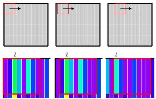
Figure 3.3: Cartoon showing the reconstruction procedure. The upper panels depict the full (32$\times$4) sensor, the lower are zoomed in on the region in question for that particular step. The colors in the lower panel show the energy recorded in a particular minipad (purple/blue are low energies, yellow/red are high energy). The leftmost column shows the starting point of the reconstruction, the center shows the next step, i.e. moved over one minipad. The rightmost column shows a few steps later. The red outline shows the current search window. A single peak is found in each window corresponding to the highest energy deposited in a single minipad.

For each preshower track candidate, the track energy and energy-weighted track-vector is calculated as the sum of energy deposited in a region that is 48 strips wide in the “short” dimensions of the strips, and three strips wide in the long dimension. This yields an average position over many minipads, rather than the position of the highest-energy hit. Figure 3.4 shows a comparison of the Hough space resolution between the highest energy minipad and the energy-weighted average. The latter has a superior resolution. A new energy (summed over the central and surrounding towers) and an improved energy-weighted track-vector is recalculated for added precision.

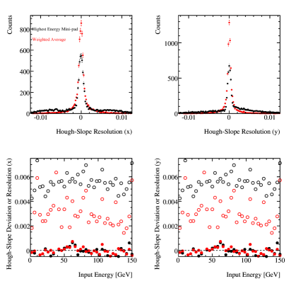
Figure 3.4: Comparison between the resolution determined from the highest energy minipad (trial peak position - black symbols) and that from the energy-weighted average (red) for single input $\gamma$s. The top panels show the the difference between the reconstructed and true Hough slope for the $x$- and $y$-directions, left and right figures respectively. The lower panels show the mean deviation (solid symbols) and resolution (open) as a function of true energy.

3.1.3 MPC Cluster Pointing Resolution

The MPC has an intrinsic limitation in its pointing resolution due its tower size. Figure 3.5 shows the $\eta$ (left panel) and $\phi$ (right) resolution for MPC Clusters, versus the true energy of the particle. A resolution of $\Delta\phi(\eta)$$<$0.04 is observed for high momentum track (i.e. $E_{Input}$$>$30 GeV). Tracks at lower momenta have a worse resolution owing to the diminished energy available for showering and (for $\pi^{0}$s) the deflection of decay $\gamma$s from the original direction.

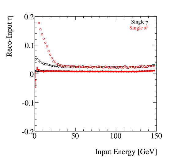
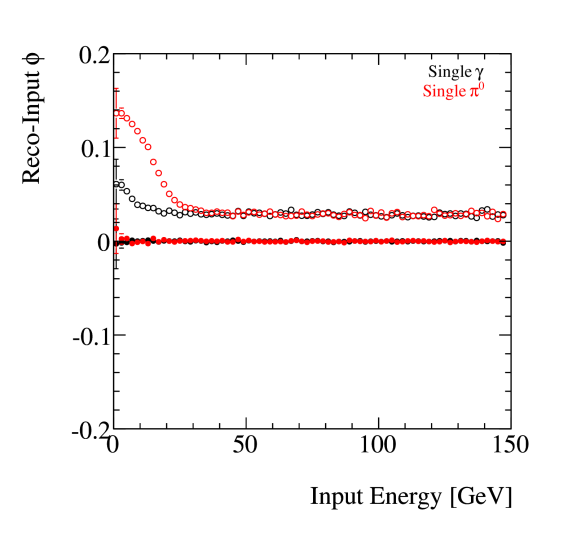
Figure 3.5: Pointing resolution of the MPC for single-$\gamma$ (black) and single-$\pi^{0}$s (red) versus the true energy of the particle. The left (right) panel shows the $\eta$ ($\phi$) resolution (open symbols) and offset (closed). The deviation between $\pi^{0}$s and $\gamma$s observed at low energies is due to two distinct MPC clusters being found.

In terms of the resolution in Hough space, Figure 3.6 shows various prospective Hough slope differences between the MPC and the pre-shower, representing a possible quality control cut (see below). The resolution of the MPC is good enough such that a very tight cut on this parameter can be used, reducing contamination from additional particles.

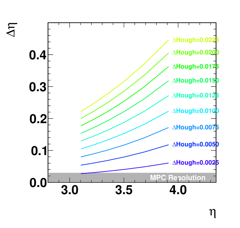
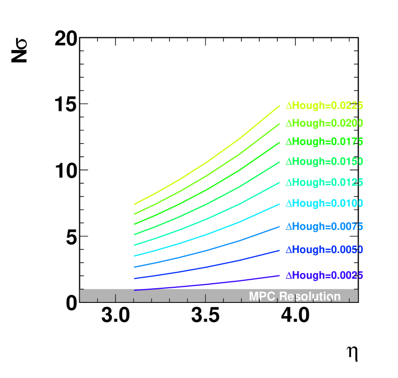
Figure 3.6: Hough slope difference cut compared to the pointing resolution of the MPC. The left panel shows the absolute $\Delta\eta$ for a prospective difference in Hough slope between the MPC and the pre-shower. The right panel shows the same data, but divided by the approximate resolution of the MPC (0.03). Colored lines represent the limit of difference between the MPC and the pre-shower. The grey box shows the approximate MPC resolution.

3.1.4 Track Matching

The cluster-finding procedure of the MPC is completely independent of the one used in the preshower. To join the two systems, the track-vector found for each preshower track candidate is compared to each cluster found in the MPC. In Hough space, the closest matched MPC cluster is assigned to a preshower candidate. As this allows multiple preshower candidates to be associated to a single MPC cluster. A scan through all candidates with the same MPC cluster is made to determine which preshower candidate is the closest. Figure 3.7 shows the difference in Hough slope found between the closest MPC cluster to a given MPC-EX track candidate. The right panel shows the energy dependence of the mean of $\Delta(Hough)$ distribution (the distance in the 2-dimensional Hough space). One reason for multiple tracks is fluctuations in the showering process which can form a spur of hits in multiple layers that happen to line-up in Hough-space. Multiple tracks can also be formed from the decay of particles, for example $\pi^{0}\rightarrow\gamma\gamma$. These are treated in a second peak-finding algorithm.

For illustration, Figure 3.8 shows the number of MPC-EX track candidates found per MPC cluster found for single-$\gamma$s (left) and single-$\pi^{0}$s (right). Once the closest MPC-EX track to an MPC cluster is determined, a clustering algorithm is used to recombine all tracks within a radius of 0.0175 in Hough space. This track is then associated with the MPC cluster. The constituent tracks of the cluster are eliminated from the track list.

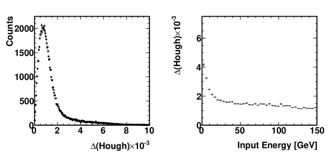
Figure 3.7: The left panel shows the $\Delta(Hough)$ distribution in a single-$\gamma$ simulation; the right panel shows the dependence on the true energy.

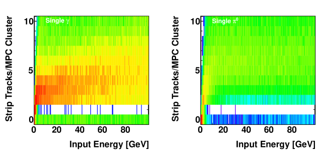
Figure 3.8: Number of minipad-tracks per MPC cluster. The left panel shows a simulation of single-$\gamma$s, the right shows single-$\pi^{0}$s. The color scale is logarithmic.

3.1.5 Energy Recalibration

When working with real data, the whole MPC-EX detector will be calibrated as a single unit. This can be performed in the low-energy region iteratively using pairs of clusters to form an invariant mass. A comparison between the known mass of the $\pi^{0}$ and the $\eta$-meson will facilitate the calibration. For high-energy clusters, the single-track approach (discussed in Section 3.2) can be used to verify (or fine-tune) the calibration. For the purposes of this document, a full calibration procedure has not been developed. Rather, a re-calibration of clusters produced using the existing infrastructure is performed. This procedure is necessary as the current calibration assumes there is no impediment to photons prior to the MPC, whereas the MPC-EX represents approximately four electromagnetic radiation lengths.

The reconstructed energy is formed independently from the silicon preshower and the MPC crystals. Figure 3.9 (left panel) shows the amount of energy typically deposited in each section as a function of the true energy. Less than 20% of the total true energy is reconstructed in the preshower. To estimate the total energy, one needs to recalibrate the energy reconstructed in the MPC. Here, we simply apply an additional calibration to the reconstructed energy in the MPC from the existing reconstruction algorithms.

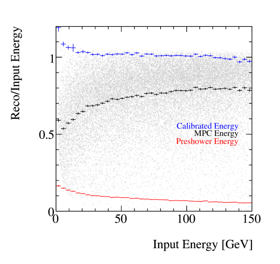
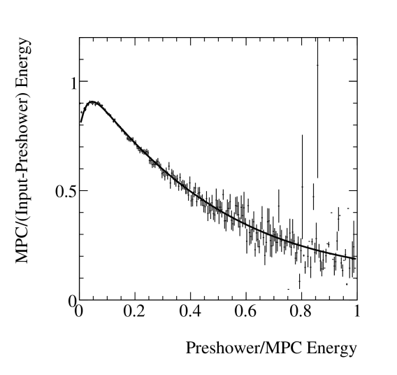
Figure 3.9: The left panel shows the energy deposition in the preshower (red) and MPC (black profile, grey symbols). The blue histogram represents the calibrated data. Most energy is deposited in the MPC, with a diminishing amount in the preshower for larger true energies. The right panel shows the calibration method used, see text for details.

The calibration itself is a two-pass procedure. The relevant scaling variable for the first pass is the ratio of the preshower to the MPC energy, $fRat$. The calibration is made from a sample of single $\gamma$s at various energies. The measured MPC energy is divided by the known true energy of the $\gamma$ minus the measured energy from the preshower. This difference then represents the amount of energy which needs to be reconstructed in the MPC. Figure 3.9 (right panel) shows this ratio as a function of $fRat$. The distribution is fit with a ninth order polynomial in the region 0.1$<fRat<$1. The total energy $E_{TOT}$ is calculated by summing the MPC-EX energy and the corrected MPC energy. The total energy is then subject to a second-order scaling correction based on the reconstructed total energy. The parameters used in the first and second-pass calibrations are in Table 3.1. For cases when the preshower energy exceeds that of the MPC, the energy calibration is fixed to a constant value (corresponding to $fRat=1$), due to statistical limitations in the calibration of the simulation data. The final calibration can be seen in the left panel of Figure 3.9 (blue symbols). The reconstructed energy in the region of interest ($E>$20 GeV) is in good agreement with the true energy.

Table 3.1: Parameters for first- and second-pass energy calibration.

Function	Parameter	Value
	Number
First Pass (MPC Energy), Polynomial ($fRat$)	0	1.00492
	1	0.571689
	2	-14.6354
	3	371.281
	4	-2608.27
	5	8990.66
	6	-1.67062 $\times 10^{4}$
	7	1.6094 $\times 10^{4}$
	8	-6327.06
Second Pass (Total Energy), Polynomial ($E_{TOT}$)	0	1.04137
	1	-0.009866
	2	0.000506
	3	-1.2361 $\times 10^{-5}$
	4	1.595451 $\times 10^{-7}$
	5	1.02758 $\times 10^{-8}$
	6	2.5889 $\times 10^{-12}$

The energy resolution of the combined MPC-EX + MPC after calibration of the simulations is shown in Figure 3.10. In the energy range of interest for the direct photon ($E>$20 GeV) the energy resolution is below 6%. The large constant term in the fit to the resolution is likely a result of the imperfect method used to combine the MPC-EX and MPC detectors, and will certainly be improved in real data when a combined reconstruction procedure is used. As a comparison, the MPC alone achieved and energy resolution of roughly $14\%/\sqrt{E}$ in a test beam.

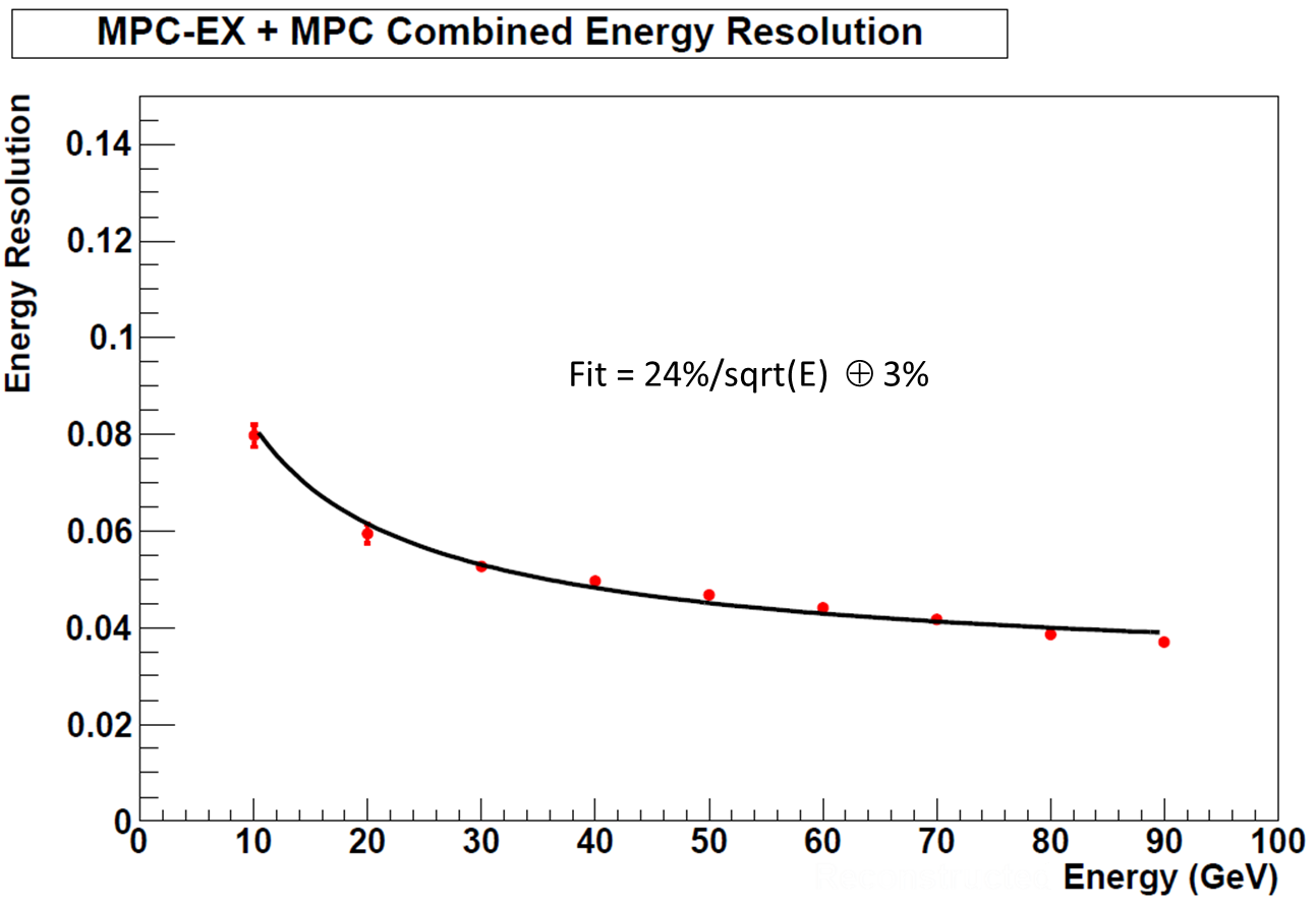
Figure 3.10: Energy resolution of the MPC-EX + MPC resonstruction in simulated events, using the calibration procedure outlined in the text. The large constant term in the resolution arises from combining MPC clusters with MPC-EX tracks. In the analysis of real data, a combined reconstruction will be used and it is anticipated that the energy resolution will improve.

3.2 EM Shower Reconstruction Performance: $\gamma$ and $\pi^{0}$.

3.2.1 Overview of Section

In this section, the reconstruction performance is evaluated and discussed in the context of single $\gamma$ and $\pi^{0}$ simulations. This is followed by a brief discussion of the performance in a simulation of the full $p+p$ cross-section using Pythia.

3.2.2 Basic cuts used in the reconstruction

In this analysis, a series of “basic cuts” are applied to all data to clean-up the event sample prior to more detailed analysis. These cuts are aimed at reducing effects due to poorly reconstructed electromagnetic showers, due to errors in the reconstruction or acceptance effects. The final product should be a sample of events which include all single-$\gamma$s and clusters of merged showers from $\pi^{0}$ decays.

The first cut separates tracks with a reconstructed energy of at least 20 GeV. Below this limit the number of $\pi^{0}$s which form two distinct MPC clusters increases, thus most tracks below this energy are single-$\gamma$’s and not overlapping $\pi^{0}$s. Such tracks can be used to reconstruct $\pi^{0}$s using a “two-track” method similar to that used in the current MPC-only analysis. Tracks with reconstructed energies greater than 20 GeV are subject to an additional analysis in a region of interest around the track to determine if the track is consistent with a single shower (a photon) or an overlap between photon showers (a $\pi^{0}$). This procedure is described in Section  3.2.3.

Only a preshower track that is tagged as “closest” to an MPC cluster is considered in the direct photon analysis. It is also required that the preshower track vector and the direction vector formed from the MPC cluster agree to within $\Delta({\rm Hough})$$<$0.0025 (distance in Hough space), see Figure 3.7.

Finally, a fiducial cut in $\eta$-space rejects tracks reconstructed close to the edge of the preshower. These are typically malformed and may, for example, have missing or distorted energy signals due to shower leakage. Figure 3.11 shows the pseudorapidity dependence of reconstructed tracks in a single-$\gamma$ simulation. The input $\eta$ was thrown over 2$<$$|\eta|$$<$4.5 (black histogram), and the full reconstruction was run. By selecting tracks with both an MPC and preshower component, with the latter being “closest”, the pseudorapidity coverage was found to be $\sim$3.1$<$$\eta$$<$$\sim$4.2 (red). The requirement of a minimum energy ($E_{\rm Rec}$$>$20 GeV) serves only to reduce statistics, as expected (blue).

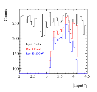
Figure 3.11: $\eta$ distribution of single-$\gamma$s from a simulation where the input distibution is wider than the acceptance of the detector (black). The reconstructed closest tracks (red) and those with a reconstructed energy greater than 20 GeV (blue) are shown.

Figure 3.12 shows the reconstructed energy (left panels) and $\eta$ (right panels) relative to the input value. The upper panels depict this versus the input $\eta$ for each event, and the lower panels show this versus the input energy. The black (red) histogram shows the distribution for $\gamma$s ($\pi^{0}$s). The accuracy of the reconstructed $\eta$ is found to degrade for low $\eta$ (worse for $\pi^{0}$s), whilst the energy reconstruction degrades only as a function of energy.

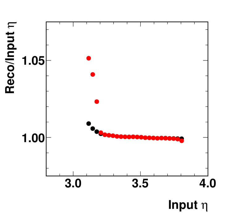
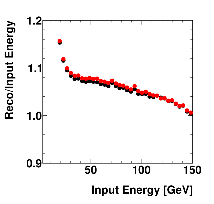
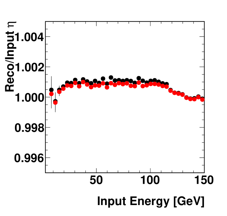
Figure 3.12: Reconstructed energy (left figures) and reconstructed $\eta$ (right) as a function of $\eta$ (top) and energy (bottom).

3.2.3 Single-track invariant mass calculation

Once an electromagnetic track candidate is found, it is tested to determine whether it is consistent with a single-electromagnetic shower or two close showers, similar to that expected from $\pi^{0}\rightarrow\gamma\gamma$ decays. Only high energy tracks (E$>$20 GeV) and the closest track to a single MPC cluster are considered. The process begins with a detailed examination of the minipad hits in a region of interest around the MPC-EX track. This region of interest is fixed at 0.0175 in Hough space in both the $x$ and $y$ directions, or a width of $\sim$41 minipads. A histogram of the minipad energies is then divided into two halves (performed independently for $x$- and $y$-minipads). In a first pass, the dividing line is the center of gravity of the energy distribution in each direction. This is subsequently changed in an iterative fashion until a small change in the split-point results in no change in the energy assigned to each track, i.e. a stable point is found. Typically, the stable point is found at the first or second iteration.

Once a stable point is found, the energy in the MPC-EX for each sub-track is determined, and the total energy of the track is shared between the subtracks based in these energy fractions. The subtracks can then be combined to form an invariant mass, which is associated with the MPC-EX track object. If all goes well, a single $\pi^{0}$ will be reconstructed into two subtracks, and those subtracks will reconstruct to the $\pi^{0}$ invariant mass.

It is important to note that the calculation of the invariant mass serves as both a method to identify and measure $\pi^{0}$s as well as a method to exclude $\pi^{0}$s from the direct photon analysis. If no invariant mass is found, then this is more likely to be a $\gamma$ candidate, rather than a $\pi^{0}$. However, a two-track decay does not necessarily produce two discernable tracks. This will be discussed further in the next section. The reconstruction of the invariant mass is quite aggressive at rejecting all candidates which do not appear as $\pi^{0}$s. This helps in reconstructing $\pi^{0}$s, and forces all “failed” invariant mass reconstruction into one of two categories.

The first category deals with candidates which have too few minipad hits associated with the track. Many tracks in this category fail due to a failure of the track matching between the MPC and MPC-EX, rather than due to too few hits in the pre-shower detector. Because of the resolution of the MPC it is possible to select a track which is a fluctuation from the main shower, but this happens to be the closest track in Hough space. In this scenario, there are too few hits in the MPC-EX to continue reconstruction simply from matching to the wrong track. This mode is greatly reduced by clustering tracks associated with a given MPC shower as described previously.

The second point of failure occurs when the algorithm cannot divide the energy up enough to separate two distinct peaks in the $x$- o̱r $y$-directions, i.e. no stable dividing point is found. The reason for this could be a real single-$\gamma$ (for example a signal photon), an asymmetrically decayed $\pi^{0}$, a track-matching failure whereby only one track (from a $\pi^{0}$ decay) falls in the acceptance.

As will be discussed in later sections, the performance of this algorithm on a given $\pi^{0}$ track depends greatly on the asymmetry of the event. For large asymmetries, the lower-energy photon can be buried under the shower from the higher energy photon. This results in an essentially symmetric shower, and the algorithm will either fail to converge on a dividing point in the shower, or a dividing point will be selected with a very small opening angle between the subtracks, resulting in a very low invariant mass. A shower due to a single photon will also be symmetric, and will reconstruct in a similar fashion, with the subtracks being determined by fluctuations in the photon shower. For this reason, we can define photon candidates as tracks that either fail the invariant mass reconstruction, or reconstruct to a very low mass. This is not a “true” invariant mass of the photon, but an artifact of the reconstruction. A photon sample defined in this way will be subject to contamination from $\pi^{0}$s that will have to be removed with additional cuts.

3.2.4 Reconstruction Performance

Position Resolution

The resolution and offset to the reconstructed track vector, relative to the input vector of the particle, for a single-$\gamma$ and single-$\pi^{0}$ simulations is shown in Figure 3.13. The left panel shows the $\eta$ resolution (open symbols) and offset (closed) for single-$\gamma$ and single-$\pi^{0}$ simulations.

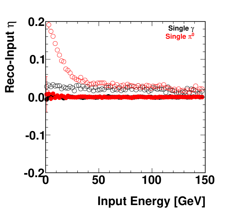
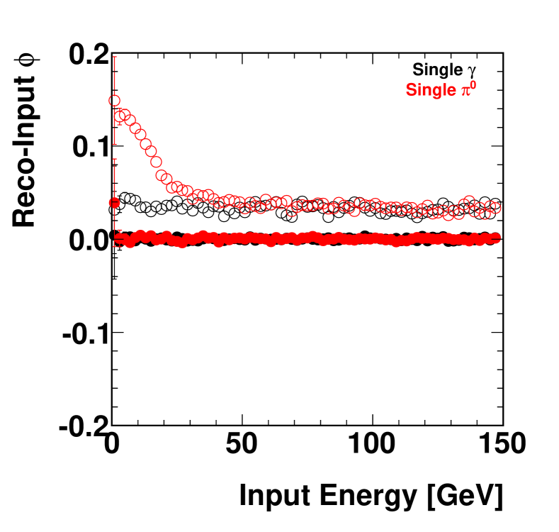
Figure 3.13: $\eta$ (left panel) and $\phi$ (right) resolution (open symbols) and offset (closed) for single-$\gamma$ (black) and single-$\pi^{0}$s. The deviation between $\pi^{0}$s and $\gamma$s observed at low energies is due to the reference $\eta$ (or $\phi$) following the original $\pi^{0}$ – not the decay $\gamma$ which has a different vector.

Invariant Mass Reconstruction

Candidate tracks in full events originate from a variety of sources. The dominant source is $\pi^{0}$s which can appear as two independent tracks in the detector (two-track $\pi^{0}$s) or merged as a single cluster (as seen in the MPC). The aim of the analysis in this document is to measure the production of direct-$\gamma$s, whose dominant background source is the $\pi^{0}$. Thus, $\pi^{0}$s must be measured to enable the extraction of direct-$\gamma$s. The measurement of the $\pi^{0}$ cross-section is not less important, but is not the focus here. Other sources, for example charged hadrons, $\eta$ mesons, and other decay photon sources are discussed in more detail in Section 3.2.8.

Figure 3.14 shows the reconstructed invariant mass versus the reconstructed energy for single input $\gamma$s (left) and $\pi^{0}$s (right). A cut in the reconstruction at $E$ = 20 GeV is applied, as below this energy two distinct tracks are typically found in the detector. A more detailed view of this can be found in Figs. 3.15 to 3.21, where slices in reconstructed energy are made in $\Delta E$ = 5 GeV bins. Figure 3.15 (left) shows the 20$<$$E_{\rm Rec}$$<$25 GeV bin. The red histogram shows single-$\pi^{0}$s, where a small correct-mass peak is observed, black shows single-$\gamma$s reconstructed at the same energy. A low-mass tail is observed for single-$\pi^{0}$s which is due to the reconstruction algorithm picking up a fluctuation in energy from a single shower and thus reconstructing a mass based from one $\gamma$. The normalization of the two histograms was chosen to fix the maximum height to be the same. Figure 3.15 (right) shows the 25$<$$E_{\rm Rec}$$<$30 GeV bin. A more prominant correct-mass peak is observed. At higher reconstructed energies, the correct-mass peak becomes dominant and the low-mass peak shrinks (relatively). The overall low mass peak distribution, however, still retains the same shape as that from single-$\gamma$s.

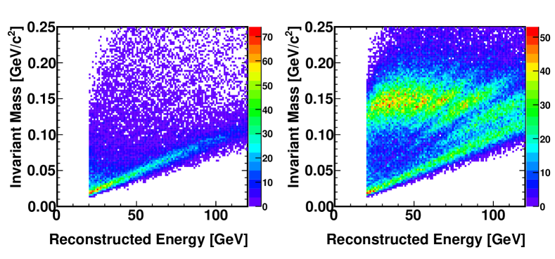
Figure 3.14: The left (right) panel shows the reconstructed invariant mass versus reconstructed energy for $\gamma$s ($\pi^{0}$s).

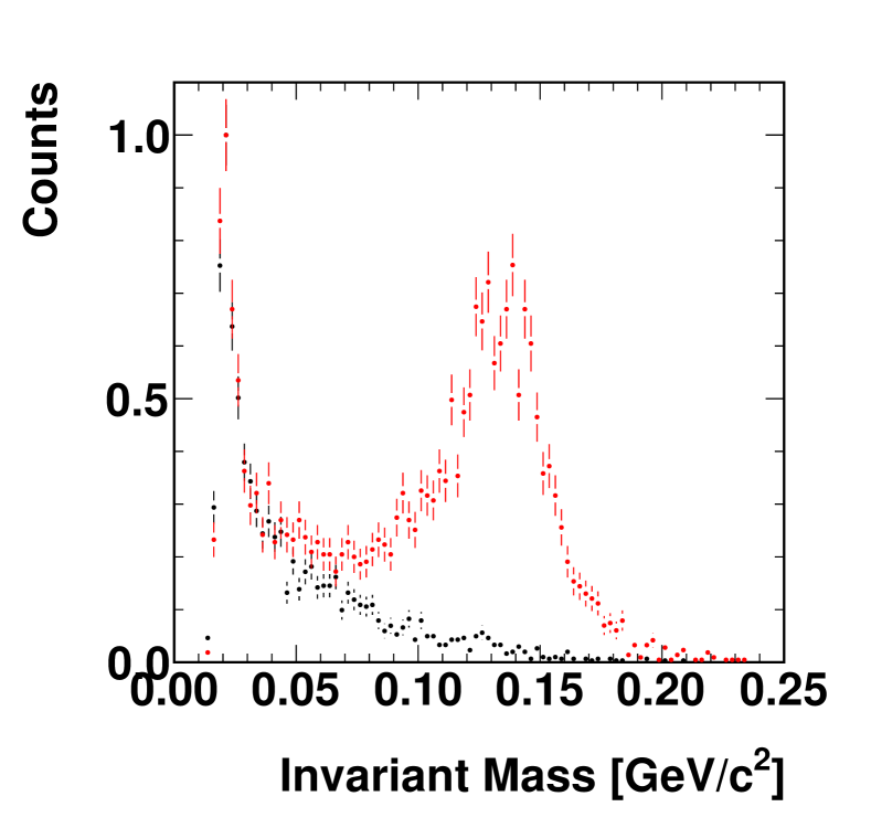
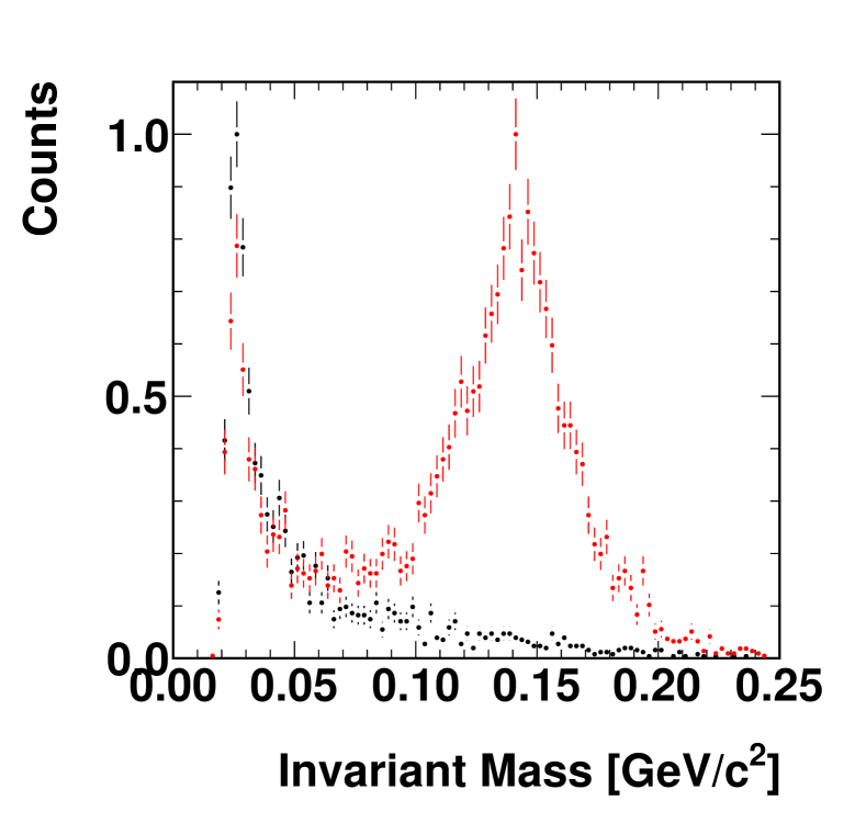
Figure 3.15: Comparison of the invariant mass distribution for $\gamma$s (black) and $\pi^{0}$s (red) for the 20$<$E$<$25 GeV (25$<$E$<$30 GeV) energy range. The normalization of the two histograms was chosen to fix the maximum height to be the same.

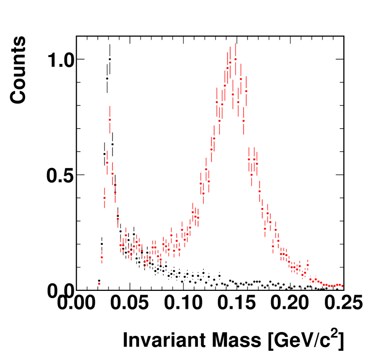
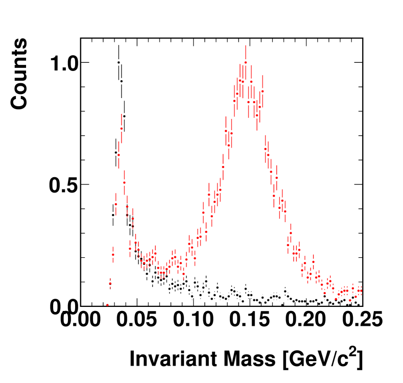
Figure 3.16: Comparison of the invariant mass distribution for $\gamma$s (black) and $\pi^{0}$s (red) for the 30$<$E$<$35 GeV (35$<$E$<$40 GeV) energy range.

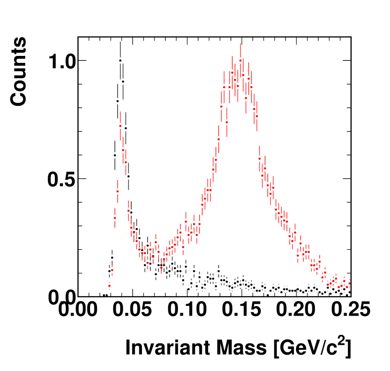
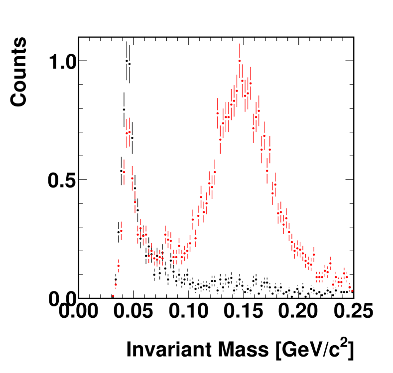
Figure 3.17: Comparison of the invariant mass distribution for $\gamma$s (black) and $\pi^{0}$s (red) for the 40$<$E$<$45 GeV (45$<$E$<$50 GeV) energy range.

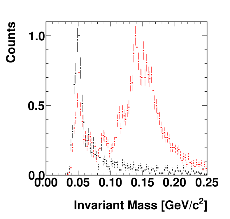
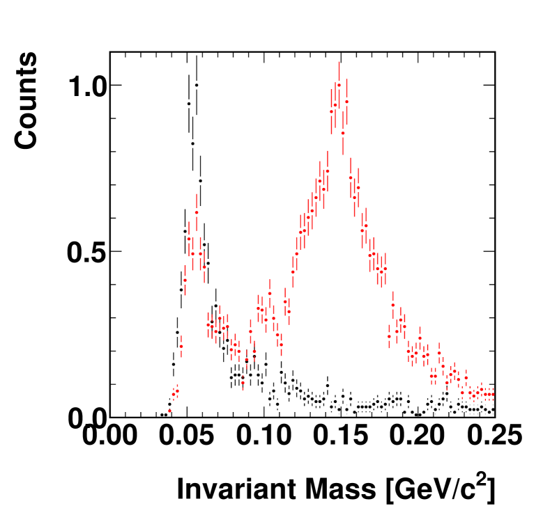
Figure 3.18: Comparison of the invariant mass distribution for $\gamma$s (black) and $\pi^{0}$s (red) for the 50$<$E$<$55 GeV (55$<$E$<$60 GeV) energy range.

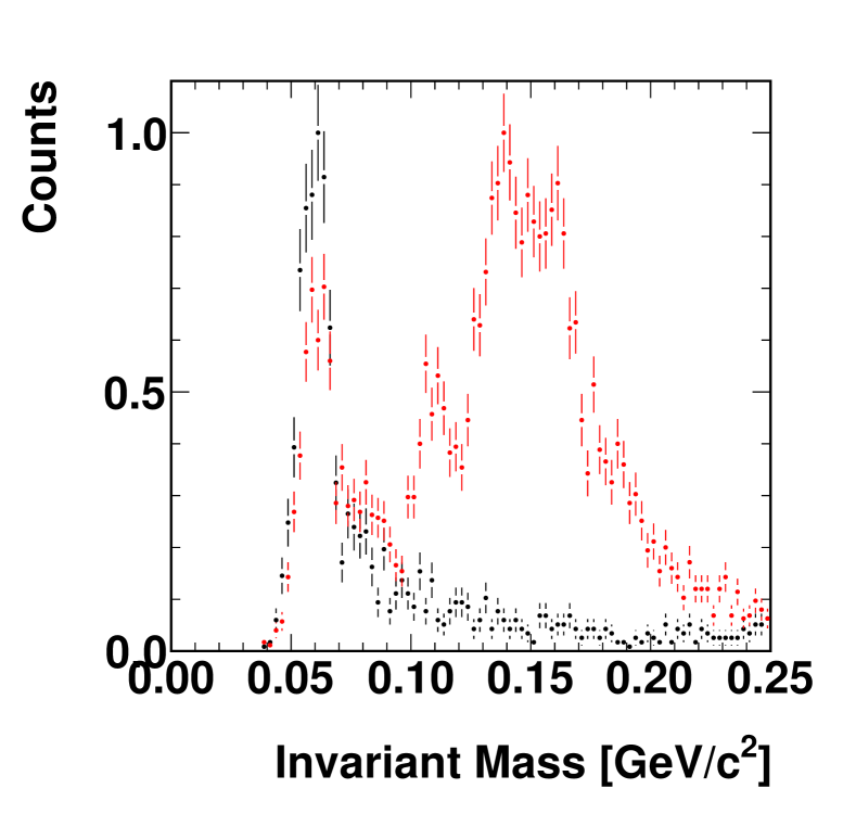
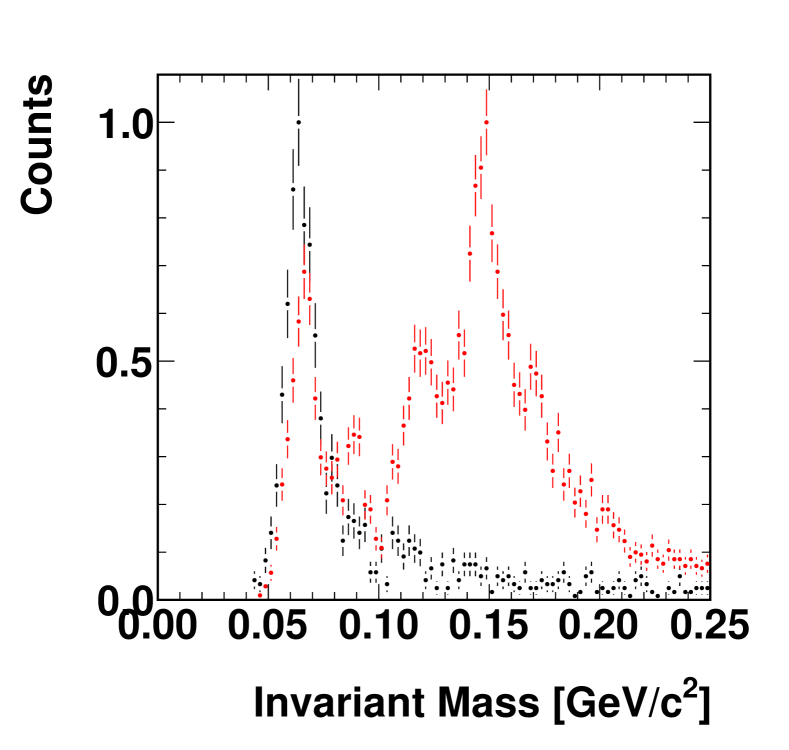
Figure 3.19: Comparison of the invariant mass distribution for $\gamma$s (black) and $\pi^{0}$s (red) for the 60$<$E$<$65 GeV (65$<$E$<$70 GeV) energy range.

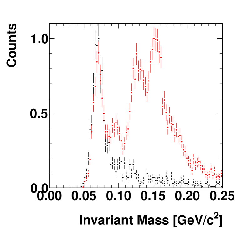
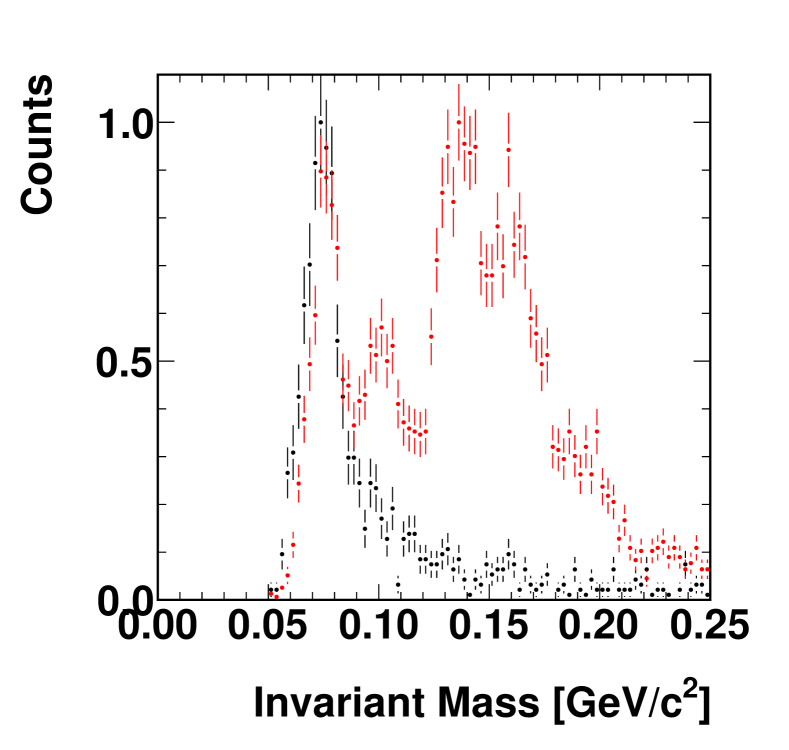
Figure 3.20: Comparison of the invariant mass distribution for $\gamma$s (black) and $\pi^{0}$s (red) for the 70$<$E$<$75 GeV (75$<$E$<$80 GeV) energy range.

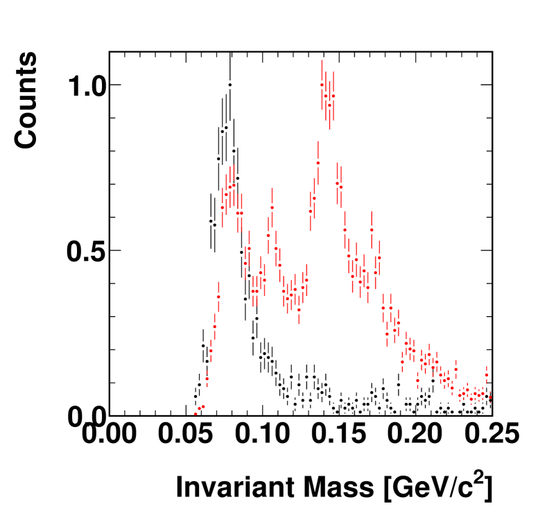
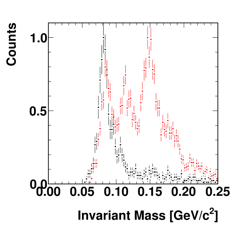
Figure 3.21: Comparison of the invariant mass distribution for $\gamma$s (black) and $\pi^{0}$s (red) for the 80$<$E$<$85 GeV (85$<$E$<$90 GeV) energy range.

Single-Particle Reconstruction Efficiencies

Table 3.2: Single-Particle Reconstruction Efficiency. The first column are the number of MC particles thrown into MPC-EX with the stated energy. The second column are the number in the reconstruction which passed all the cuts and have a reconstructed mass, note that there is no restriction on the incoming particle energy applied, so in- and out-flow are possible. The percentages in this column are relative to the input tracks. The next columns are the number of tracks at low/high reconstructed mass the percentages are “per reconstructed track”, i.e. “passed”.

Energy Range		Thrown	Passed	0$<$ Inv. Mass $<$0.06	Inv. Mass $>$0.06
$>$20 GeV	$\gamma$	147527	25071	9902	15169
		100%	16.9%	39.4%	60.5%
	$\pi^{0}$	148927	92298	8080	84218
		100%	61.9%	8.7%	91.2%
20-25 GeV	$\gamma$	9329	2611	1877	734
		100%	27.9%	71.8%	28.1%
	$\pi^{0}$	9247	5037	1456	3581
		100%	54.4%	28.9%	71%
25-30 GeV	$\gamma$	9268	2322	1623	699
		100%	25%	69.8%	30.1%
	$\pi^{0}$	9123	5615	1126	4489
		100%	61.5%	20%	79.9%
30-35 GeV	$\gamma$	9147	2074	1351	723
		100%	22.6%	65.1%	34.8%
	$\pi^{0}$	9234	6084	976	5108
		100%	65.8%	16%	83.9%
35-40 GeV	$\gamma$	9200	1847	1126	721
		100%	20%	60.9%	39%
	$\pi^{0}$	9338	6332	941	5391
		100%	67.8%	14.8%	85.1%
40-45 GeV	$\gamma$	9204	1727	975	752
		100%	18.7%	56.4%	43.5%
	$\pi^{0}$	9318	6476	858	5618
		100%	69.4%	13.2%	86.7%
45-50 GeV	$\gamma$	9210	1618	862	756
		100%	17.5%	53.2%	46.7%
	$\pi^{0}$	9385	6331	789	5542
		100%	67.4%	12.4%	87.5%

Table 3.3: Continuation of Tbl. 3.2.

Energy Range		Thrown	Passed	0$<$ Inv. Mass $<$0.06	Inv. Mass $>$0.06
50-55 GeV	$\gamma$	9148	1495	751	744
		100%	16.3%	50.2%	49.7%
	$\pi^{0}$	9348	6292	706	5586
		100%	67.3%	11.2%	88.7%
55-60 GeV	$\gamma$	9164	1535	612	923
		100%	16.7%	39.8%	60.1%
	$\pi^{0}$	9238	6258	590	5668
		100%	67.7%	9.4%	90.5%
60-65 GeV	$\gamma$	9441	1453	391	1062
		100%	15.3%	26.9%	73%
	$\pi^{0}$	9197	6068	383	5685
		100%	65.9%	6.3%	93.6%
65-70 GeV	$\gamma$	9103	1399	192	1207
		100%	15.3%	13.7%	86.2%
	$\pi^{0}$	9312	5923	169	5754
		100%	63.6%	2.8%	97.1%
70-75 GeV	$\gamma$	9166	1355	81	1274
		100%	14.7%	5.9%	94%
	$\pi^{0}$	9375	6007	66	5941
		100%	64%	1%	98.9%
75-80 GeV	$\gamma$	9142	1290	38	1252
		100%	14.1%	2.9%	97%
	$\pi^{0}$	9423	5677	15	5662
		100%	60.2%	0.2%	99.7%
80-85 GeV	$\gamma$	9270	1222	13	1209
		100%	13.1%	1%	98.9%
	$\pi^{0}$	9415	5470	5	5465
		100%	58%	0%	99.9%
85-90 GeV	$\gamma$	9320	1144	10	1134
		100%	12.2%	0.8%	99.1%
	$\pi^{0}$	9305	5141	0	5141
		100%	55.2%	0%	100%

3.2.5 Shower Shape

Candidate tracks in the MPC-EX are compared to a shower library in order to provide an additional discrimination between true photon showers, and sources of background (such as high energy $\pi^{0}$s). A shower library was developed from a sample of single-particle photon showers in the MPC-EX, and indexed by energy and by the layer of first interaction in the MPC-EX. This depth information is important because the MPC-EX is seeing the electromagntic shower in its infancy, and a shower that developed late in the MPC-EX will have a very different profile than a shower that starts in the first layers of the MPC-EX, and it is in this way that depth information from the MPC-EX is incorporated into the reconstruction. The shower profiles are kept separately for the $x$ and $y$ oriented minipads.

MPC-EX tracks are compared to the shower profiles using the Kolmogorov test [1], which is a statistical method for determining if two distribution are consistent with being drawn from the same underlying probability distribution. The Kolmogorov test returns this information as a “distance” value that characterizes the comparison - a large distance indicates a smaller probability that two two distributions are compatible.

Every MPC-EX track with $E>$20 GeV is compared to the reference shower library for the initial shower depth and reconstructed energy, and the corresponding Kolmogorov distances are recorded with the track object. Figure 3.22 shows the Kolmogorov distances for the $x$ and $y$ minipads for a sample of single $\pi^{0}$ and photons showers in the MPC-EX. It can be seen that the shower shape comparison can provide some discrimination between photon and high energy $\pi^{0}$ showers, especially when the distance in both projections are combined (see the direct photon analysis, Section 3.2.8). Of course, the power of a shape cut is limited in the MPC-EX because it only sees a fraction of the electromagnetic shower development. Additional cuts on the MPC shower shape are also used in the direct photon analysis (see Section 3.2.8).

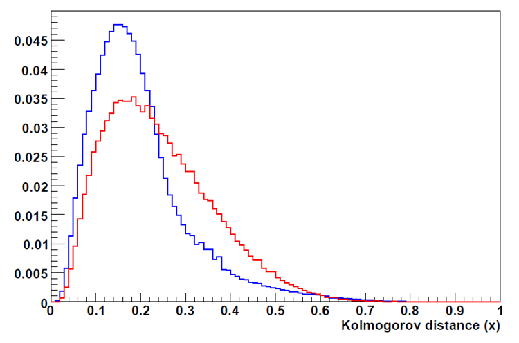
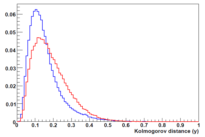
Figure 3.22: The Kolmogorov distance distributions for $\pi^{0}$s (red) and photons (in blue). Both distributions are normalized to the same area (number of events). The difference in two projections is driven by the fact that the $y$ projection minipads are always after the $x$ projection minipads.

3.2.6 $\chi^{2}$ Calibration

The $\chi^{2}$ calibration is an important piece of the electromagnetic shower reconstruction. The purpose is to remove contamination from charged hadrons, which may masquerade as electromagnetic showers. Electromagnetic showers are distinct as, for a given energy, the shower profile is somewhat predictable. For charged hadrons, the shower profile is different, sometimes a shower develops, sometimes only MIPs are seen in the silicon. Here we are primarily concerned with removing charged hadrons that begin showering in the MPC-EX.

A $\chi^{2}$ is formed to characterize the shower profile at each layer in the silicon with the aim to reduce the charged hadron contamination. Both the energy deposited and the transverse profile of the shower in each layer are measured for many events, then the mean and RMS of those distributions are found as references. Figures 3.23 and 3.24 show the mean and RMS of the calibration, versus collision energy, for the energy deposition profile and transverse profile respectively. The calibration is performed twice, once for single-$\gamma$s, and again as a cross-check with single-$\pi^{0}$s. The energy deposition, as expected, is very similar for the two cases, as both are electromagnetic showers. However, the width is distinct, as the $\pi^{0}$ showers are from two separated $\gamma$s. For higher reconstructed energies, those distributions start to approach each other, as the angular separation diminishes.

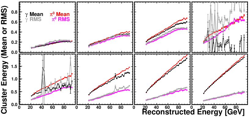
Figure 3.23: Calibration of the energy deposition profile for a reconstructed track. The calibration is performed using single-$\gamma$s and single-$\pi^{0}$s. The top row (left to right) show the layers 0 through 3, the bottom row 4 through 7. The black/grey symbols show the mean/RMS of the single-$\gamma$ distribution. The red/purple symbols show the mean/RMS of the single-$\pi^{0}$ distribution.

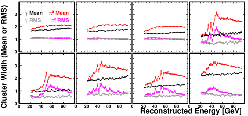
Figure 3.24: Calibration of the transverse profile at each layer for a reconstructed track. The calibration is performed using single-$\gamma$s and single-$\pi^{0}$s. The top row (left to right) show the layers 0 through 3, the bottom row 4 through 7. The black/grey symbols show the mean/RMS of the single-$\gamma$ distribution. The red/purple symbols show the mean/RMS of the single-$\pi^{0}$ distribution.

Four final $\chi^{2}$ methods have been developed for this analysis, with varying degrees of success. Two (one in energy, the other in width) are based on the $\chi^{2}$ formed from all layers, and a second pair is derived from only the last 3 layers, where the showers are more definitely defined. As an example, Fig 3.25 shows the four cases for the lowest energy considered (20.0$<$$E_{\rm Rec}$$<$22.5 GeV). Energy bins 40.0$<$$E_{\rm Rec}$$<$42.5 GeV, 60.0$<$$E_{\rm Rec}$$<$62.5 GeV, and 80.0$<$$E_{\rm Rec}$$<$82.5 GeV are shown in Figs. 3.26, 3.27, and 3.28 respectively.

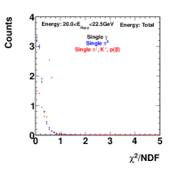
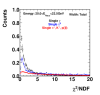
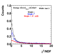
Figure 3.25: $\chi^{2}$ calibration applied to single-$\gamma$s (black), single-$\pi^{0}$s (red), and single-charged hadrons (mixed $\pi^{\pm}$, $K^{\pm}$, and $p(\overline{p})$), with reconstructed energy of 20$<$$E_{\rm Rec}$$<$22.5 GeV. Left to right, the panels show the calibration using energy (all layers), energy (last 3 only), width (all layers), and width (last 3 only).

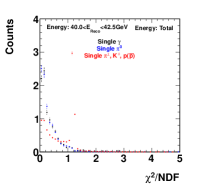
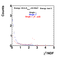
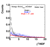
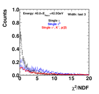
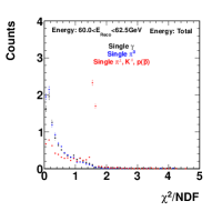
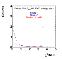
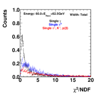
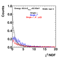
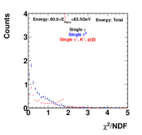
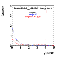
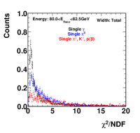
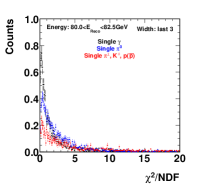
Figure 3.26: $\chi^{2}$ calibration applied to single-$\gamma$s (black), single-$\pi^{0}$s (red), and single-charged hadrons (mixed $\pi^{\pm}$, $K^{\pm}$, and $p(\overline{p})$), with reconstructed energy of 40$<$$E_{\rm Rec}$$<$42.5 GeV. Left to right, the panels show the calibration using energy (all layers), energy (last 3 only), width (all layers), and width (last 3 only).

Figure 3.27: $\chi^{2}$ calibration applied to single-$\gamma$s (black), single-$\pi^{0}$s (red), and single-charged hadrons (mixed $\pi^{\pm}$, $K^{\pm}$, and $p(\overline{p})$), with reconstructed energy of 60$<$$E_{\rm Rec}$$<$62.5 GeV. Left to right, the panels show the calibration using energy (all layers), energy (last 3 only), width (all layers), and width (last 3 only).

Figure 3.28: $\chi^{2}$ calibration applied to single-$\gamma$s (black), single-$\pi^{0}$s (red), and single-charged hadrons (mixed $\pi^{\pm}$, $K^{\pm}$, and $p(\overline{p})$), with reconstructed energy of 80$<$$E_{\rm Rec}$$<$82.5 GeV. Left to right, the panels show the calibration using energy (all layers), energy (last 3 only), width (all layers), and width (last 3 only).

Using these calibrations, one can define a $\chi^{2}$ cut for each of the methods. Figure 3.29 shows the cut positions, as a function of reconstructed energy, which keeps about 90% of the single $\gamma$s. The effect applying these cut to the single-$\pi^{0}$s, and single-charged hadrons is shown in Figure 3.30 (energy $\chi^{2}$) and Figire 3.31 (width $\chi^{2}$) as a fraction of the total which were reconstructed.

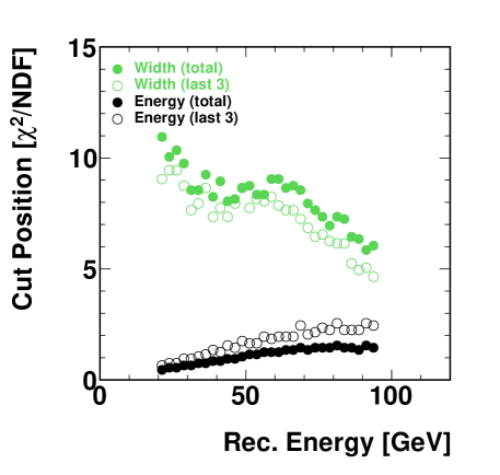
Figure 3.29: $\chi^{2}$ cut positions, determined to retain 90% of single-$\gamma$s for the energy (black) and width (green) methods. “Total” and “last 3” are depicted as closed and open symbols respectively.

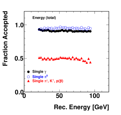
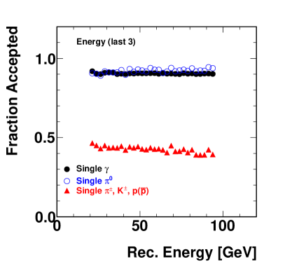
Figure 3.30: Fraction of single-$\gamma$s (black), single-$\pi^{0}$ (blue), and charged hadrons (red) retained by the energy total (right panel) and last 3 method (left). The cut position was set such that 90% of single-$\gamma$ passed the cuts.

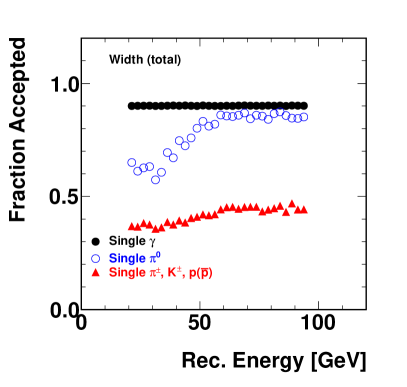
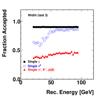
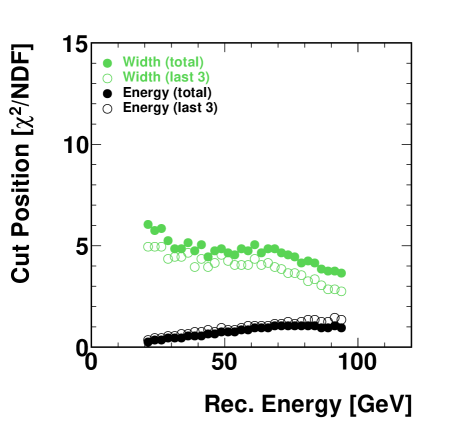
Figure 3.31: Fraction of single-$\gamma$s (black), single-$\pi^{0}$ (blue), and charged hadrons (red) retained by the width total (right panel) and last 3 method (left). The cut position was set such that 90% of single-$\gamma$ passed the cuts.

Figure 3.32: $\chi^{2}$ cut positions, determined to retain 80% of single-$\gamma$s for the energy (black) and width (green) methods. “Total” and “last 3” are depicted as closed and open symbols respectively.

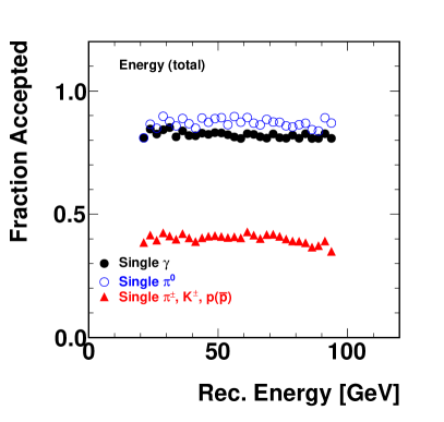
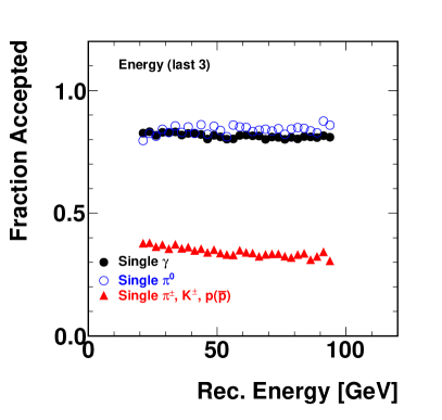
Figure 3.33: Fraction of single-$\gamma$s (black), single-$\pi^{0}$ (blue), and charged hadrons (red) retained by the energy total (right panel) and last 3 method (left). The cut position was set such that 80% of single-$\gamma$ passed the cuts.

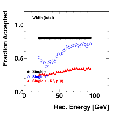
Figure 3.34: Fraction of single-$\gamma$s (black), single-$\pi^{0}$ (blue), and charged hadrons (red) retained by the width total (right panel) and last 3 method (left). The cut position was set such that 80% of single-$\gamma$ passed the cuts.

The $\chi^{2}$ for any event sample is then calculated relative to those references, and summed over each layer.

3.2.7 Reconstruction in Pythia events

Moving on from single-particle simulations, a full Pythia simulation was made to check for reconstruction features in a $p+p$ scenario. To gain a full understanding of the reconstruction, we match the closest match particle produced from Pythia and also the next-closest (to study effects due to track merging). The matching resolution between the reconstruction and Pythia is 0.13 in $\delta\eta$ and 0.05 in $\delta\phi$, see Figure 3.35.

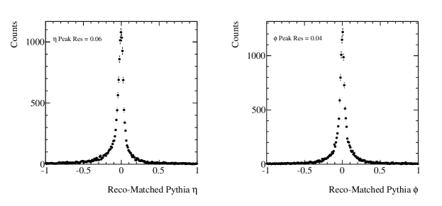
Figure 3.35: Resolution of matching between reconstructed and Pythia primary particles. The left panel shows the $\delta\eta$ resolution and the right shows the $\delta\phi$ resolution. The text states the Gaussian sigma of a fit to a region close to the peak, to exclude the outliers.

$\pi^{0}$ Reconstruction

The reconstruction of $\pi^{0}$s is critical in determining the direct-$\gamma$ yields, as this is the largest contribution to the background. The reconstruction algorithms are well understood in single-particle events and are observed to find high-$p_{T}$ $\pi^{0}$s. In Pythia, the addition of more particles, thus more energy in the MPC and preshower, could cause the algorithm to fail. This section discusses this behavior of the reconstruction method in the environment of a full Pythia event.

Figure 3.36 shows the reconstructed invariant mass in several bins of $p_{T}$; no quality-control cuts have been applied to the data – this is discussed later. In each panel, the black histogram shows the reconstructed data without knowing the origin of the particle which makes that track. Tracks which were created from $\pi^{0}$s are shown in red and, as expected, dominate the data. The legend in the figure denotes the fraction of all events in the given $p_{T}$ bin. The first number is the fraction which passed all reconstruction cuts, but ignores the value determined for the invariant mass. The second number shows the fraction of that particular particle with a well-reconstructed invariant mass tracks (i.e. $Inv.Mass$$>$0, indicating that the reconstruction did not succeed). The final number shows the fraction of that particular particle which did not produce a well-reconstructed invariant mass. The numbers are summarized in Table 3.4. Further in the Figure, more minor contributions to the total histogram are shown, specifically, the $\eta$ and low-mass vector mesons contribute a significant fraction and are a further source of background to the direct-$\gamma$s.

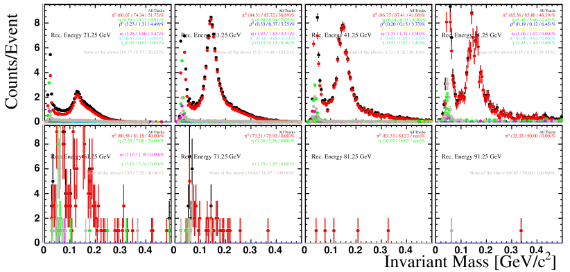
Figure 3.36: Reconstruction of all particles, showing the well reconstructed mass range. Numbers in the caption are: fraction of total / InvMass$>$0 (single track reconstruction converged) / InvMass$<$0 (single tracks reconstruction did not converge). The different panels show the energy dependence.

Table 3.4: Breakdown by particle type of the contribution to the invariant mass spectrum. No cut refers to the all data (irrespective of whether the invariant mass was reconstructed or not. ($<$0) $\geq$0 are tracks with a (not) well reconstructed invariant mass. “–” denotes too low statistics to be reliable. No quality-control cuts are applied to this data.

Energy	Invariant	$\pi^{0}$	$\eta$	$\rho^{0}$	$\rho^{+}$	$\omega$	$\Delta^{+}$	$\gamma$	Something
GeV	Mass	%	%	%	%	%	%	%	Else (%)
20-22.5	No Cut	60.7	9.4	3.2	3.0	3.3	0.63	0.02	19.8
	$\geq$0	74.3	10.1	1.3	1.3	3.0	0.31	0.03	9.6
	$<$0	51.8	8.9	4.5	4.1	3.5	0.84	0.01	26.4
30-32.5	No Cut	84.3	6.9	0.53	0.53	1.9	0.11	0.15	5.5
	$\geq$0	85.7	6.9	0.37	0.39	1.9	0.08	0.15	4.5
	$<$0	39.9	7.1	5.8	5.2	3.5	1.4	0.46	40.0
40-42.5	No Cut	86.8	6.1	0.20	0.26	1.3	0.05	0.55	4.7
	$\geq$0	87.4	6.1	0.15	0.21	1.3	0.03	0.52	4.3
	$<$0	41.1	8.3	3.7	4.2	2.9	1.2	2.5	36.1
50-52.5	No Cut	85.4	5.4	0.19	0.12	1.0	0.04	1.43	6.5
	$\geq$0	85.8	5.4	0.12	0.08	1.0	0.04	1.45	6.1
	$<$0	48.4	6.5	6.5	3.2	–	–	–	35.5
60-62.5	No Cut	80.6	7.3	–	–	1.2	–	3.19	7.8
	$\geq$0	81.2	7.1	–	–	1.2	–	3.24	7.4
	$<$0	–	–	–	–	—	–	–	–
70-72.5	No Cut	73.2	–	–	–	–	–	1.8	19.6
	$\geq$0	75.9	–	–	–	–	–	1.9	16.7
	$<$0	–	–	–	–	–	–	–	–
80-82.5	No Cut	83.3	–	–	–	–	–	–	–
	$\geq$0	83.3	–	–	–	–	–	–	–
	$<$0	–	–	–	–	–	–	–	–
90-92.5	No Cut	33.3	–	–	–	–	–	–	–
	$\geq$0	50.0	–	–	–	–	–	–	–
	$<$0	–	–	–	–	–	–	–	–

Figures 3.37 (linear scale) and 3.38 (logarithmic scale) show a summary of the simulated data from Figure 3.36 / Table 3.4. The left panels show the fraction of well reconstructed invariant mass data relative to the total number of tracks reconstructed. The right show the fraction that do not reconstruct to an invariant mass. The data at high energy are statistics starved; additionally, there are no quality-control cuts applied. The fraction of $\gamma$ events rises steadiily from low-to-high energy as the cross-section of the hadronic sources drops.

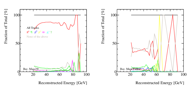
Figure 3.37: Energy dependence of fraction of each particle type, no cuts except fiducial cut.

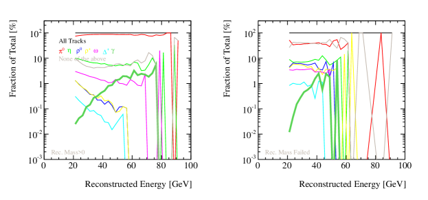
Figure 3.38: Same as Figure 3.37, but logarithmic scale on the y-axis for detail.

$\pi^{0}$ Reconstruction In Detail

The main problem in the analysis of the $\pi^{0}$s is a kinematic property of the decay of the $\pi^{0}$. In the rest frame of the $\pi^{0}$, the decay angle is evenly distributed. As such, the energy of each daughter $\gamma$, when boosted into the collision rest frame, is not equally. In fact, it is unusual for an equal energy for each $\gamma$. This is not a particular problem for the two-track analyses, but for single tracks, where the distance between tracks is small, the lesser-energy track can be overwhelmed by its counterpart to the degree that the signal is lost in the tails of the larger-energy $\gamma$. This can be illustrated by looking at the asymmetry of the decay versus the reconstructed invariant mass. Figure 3.39 shows this for the true decay asymmetry (left panel) and the estimated decay asymmetry based on the energy in the minipads associated to each track. For the true case, very asymmetric tracks mostly reconstruct as a ’single $\gamma$’ at low invariant mass. For tracks with an asymmetry of 50% or less (zero is equally-shared energy), the mass is amost always well reconstructed. The estimated asymmetry from the reconstructed mini-pad energy associated to each $\gamma$ does not reflect this. This is due to the small sampling fraction coupled with the optimization within the algorithm to separate the daughter $\gamma$s.

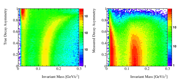
Figure 3.39: True (left) and measured (right) asymmetry versus the reconstructed invariant mass.

One can look at this in more detail with an energy dependence of the asymmetry, see Figure 3.40. One finds that the fraction of mis-reconstructed mass is highest in the low-energy bins, whilst at higher energy, the mass becomes better defined, even for very asymmetry decays.

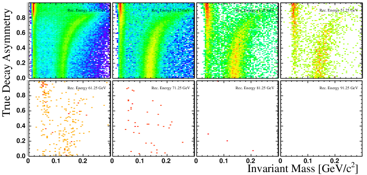
Figure 3.40: Energy dependence of true asymmetry versus invariant mass.

3.2.8 Track Selection Cuts in Pythia events

The Pythia simulation is analyzed to identify direct photon candidates. The event vertex must be within $\pm 50$ cm. Tracks must fall within the MPC-EX $\eta$ acceptance (3.1$<$$|\eta|$$<$3.8), match to a unique MPC cluster, and have an MPC-to-MPC-EX hough separation below 0.005. These requirements ensure that all surviving tracks have a similar acceptance, are properly reconstructed in the MPC-EX and are well matched to the MPC. The studies presented in this section apply these cuts to ensure that the sample contains to only well reconstructed tracks.

Pythia primary information is used to identify the source of a photon candidate tracks. Reconstructed tracks are associated to hadrons, $\pi^{0}$’s, decay photons, and direct photons. The Pythia association requires that the Pythia primary and reconstructed track are in the same arm and have a Hough space separation of less than 0.02. The Hough space separation between reconstructed tracks and the Pythia primaries in the $x$ and $y$ coordinates are shown in Figure 3.41. Tracks that fail to match to a Pythia primary are retained and classified as unassociated tracks. After hadron removal cuts are applied unassociated tracks are less than one percent of the remaining yield.

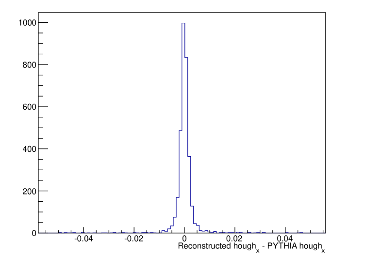
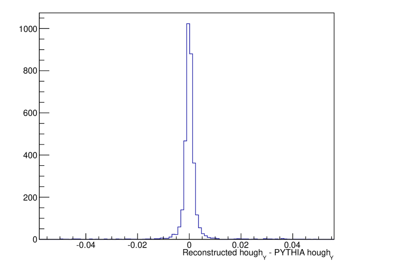
Figure 3.41: The separation between reconstructed tracks and the Pythia associated tracks in Hough space for the $x$- (left) and $y$-coordinate (right) in a subset of the simulated data sample.

Using the Pythia association, photons can be separated into one of two categories: direct photons from the initial hard scattering and fragmentation photons from outgoing quark fragmentation. For the remainder of this section, the term “signal photons” refers to the sum of these sources. There is also a third source of photons from QED radiation off of the incoming quark lines. These are produced in the Pythia simulation. However, the amount of QED radiation is much larger than what is expected from NLO rate calculations. As a result we have excluded this contribution from our analysis. We are working with theorists to understand the proper reweighting of the Pythia components to ensure agreement with NLO calculations. This is discussed in more detail in Section 3.3.

The direct photon measurement must contend with large backgrounds from hadrons, $\pi^{0}$’s and decay photons. Decay photons primarily consist of $\eta$ decays, with a small contribution from $\omega$ and $\eta$’ decays. The first step in this analysis is to remove as much of the hadron, $\pi^{0}$ and decay photon backgrounds as possible. The remaining backgrounds are removed through a double ratio calculation. The double ratio method is discussed in detail in Section 3.4.

The goal of the direct photon measurement is to determine the gluon contribution to direct photons using the measured $R_{dA}$ suppression. Direct photons from the initial hard interaction are more sensitive to suppression in the quark-gluon production mechanism than fragmentation photons radiated later in the collision. Isolations cuts and tighter cuts on the MPC and MPC-EX variables reduce the fragmentation photon contribution to the signal photon measurement.

In this section, we present the cuts used to identify direct photon candidates. These cuts remove the hadronic tracks, reduce the $\pi^{0}$ and decay photon backgrounds, and lessen the fragmentation photon contribution. The relevant variables are discussed and their distributions and cut efficiencies are shown. The efficiencies of the photon candidate tracks with all of the direct photon identification cuts applied are given at the end of this section.

Hadronic background

The hadronic background is reduced using event characteristics and cuts that distinguish between hadronic tracks and electromagnetic showers in the MPC-EX. In a direct photon event, the direct photons are the highest energy particles in the event. By considering only the highest energy track in each event, 81.6% of the hadron tracks are removed with only a 3% reduction in the signal photon yields. Since the backgrounds are largest at low $p_{T}$, we require the $p_{T}$ to be greater than 3 GeV and reduce the background contribution in the sample significantly. This is particularly effective for the hadron and $\pi^{0}$ backgrounds both of which drop by over 99.5%. As charged hadrons pass through the MPC-EX, they deposit a small amount of their energy in the layers of the MPC-EX. To remove these tracks we reject all candidates that deposit less than the minimum ionizing energy of 0.07 GeV in a narrow region of interest and tracks with fewer than two layers of the MPC-EX hit. The MIP requirement removes 62.9% of hadrons and 2.7% of signal photons. Figure 3.42 shows the efficiency of all of the hadron rejection cuts as a function of $p_{T}$. Over the entire $p_{T}$ range hadrons and unassociated tracks are reduced by 92.7% and 85.9%. $\pi^{0}$, $\eta$ and other decays drop by 65.2%, 66.3% and 64.5% respectively. Only 5.1% of direct photons are affected.

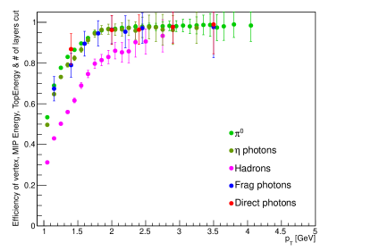
Figure 3.42: The efficiency distribution of the higest energy, MIP energy, vertex and number of MPC-EX layers cuts as a funtion of $p_{T}$. $\pi^{0}$ and $\eta$ are shown in bright and olive green respectively. Hadrons are shown in pink. Direct photons from the initial hard interaction are in red and fragmentation photons are in dark blue.

The remainder of this section focuses on removing $\pi^{0}$ and fragmentation photons. The hadron rejection cuts are applied throughout. Cuts designed to remove $\pi^{0}$ and fragmentation photons further reduce the small backgrounds from hadronic tracks.

$\pi^{0}$ background

The $\pi^{0}$ background is removed with a variety of cuts on the energy characteristics and shower widths in the MPC-EX and MPC. The track’s shower width is considered and a shower shape comparison to a single particle distribution is made using a Kolmogrov test [1]. The ratio of the track’s energy to the amount of energy deposited in a cone surrounding the track is used to separate isolated tracks from hadrons and $\pi^{0}$ in a jet. These variables and their distributions are presented below. The specific variable cut ranges are determined by using a multivariate analysis presented later in this section.

The shower width is characterized in the MPC-EX using the root mean square (RMS) of the energy distribution. The energy distributions are considered separately for the combined x and y layers and are summed in quadrature, $RMS=\sqrt{RMS_{X}^{2}+RMS_{Y}^{2}}$, where $RMS_{X}$ and $RMS_{Y}$ are the RMS of the showers in the x and y layers. In the MPC, shower widths are determined using the dispersion of the shower shape in the MPC clusters. The MPC dispersion in the $x$ and $y$ directions are combined, $disp=\sqrt{(\log(dispx))^{2}+(\log(dispy))^{2}}$. Figure 3.43 presents the MPC-EX RMS and MPC dispersion distributions for charged hadrons, $\pi^{0}$ and direct and fragmentation photons. Hadrons and $\pi^{0}$’s peak at and extend out to higher values than the direct photons in both variables. This shift allows us to separate the $\pi^{0}$ and remaining hadrons from the direct photons. A small shift is seen in the narrow peak of the $\pi^{0}$ dispersion distribution with a shoulder at $p_{T}$ greater than 2 GeV. The separation between the direct photons and $\pi^{0}$’s is more pronounced in the RMS distribution however the distribution is also a wider.

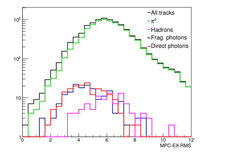
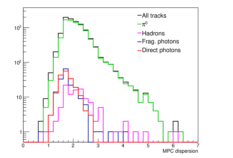
Figure 3.43: The the MPC-EX RMS and MPC dispersion distributions. The right panel shows the RMS and the left panel shows the dispersion. Direct photon are shown in red and fragmentation photons are in blue. Hadrons and $\pi^{0}$ tracks are in pink and green respectively. The sum of all tracks is shown in black.

The Kolmogorov test compares the expected shower shape of the candidate track with those from single particle $\pi^{0}$ simulations by calculating the distance between the two energy profiles. The Kolmogorov test is performed separately on the combined x layers and y layers. These values are restricted between zero and one and are summed in quadrature creating the KTestDist variable. Figure 3.44 displays the KTestDist distribution for all tracks, $\pi^{0}$, hadrons and fragmentation and direct photons. The direct and fragmentation photon distributions are peaked near a value of 0.2 and the $\pi^{0}$ distribution peaks at a value above 0.3.

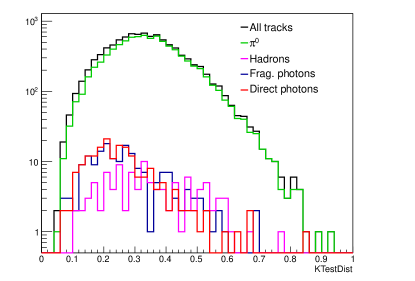
Figure 3.44: The distribution of the Kolmogorov test variable (KTestDist) as a function of $p_{T}$. The right panel shows the efficiency for with MPC energies and the left panel MPC-EX energies. Direct photon are shown in red and fragmentation photons are in blue. Hadron and $\pi^{0}$ tracks are in pink and green respectively. The sum of all tracks is shown in black.

Ratios of the track’s energy to the amount of energy deposited in a one radius cone in $\eta$-$\phi$ space surrounding the track are calculated separately for the MPC and MPC-EX energies. Figure 3.45 shows both of these distributions for all tracks, $\pi^{0}$, hadrons and fragmentation and direct photons. These ratios are peaked near one for all particles. Values of one occur when the photon candidate track is isolated and is the only source of energy in the cone. The distribution of the MPC ratio peaks slightly below one and extends to values above one. This is because the MPC energy of the track is the MPC cluster energy, while the MPC energy in the cone is uncalibrated and unclustered.

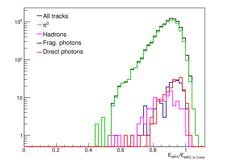
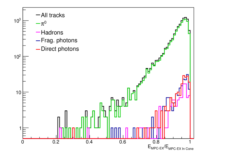
Figure 3.45: The distribution of the energy ratio in cone cuts with the energy in the MPC and MPC-EX as a function of $p_{T}$. The right panel shows the efficiency for with MPC energies and the left panel MPC-EX energies. Direct photon are shown in red and fragmentation photons are in blue. Hadrons and $\pi^{0}$ are shown in pink and green respectively. The sum of all tracks is shown in black.

Before cutting on these variables, we first remove known $\pi^{0}$’s from our sample. The single track invariant mass variable provides this rejection. The calculation of the single track invariant mass is discussed in detail in Section 3.2.3. The mass distributions for $\pi^{0}$’s, hadrons and fragmentation and direct photons are shown in Figure 3.46. The $\pi^{0}$’s have a clear peak at the pion mass and a low mass peak at 0.04 GeV. This low mass peak occurs when the mass reconstruction algorithm identifies an energy fluctuation as the basis for the second photon in the $\pi^{0}$ decay. The low mass peak is seen in all particle types. A cut requiring a single track mass below 0.06 GeV removes the properly reconstructed $\pi^{0}$ while retaining the direct photons in the low mass peak. The efficiency of this cut is also shown in Figure 3.46 and listed in Table 3.6. Over 70.9% of high $p_{T}$ $\pi^{0}$’s are removed and high $p_{T}$ direct photons survive with 90.3% efficiency.

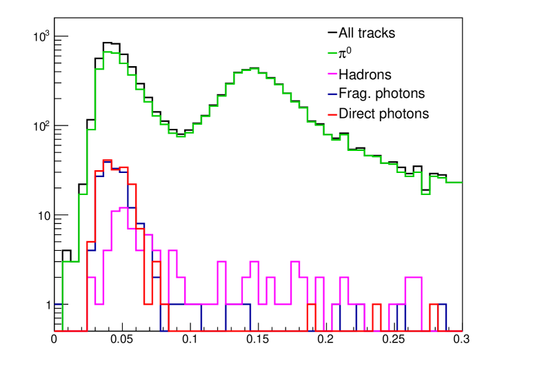
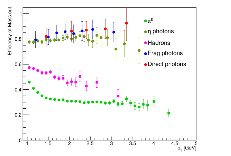
Figure 3.46: The single track invariant mass distributions of all high $p_{T}$ good tracks on the left and the efficiency of a $m<0.06$ GeV cut on the right. $\pi^{0}$ and $\eta$ are in light and olive green. Hadrons are in pink. Direct photons are in red and fragmentation photons are in blue.

A multi-variate analysis tool, TMVA, is used to determine the optimal cut locations of the MPC and MPC-EX variables to remove the $\pi^{0}$ background and maintain the direct photon signal [43]. This is performed on the $p_{T}>3$ GeV Pythia sample after the invariant mass and hadron cuts are applied. TMVA characterizes each of the variable distributions and dependencies for both the signal and background tracks. It determines optimal cuts for signal efficiencies between zero and one hundred percent with a one percent step size. Two rectangular cut algorithms are attempted in this study, the simulated annealing algorithm (CutsSA) and the genetic algorithm (CutsGA). Early studies also considered a Monte Carlo generation algorithm but this algorithm produced lower background rejections. The $\pi^{0}$ background is the only background considered in this TMVA analysis; the signal consists of both direct and fragmentation photons. Figure 3.47 presents the projected direct and fragmentation photon efficiencies versus $\pi^{0}$ rejection (ROC curve) for both algorithms. The CutsSA algorithm is used in this analysis. It consistently produces cuts within reasonable ranges and a more reliable and higher predictions of the signal efficiencies. The cuts determined by the CutsSA algorithm with a projected direct and fragmentation photon efficiency of $28\%$ and a projected $85\%$ rejection of $\pi^{0}$ are used and the corresponding acceptable variable ranges are listed in Table 3.5.

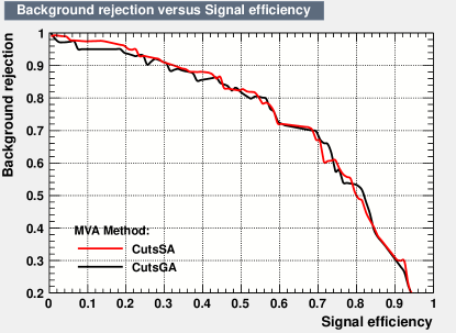
Figure 3.47: The signal efficiency versus background rejection curves (ROC curves) for the TMVA analysis of the direct and fragmentation photon signal and the $\pi^{0}$ background. The projected signal efficiencies and background rejections for the CutsSA and CutsGA curves are drawn in red and black respectively.

Table 3.5: Acceptable ranges for variables as defined by TMVA to remove the $\pi^{0}$ background.

Variable	Range
dispersion	0.812 - 1.631
RMS	0.663 - 6.118
KTestDistX	0.105 - 0.556
$E_{MPC-EX}/E_{MPC-EXInCone}$	$>$ 0.767
$E_{MPC}/E_{MPCInCone}$	0.727 - 1.013

Table 3.6: Efficiencies of the cuts in Table 3.5 for $\pi^{0}$, hadrons, direct and fragmentation photons for yields at $p_{T}>3$ GeV.

Variable	$\epsilon_{\pi^{0}}$	$\epsilon_{hadrons}$	$\epsilon_{\gamma frag}$	$\epsilon_{\gamma direct}$
Mass	$29.1\%$	$37.5\%$	$84.2\%$	$90.3\%$
dispersion	$8.6\%$	$9.6\%$	$35.0\%$	$35.5\%$
RMS	$51.9\%$	$48.1\%$	$81.4\%$	$84.4\%$
KTestDist	$48.3\%$	$58.4\%$	$61.0\%$	$71.5\%$
$E_{MPC-EX}/E_{MPC-EXInCone}$	$48.9\%$	$46.2\%$	$64.4\%$	$74.2\%$
$E_{MPC}/E_{MPCInCone}$	$49.2\%$	$47.1\%$	$65.5\%$	$74.2\%$
All $\pi^{0}$ cuts applied	$2.9\%$	$6.1\%$	$24.3\%$	$31.2\%$

Table 3.6 presents the efficiencies of each cut for $\pi^{0}$, hadrons, and direct and fragmentation photons above 3 GeV in $p_{T}$. Figures 3.48, 3.49 and 3.50, show the efficiencies for each of these cuts as a function of $p_{T}$ for $\pi^{0}$, hadrons and direct and fragmentation photons. All five variables are able to separate $\pi^{0}$ from direct and fragmentation photons. The dispersion cut has the lowest efficiency for both the signal photons and $\pi^{0}$. The mass cut provides a large separation between the $\pi^{0}$ background and signal photons while maintaining a high direct photon efficiency.

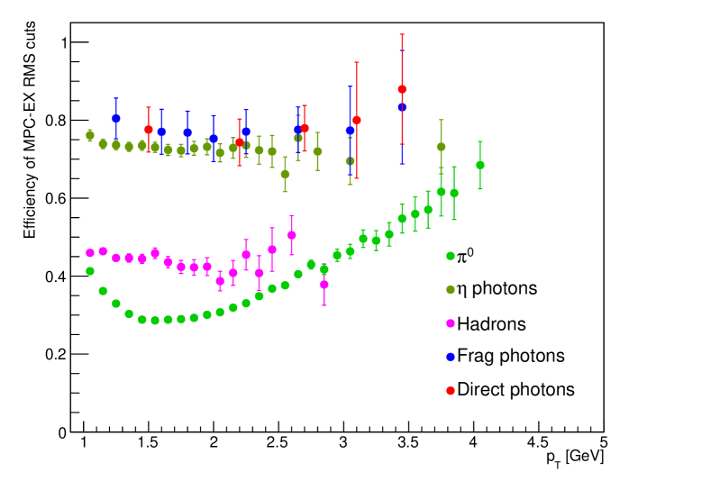
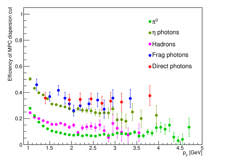
Figure 3.48: The efficiency of the MPC-EX RMS and MPC dispersion cuts as a function of $p_{T}$. The right panel shows the efficiency for the MPC-EX RMS cut and the left panel the MPC dispersion. $\pi^{0}$ and $\eta$ decays are shown in bright and olive green respectively. Hadrons are shown in pink. Direct photons are shown in red and fragmentation photons in dark blue.

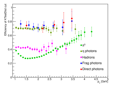
Figure 3.49: The efficiency of the KTestDist cut as a function of $p_{T}$. $\pi^{0}$ and $\eta$ decays are shown in bright and olive green respectively. Hadrons are shown in pink. Direct photons are shown in red and fragmentation photons in dark blue.

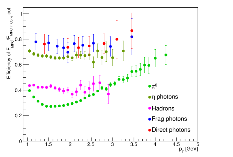
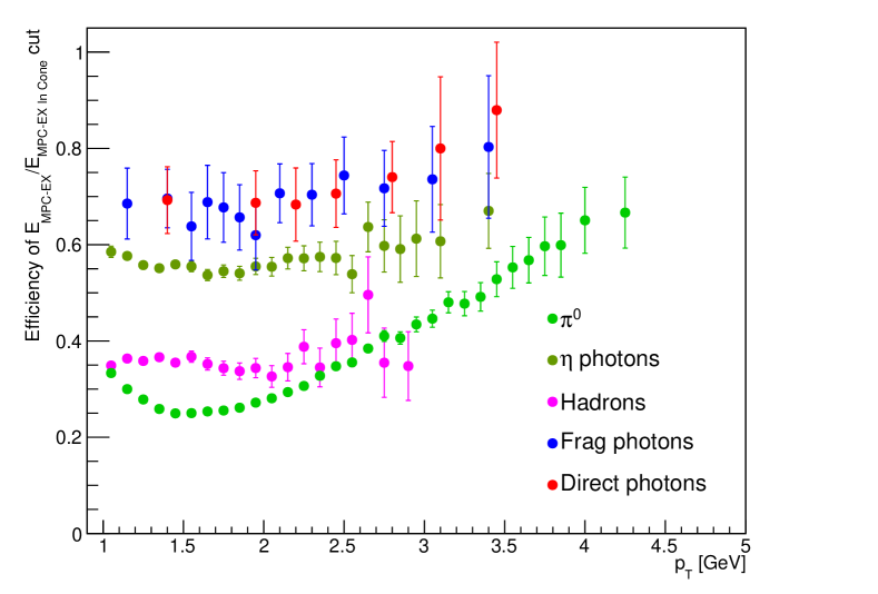
Figure 3.50: The efficiency of the energy ratio in cone cuts considering the energies in the MPC and MPC-EX as a function of $p_{T}$. The right panel shows the efficiency using the MPC energies and the left panel shows the ratio with MPC-EX energies. $\pi^{0}$ and $\eta$ decays are shown in bright and olive green respectively. Hadrons are shown in pink. Direct photons are in red and fragmentation photons in dark blue.

Table 3.7 presents the yields and efficiencies for all particle types in this analysis. Figure 3.51 shows the efficiency distribution of the photon candidates as a function of $p_{T}$. Direct photons are the most efficient particle type, with an efficiency of $31.2\%$ at a $p_{T}$ above 3 GeV. Fragmentation photons have a slightly lower efficiency of $23.2\%$ at high $p_{T}$. Hadrons and $\pi^{0}$ background efficiencies are $5.1\%$ and $2.8\%$ respectively. These cuts separate hadrons and $\pi^{0}$ backgrounds from the direct photon signal.

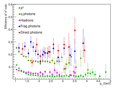
Figure 3.51: The efficiency of the photon candidate cuts as a function of $p_{T}$. $\pi^{0}$ and $\eta$ are shown in bright and olive green. Hadrons are shown in pink. Direct photons are in red and fragmentation photons in dark blue.

Table 3.7: Particle yields and efficiencies with all of the cuts in Table 3.5 applied.

Particle Type	Yield	Efficiency
Charged hadrons	6	6.1$\%$
$\pi$	5	11.4$\%$
K	0	0.0$\%$
p	0	0.0$\%$
neutrons	0	0.0$\%$
other	1	1.9$\%$
$\pi^{0}$	234	2.9$\%$
$\eta$ decay	51	11.5$\%$
Other decays	11	9.6$\%$
$\omega$	9	9.6$\%$
$\eta$’	1	5.3$\%$
other	1	100.0$\%$
Signal photons	101	27.8$\%$
frag photons	43	24.3$\%$
direct photons	58	31.2$\%$

Fragmentation photons

While fragmentation photons are included in NLO calculations within the MPC-EX acceptance, PHENIX measurements of fragmentation photons [8] indicate that fragmentation photons are not a significant fraction of the signal photon yield at midrapidity. Despite the uncertainty in the expected levels of fragmentation photon production, we design cuts to increase the relative contribution of direct photons to the signal and reduce the fragmentation photons. This allows the direct photon measurement to more easily access the gluon contribution to the measured photon signal since fragmentation photons lower the sensitivity of the signal photon $R_{dA}$, as seen in Section 1.1. In this section, we consider our ability to separate fragmentation and direct photons with the MPC-EX detector.

For the direct photon measurement, both the fragmentation and direct photons are measured as signal. The analysis in Section 3.2.8 focuses primarily on removing the $\pi^{0}$ background and results in 101 signal photons, 58 of which are direct photons. A direct photon concentration of 57.4%. This is an increase from the roughly equal contribution of fragmentation and direct photons before the $\pi^{0}$ rejection cuts are applied. The contribution from fragmentation photons is reduced even further by tightening the MPC and MPC-EX variables introduced in Section 3.2.8 and using new variables to differentiate between fragmentation and direct photons. Here we present two additional analyses to highlight our ability to remove fragmentation photons.

Direct photons are produced with no neighboring particles while fragmentation photons are within a jet of correlated particles. Isolation variables, such as the number of tracks within a cone around the candidate track and the ratio of the track’s energy to the amount of energy deposited in a cone around the track, are able remove fragmentation photons. These isolation variables are designed to reject fragmentation photons, but they can also reduce $\pi^{0}$ and hadrons from jets. The energy ratio in cone variables, $E_{MPC-EX}/E_{MPC-EXInCone}$ and $E_{MPC}/E_{MPCInCone}$, shown in Figure 3.45, successfully reduce $\pi^{0}$ and hadrons with the cuts presented in Section 3.2.8. By tightening these energy ratios, fragmentation photons can also be removed from the sample.

The number of electromagnetic tracks (NumInCone) and hadron-like tracks (HadInCone) in a one radius cone in $\eta$-$\phi$ space around the photon candidate track are additional measures of the candidate track’s isolation. The hadron-like tracks used in HadInCone are defined by requiring narrow MIP deposits in all layers of the MPC-EX with poor non-unique matching to the MPC. The electromagnetic tracks are only required to have a unique match to an MPC cluster. The NumInCone variable has a minimum value of one since the cone contains the photon candidate track. Figure 3.52 shows the NumInCone and HadInCone distributions for $\pi^{0}$, hadrons and direct and fragmentation photons. Both the NumInCone and HadInCone distributions are largest at their minimum values with the yields falling steeply as the value increases. At the lowest values for each variable, the direct photon yields to the fragmentation photon contribution. At higher values of NumInCone a small separation can be seen with the direct photon yield lower than the fragmentation photon yield.

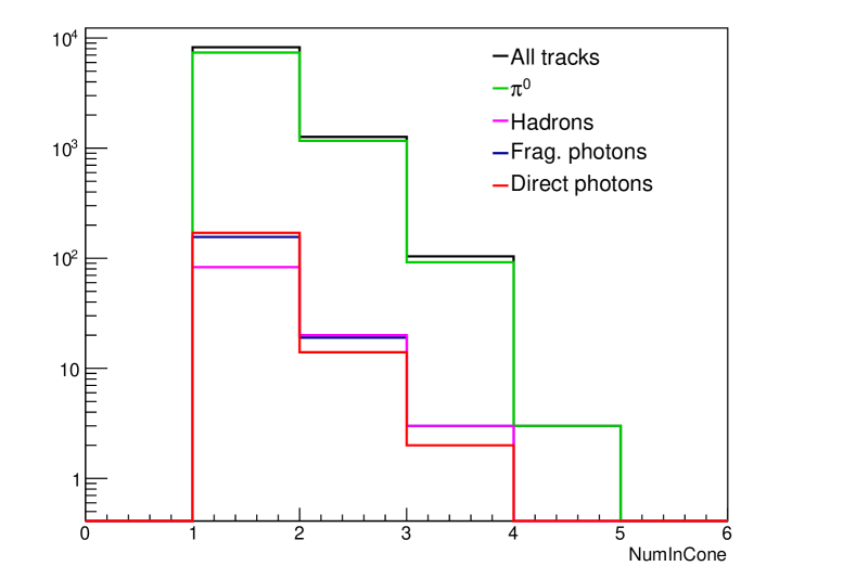
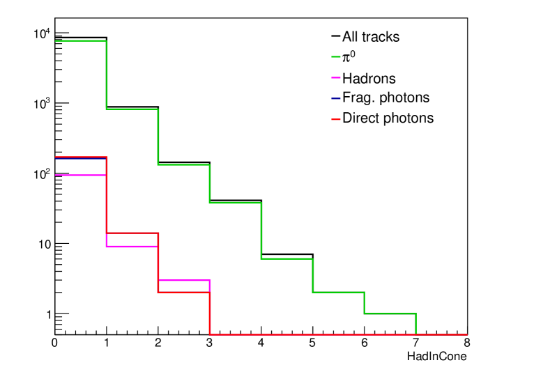
Figure 3.52: The NumInCone and HadInCone distributions are shown on the left and right respectively. Pions are shown in green and hadrons are shown in pink. The direct photon are shown in red and fragmentation photons are in blue. The sum of all tracks is shown in black.

Isolated tracks are defined as tracks where NumInCone is one and HadInCone is zero. The efficiencies of these requirements is plotted in Figure 3.53. Unfortunately the HadInCone and NumInCone isolation cuts do not yet provide a substantial separation between direct and fragmentation photons on their own. Photons from $\eta$ decay are reduced by the NumInCone equal to one requirement, but the desired reduction of fragmentation photons is limited. At $p_{T}$ greater than 3 GeV, direct photons have an efficiency of 91.4% and fragmentation photons have an efficiency of 87.6%. Similar efficiencies for the HadInCone cuts are 91.4% and 91.0% for direct and fragmentation photons respectively. This limits our ability to remove the fragmentation photon contribution with these cuts alone. However, when these cut are applied in conjunction with other tightened cuts fragmentation photons are removed from the sample.

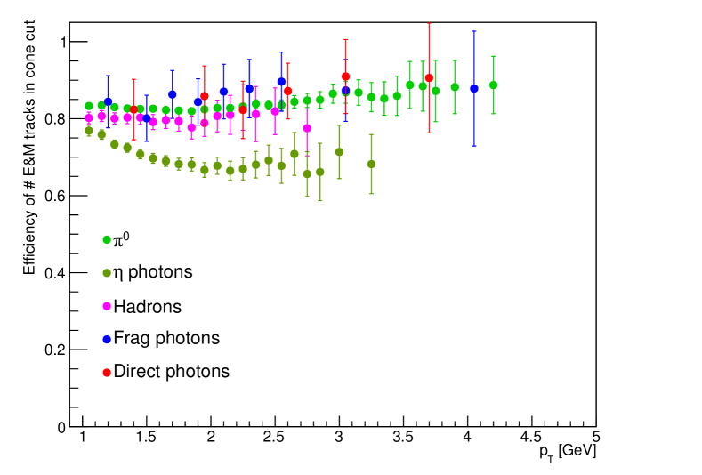
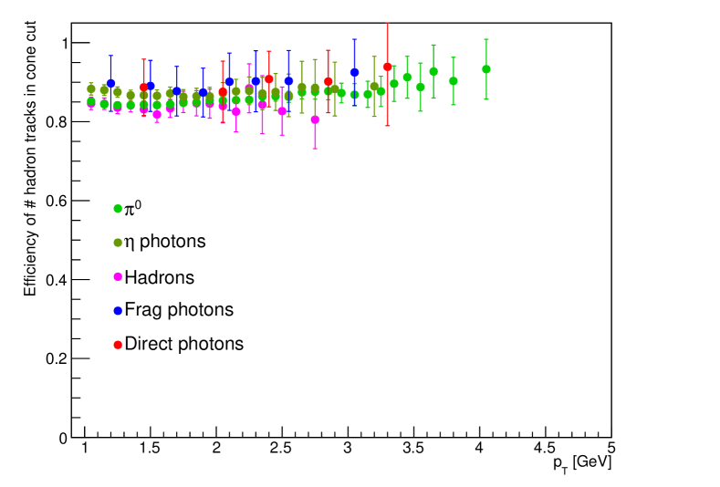
Figure 3.53: The efficiency of the track isolation cuts as a function of $p_{T}$. On the left, the NumInCone of one cut efficiency is shown and on the right the HadInCone of zero cut efficiency distributions is shown. $\pi^{0}$ and $\eta$ are shown in light and olive green. Hadrons are shown in pink. Direct photons are shown in red and fragmentation photons are in blue.

We also consider an additional variable, the ratio of the energy in the MPC-EX to the total energy from both the MPC and MPC-EX; this distribution is shown in Figure 3.54. A shape difference in the direct photon distribution compared to the $\pi^{0}$ is seen. Like many of the distributions shown previously, it is difficult to identify a difference in the direct and fragmentation photon distributions with the low statistics available in the $p_{T}>3$ region.

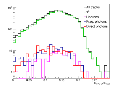
Figure 3.54: The ratio of the MPC-EX energy over the total energy in the MPC and MPC-EX as a function of $p_{T}$. Direct photon are shown in red and fragmentation photons are in blue. Hadron and $\pi^{0}$ tracks are in pink and green respectively. The sum of all tracks is shown in black.

To separate the direct photons from fragmentation photons a second TMVA analyses is completed. Direct photons are identified as the signal and fragmentation photons are the background. The TMVA sample is restricted to isolated tracks with $p_{T}$ above 3 GeV that pass the mass cut, the hadron cuts and the KTestDist cut from the Table 3.5. These cuts are applied to restrict the TMVA phase space to those tracks surviving the hadron and limited $\pi^{0}$ cuts detailed previously. The results from the CutsSA algorithm at two points on the ROC curve are considered. The first is located at a projected direct photon efficiency of 57% and a projected fragmentation photon rejection of 60.2%; this is refered to Frag Cuts 1. The second is located at a projected direct photon efficiency of 47% and a projected fragmentation photon rejection of 78.9%; this is referred to Frag Cuts 2. Both of these cuts are listed in Table 3.8.

Table 3.8: Acceptable ranges for variables as defined by TMVA to remove fragmentation photons.

Variable	Frag Cuts 1	Frag Cuts 2
$E_{MPC-EX}/E_{Total}$	0.034 - 0.214	0.017 - 0.172
dispersion	1.154 - 2.645	1.530 - 2.544
RMS	3.075 - 6.847	2.479 - 8.242
KTestDist	0.153 - 0.378	0.115 - 0.385
$E_{MPC-EX}/E_{MPC-EXInCone}$	$>$ 0.868	$>$ 0.869
$E_{MPC}/E_{MPCInCone}$	0.832 - 1.021	0.793 - 0.960

A comparsion of the acceptable variable ranges between Frag Cuts 1 and Frag Cuts 2 shows that the minimum on the dispersion and the maximum on the RMS are increased as the fragmentation photon rejection rises. The $E_{MPC-EX}/E_{Total}$ and KTestDist variables are lowered and the maximum on the $E_{MPC}/E_{MPCInCone}$ is reduced. The $E_{MPC-EX}/E_{MPC-EXInCone}$ range is unaffected. Comparison of the cuts in Table 3.8 and those in Table 3.5 shows that the RMS and dispersion variables are similarly constrained but with an lower ranges than seen in the $\pi^{0}$ cuts. The energy in cone ratios and KTestDist are more tightly restricted when removing fragmentation photons. The $\pi^{0}$ and fragmentation photon rejection cut sets are combined so that the intersection of the cut regions are applied. By retaining only the overlap of the allowable variable ranges background removal is maximized. The downside to this is that the efficiency of the direct photons are reduced. The combined cuts are listed in Table 3.9 and Cuts 1 efficiencies are listed in Table 3.10.

Table 3.9: Acceptable ranges for variables as defined by TMVA to remove both $\pi^{0}$ and fragmentation photons.

Variable	Cuts 1	Cuts 2
$E_{MPC-EX}/E_{Total}$	0.034 - 0.214	0.017 - 0.172
dispersion	1.154 - 1.631	1.530 - 1.631
RMS	3.075 - 6.118	2.479 - 6.118
KTestDist	0.153 - 0.378	0.115 - 0.385
$E_{MPC-EX}/E_{MPC-EXInCone}$	$>$ 0.868	$>$ 0.869
$E_{MPC}/E_{MPCInCone}$	0.832 - 1.013	0.793 - 0.960

Table 3.10: Efficiencies using the Cuts 1 ranges in Table 3.9 for $\pi^{0}$, hadrons, direct and fragmentation photons for yields at $p_{T}>3$ GeV.

Variable	$\epsilon_{\pi^{0}}$	$\epsilon_{hadrons}$	$\epsilon_{\gamma frag}$	$\epsilon_{\gamma direct}$
Mass	$29.1\%$	$37.5\%$	$84.2\%$	$90.3\%$
$E_{MPC-EX}/E_{Total}$	$48.6\%$	$45.2\%$	$62.2\%$	$73.1\%$
dispersion	$8.4\%$	$7.7\%$	$34.5\%$	$34.4\%$
RMS	$50.2\%$	$47.1\%$	$66.1\%$	$74.7\%$
KTestDist	$33.6\%$	$35.6\%$	$39.5\%$	$54.8\%$
$E_{MPC-EX}/E_{MPC-EXInCone}$	$45.9\%$	$44.2\%$	$58.2\%$	$68.3\%$
$E_{MPC}/E_{MPCInCone}$	$44.7\%$	$37.5\%$	$59.3\%$	$71.0\%$
NumInCone	$86.7\%$	$78.8\%$	$87.6\%$	$91.4\%$
HadInCone	$88.6\%$	$89.4\%$	$91.0\%$	$91.4\%$
All Cuts 1 applied	$1.4\%$	$1.0\%$	$7.3\%$	$15.1\%$

The hadrons and $\pi^{0}$ backgrounds are rejected by the mass, $E_{MPC-EX}/E_{Total}$, dispersion, KTestDist, and energy ratio in cone variables with $\pi^{0}$ efficiencies of less than $50\%$. The $E_{MPC-EX}/E_{Total}$, KTestDist and energy ratio in cone variables also distinguish between fragmentation and direct photons with a separation in direct and fragmentation photons efficiencies of more than 10%. Figures 3.55,  3.56 and 3.57 show the efficiencies as a function of $p_{T}$ for the variables: dispersion, RMS, $E_{MPC-EX}/E_{Total}$, KTestDist, and the energy in cone ratios with the Cuts 1 ranges. Comparing the Cut 1 efficiencies with the RMS, dispersion, KTestDist and energy ratio in cone variables with the $\pi^{0}$ cut efficiencies in Figures 3.48, 3.49 and 3.50 shows an overall decrease in the cut efficiencies except for the dispersion cut and a minimal affect seen in KTestDist.

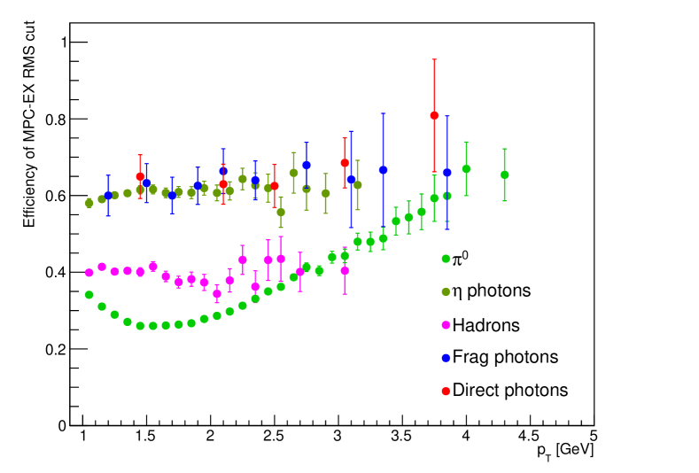
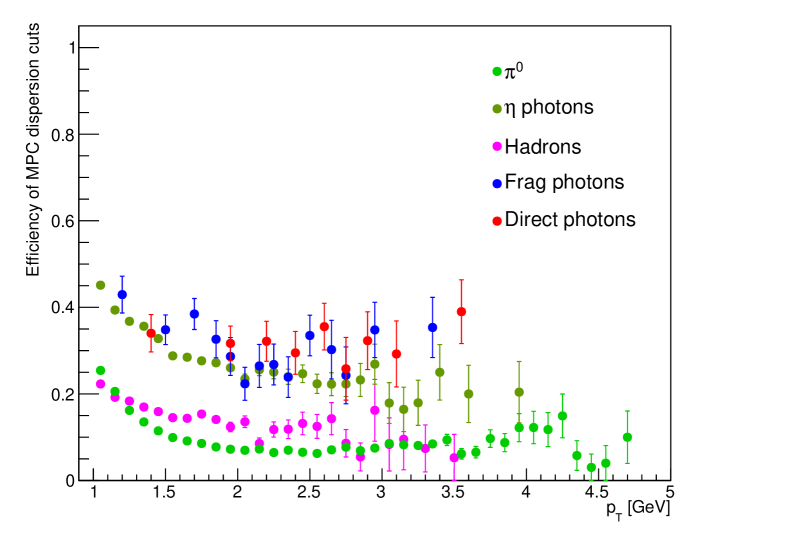
Figure 3.55: The efficiency of the MPC-EX RMS and the MPC dispersion cuts in the Cuts 1 range as a function of $p_{T}$. The right panel shows the MPC-EX RMS cut efficiency and the left panel shows the efficiency of the MPC dispersion cut. $\pi^{0}$ and $\eta$ are shown in bright and olive green. Hadrons are shown in pink. Direct photons are shown in red and fragmentation photons in blue.

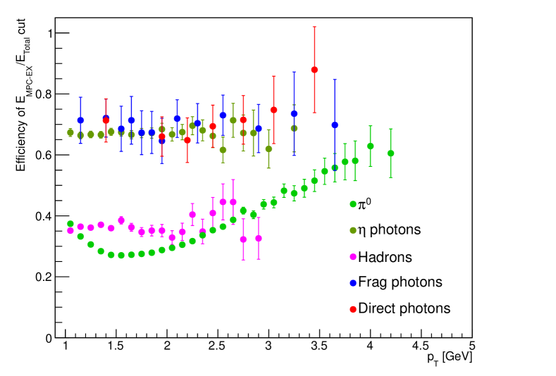
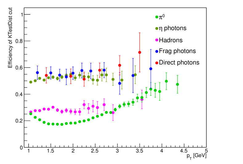
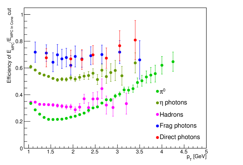
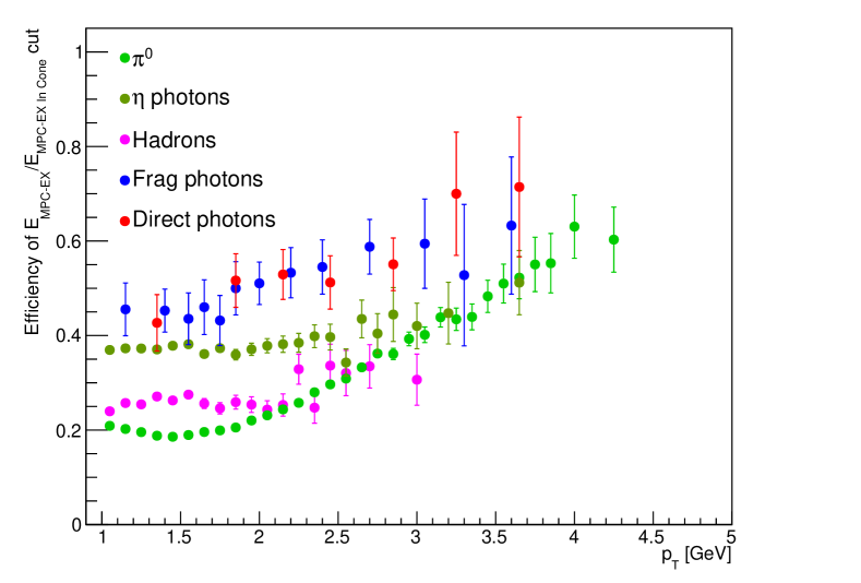
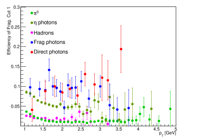
Figure 3.56: The efficiency of the $E_{MPC-EX}/E_{Total}$ and KTestDist cuts in the Cuts 1 range as a function of $p_{T}$. The right panel shows the $E_{MPC-EX}/E_{Total}$ cut efficiency and the left panel shows the efficiency of the KTestDist cut. $\pi^{0}$ and $\eta$ are shown in bright and olive green. Hadrons are shown in pink. Direct photons are shown in red and fragmentation photons in blue.

Figure 3.57: The efficiency of the energy ratio in cone cuts considering the energies in the MPC and MPC-EX as a function of $p_{T}$. The right panel shows the efficiency using the MPC energies and the left panel shows the ratio with MPC-EX energies. $\pi^{0}$ and $\eta$ decays are shown in bright and olive green. Hadrons are shown in pink. Direct photons are shown in red and fragmentation photons in blue.

Figure 3.58: The total efficiency of the Cuts 1 ranges as a function of $p_{T}$. Direct photon are shown in red and fragmentation photons are in blue. Hadrons, $\pi^{0}$ and $\eta$ are in pink, light and olive green respectively.

Comparing the efficiencies in Tables 3.6 and 3.10 confirms that the RMS, KTestDist and energy in cone ratio cuts show a lower direct photon efficiency and an increased separation between the direct and fragmentation photon efficiencies; the $\pi^{0}$ efficiencies remain roughly the same. The mass cut and resulting efficiencies are unchanged in both cases. The dispersion efficiencies are only minimally effected despite the reduced range. This is because the dispersion distribution is sparingly populated below 1.154.

As expected, the efficiencies in the Cuts 1 analysis are reduced compared to the $\pi^{0}$ cuts analysis. Figure 3.58 shows the efficiency in the Cuts 1 analysis as a function of $p_{T}$. A comparison to Figure 3.51 shows an increased separation between the direct and fragmentation photons at high $p_{T}$. Table 3.11 shows the yields for the $\pi^{0}$, Cuts 1 and Cuts 2 analyses and when only the hadron cuts are applied. The resulting $\pi^{0}$ and direct photons efficiencies and yields in the Cuts 1 case are approximately half, 48%, of the $\pi^{0}$ cuts case. Fragmentation photons are down by roughly a third, 30%. The Cuts 2 analysis reduces the direct photons and $\pi^{0}$’s by 19% and 15% compared to the $\pi^{0}$ rejection analysis; fragmentation photons are reduced by 7%. By tightening cuts and ensuring tracks are isolated we can increase the direct photon concentration while maintaining or increasing the direct photon-to-$\pi^{0}$ ratio.

Table 3.11: Particle yields with and with out various photon cuts.

Particle Type	Yield with	Yield with	Yield with	Yield with
	hadron cuts	$\pi^{0}$ cuts	Cuts 1	Cuts 2
Charged hadrons	99	6	1	0
$\pi$	44	5	1	0
K	0	0	0	0
p	0	0	0	0
neutrons	2	0	0	0
other	53	1	0	0
$\pi^{0}$	8013	234	112	35
$\eta$ decay	445	51	16	8
Other decays	114	11	4	2
$\omega$	94	9	4	2
$\eta$’	19	1	0	0
other	1	1	0	0
Signal photons	363	101	41	14
frag photons	177	43	13	3
direct photons	186	58	28	11

Before the $\pi^{0}$ cuts are applied, direct and fragmentation photons have a roughly equal contribution to the signal photons in the Pythia sample. After applying the $\pi^{0}$ cuts, direct photons are 57.4% of the signal photons. With the Cuts 1 analysis, the relative contribution of direct photons to the signal photon measurement increases to 68.3%. By applying the tighter Cuts 2 cuts, the relative contribution of the direct photons to 78.6% of the signal photons. These results show that with a MPC-EX detector we are able to adjust the concentration of direct photons in the measured signal.

In Section 3.4 the direct photon measurement using the double ratio method is discussed using the results from the $\pi^{0}$ cuts analysis. The measurements and the corresponding systematics for the Cuts 1 and Cuts 2 analyses with the increased relative direct photon contribution are also discussed for comparison.

3.3 Direct Photons in the Pythia Monte Carlo

A Pythia Monte Carlo is used to benchmark the MPC-EX’s ability to measure direct photons[56]. While Pythia is a simulation of p+p events, it serves as a good proxy for d+Au collisions in the deuteron-going direction. Pythia is well tuned to measured cross sections at the Tevatron and fixed-target energies. Studies with the event generator HIJING indicate that the additional multiplicity in a d+Au collision is localized at low energies, below the high energy direct photons emitted in the forward direction.

In addition to the Monte Carlo generator Pythia, the MPC-EX collaboration also solicited NLO calculations of the direct photon cross section from Werner Vogelsang for p+p collisions at 200 GeV [60]. A comparison between the NLO calculations and Pythia is shown in Figure 3.59. The NLO cross sections identify two photon sources: photons from partonic processes and QED radiation from incoming partons, which we refer to as “direct” photons, and photons from parton fragmentation, which we refer to as “fragmentation” photons. In the NLO calculation it is not possible to cleanly separate direct photons into their partonic and QED radiated components because the cross section calculation involves interference between different amplitudes. The Pythia Monte Carlo calculates partonic processes at leading order (LO) and QED radiated photons from incoming quarks are implemented in a separate process. In Pythia these two different sources of photons can be distinguished.

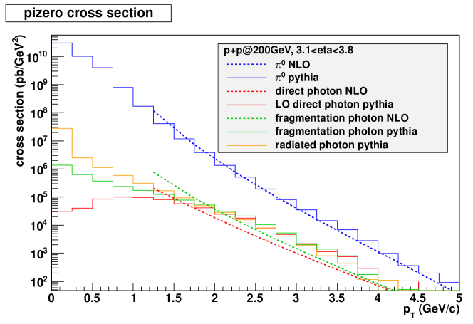
Figure 3.59: NLO cross sections fom Werner Vogelsang compared the cross sections extracted from Pythia for $\pi^{0}$’s and direct photons. Direct photons from Pythia are selected only from processes that produce a photon at the hard scattering vertex, fragmentation photons and QED radiation from incoming quarks are shown as separate entries.

Before proceeding to use Pythia to evaluate the performance of the MPC-EX, it is important to understand if Pythia properly reproduces the expected cross sections for direct and fragmentation photons, and $\pi^{0}$ mesons (the dominant background). In Figure 3.59, we compare the NLO cross sections for direct and fragmentation photons in the MPC-EX acceptance with the cross sections from the Pythia Monte Carlo model. A comparison of the $\pi^{0}$ cross section is also included. The $\pi^{0}$ cross sections are a very good match between Pythia and the NLO calculations. The fragmentation photon cross section is similar between the Pythia and NLO calculations, agreeing to within a factor of approximately two. The LO photons in Pythia are a good comparion in overall magnitude to the NLO direct photon cross sections (again, within roughly a factor of two). However, this is not an apples-to-apples comparison. The Pythia calculation is LO and does not include QED radiation from quarks incoming to the hard scattering vertex, while the NLO calculation includes this radiation and additional amplitudes. The cross section in Pythia for photons from QED radiation is comparable to the Pythia LO cross section. If the photons from incoming quark radiation are included in the MPC-EX analysis, the effective cross section will be much larger than the NLO cross section, potentially overestimating the sensitivity of the measurement.

Due to the nature of the NLO calculation, we cannot directly compare the QED radiated components between the NLO and Pythia calculations. However, in the MPC-EX acceptance the hard-scattering contribution to the direct photon cross section is dominated by gluon Compton scattering, which samples the gluon distribution in the Au nucleus. The ability to access the Au nuclei’s gluon distribution is the focus of the direct photon measurement. The portion of the cross section resulting from QED radiation samples the quark and antiquark parton distribution functions. These PDFs access a different region in Bjorken x. The NLO cross sections can be calculated as differential quantities in the parton $x_{2}$ by parton flavor to estimate the relative effect of direct photons from the hard scattering vertex (dominated by gluons) or from QED radiation from incoming quarks (dominated by the quark PDF’s). These differential cross sections are plotted in Figure 3.60, which shows that interactions involving the gluon in the target nucleon dominate the direct photon cross section by a large factor. Interactions involving quarks and antiquarks are substantially smaller, and result from interactions that produce direct photons (via processes other than gluon Compton) and proceses that produce direct photons by QED radiation from the incoming quarks.

(a)

(b)

(c)

(d)

(e)

(f)

Figure 3.60: Differential NLO cross sections fom Werner Vogelsang as a function of $x_{2}$ for gluons (a), u-quarks (b), d-quarks (c), anti-up quarks (d), anti-down quarks (e) and the combination of strange and anti-strange quarks (f). The vertical axis is $d\sigma/d\log(x_{2})$ in the pseudorapidity range $3.1<\eta<3.8$.

From the NLO differential cross sections in Figure 3.60, we conclude that the contribution of direct photons from QED radiation is small in the NLO calculation, and the Pythia Monte Carlo dramatically overestimates the contribution of these photons. Based on this, we exclude Pythia events from our analysis when direct photons are generated by this process. The remaining Pythia yield of LO direct and fragmentation photons, as well as the relative yield of these photons to $\pi^{0}$ mesons, more closely approximates the NLO calculations.

3.4 Direct Photons in d+Au Collisions

The direct photon can be measured with the MPC-EX detector at $p_{T}>3$ GeV. When the simulation is scaled up to the expected event rates, the $R_{dAu}$ measurement for signal photons at $p_{T}>3$ GeV is statistically precise. The measured $R_{dA}$’s ability to constrain existing models of the gluon nuclear parton distribution function depends on the systematic errors on the $R_{dAu}$ ratio.

At $p_{T}>3$ GeV, $\pi^{0}$ and $\eta$ decays are the primary backgrounds after applying the photon identification cuts. Signal photons are extracted from the $\pi^{0}$ and $\eta$ backgrounds using the double ratio method. First the simulation and the resulting signal photon and background yields are presented. Then the double ratio method and the corresponding systematic errors are discussed. Finally these values are used to demonstrate the sensitivity available with the MPC-EX detector to restrict the viable region of the EPS09 gluon modification distribution[35].

3.4.1 Simulation yields

The MPC-EX detector’s ability to measure direct photons in d+Au collisions is determined using a minimum bias 200 GeV p+p Pythia simulation with a realistic vertex distribution. At high transverse momenta, where the direct photon measurement is performed, binary-scaled p+p events provide a good approximation of d+Au events. Of the approximately 868 million simulated events, 270 million events satisfy the trigger requirement of a track with a MPC-EX energy above 16.5 GeV.

Table 3.12: Projected direct photon candidate yields in 49 $pb^{-1}$ p+p (12 weeks) and 0.35 $pb^{-1}$ d+Au (12 weeks) collisions using the Table 3.5 photon identification cuts.

Candidate Sources	p+p	d+Au
Hadrons	14293.6	847.4
$\pi$	11911.3	706.2
K	0.0	0.0
p	0.0	0.0
neutrons	0.0	0.0
other	2382.3	141.2
$\pi^{0}$	557448.4	33048.7
$\eta$ decay	121495.2	7202.9
Other hadron decays	26204.8	1553.6
$\omega$	21440.3	1271.1
$\eta$’	2382.3	141.2
other	2382.3	141.2
Signal photons	240608.1	14264.6
frag. photons	102437.1	6073.1
direct photons	138171.0	8191.6

The direct photon analysis yields using the Pythia simulation is adjusted to give the total expected yields in p+p and d+Au collisions. Table 3.12 presents the projected yields assuming a total integrated luminosity of 49 $pb^{-1}$ in 12 weeks of $\sqrt{200}$ GeV p+p collisions and 0.35 $pb^{-1}$ in 12 weeks of $\sqrt{200}$ GeV d+Au collisions. These luminosities are calculated in Appendix J. The simulated results using the $\pi^{0}$ rejection cuts from Table 3.5 in Section 3.2.8 are used in this projection. With these projected yields the $R_{dAu}$ measurement is statisically precise with a relative statistical error of approximatly 1.16%. The significance of the signal photon $R_{dA}$ measurement hinges on the systematic errors discussed later in this section.

Signal photon candidates are selected with the $\pi^{0}$ rejection cuts described in Table 3.5 in Section 3.2.8. Figure 3.61 presents the $p_{T}$ distributions for the direct photons and backgrounds surviving these cuts. $\pi^{0}$ and photons from $\eta$ decays are the largest remaining components. The direct photon signal remains below the $\pi^{0}$ contribution at all $p_{T}$ values. At $p_{T}$ greater than 3 GeV, the direct photons yield is larger than the background photons from $\eta$ decays. Hadrons and other decay photons are relevant at lower $p_{T}$’s but are negligible compared to the direct photon contributions in the high $p_{T}$ range. Table 3.13 lists the particle contributions in four $p_{T}$ ranges with varied lower limits between 2.5 and 4 GeV. The direct photon candidates are separated into two $\eta$ ranges, an inner range of $3.1<\eta<3.45$ and an outer range of $3.45<\eta<3.8$, in Figure 3.62 and Table 3.14.

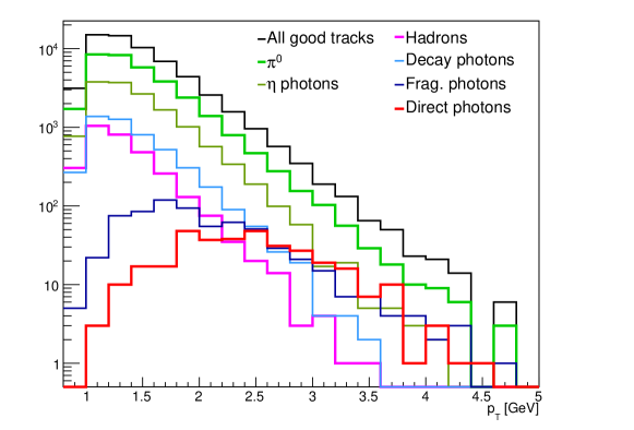
Figure 3.61: The $p_{T}$ distribution of photon candidate tracks. All of the photon candidate tracks are shown in black. The spectrum of photon candidates from $\pi^{0}$ (bright green) and $\eta$ (olive green) decays are shown separately. Remaining decays, primarily from $\omega$ and $\eta$’, are in light blue. Signal photons including those produced by fragmentation and the initial hard interactions are in blue and red respectively. Hadrons are in pink.

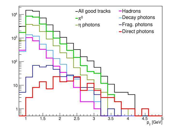
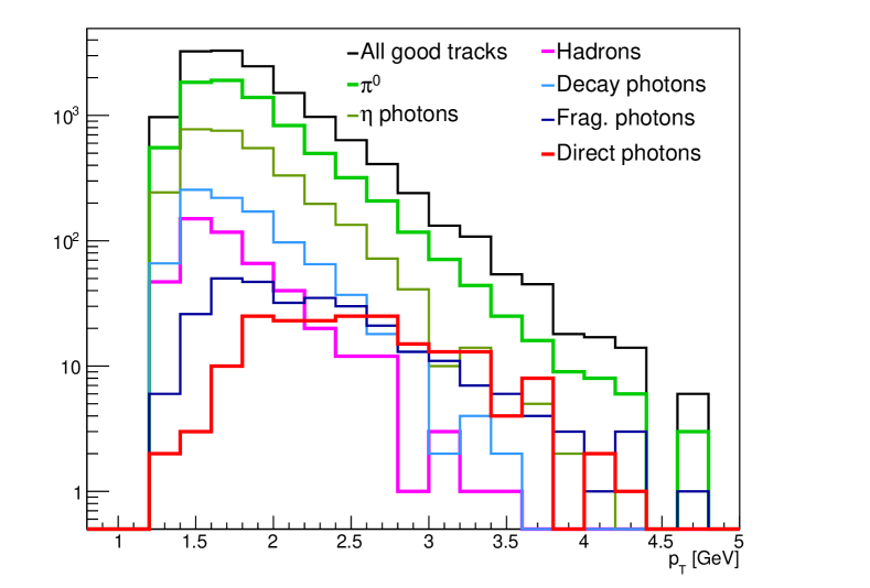
Figure 3.62: The $p_{T}$ distribution of photon candidate tracks in inner and outer $\eta$ ranges. The right panel shows the $p_{T}$ distribution with $\eta$ between 3.1 and 3.45. The left panel shows the $\eta$ distribution with $\eta$ between 3.45 and 3.8. All of the photon candidate tracks are shown in black, the spectrum of photon candidates from $\pi^{0}$ and $\eta$ decay are shown in bright and olive green. Direct photons from the initial hard interaction are shown in red and fragmentation photons are in dark blue. The direct and fragmentation photons are further broken down according to their interaction type, $q+q$, $q+\bar{q}$, $q+g$ and $g+g$ with various linestyles.

Signal photons are separated into direct photons from the initial hard scattering and photons from outgoing quark fragmentation. They are further divided by their initial hard production mechanisms. Direct photons from the initial hard scattering are produced by quark-gluon Compton scattering, quark-antiquark annihilation and gluon fusion. Fragmentation photons are produced in the following initial hard processes:

• $q+q\rightarrow q+q$

• $q+\bar{q}\rightarrow q+\bar{q}$ and $q+\bar{q}\rightarrow g+g$

• $q+g\rightarrow q+g$

• $g+g\rightarrow q+\bar{q}$ and $g+g\rightarrow g+g$

Direct photons from the initial hard scattering are divided into $q+\bar{q}$, $q+g$ and $g+g$ interaction types. Fragmentation photons are separated into $q+q$, $q+\bar{q}$, $q+g$ and $g+g$ interaction types. Figure 3.63 presents the $p_{T}$ distributions for the signal photon contributions, direct photons (red) and fragmentation photons (dark blue). The signal photon contributions are further separated by their hard interaction type, $q+q$ (dash-dot-dotted), $q+\bar{q}$ (dashed), $q+g$ (dotted) and $g+g$ (dash-dotted). The signal photon components separated by their hard interaction types are also detailed in Tables 3.13 and 3.14. Both the fragmentation photons and direct photons are dominated by the $q+g$ interaction. $q+\bar{q}$ interactions provide small contributions to fragmentation photons. There are no remaining $q+q$ or $g+g$ interactions.

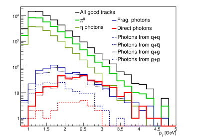
Figure 3.63: The $p_{T}$ distribution of the surviving signal photons separated by interaction type. All of the photon candidate tracks are shown in black. Direct photons from the initial hard interaction are shown in red and fragmentation photons are in dark blue. The signal photons are separated according to their interaction type, $q+q$, $q+\bar{q}$, $q+g$ and $g+g$ with the various linestyles, dashed-dot, dashed, dotted, and dash-dot-dot.

Table 3.13: Breakdown of direct photon candidates with various minimum $p_{T}$’s

Candidate Sources	$p_{T}>2.5$	$p_{T}>3.0$	$p_{T}>3.5$	$p_{T}>4.0$
Charged hadrons	29	6	1	0
$\pi$	25	5	1	0
K	0	0	0	0
p	0	0	0	0
neutrons	1	0	0	0
other	3	1	0	0
$\pi^{0}$	857	234	57	18
$\eta$ decay	293	51	13	2
Other hadron decays	75	11	2	1
$\omega$	59	9	2	1
$\eta$’	15	1	0	0
other	1	1	0	0
Signal photons	261	101	36	11
frag. photons	117	43	17	6
$q+q$	0	0	0	0
$q+\bar{q}$	19	3	0	0
$q+g$	98	40	17	6
$g+g$	0	0	0	0
direct photons	144	58	19	5
$q+\bar{q}$	4	0	0	0
$q+g$	137	58	19	5
$g+g$	0	0	0	0

Table 3.14: Breakdown of direct photon candidates at $p_{T}>3$ GeV with various $\eta$ ranges

Candidate Sources	$3.1<|\eta|<3.8$	$3.1<|\eta|<3.45$	$3.45<|\eta|<3.8$
Hadrons	6	4	2
$\pi$	5	4	1
K	0	0	0
p	0	0	0
neutrons	0	0	0
other	1	1	0
$\pi^{0}$	234	182	52
$\eta$ decay	51	37	14
Other hadron decays	11	8	2
$\omega$	9	1	1
$\eta$’	1	1	1
other	1	0	0
Signal photons	101	77	24
frag. photons	43	36	7
$q+q$	0	0	0
$q+\bar{q}$	3	3	0
$q+g$	40	33	7
$g+g$	0	0	0
direct photons	58	41	17
$q+\bar{q}$	0	0	0
$q+g$	58	41	17
$g+g$	0	0	0

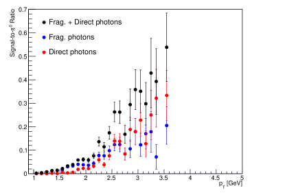
Figure 3.64: The signal-to-$\pi^{0}$ ratio versus $p_{T}$ for photon candidate tracks. The combined direct and fragmentation photon signal is shown in black. Fragmentation photons are in blue and direct photons are in red.

Figure 3.64 shows the signal-to-$\pi^{0}$ ratio as a function of $p_{T}$ for the photon candidates from fragmentation and direct photons using the $\pi^{0}$ rejection cuts. The signal-to-$\pi^{0}$ for the combined direct and fragmentation photon signal is shown and the ratios for the direct (red) and fragmentation (blue) photons are shown independently. As the $p_{T}$ increases, the signal-to-$\pi^{0}$ ratio also rises leading to a ratio of 0.43 $\pm$ 0.05 (stat) at $p_{T}$ greater than 3 GeV. Table 3.15 presents the signal-to-$\pi^{0}$ ratio for high $p_{T}$ signal photons with various photon identification cuts applied. The combined fragmentation and direct photon signal-to-$\pi^{0}$ ratio is unaffected by changing the $\eta$ range. The signal-to-$\pi^{0}$ ratios when the different cuts are applied ($\pi^{0}$ rejection vs. Cuts 1 vs. Cuts 2) are consistent with no effect on the ratio. This comparison is limited in by the large statistical errors in the simulation particularly for the Cuts 2 results. In Figure 3.64, the increase in the signal to background at high $p_{T}$ is in part a result of the decrease in the $\pi^{0}$ yields at high $p_{T}$ but it also reflects the fact that our $\pi^{0}$ rejection cuts are tailored to enhance the signal-to-$\pi^{0}$ ratio at high $p_{T}$. The direct photon signal-to-$\pi^{0}$ ratio increases at a steeper rate than then the fragmentation photon ratio. This shows the potential to increase the direct photon concentration in the measured signal at high $p_{T}$. The importance of the direct photon concentration and the ability to increase this quantity in the MPC-EX is presented in Sections 3.4.1 and 3.4.2.

Table 3.15: Signal-to-$\pi^{0}$ ratio of direct photon candidates with $p_{T}>3$ GeV and various cuts applied. The simulation’s statistical errors in these values are also presented.

Cuts used	Frag + direct	Frag.	Direct
$\pi^{0}$ rejection (Table 3.5),	0.43 $\pm$ 0.05	0.18 $\pm$ 0.03	0.25 $\pm$ 0.04
$3.1<|\eta|<3.8$
$\pi^{0}$ rejection (Table 3.5),	0.42 $\pm$ 0.06	0.20 $\pm$ 0.04	0.22 $\pm$ 0.04
$3.1<|\eta|<3.45$
$\pi^{0}$ rejection (Table 3.5),	0.46 $\pm$ 0.11	0.13 $\pm$ 0.05	0.33 $\pm$ 0.06
$3.45<|\eta|<3.8$
Cuts 1 frag. rejection (Table 3.9),	0.37 $\pm$ 0.07	0.12 $\pm$ 0.03	0.25 $\pm$ 0.05
$3.1<|\eta|<3.8$
Cuts 2 frag. rejection (Table 3.9),	0.40 $\pm$ 0.13	0.09 $\pm$ 0.05	0.31 $\pm$ 0.11
$3.1<|\eta|<3.8$

Remaining fragmentation photons

Direct photons are more strongly suppressed by the nuclei’s gluon distribution in a d+Au collision. Reducing the number of measured fragmentation photons and understanding their contribution to the signal photon measurement may increase the significance of the $R_{dA}$ measurement and thereby increase the EPS09 exclusion regions. The effect of some fragmentation photon contamination in the signal photon $R_{dA}$ is simulated and shown in Section 1.1.

Before photon identification cuts are applied, direct and fragmentation photons have roughly equal contributions to the signal photons in the Pythia sample. As mentioned in Section 3.2.8, the $\pi^{0}$ cuts increase the direct photon contribution to 57.4% of the signal photon measurement. With the less efficient Cuts 1 and Cuts 2 analyses, which are designed to reduce the fragmentation photon contribution, direct photons are 68.3 and 78.6% of the signal measurement respectively. These cuts are presented in Table 3.9 in Section 3.2.8. As a comparison two additional analyses are completed with these tighter fragmentation cuts, Cuts 1 and Cuts 2, applied. Figure 3.65 shows the $p_{T}$ distributions of the surviving photon candidate tracks from the Cuts 1 and Cuts 2 analyses. The photon candidate yields decrease considerably. The simulation yields with the Cuts 1 and Cuts 2 ranges applied are listed in Table 3.11 in the Section 3.2.8.

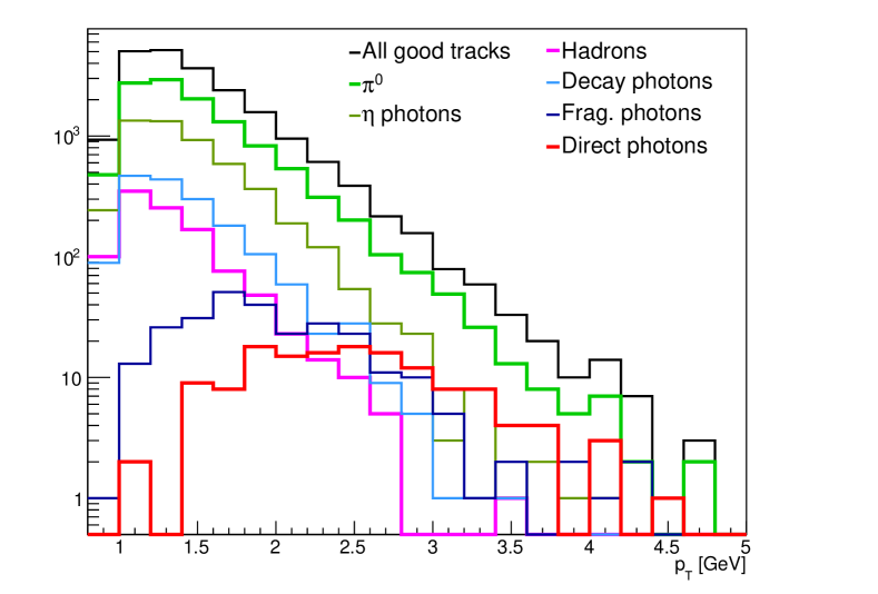
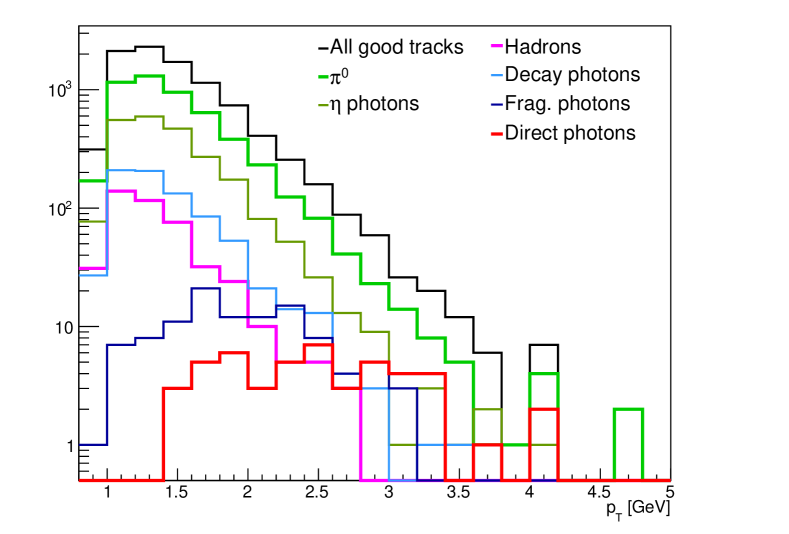
Figure 3.65: The $p_{T}$ distribution of photon candidate tracks using the Cuts 1 and Cuts 2 analyses presented in Section 3.2.8. The right panel shows the $p_{T}$ distribution with the Cuts 1 ranges applied. The left panel shows the $p_{T}$ distribution with the Cuts 2 ranges applied. All of the photon candidate tracks are shown in black, the spectrum of photon candidates from $\pi^{0}$ and $\eta$ decay are shown in bright and olive green. Other decays and hadrons are in light blue and pink respectively. Direct photons from the initial hard interaction are shown in red and fragmentation photons are in dark blue.

Table 3.16: Systematic errors of direct photon candidates in various $\eta$ ranges. For the final exclusion plots the full $\eta$ range is used.

	$3.1<|\eta|<3.8$	$3.1<|\eta|<3.45$	$3.45<|\eta|<3.8$
direct-to-signal ratio	57.4%	58.3%	56.6%
$\Delta\gamma_{Incl}/\gamma_{Incl}$	0.65%	0.85%	0.21%
Rγ	1.34	1.34	1.35
$\Delta$ Rγ/ Rγ	7.22%	7.24%	7.24%

Table 3.17: Systematic errors of direct photon candidates in various $p_{T}$ ranges. For the final exclusion plots the full $p_{T}>3.0$ GeV range is used.

	$p_{T}>2.5$	$p_{T}>3.0$	$p_{T}>3.5$	$p_{T}>4/0$
direct-to-signal ratio	43.7%	57.4%	52.8%	45.5%
$\Delta\gamma_{Incl}/\gamma_{Incl}$	0.85%	0.65%	0.93%	0.00%
Rγ	1.21	1.34	1.50	1.52
$\Delta$ Rγ/ Rγ	7.25%	7.22%	7.21%	7.21%

Table 3.18: Systematic errors of direct photon candidates with varied fragmentation photon contributions. For the final exclusion plots the $\pi^{0}$ cuts are used.

	$\pi^{0}$ Cuts	Cuts 1	Cuts 2
direct-to-signal ratio	57.4%	68.3%	78.6%
$\Delta\gamma_{Incl}/\gamma_{Incl}$	0.65%	0.46%	0.00%
Rγ	1.34	1.31	1.31
$\Delta$ Rγ/ Rγ	7.22%	7.22%	7.21%

3.4.2 Calculation of R_dAu and Systematic errors

The direct photon yield is calculated using a double ratio method that allows for the cancellation of many of the systematic errors. This method is used in many other analyses published by the PHENIX collaboration [10]. The ratio, R_γ, is calculated using the measured inclusive photon and $\pi^{0}$ spectra compared to the known contributions from hadronic decays relative to the $\pi^{0}$. Equation 3.1 presents the formula for R_γ,

$$R_{\gamma}=\frac{\left(\frac{\gamma_{Incl}}{\pi^{0}}\right)_{Meas}}{\left(\frac{\gamma_{Incl}}{\pi^{0}}\right)_{Sim}}$$ (3.1)

where $\gamma_{Incl}$ and $\pi^{0}$ are the inclusive photon and $\pi^{0}$ spectra respectively. The numerator is the measured inclusive photon-$\pi^{0}$ ratio and the denominator is a simulated ratio based on the known decay particle yields. Direct photons in the measured inclusive photon spectrum result in R_γ values greater than one. In turn the R_γ value is used to determine the direct photon contribution from the inclusive photon spectrum according to Equation 3.2.

$$\gamma_{Direct}=\gamma_{Incl}*\left(1-1/R_{\gamma}\right)$$ (3.2)

We estimate R_γ using our simulated analysis. First the hadron contributions are subtracted to determine the measured $\gamma_{Incl}$ spectrum. The simulated $\gamma_{Incl}^{sim}$ spectrum is approximated by summing the various photon decay contributions, $\gamma_{Incl}^{sim}=\pi^{0}+\eta+\eta^{\prime}+\omega+$other hadronic decays. The R_γ value is calculated from the yields in Table 3.14 producing an average value of 1.34 over the MPC-EX’s $\eta$ acceptance.

Based on the MPC-EX’s capabilities and the experience with the MPC[50], the $\pi^{0}$ cross-section at energies above 20 GeV can be measured to within an estimated systematic error of about 6%, including the effects of an uncertainty in the absolute energy scale of 1 to 2%. The error in $\gamma_{incl}$ is also dominated by the energy scale. The effects of these energy scale uncertainties in the final results are quantified later in this section. In the MPC analysis at low $p_{T}$ the main systematic uncertainty arose from the combinatorial background subtraction. This is not an issue for single-track analysis in the MPC-EX. The MPC-EX will be unable to provide detailed information on false photon candidates created by charged hadrons interacting in the detector. We expect that this background will be model dependent, and assign as 20% systematic error to this component. Finally there is an additional systematic error of 3% on $R_{dAu}$ from the determination of $\langle N_{coll}\rangle$ in the Glauber model (under the assumption that the systematic error in the p+p cross section cancels in the $R_{dAu}$ ratio)[51].

The systematic error in R_γ is calculated according to Equation 3.3

$$\Delta R_{\gamma}=\frac{\delta R_{\gamma}}{\delta\gamma_{Incl}}\Delta\gamma_{Incl}\oplus\frac{\delta R_{\gamma}}{\delta\pi^{0}}\Delta\pi^{0}\oplus\frac{\delta R_{\gamma}}{\delta MC_{sim}}\Delta MC_{sim}$$ (3.3)

where $MC_{sim}$ is the simulated inclusive photon-to-$\pi^{0}$ ratio. Equation 3.4 gives the relative systematic error of R_γ.

$$\frac{\Delta R_{\gamma}}{R_{\gamma}}=\frac{\Delta\gamma_{Incl}}{\gamma_{Incl}}\oplus\frac{\Delta\pi^{0}}{\pi^{0}}\oplus\frac{\Delta MC_{sim}}{MC_{sim}}$$ (3.4)

Tables 3.16, 3.17 and 3.18 present the systematic errors calculated for the R_γ assuming 6% relative error in the $\pi^{0}$ as mentioned previously, 4% relative error in the simulated $\gamma_{Inc}$-to-$\pi^{0}$ ratio, and 20% relative error in the hadron subtraction from the inclusive photons. Table 3.16 displays the R_γ and its systematic error for the $\pi^{0}$ rejection analysis over the entire MPC-EX $\eta$ acceptance and separated into inner and outer $\eta$ ranges. Table 3.17 presents the same information for various $p_{T}$ lower limits ranging from 2.5 to 4 GeV. In these tables, the R_γ appears to increase at higher $p_{T}$ and is unaffected by the separate $\eta$ ranges. The relative systematic error in R_γ remains stable at values around 7.22%. Table 3.18 is particularly valuable since it allows us to compare the R_γ and the corresponding systematic errors for various direct photon concentrations. The R_γ values are flat within the systematic errors and there is little to no improvedment in the R relative systematic error. However, the statistical errors in the Cuts 1 and Cuts2 analyses are larger as a result of the reduced yields and low signal efficiencies of these cuts as seen in Section 3.2.8. We continue with the preferred $\pi^{0}$ cuts analysis because of the larger signal efficiency and the lack of a substantial effect on R_γ as a result of the fragmentation photon contribution.

We now have R_γ, $\gamma_{incl}$ and their associated systematic errors for both p+p and d+Au. The statistical errors on the yields as input to the final result are calculated using Appendix J and the efficiencies given in Table 3.7. R_dAu is then calculated in each bin of $\eta$ as

$$R_{dAu}=\frac{1}{\langle N_{coll}\rangle}\frac{\gamma_{Incl}^{dAu}*\left(1-1/R_{\gamma}^{dAu}\right)}{\gamma_{Incl}^{pp}*\left(1-1/R_{\gamma}^{pp}\right)}$$ (3.5)

.

3.4.3 EPS09 Exclusion Plot

The MPC-EX’s ability to constrain the viable region of the EPS09 gluon modification, R_G, is presented as an exclusion plot. Here we detail how the exclusion plot is calculated and how the 1$\sigma$ and 90% confidence level bands are determined. The gluon suppression factor from EPS09 is assumed. Our simulated photon events are weighted according to their x₂ and Q² values and their sources, either direct photons, fragmentation photons, hadron decays or $\pi^{0}$ backgrounds. We then account for both statistical and systematic errors, and make an exclusion plot for the various R_G distributions given by EPS09[35]. We assume that the systematic error in R${}_{\gamma}^{pp}$ and R${}_{\gamma}^{dAu}$, which are dominated by the energy scale, are largely correlated. If the spectra p+p and d+Au spectra were identical, they would be completely correlated. To estimate the error from any difference between the p+p and d+Au spectra, a toy model of the raw spectra in p+p and d+Au is made. This gives the correct value of R_dAu for $\pi^{0}$s as measured in [50, 9]. The 2% energy scale error is propagated to R_γ. Figure 3.66 shows the ratio between the value of R_γ with a shifted energy scale to the R_γ without the energy scale shift. The error in R_γ is less than 1%. A similar procedure is followed to find the error in the ratio $\gamma_{inc}^{dAu}/\gamma_{inc}^{pp}$ resulting in an error value of 2%.

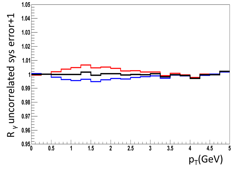
Figure 3.66: The ratio of R_γ in blue (red) where we have allowed the energy scale to be increased (decreased) by 2% over the nominal value. The black line is when no shift is applied and indicates the statistics of the simulation. The systematic error in $R_{\gamma}$ due to the energy scale less than 1%.

We vary all of the systematic errors over three standard deviations in each direction, a standard PHENIX procedure [6]. The systematic errors input into this calculation are summarized in Table 3.19. For each of the EPS09 R_G suppression functions we find the set of R${}_{\gamma}^{dAu}$, R${}_{\gamma}^{pp}$, $\gamma_{incl}^{dAu}$ and $\gamma_{incl}^{pp}$ values within three standard deviation of the nominal value located at the $\chi^{2}$ minimum. For each R_G curve, a value of the $\chi^{2}$ consistent with the simulated data is calculated. The associated $\chi^{2}$ values are used to identify the R_G curves that are within 1$\sigma$ of the simulated data. The R_G curves consistent at the 90% confidence level are also identified. The exclusion plots of R_dAu and the corresponding EPS09 suppression factors are shown in Figure 3.67. The hatched and light blue regions show the exclusion at the 90% confidence level for all of the EPS09 curves and using the simulated MPC-EX measurement respectively. The dark blue region represents the MPC-EX exclusion at the 1$\sigma$ limit. The black lines within the dark blue band are the EPS09 R_G curves that are consistent with the nominal values of the simulated data. The exclusion plots corresponding to Cuts 1 and 2 results are also calculated and are consistent with these results.

Table 3.19: Quantities used for the calculation of the exclusion plots.

Quantity	value	reference
Rγ	1.34	Table 3.18
systematic error $\Delta$ Rγ/ Rγ correlated between dAu and pp	7.2%	Table 3.18
systematic error $\Delta$ Rγ/ Rγ uncorrelated between dAu and pp	1%	Fig. 3.66
systematic error $\Delta\gamma_{Incl}/\gamma_{Incl}$ uncorrelated between dAu and pp	2%	from calculation similar to Fig. 3.66
relative systematic error on $\langle N_{coll}\rangle$	3%	[51]

Figure 3.67: EPS09 exclusion plots in R_dAu (left) and R_G (right). The outer hatched lines are the 90% confidence level envelope of all the EPS09 curves. The light blue areas represent the 90% confidence level limits of the simulated measurement, while the dark blue represent the 1$\sigma$ limits. The nominal value is taken as the central EPS09 curve.

The central value of EPS09 is taken as the nominal value in Figure 3.67. This is arbitrary. All values in the EPS09 range are equally probable and consistent with the world’s data. Figure 3.68 shows the excluded regions in two other cases where the upper and lower values are taken as the gluon suppression factor. In both of these instances, the viable region is reduced compared to the nominal EPS09 case. The exclusion region is particularly large when the lower value is used. Present PHENIX $\pi^{0}$ data shows a suppression at low-x indicating that lower values of EPS09 may be favored. However, this suppression could also be explained by the low $p_{T}$ of the measured $\pi^{0}$s. The MPC-EX direct photon measurement will clarify the effects of gluon suppression at low-x. It is important to note that EPS09 serves as the basis of comparison for this proposal. These exclusion plots illustrate the sensitivity of the MPC-EX direct photon measurement in a the context of a variety of theoretical pictures.

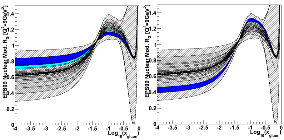
Figure 3.68: EPS09 exclusion plots in R_G where the nominal value is taken as the EPS09 curve corresponding to the least (left) or greatest (right) amount of suppression. The outer hatched lines are the 90% confidence level envelope of all the EPS09 curves. The light blue line represents the 90% confidence level limits of the simulated measurement, while the dark blue represent the 1$\sigma$ limits. No light blue region is visible if the 90% CL and the 1$\sigma$ level coincide to within the resolution given by the EPS09 theoretical curves available.

3.5 Direct Photon $A_{N}$

In a prompt (direct + fragmentation) photon measurement with the MPC-EX detector, the signal of prompt photons ($S$) and the background of hadron-decay photons ($B$) are mixed, with a signal to background ratio of $r=S/B$. For the MPC-EX, according to Monte Carlo simulations described in preceeding sections, with a cut of $p_{T}^{\gamma}>3$ GeV/c the value of $r$ typically is $\approx 0.4-0.5$. In measurements of a prompt photon SSA in 200 GeV spin polarized p+p collisions, the background photon events might carry a non-zero SSA, such as from $\pi^{0}$ or $\eta$ decay photons. The signal asymmetry ($A_{S}$) can be extracted from the measured asymmetry ($A_{meas}$ ) and the independently measured background asymmetry ($A_{B}$) according to:

$$A_{S}=(1+{\frac{1}{r}})A_{meas}-\frac{1}{r}A_{B}.$$

$$(\delta A_{S})^{2}=(1+{\frac{1}{r}})^{2}(\delta A_{meas})^{2}+(\frac{1}{r})^{2}(\delta A_{B})^{2}.$$

Corresponding to a total luminosity of 49 pb^-1 and a cut of $p_{T}^{\gamma}>3$ GeV/c, from Monte Carlo simulations, 0.75 million photon events will be observed. The Monte Carlo events are split into 4 $p_{T}$-bins that corresponding to central values of ($p_{T}$, $x_{F}$, number of events) as: (3.2, 0.47, 400k), (3.6, 0.54, 250k), (4.0, 0.61, 75k) and (4.4, 0.75, 25k).

We assume that MPC-EX can independently measure SSA of mesons, such as $\pi^{0}$ and $\eta$ to a precision at least “twice as precise” as the photon SSA in each bin. We also assume a proton beam polarization of $65\%$. The estimated precision of $A_{N}^{\gamma}$ is shown in Figure 3.69, with theory predictions of prompt photon $A_{N}^{\gamma}$ of Kang et al.[44, 40].

Figure 3.69: Projected sensitivity for the prompt photon single spin asymmetry with the MPC-EX assuming an integrated luminosity of 50 pb^-1 and 60% beam polarization at $\sqrt{s}=200$ GeV. The sensitivities are shown compared to calculations in the collinear factorized approach  [44, 40] using a direct extraction of the quark-gluon correlation function from polarized $p+p$ data (upper solid curve), compared to the correlation function derived from SIDIS extractions (lower dotted and dashed curves).

3.6 Determination of a Jet Axis Proxy via Charged Particles

3.6.1 A Simple Toy Model

Because of the dual-gain readout capabilities of the MPC-EX the detector can be sensitive to both full-energy electromagnetic showers, as well as the passage of single minimum-ionizing particles. We propose to use this latter capability to reconstruct the axis of a jet in the MPC-EX acceptance. Such a measurement poses several challenges.

First of all, there is very little magnetic bend between the event vertex and the MPC-EX, so we cannot determine the momentum of charged particles. In generating a proxy for the jet axis from a selection of charged tracks the only possibility available is to equally-weight the charged tracks to reconstruct the jet axis, but we will have no information on the jet energy. Information on the jet energy could be obtained by combining a charged particle reconstriction with an energy measurement from the MPC-EX and MPC (or by just using the energy measurement alone), but this would bias the axis used to determine the asymmetry of $\pi^{0}$’s (see Section 3.7). This approach will limit the resolution of the jet axis direction that can be achieved.

Second, the presence of an electromagnetic shower creates a “dead zone” in the MPC-EX where we will not be able to find isolated charged tracks as the energy from the shower will dominate the minipad response in this region. This can potentially bias the determination of the jet axis proxy. In this section we demonstrate the method with a simple Monte Carlo model of a jet. In this model a “jet” consists of a high energy $\pi^{0}$, which defines the jet direction, and a set of four positive and negative muons that are distributed around the $\pi^{0}$ direction according to a Gaussian with $\sigma=0.4$ in pseudorapidity $\eta$ and azimuthal angle $\phi$. The same set of events is generated in two ways. In the first set the $\pi^{0}$ is ignored in the simulation. This first sample allows us to examine the “jet” axis reconstruction without the destructive effects of an electromagnetic shower. In the second sample, the $\pi^{0}$ is included in the event, which allows an examination of the effect of the $\pi^{0}$ shower on the reconstructed “jet” direction. Both samples of events are put through the full MPC-EX simulation and reconstruction.

Charged particles in the MPC-EX are reconstructed via a loose set of cuts. A charged particle track is identified by demanding that the MPC-EX track have a hit in all eight layers, and that the energy within a narrow window around the tracks (+/-10 strips centered on the track) is less than 70 MeV (see Figure  3.70). No check is made on the association of the MPC-EX track to a cluster in the MPC. A more restrictive cut has been explored that required that the RMS of the distribution of hits in each later be less than one strip, but the addition of this cut reduces the track finding efficiency and does not significantly reduce backgrounds.

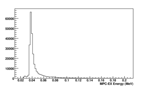
Figure 3.70: Energy distribution of MPC-EX tracks from single charged particles. The MIP peak at 36 MeV is clearly visible. In the analysis a cut is placed at $<$70 MeV to select charged particle tracks.

As we have no momentum measurement for charged tracks, all charged tracks are arbitrarily assigned an equal momentum of 1 GeV. The jet cluster algorithm is a seeded cone algorithm that uses every particle in the track list as seed for a cluster cone. The cluster cone is taken as a fixed radius in $\eta$ and $\phi$ space of 0.7 units. For each selection of a seed track, the cone algorithm and cluster axis are iterated until further iteration produces no change in the cluster axis. This cluster is recorded and the next seed is analyzed. Finally, from the list of all found clusters the cluster that contains the largest number of tracks is returned as a jet proxy for each MPC-EX arm.

Returning to our simple jet model consisting of four muons, in Figure 3.71 we show the resolution in $\eta$ and $\phi$ for charged track clusters with two, three and four charged particles for “jet” events with only charged tracks (the $\pi^{0}$ along the jet direction is not included in the simulation). The resolution improves slowly with the number of charged tracks used to determine the “jet” direction, as expected.

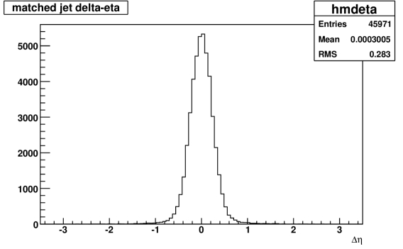
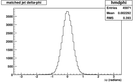
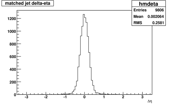
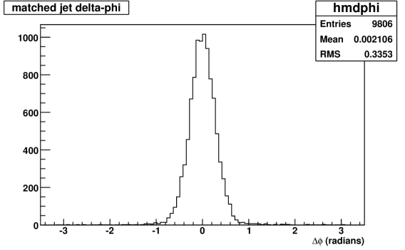
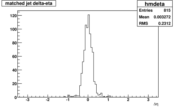
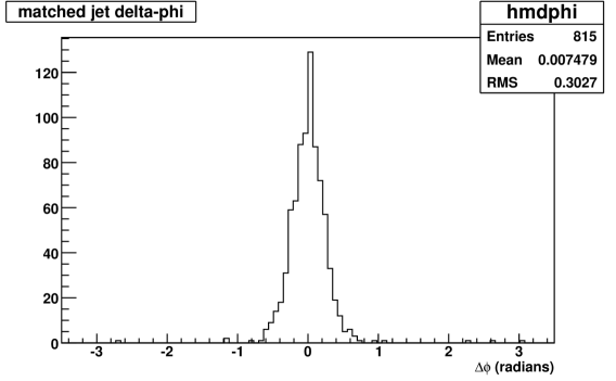
Figure 3.71: Resolution in $\eta$ and $\phi$ for a “jet” axis determined from charged particles reconstructed in the MPC-EX, for events with muons correlated with the “jet” axis without a $\pi^{0}$. The top row is for “jet” clusters determined with two or more charged particles, the middle with three or more, and the bottom with four or more charged tracks.

In Figure 3.72 we show the resolution in $\eta$ and $\phi$ for charged track clusters with two, three and four charged particles for “jet” events with charged tracks and a $\pi^{0}$ along the jet direction. The charged tracks found under these circumstances are clearly biased by the presence of the electomagnetic shower. In the case of only two tracks a clear splitting in the distribution of $\Delta\phi$ can be seen depending in whether both tracks are found on one side or another in $\phi$. The distribution in $\eta$ has also been affected, and is no longer purely Gaussian. Because the cone algorithm uses a fixed radius in $\eta$-$\phi$ space the actual distribution at forward rapidities on the face of the MPC-EX is a distorted ellipse, physically wider in the $\phi$ dimension. This is the reason that the splitting appears largest in $\Delta\phi$. The resolution improves slowly with the number of charged tracks used to determine the “jet” direction, and the splitting observed in phi is diminished. Nevertheless, the resolution at a fixed number of charged particles in these events is worse by about a factor of two.

Of course, this splitting effect is exaggerated in our toy model by placing the $\pi^{0}$ coincident with the jet axis. In real events there will be an event-by-event bias based on the number of charged tracks and their relative location with respect to any electromagnetic energy in the jet. If there is a spin dependence to this bias, the bias in the determination of the jet proxy axis will only exacerbate this effect.

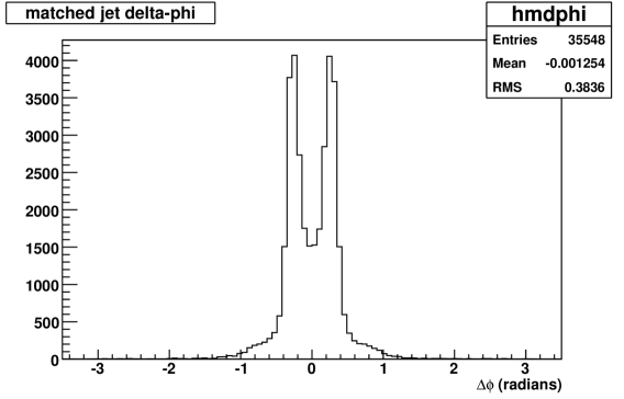
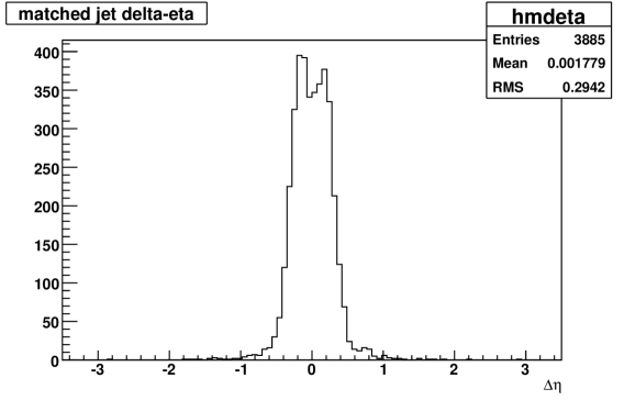
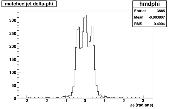
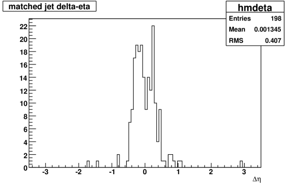
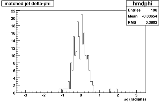
Figure 3.72: Resolution in $\eta$ and $\phi$ for a “jet” proxy determined from charged particles reconstructed in the MPC-EX, for events with muons correlated with the “jet” axis with a $\pi^{0}$ coincident with the jet axis. The top row is for “jet” clusters determined with two or more charged particles, the middle with three or more, and the bottom with four or more charged tracks.

3.6.2 Jet Axis Resolution in Pythia Events

In order to understand the resolution on the jet axis we can expect in real events, we simulated a set of Pythia $2\rightarrow 2$ hard scattering events in the MPC-EX detector. For these events the “true” jet axis was determined using the Fastjet [29] anti-$k_{T}$ jet-finding algorithm with a radius of 0.7 on the full Pythia event (no detector acceptance). The “true” jets found in this manner were required to have at leats 10 constituent particles and a $p_{T}>2$ GeV.

These events were then simulated in the full MPC-EX Monte Carlo, and the charged tracking and clustering algorithm described in Section 3.6.1 was applied. In the sections that follow we will be interested in correlating the jet proxy axis with a high momentum $\pi^{0}$ that is within $|\Delta\phi|<\frac{\pi}{2}$ in azimuthal angle of the jet proxy axis, so this requirement is also placed on the Pythia events. The jet proxy clusters were required to have at least two charged particles. (This is effectively a three particle requirement when the $\pi^{0}$ is included, but the $\pi^{0}$ is not used in the determination of the jet proxy direction.)

We then compare the jet proxy axis determined as described above with the “true” Pythia jet as determined by Fastjet. The jet proxy is associated with the closest “true” jet in $\Delta\eta$ - $\Delta\phi$ space, and the difference between the jet proxy and the “true” jet in $\Delta\eta$ and $\Delta\phi$ is determined. These distributions are shown in Figure 3.73.

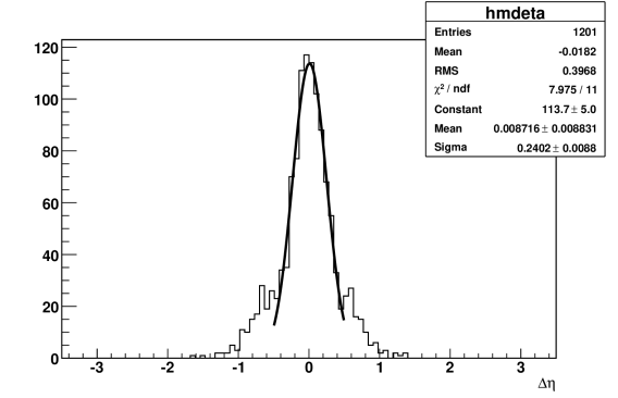
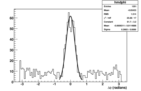
Figure 3.73: Resolution in $\eta$ (left) and $\phi$ (right) for a jet proxy determined from charged particles reconstructed in the MPC-EX for Pythia hard-scattering events. The resolution can be approximately described by a sigma of $\sim$0.3 units in both $\eta$ and $\phi$.

3.7 $\pi^{0}$ Correlations in Jets

In this section we describe simulations to estimate the sensitivity of the MPC-EX detector to an asymmetry of neutral pions around a fragmenting quark in transversely polarized $p$$+$$p$ collisions. Our strategy is as follows. First, we describe a Monte Carlo model that was developed to include the effects of finite transversity and Collins fragmentation in the final state distribution of hadrons from a fragmenting quark. Using this model we generate a sample of events with roughly the same single-particle asymmetry $A_{N}$ as that observed in neutral clusters in the PHENIX MPC, where the asymmetry is generated from the effects of transversity and Collins fragmentation. These events are put through a realistic simulation of the MPC-EX + MPC detectors, and are reconstructed and analyzed as physics data. The results of this exercise allows us to demonstrate the level of asymmetry due to transversity and Collins fragmentation that could be observed and make projections for a full event sample in real data.

3.7.1 The toyMC Monte Carlo Model

Simulations of the Collins asymmetry in jets in 200 GeV $p$$+$$p$ collisions requires a model that can produce a sample of particles from parton fragmentation with the asymmetry built-in to the kinematic distributions. At the start of the simulations for the MPC-EX no such model existed that implemented the best information available from SIDIS experiments in an event generator format. The toyMC model [59] was developed to address the need for just such an event generator.

The toyMC model starts with the event generator Pythia (version 6.421) [56], configured only to perform the initial partonic event. All fragmentation of the partons is disabled. In addition, because we seek a leading-order model consistent with the SIDIS extractions we will use to implement transversity and the Collins fragmentation functions, all QED and QCD radiation from the parton legs is disabled. Pythia is run with the standard QCD 2x2 hard scattering processes enabled (process ID’s 11,12,13,28,53,68 and 96) and we use TuneA Pythia parameter set, as this has been shown to better produce the pion cross sections (albiet at lower rapidities). The cross section for all sampled processes is 22.3mb. Configured in this manner the toyMC model allows us to benchmark the performance of the MPC-EX against current SIDIS analysis and data.

The spin of the incident protons are assigned randomly, and the spin of the scattered partons is set from the transversity distribution as parametrized in  [16] and  [17] at the scale of the hard interaction. Pions from quarks are generated according to the Collins fragmentations functions extracted from SIDIS and Belle data  [17] and parametrized based on the DSS fragmentation functions (FF’s), while pions from gluon fragmentation and all other particles are fragmented according to the spin-independent DSS FF’s. The choice of favored/unfavored Collins FF’s is made based on the fragmenting quark valence quark content of the hadron for charged pions, while it is assumed the the $\pi^{0}$ always fragments to pions according to the favored FF. The fragmentation functions are taken at the scale $\mu=p_{T}$ of the fragmenting parton. An example of the distribution of the Collins asymmetry as implemented in the toyMC model is shown in Figure 3.74.

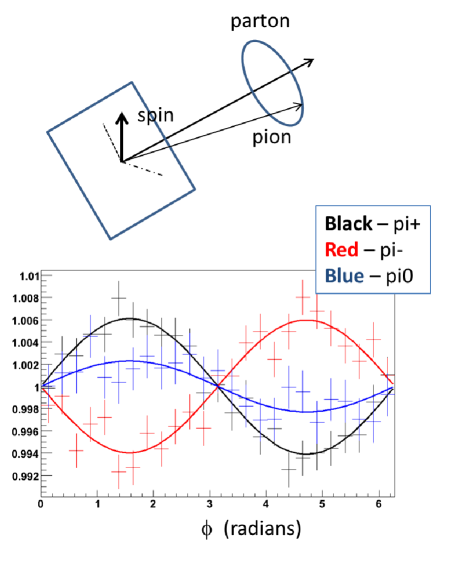
Figure 3.74: Sample toyMC distributions for pions, summed over all fragmenting quarks. The combination of transversity and the Collins FF’s yields an asymmetry patern where the $\pi^{+}$ and $\pi^{-}$ asymmetries are equal and opposite, and the $\pi^{0}$ asymmetry is the same sign as the $\pi^{+}$ asymmtery, although somewhat reduced. Note that the actual value of the asymmetries depends on the kinematic cuts and model parameters.

The toyMC model also implements the Sivers distributions as a set of event weights which can also be used to generate asymmetries for the final state particles. Because these are not relevant to the MPC-EX analysis they will not be discussed further here.

In order to benchmark the model and tune the asymmtries it generated for MPC-EX studies, we compare the single-particle $A_{N}$ for $\pi^{0}$ mesons in the MPC under various conditions in Figure 3.75. It should be noted that using the standard parametrizations for transversity and the Collins FF’s yields a vanishingly small asymmtery at large $x_{F}$ in 200 GeV $p$$+$$p$  collisions. This may in part be due to the fact that the transversity distribution above $x_{F}\sim 0.3$ is an extrapolation of the functional fit form and is not constrained by SIDIS data. Pushing transversity to the Soffer bound yields toyMC asymmetries that are similar to those observed in PHENIX (see Figure  3.76).

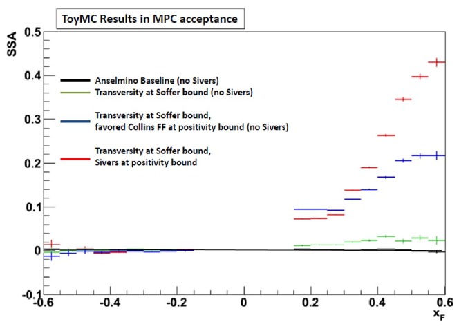
Figure 3.75: $A_{N}$ single spin asymmetries (single particle) for $\pi^{0}$ in the acceptance of the PHENIX MPC under various tunings of the toyMC model.

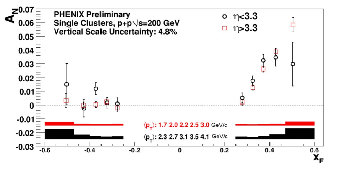
Figure 3.76: PHENIX preliminary results for the $A_{N}$ single spin asymmetries (single particle) for neutral clusters in the acceptance of the MPC.

3.7.2 Event Generation and Statistics

Two large samples of toyMC events were generated to simulate the extraction of the Collins asymmetry in the MPC-EX. The first sample of 4.9M events was generated with transversity set to the Soffer bound and the Collins FF’s set to the positivity limit. This set of events was used to examine the asymmetry for small systematic effects, such as an angular correlation between the extracted jet axis and the axis of the fragmenting parton. A second, larger set of 19.5M events was generated with transversity at the Soffer bound in order to match the single particle $A_{N}$ observed in PHENIX. This sample is the main sample used to test the sensitivity of the MPC-EX analysis to the Collins asymmetry. In both samples an event was written out from the Monte Carlo only if there was a $\pi^{0}$ and at least one charged particle in the acceptance of the MPC-EX. The small event sample corresponds to a sample luminosity of 0.10 $pb^{-1}$, while the large sample corresponds to 0.41 $pb^{-1}$.

In both cases the event vertex along the beamline was chosen according to a Gaussian distribution matched to the real distrbution of events in 200 GeV $p$$+$$p$ collisions. In the final analysis only events with a vertex between $\pm 70$ centimeters were used.

The output of the toyMC event generator was then put through the GEANT3-based PHENIX Integrated Simulation Application (PISA) in order to simulate the response of the MPC-EX, MPC and BBC detectors to the event, and the PHENIX reconstruction and analysis framework was used to turn the simulated hits into raw data quantities in a simulated DST. These DSTs were then analyzed to produce physics quantities.

3.7.3 $\pi^{0}$ Reconstruction

In jet events, reconstruction of $\pi^{0}$ mesons is done by single-track reconstruction for tracks with a total energy $>20$ GeV, and by two-track combinations for tracks with energies $<20$ GeV. The reconstruction method is described in section  3.1. Electromagnetic tracks are only required to have an associated MPC cluster and be flagged as the “closest” track in hough space. In addition, an electromagnetic track must not pass the charged particle cuts described above. This eliminates charged tracks that pass through the MPC-EX and shower in the MPC.

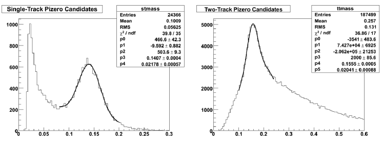
Figure 3.77: Invariant mass distributions for single-track (left) and two-track (right) $\pi^{0}$ reconstruction in toyMC jet events. The single-track $\pi^{0}$ distribution has less background, but lower statistics.

Figure  3.77 shows the resulting invariant mass distributions for single-track and two-track $\pi^{0}$’s in toyMC jet events. In general the single-track $\pi^{0}$ distribution has less background, particularly under the $\pi^{0}$ mass peak. Candidate $\pi^{0}$ mesons for correlations are selected by a $2.5\sigma$ mass cut in the reconstrcution, $0.105<m<0.205GeV$ for two-track $\pi^{0}$’s and $0.085<m<0.195GeV$ for the single-track reconstruction.

Because the two-track and single-track $\pi^{0}$’s are reconstructed in different energy ranges they sample different kinematics. In particular, the fragmentation $z=\frac{p_{\pi^{0}}}{p_{jet}}$ is higher for the single-track $\pi^{0}$’s, as shown in Figure 3.78. Because the Collins fragmentation function extracted from SIDIS measurements and used in toyMC is a strong function of the fragmentation $z$, the single-track pizero sample will have a larger asymmetry. Conversely, measuring the two-track and single-track pizero samples would allow some experimental sensitivity to the $z$ dependence of the Collins fragmentation function and would provide a greater constraint to theoretical models.

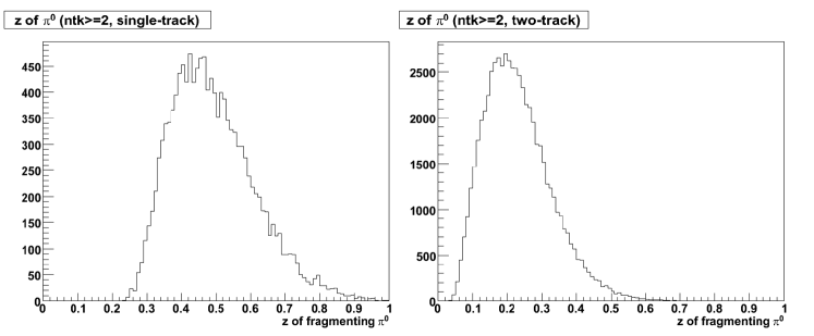
Figure 3.78: Distribution of fragmentation $z$ for single-track (left) and two-track (right) $\pi^{0}$ reconstruction. The sample of events chosen were events with two tracks found making up a charged cluster, with the $\pi^{0}$ on the same side as the cluster in azimuthal angle.

3.7.4 Jet Cluster Reconstruction

Jet cluster reconstruction proceeds by sorting MPC-EX tracks into charged track and electromagnetic track lists. For electromagntic tracks the total, calibrated energy deposited in the MPC-EX and MPC are used to define the track’s momentum. However, we have no momentum measurement for charged tracks, so all charged tracks are arbitrarily assigned an equal momentum of 1 GeV. The same jet cluster reconstruction is applied to both charged and EM tracks independently, but charged tracks and electromagnetic tracks are not combined in this analysis.

The jet cluster algorithm is a seeded cone algorithm that uses every particle in the track list as seed for a cluster cone. The cluster cone is take as a fixed radius in $\eta$ and $\phi$ space of 1.0 units for both electromagnetic and charged track clusters. For each selection of a seed track, the cone algorithm and cluster axis are iterated until further iteration produces no change in the cluster axis. This cluster is recorded and the next seed is analyzed. Finally, from the list of all found clusters the cluster that resulted in the highest transverse momentum is selected. It should be noted that in principle we could be less sensitive to backgrounds from gluon jets by reducing the cone radius, but this has not been explored in this analysis.

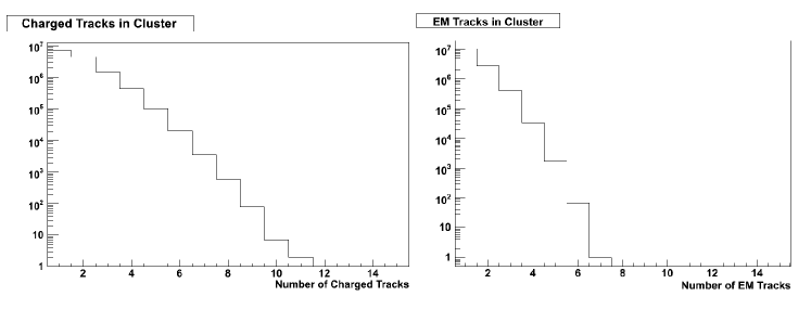
Figure 3.79: Distribution of number of tracks found in the highest $p_{T}$ cluster in a sample of toyMC jet events, for both charged jet clusters (left) and electromagnetic jet clusters (right).

In the analysis of jet cluster + $\pi^{0}$ correlations that follows, we require the jet cluster be comprised of two or more, or three or more particles, effectively making a three-particle or four-particle requirement for the jet when the $\pi^{0}$ requirement is added. For a complete dataset of real collisions the asymmetries obtained could be examined as a number of the particles required in the cluster in order to study systematic effects and improve signal-to-background, but that is not possible with the limited statistics available in this simulation.

3.7.5 Simulated Asymmetries

In this section we describe the simulated asymmetries based on the large statistics dataset, with single-particle $A_{N}$ asymmetries that are comparable to those observed in the MPC. The goal of this exercise is to benchmark the sensitivity of this analysis in terms of the minimum asymmetry that should be visible at a given integrated luminosity.

Charged Cluster - $\pi^{0}$ Correlations

The low asymmetry toyMC event sample is used to gauge the size of the asymmetry expected as well as the total available statistics given the simulated luminosity. Correlations are examined individually for both the single-track and two-track pizero samples. This statistical power in the Monte Carlo sample allows us to make meaningful correlations with charged particle jet clusters that have $>=2$ or $>=3$ charged partciles in the cluster. Charged cluster - $\pi^{0}$ correlations are obtained by selecting events with a charged cluster and a reconstructed $\pi^{0}$ within $\pm\pi/2$ in azimuthal angle. The Collins correlation angle $\phi$ is calculated and binned, and the result can be fit to extract the spin asymmetry.

As anticipated, the asymmetries are small in the two track sample. In fact, they are small enough that acceptance corrections at the level of 1% are required to be able to reliably extract the asymmetries (see Figure  3.80). This can be demonstrated by dividing the asymmetry distributions by a distribution generated by using the same events but with a random spin orientation, thus cancelling any spin-dependent effects and leaving only acceptance effects (see Figure  3.82). Figure  3.82 shows the result of this exercise, and a small Collins asymmetry is visible after the correction is made. We note that dividing the spin-dependent by the spin-randomized distributions in this way does artificially inflate the error bars on each point because the two samples are not independent. However, a small but sigificant spin-dependent asymmetry is still visible.

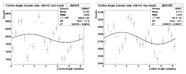
Figure 3.80: Collins angle asymmetries for two-track $\pi^{0}$’s correlated with charged clusters consisting of two or more particles in a charged cluster (left) and three or more particles (right). The shape of the distributions shows an acceptance effect that has not been accounted for.

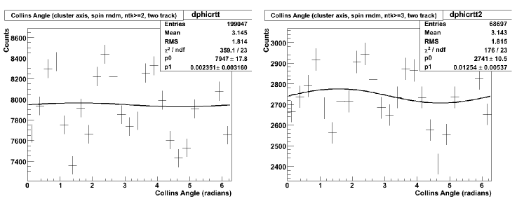
Figure 3.81: Collins angle asymmetries for two-track $\pi^{0}$’s correlated with charged clusters consisting of two or more particles in a charged cluster (left) and three or more particles (right). The spin asymmetry in these distributions is destroyed by randomizing the spins, leaving only acceptance effects.

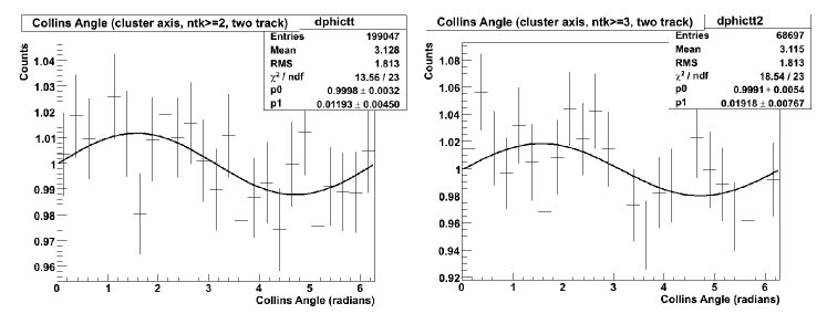
Figure 3.82: Correction of the acceptance effect in the two-track correlation sample after division by the spin-randomized distribution. Note that this process artificially inflates the error bars in the distribution because the two samples are correlated. A small Collins asymmtery is clearly visible after the correction. The correlation with charged track clusters containing two or more charged particles is shown on the left, and with three or more charged particles on the right.

Figure  3.83 shows the single-track $\pi^{0}$ asymmetries extracted from the large statistics toyMC sample for $\pi^{0}$’s correlated with different charged cluster samples. As with the two-track correlations, the spin-dependent distributions are divided by the spin-randomized distributions to eliminate acceptance effects. In the first sample two or more charged tracks are required to determine the charged cluster, while three or more are requred in the second sample. As expected, the extracted asymmetries are larger for the single-track correlations.

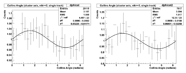
Figure 3.83: Collins angle asymmetries for single-track $\pi^{0}$’s correlated with charged clusters consisting of two or more particles in a charged cluster (left) and three or more particles (right).

The Monte Carlo samples allow us to estimate how many pairs will be obtained in a given sample of integrated luminosity as well as the magnitude of the anticipated asymmetry. The statistics in each bin in Collins correlation angle can be scaled to the total sampled luminosity of 49 $pb^{-1}$. These numbers then provide the basis for the statistical error in each bin. We assume a 60% beam polarization, and scale the anticipated asymmetry down by 0.6 to account for partial beam polarization. In addition, we also impose the trigger requirement that total energy in the MPC is greater than 35 GeV (see Section J). This requirement greatly reduces the statistical power of the two-track pizero sample by eliminating low-energy jets.

In Figure  3.84 we show the antipated asymmetry and statistical errors using single-track $\pi^{0}$’s correlated with a jet axis determined using three or more charged tracks. The anticipated statistical power is more than adequate to measure the expected asymmetries if the single particle $A_{N}$ is due to transversity and Collins fragmentation alone.

Figure 3.84: Anticipated statistics as a function of Collins angle for 49 $pb^{-1}$ sampled luminosity and average polarization of 60% using single-track $\pi^{0}$’s correlated with a jet axis determined by three or more charged particles. The blue curve is the anticipated asymmetry for the data sample from the Monte Carlo, corrected for the beam polarization of 60%.

The minumum asymmetry that can be observed is set by the ability to ascertain if more $\pi^{0}$’s go “left” with respect to the direction set by the spin axis and fragmenting parton, as opposed to “right”. To estimate the smallest asymmetry that could be observed we make maximum use of the statistical power of the data by dividing it into left and right, spin up and spin down samples, and calculating the asymmetry using the square root formula:

$$A_{N}^{raw}=\frac{\sqrt{N_{L}^{\uparrow}N_{R}^{\downarrow}}-\sqrt{N_{L}^{\downarrow}N_{R}^{\uparrow}}}{\sqrt{N_{L}^{\uparrow}N_{R}^{\downarrow}}+\sqrt{N_{L}^{\downarrow}N_{R}^{\uparrow}}}$$ (3.6)

Based on the assumed statistics and error propagation of the above formula, we can estimate the statistical error on the raw asymmetry $A_{N}^{raw}$ for each event selection. For Table  3.20 this analysis should be sensitive to a raw asymmetry down to one-seventh of the expected asymmetry, at the level of $3\sigma$. This means that this analysis will be capable of measuring a Collins asymmtery even if it is only responsible for as little as 27% of the overall single particle $\pi^{0}$ $A_{N}$ in the single-track correlations.

Table 3.20: Three-sigma statistical errors assuming 49 $pb^{-1}$ and 60% polarization for two events samples.

	Raw Asymmetry	3-$\sigma$ statistical
Event Selection	P = 0.6	error on $A_{N}^{raw}$
two-track $\pi^{0}$, $>=3$ tracks in charged cluster	0.011	0.014
single-track $\pi^{0}$, $>=3$ tracks in charged cluster	0.041	0.011

Electromagnetic Cluster - $\pi^{0}$ Correlations

As a demonstration, we also reconstruct clusters of electromagnetic tracks in this analysis. While electromagnetic clusters have the added benefit of yielding energy information, they are not appropriate for the determination of a Collins asymmetry through the correlation with $\pi^{0}$ mesons. The reason for this is simple - clusters determined with electromagnetic particles will contain the correlation that we are trying to measure, because most of the electromagnetic energy will come from $\pi^{0}$’s. This effect will become worse for higher momentum $\pi^{0}$’s because the cluster axis determination will be dominated by the $\pi^{0}$. In this case the correlation is increasingly like correlating the $\pi^{0}$ with itself. It is for this reason that the MPC alone cannot perform this type of analysis. Such an analysis has been attemped with the STAR FPD++  [39].

To demonstrate this effect, we show the correlations between $\pi^{0}$ mesons and an electromagnetic jet axis determined with three or more electromagnetic tracks in the MPC-EX in Figure  3.85. The asymmetries when correlating with an electromagnetic axis are essentially zero within errors.

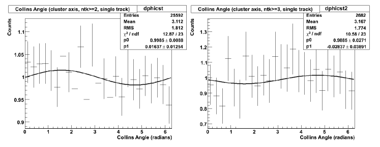
Figure 3.85: Collins angle asymmetries for single-track $\pi^{0}$’s correlated with electromagnetic clusters consisting of two or more electromagnetic tracks (left) and three or more electromagnetic tracks (right). The asymmtery is dramatically reduced compared to the charged cluster correlations, see Figure  3.83.

Jet Axis Resolution and Asymmetries

The resolution of the jet axis critically determines how the asymmetry measurement is diluted due to an imperfect knowledge of the fragmenting parton direction. Because the toyMC model is based on a simplified fragmentation scheme it is possible that this could yield a better resolution than one would anticipate from Pythia events. In Figure 3.86 we show the jet proxy axis resolution in $\eta$ and $\phi$ for toyMC events (averaged over spin orientation). The jet proxy axis resolution is similar to Pythia events, indicating that the simlified toyMC model has not resulted in an overly optimistic set of assumptions.

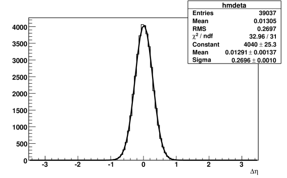
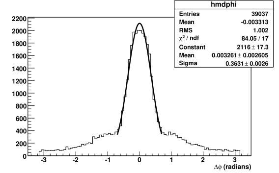
Figure 3.86: Resolution in $\eta$ (left) and $\phi$ (right) for a jet proxy determined from charged particles reconstructed in the MPC-EX for toyMC events. The jet proxy is required to have three or more charged particles. The resolution can be approximately described by a sigma of $\sim$0.3 units in both $\eta$ and $\phi$ and is consistent with the resolution obtained from Pythia events.

When charged particles (mostly $\pi^{+}$ and $\pi^{-}$) are used to reconstruct the jet direction it is possible that the asymmetries that these particles carry could bias the jet axis and either dilute or induce an asymmetry when correlated with $\pi^{0}$’s. However, any potential effect should be limited by the fact that the charged pions carry a roughly equal and opposite asymmetry, so that in the limit that a larger number of particles are used in the charged cluster any systematic effect should vanish.

This effect is too small to observe in the small asymmetry sample of events, but in Figure 3.87 we show the charged cluster asymmetry with respect to the jet axis for the large asymmetry sample of events. The large asymmetry sample enhances the effect, but it can be seen to diminish as a function of the number of charged particles required in the charged cluster. Studying the measured $\pi^{0}$ asymmetries as a function of the number of tracks in the charged cluster will provide a way to constrain any potential systematic error.

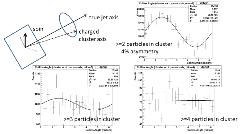
Figure 3.87: Asymmetry of the reconstructed charge cluster axis with respect to the parton axis for the large asymmetry sample of events. As a comparison the single particle $A_{N}$ is  20% in these events, substantially larger than the observed $A_{N}$, which magnifies the asymmetry of the charged cluster axis. This effect essentially disappears when three or more charged particles are required in the jet determination.

3.7.6 Effect of the Underlying Event

The previously described toyMC simulations included only the particles from jet fragmentation, and not additional particles from the underlying event (breakup of the target and projectile protons). In order to estimate this affect, a small sample of approximately 300k toyMC events were generated where the final jet particles were merged with an independent Pythia minimum bias event. These merged events were reconstructed following the same procedure as the jet events, and the resulting asymmetries compared.

Because of the lower statistics, a detailed comparison between the jet + minbias events and the low-asymmetry jet sample is not possible. However, we do note that even with the low statistics a significant asymmetry is still visible in the correlations. This gives us confidence that the presence of the underlying event does not destroy the correlations observed in the pure jet events.

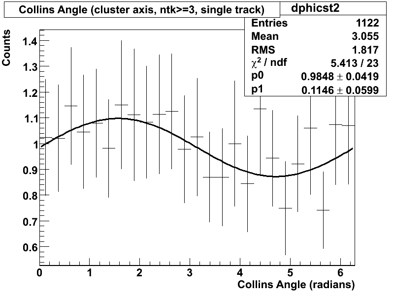
Figure 3.88: Angular correlations of $\pi^{0}$ mesons for clusters with three or more charged tracks in events where a toyMC jet event is merged with a Pythia minbias event. While the statistics are lower due to the smaller number of these events generated, a clear asymmetry is still visible.

Appendix J Event Rates

J.0.1 Event Rates

In this section we estimate the event rates for selected processes in p+p and d+Au collisions. All rates are for an MPC-EX in both the south and north arms in p+p, and in the deuteron going direction only in the case of d+Au collisions. In calculating event rates we start with latest guidance document from the RHIC Collider Accelerator Division (CAD) [37], which lists the store average luminosity for the various species and the delivered luminosity per week. We then assume a 60% up time for the PHENIX detector, a DAQ live time of 90%, and minbias trigger efficiencies (see Table J.1) for a 12 week run to obtain the luminosity sampled by PHENIX (see Table J.2). Note that we do not include an event vertex cut efficiency, as the MPC-EX analysis will be able to use essentially the full vertex distribution delivered by RHIC.

Table J.1: Efficiency factors used in the rate calculations. For A+A collisions the minimum bias trigger formed by the BBC is very close to 100% efficient, however in p+p and d+A collisions this is not the case.

Species	p+p 200 GeV	p+p 500 GeV	d+Au	Cu+Cu	Au+Au
min bias trigger eff	0.75	0.75	0.90	1.0	1.0

Table J.2: Luminosity guidance from CAD for RHIC. We then assume a 12 week run and a 60% uptime for PHENIX, a DAQ live time of 90% and a minbias trigger efficiency to obtain a PHENIX sampled integrated luminosity.

Species	p+p	p+p	d+Au	Cu+Cu	Au+Au
CM Energy	200 GeV	500 GeV	200 GeV	200 GeV	200 GeV
store average luminosity
($s^{-1}cm^{-2}$)	$3\times 10^{31}$	$1.2\times 10^{32}$	$1.8\times 10^{29}$	$5\times 10^{28}$	$3.5\times 10^{27}$
interaction rate (kHz)	1260	4200	328	124	17
lum/wk (pb-1wk-1)	10	40	0.060	0.016	0.0011
int. sampled lum (pb-1)	49	190	0.350	0.100	0.0071

NLO cross sections for $\pi^{0}$, direct and fragmentatation photons at 200 GeV were obtained from Werner Vogelsang, for p+p collisions at 200 GeV [60]. These cross sections were calculated using the CTEQ6M5 pdf’s, with the scale $\mu=p_{T}$, and no isolation cuts for the photons. The $\pi^{0}$ cross sections were calculated using the DSS fragmentation functions.These cross sections are plotted in Figure  J.1. As one approaches very high $p_{T}$ (near the luminosity limit) the direct photon production surpasses the pizero production due to the fact that the pizeroes arise from fragmentation.

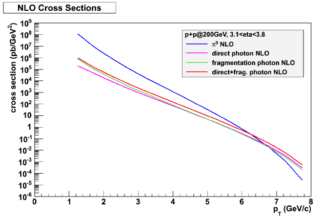
Figure J.1: NLO cross sections for pizero, direct photons, and fragmentation photons in the MPC-EX acceptance at 200 GeV as a function of transverse momentum.

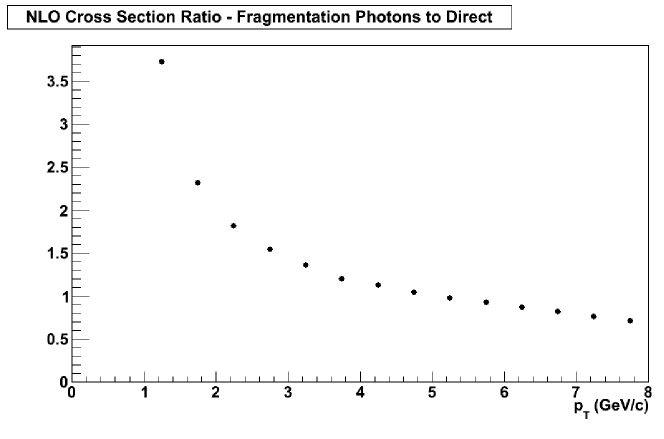
Figure J.2: Ratio of the NLO cross sections for fragmentation photons to direct photons in the MPC-EX acceptance at 200 GeV as a function of transverse momentum. From Werner Vogelsang.

In order to estimate the available statistics in a d+Au run we start with the NLO cross sections and assume $<N_{coll}>$ scaling so that the cross sections are scaled up by a factor of 8.3, the mean number of binary collisions in a minbias d+Au collsions as determined by a Glauber simulation  [2]. The estimated statistics in a RHIC d+Au run with 350 $nb^{-1}$ PHENIX integrated sampled luminosity (consistent with Table J.2) is shown in Table J.3 (without correction for suppression effects that will be present in d+Au collisions). The MPC-EX reconstruction efficiency is not included in these tables. These efficiencies are described for various cuts scenaries in Section 3.2.8.

Table J.3: Estimated statistics for dAu collisions, assuming PHENIX efficiencies (vertex and minbias trigger efficiency). MPC-EX reconstruction efficiencies are not included (see Section 3.2.8). These numbers are not adjusted for any suppression or shadowing effects.

$p_{T}$ (GeV/c)	$\pi^{0}$	photons (direct + frag.)	photon/$\pi^{0}$
1.0-1.5	$9.2\times 10^{8}$	$7.6\times 10^{6}$	0.0084
1.5-2.0	$8.2\times 10^{7}$	$1.5\times 10^{6}$	0.018
2.0-2.5	$1.1\times 10^{7}$	$3.5\times 10^{5}$	0.031
2.5-3.0	$1.8\times 10^{6}$	$9.0\times 10^{4}$	0.050
3.0-3.5	$3.3\times 10^{5}$	$2.5\times 10^{4}$	0.075
3.5-4.0	$6.5\times 10^{4}$	$7.2\times 10^{3}$	0.11
4.0-4.5	$1.3\times 10^{4}$	$2.0\times 10^{3}$	0.16
4.5-5.0	$2.5\times 10^{3}$	583	0.24
5.0-5.5	450	173	0.36
5.5-6.0	72	42	0.58
6.0-6.5	10	10	1.0

The estimated statistics in a transversely polarized RHIC p+p run with 49 $pb^{-1}$ PHENIX integrated sampled luminosity (consistent with Table J.2) is shown in Table J.4.

Table J.4: Estimated statistics for p+p collisions, assuming PHENIX efficiencies (vertex and minbias trigger efficiency). MPC-EX reconstruction efficiencies are not included (see Section 3.2.8).

$p_{T}$ (GeV/c)	$\pi^{0}$	photons (direct + frag.)
1.0-1.5	$3.2\times 10^{10}$	$2.7\times 10^{8}$
1.5-2.0	$2.8\times 10^{9}$	$5.0\times 10^{7}$
2.0-2.5	$3.7\times 10^{8}$	$1.2\times 10^{7}$
2.5-3.0	$6.0\times 10^{7}$	$3.0\times 10^{6}$
3.0-3.5	$1.1\times 10^{7}$	$8.3\times 10^{5}$
3.5-4.0	$2.2\times 10^{6}$	$2.3\times 10^{5}$
4.0-4.5	$4.3\times 10^{5}$	$7.0\times 10^{4}$
4.5-5.0	$8.5\times 10^{4}$	$2.0\times 10^{4}$
5.0-5.5	$1.5\times 10^{4}$	$5.2\times 10^{3}$
5.5-6.0	$2.3\times 10^{3}$	1433
6.0-6.5	317	333
6.5-7.0	32	63
7.0-7.5	2	10

Finally, we compare the NLO cross sections obtained from Werner Vogelsang with the output of Pythia (see Figure  J.3). The Pythia events were generated using the “Tune A” Pythia tune, which is matched to CDF and D0 data. In general, there are three sources of “direct” photons in Pythia: photons generated at the hard scattering vertex, fragmentation photons, and photons from QED radiation off the incoming quarks. We find that the cross section for photons from the hard scattering vertex in Pythia is a reasonable match to the NLO cross section, and fragmentation photons are approximately equal, also in agreement with the NLO calculations.

Figure J.3: NLO cross sections fom Werner Vogelsang compared the cross sections extracted from Pythia for $\pi^{0}$’s and direct photons. Direct photons from Pythia are selected only from processes that produce a photon at the hard scattering vertex, fragmentation photons and radiation from incoming quarks are shown as separate entries. The direct photon, fragmentation, and radiation cross sections are comparable in Pythia. from the hard scattering vertex.

J.0.2 Triggering

Because the MPC-EX preshower has no direct trigger capabilities we will rely on triggering in the MPC to select our event sample. At the antipated interaction rate of 328 kHz a rejection of about 330 is required to keep the DAQ bandwidth allocated to the MPC-EX physics at 1 kHz. As we are primarily interested in the deuteron-going direction for d+Au running we assume we will be triggering on only one MPC-EX. For polarized p+p collisions, we assume that the both north and south MPC’s will be utilized for triggering, but that the DAQ bandwidth allocated to MPC-EX physics is correspondingly higher at 2 kHz. At the antipiated interaction rate of 1.3 Mhz the required event rejection is 1300.

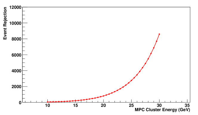
Figure J.4: Event rejection as a function of MPC cluster energy for the Pythia p+p 200 GeV event sample. For d+Au collisions the required rejection of approximately 330 is reached at a trigger cluster energy of 16.5 GeV. For p+p collisions the required event rejection of approximately 1300 is reached at a trigger energy of 22 GeV.

Figure J.4 shows the anticipated trigger rejection as a function of MPC cluster energy trigger threshold, based on the minbias Pythia event sample used for the direct photon analysis with full simulation through the PHENIX GEANT-based package PISA. Sufficient rejection is achieved in d+Au collisons at a trigger threshold of 16.5 GeV.

For jets in polarized p+p collsions we find that triggering on total energy in the MPC provides an improved trigger efficiency. Figure J.5 shows the anticipated trigger rejection as a function of total energy in the MPC, based on the minbias Pythia event sample used for the direct photon analysis with full simulation through the PHENIX GEANT-based package PISA. Sufficient rejection is achieved in p+p collisions at a total energy trigger threshold of 35 GeV.

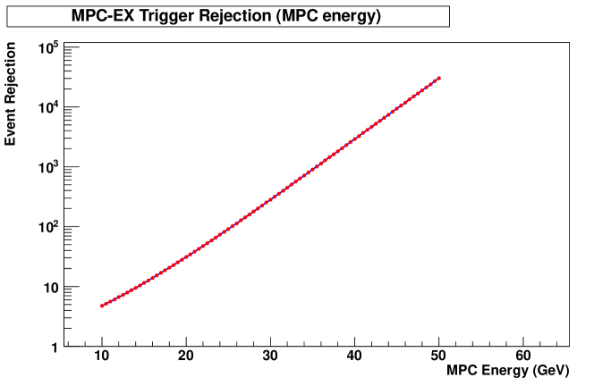
Figure J.5: Event rejection as a function of total MPC energy for the Pythia p+p 200 GeV event sample. For p+p collisons the required event rejection of approximately 1300 is reached at a trigger energy of 35 GeV.

Appendix K MPC-EX Collaboration

Brookhaven National Laboratory,

Upton, NY 11973, USA
E. Kistenev, A. Sukhanov

Chonbuk National University,

Jeonju, Korea
Eun-Joo Kim

Ewha Womens University,

Seoul, Korea
K.I. Hahn, D.H. Kim, S.Y. Han

Hanyang University,

Seoul, Korea
B.H. Kang, J.S. Kang, Y.K. Kim, J.S. Park

Iowa State University,

Ames, Iowa 50011, USA
S. Campbell, J.G. Lajoie, R. McKay, J. Perry, A. Timilsina

Los Alamos National Laboratory,

Los Alamos, New Mexico 87545, USA
J. Huang, X. Jiang, M. Leitch, M. Liu

University of California - Riverside,

Riverside, California 92521, USA
K.N. Barish, D. Black, L. Garcia, R.S. Hollis, A. Iordanova, R. Seto, W. Usher

Yonsei University, IPAP

Seoul, Korea
J.H Do, J.H. Kang, H.J. Kim, Y. Kwon, S.H. Lim, M. Song

Bibliography

- [1] A good description of the kolmogorov test can be seen at:. http://www.itl.nist.gov/div898/handbook/eda/section3/eda35g.htm.
- [2] Phenix analysis notes 633, 381 and 295.
- [3] Belle Collaboration, K. Abe et al. Measurement of azimuthal asymmetries in inclusive production of hadron pairs in e+ e- annihilation at Belle. Phys. Rev. Lett., 96:232002, 2006. arXiv:hep-ex/0507063, doi:10.1103/PhysRevLett.96.232002.
- [4] STAR Collaboration Collaboration, B. I. Abelev et al. Forward neutral-pion transverse single-spin asymmetries in collisions at . Phys. Rev. Lett., 101:222001, Nov 2008. Available from: http://link.aps.org/doi/10.1103/PhysRevLett.101.222001, doi:10.1103/PhysRevLett.101.222001.
- [5] STAR Collaboration, D.L. Adams et al. Analyzing power in inclusive and production at high with a 200 gev polarized proton beam. Phys. Lett. B, 265:462–466, 1991.
- [6] PHENIX Collaboration, A. Adare et al. Quantitative Constraints on the Opacity of Hot Partonic Matter from Semi-Inclusive Single High Transverse Momentum Pion Suppression in Au+Au collisions at sqrt() = 200 GeV. Phys. Rev., C77:064907, 2008. arXiv:0801.1665, doi:10.1103/PhysRevC.77.064907.
- [7] A. Adare et al. Cold Nuclear Matter Effects on J/psi Yields as a Function of Rapidity and Nuclear Geometry in Deuteron-Gold Collisions at sqrt() = 200 GeV. 2010. arXiv:1010.1246.
- [8] PHENIX Collaboration, A. Adare et al. High direct photon and triggered azimuthal jet correlations and measurement of for isolated direct photons in p+p collisions at gev. Phys. Rev. D, 82:072001, 2010. arXiv:hep-ph/1006.1347, doi:10.1103/PhysRevD.82.072001.
- [9] PHENIX Collaboration Collaboration, A. Adare et al. Suppression of back-to-back hadron pairs at forward rapidity in d+Au Collisions at = 200 GeV. 2011. * Temporary entry *. arXiv:1105.5112.
- [10] PHENIX Collaboration, S. S. Adler et al. Centrality dependence of direct photon production in s(NN)**(1/2) = 200-GeV Au + Au collisions. Phys. Rev. Lett., 94:232301, 2005. arXiv:nucl-ex/0503003, doi:10.1103/PhysRevLett.94.232301.
- [11] PHENIX Collaboration Collaboration, Stephen Scott Adler et al. Absence of suppression in particle production at large transverse momentum in S(NN)**(1/2) = 200-GeV d + Au collisions. Phys.Rev.Lett., 91:072303, 2003. arXiv:nucl-ex/0306021, doi:10.1103/PhysRevLett.91.072303.
- [12] The HERMES Collaboration Collaboration, A. Airapetian et al. Single-spin asymmetries in semi-inclusive deep-inelastic scattering on a transversely polarized hydrogen target. Phys. Rev. Lett., 94:012002, Jan 2005. Available from: http://link.aps.org/doi/10.1103/PhysRevLett.94.012002, doi:10.1103/PhysRevLett.94.012002.
- [13] A. Airapetian et al. Effects of transversity in deep-inelastic scattering by polarized protons. Physics Letters B, 693(1):11 – 16, 2010. Available from: http://www.sciencedirect.com/science/article/pii/S0370269310009457, doi:10.1016/j.physletb.2010.08.012.
- [14] M. Alekseev et al. Collins and sivers asymmetries for pions and kaons in muon–deuteron dis. Physics Letters B, 673(2):127 – 135, 2009. Available from: http://www.sciencedirect.com/science/article/pii/S0370269309000884, doi:10.1016/j.physletb.2009.01.060.
- [15] M.G. Alekseev et al. Measurement of the collins and sivers asymmetries on transversely polarised protons. Physics Letters B, 692(4):240 – 246, 2010. Available from: http://www.sciencedirect.com/science/article/pii/S0370269310009184, doi:10.1016/j.physletb.2010.08.001.
- [16] M. Anselmino, M. Boglione, U. D’Alesio, A. Kotzinian, F. Murgia, et al. Transversity and Collins functions from SIDIS and e+ e- data. Phys.Rev., D75:054032, 2007. arXiv:hep-ph/0701006, doi:10.1103/PhysRevD.75.054032.
- [17] M. Anselmino, M. Boglione, U. D’Alesio, A. Kotzinian, F. Murgia, et al. Update on transversity and Collins functions from SIDIS and e+ e- data. Nucl.Phys.Proc.Suppl., 191:98–107, 2009. arXiv:0812.4366, doi:10.1016/j.nuclphysbps.2009.03.117.
- [18] M. Anselmino, M. Boglione, U. D’Alesio, A. Kotzinian, F. Murgia, A. Prokudin, and S. Melis. Update on transversity and collins functions from sidis and data. Nuclear Physics B - Proceedings Supplements, 191(0):98 – 107, 2009. ¡ce:title¿Proceedings of the Ringberg Workshop¡/ce:title¿ ¡ce:subtitle¿New Trends in HERA Physics 2008¡/ce:subtitle¿. Available from: http://www.sciencedirect.com/science/article/pii/S0920563209003727, doi:10.1016/j.nuclphysbps.2009.03.117.
- [19] M. Anselmino et al. Extracting the Sivers function from polarized SIDIS data and making predictions. Phys. Rev., D72:094007, 2005. arXiv:hep-ph/0507181, doi:10.1103/PhysRevD.72.094007.
- [20] Nestor Armesto. Nuclear shadowing. J. Phys., G32:R367–R394, 2006. arXiv:hep-ph/0604108, doi:10.1088/0954-3899/32/11/R01.
- [21] BRAHMS Collaboration Collaboration, I. Arsene et al. Quark gluon plasma and color glass condensate at RHIC? The Perspective from the BRAHMS experiment. Nucl.Phys., A757:1–27, 2005. arXiv:nucl-ex/0410020, doi:10.1016/j.nuclphysa.2005.02.130.
- [22] BRAHMS Collaboration Collaboration, I. Arsene et al. Single-transverse-spin asymmetries of identified charged hadrons in polarized collisions at . Phys. Rev. Lett., 101:042001, Jul 2008. Available from: http://link.aps.org/doi/10.1103/PhysRevLett.101.042001, doi:10.1103/PhysRevLett.101.042001.
- [23] A. Bacchetta et al. Sivers single-spin asymmetry in photon-jet production. Phys. Rev. Lett., 99:212002, 2007.
- [24] Alessandro Bacchetta, Aurore Courtoy, and Marco Radici. First glances at the transversity parton distribution through dihadron fragmentation functions. Phys. Rev. Lett., 107:012001, Jun 2011. Available from: http://link.aps.org/doi/10.1103/PhysRevLett.107.012001, doi:10.1103/PhysRevLett.107.012001.
- [25] L.C. Bland. Transverse spin and rhic. arXiv:hep-ex/0602012.
- [26] F. Bradamante. Measurement of the collins asymmetries on transversely polarised protons. Transversity-2011 Workshop, 2011.
- [27] Stanley J. Brodsky, Dae Sung Hwang, and Ivan Schmidt. Final-state interactions and single-spin asymmetries in semi-inclusive deep inelastic scattering. Physics Letters B, 530(1-4):99 – 107, 2002. Available from: http://www.sciencedirect.com/science/article/pii/S0370269302013205, doi:10.1016/S0370-2693(02)01320-5.
- [28] Stanley J. Brodsky, Dae Sung Hwang, and Ivan Schmidt. Initial-state interactions and single-spin asymmetries in Drell-Yan processes. Nucl. Phys., B642:344–356, 2002. arXiv:hep-ph/0206259, doi:10.1016/S0550-3213(02)00617-X.
- [29] Matteo Cacciari, Gavin P. Salam, and Gregory Soyez. FastJet user manual. 2011. arXiv:1111.6097.
- [30] John C. Collins. Fragmentation of transversely polarized quarks probed in transverse momentum distributions. Nucl. Phys., B396:161–182, 1993. arXiv:hep-ph/9208213, doi:10.1016/0550-3213(93)90262-N.
- [31] John C. Collins. Leading-twist Single-transverse-spin asymmetries: Drell- Yan and Deep-Inelastic Scattering. Phys. Lett., B536:43–48, 2002. arXiv:hep-ph/0204004, doi:10.1016/S0370-2693(02)01819-1.
- [32] Umberto D’Alesio and Francesco Murgia. Parton intrinsic motion in inclusive particle production: unpolarized cross sections, single spin asymmetries, and the sivers effect. Phys. Rev. D, 70:074009, Oct 2004. Available from: http://link.aps.org/doi/10.1103/PhysRevD.70.074009, doi:10.1103/PhysRevD.70.074009.
- [33] Daniël and Boer. On a possible node in the sivers and qiu–sterman functions. Physics Letters B, 702(4):242 – 245, 2011. Available from: http://www.sciencedirect.com/science/article/pii/S0370269311007842, doi:10.1016/j.physletb.2011.07.006.
- [34] Fabio Dominguez, Cyrille Marquet, Bo-Wen Xiao, and Feng Yuan. Universality of Unintegrated Gluon Distributions at small x. Phys.Rev., D83:105005, 2011. arXiv:1101.0715, doi:10.1103/PhysRevD.83.105005.
- [35] K.J. Eskola, H. Paukkunen, and C.A. Salgado. EPS09: A New Generation of NLO and LO Nuclear Parton Distribution Functions. JHEP, 0904:065, 2009. arXiv:0902.4154, doi:10.1088/1126-6708/2009/04/065.
- [36] M.Adams et al. Design report of the central preshower detector for the d0 upgrade. 1996.
- [37] W. Fisher, T. Roser, M. Bai, J. Alessi, H. Huang, C. Montag, M. Blaskiewicz, and V. Schoefer. Rhic collider projections (fy2012-fy2016), 14 october 2011.
- [38] M. Chiu for the PHENIX Collaboration. Single Spin Transverse Asymmetries of Neutral Pions at Forward Rapidities at GeV. 2007. arXiv:0701031v1.
- [39] N. Poljak for the STAR Collaboration. Forward Jet-like Event Spin-dependent Properties in Polarized p+p Collisions at GeV. 2011. arXiv:1109.0360.
- [40] Leonard Gamberg and Zhong-Bo Kang. Single transverse spin asymmetry of prompt photon production. Phys.Lett., B718:181–188, 2012. arXiv:1208.1962, doi:10.1016/j.physletb.2012.10.002.
- [41] Francois Gelis, Edmond Iancu, Jamal Jalilian-Marian, and Raju Venugopalan. The Color Glass Condensate. Ann.Rev.Nucl.Part.Sci., 60:463–489, 2010. arXiv:1002.0333, doi:10.1146/annurev.nucl.010909.083629.
- [42] Heidelberg University Hans-Christian Schultz-Coulon. Electromagnetic calorimeters. 2005.
- [43] A. Hoecher, P. Speckmayer, J. Stelzer, J. Therhaag, E. von Toerne, and H. Voss. TMVA 4 Users Guide: Toolkit for Multivariate Data Analysis with ROOT, 2009. arXiv:physics/0703039.
- [44] Zhong-Bo Kang, Jian-Wei Qiu, Werner Vogelsang, and Feng Yuan. Observation concerning the process dependence of the sivers functions. Phys. Rev. D, 83:094001, May 2011. Available from: http://link.aps.org/doi/10.1103/PhysRevD.83.094001, doi:10.1103/PhysRevD.83.094001.
- [45] A. et. al. Karar. Investigation of avalanche photodiodes for em calorimeter at lhc. CMS Technical Note TN 95-135.
- [46] Dmitri Kharzeev, Eugene Levin, and Marzia Nardi. QCD saturation and deuteron nucleus collisions. Nucl.Phys., A730:448–459, 2004. arXiv:hep-ph/0212316, doi:10.1016/j.nuclphysa.2004.06.022,10.1016/j.nuclphysa.2004.06.022.
- [47] Dmitri Kharzeev and Marzia Nardi. Hadron production in nuclear collisions at RHIC and high density QCD. Phys.Lett., B507:121–128, 2001. arXiv:nucl-th/0012025, doi:10.1016/S0370-2693(01)00457-9.
- [48] Chris Kouvaris, Jian-Wei Qiu, Werner Vogelsang, and Feng Yuan. Single transverse-spin asymmetry in high transverse momentum pion production in collisions. Phys. Rev. D, 74:114013, Dec 2006. Available from: http://link.aps.org/doi/10.1103/PhysRevD.74.114013, doi:10.1103/PhysRevD.74.114013.
- [49] Larry D. McLerran and Raju Venugopalan. Computing quark and gluon distribution functions for very large nuclei. Phys. Rev., D49:2233–2241, 1994. arXiv:hep-ph/9309289, doi:10.1103/PhysRevD.49.2233.
- [50] Beau Meredith. A Study of Nuclear Effects Using Forward-Rapidity Hadron Production and Di-Hadron Angular Correlations in XXX d+A and p=P Collisions With the PHENIX Detector at RHIC. Ph.D. Thesis, University of Illinois and Urbana-Champaign, 2011.
- [51] PHENIX. PHENIX Analysis Notes AN633, AN381 and AN295. 2011.
- [52] Jefferson Lab Hall A Collaboration Collaboration, X. Qian et al. Single spin asymmetries in charged pion production from semi-inclusive deep inelastic scattering on a transversely polarized target at . Phys. Rev. Lett., 107:072003, Aug 2011. Available from: http://link.aps.org/doi/10.1103/PhysRevLett.107.072003, doi:10.1103/PhysRevLett.107.072003.
- [53] John P. Ralston and Davison E. Soper. Production of dimuons from high-energy polarized proton proton collisions. Nucl. Phys., B152:109, 1979.
- [54] Dennis W. Sivers. Single Spin Production Asymmetries from the Hard Scattering of Point-Like Constituents. Phys. Rev., D41:83, 1990. doi:10.1103/PhysRevD.41.83.
- [55] Torbjorn Sjostrand et al. High-energy-physics event generation with pythia 6.1. Comput. Phys. Commun., 135:238–259, 2001. arXiv:hep-ph/0010017.
- [56] Torbjorn Sjostrand, Stephen Mrenna, and Peter Z. Skands. PYTHIA 6.4 Physics and Manual. JHEP, 0605:026, 2006. arXiv:hep-ph/0603175, doi:10.1088/1126-6708/2006/05/026.
- [57] Mark Strikman and Werner Vogelsang. Multiple parton interactions and forward double pion production in pp and dA scattering. Phys.Rev., D83:034029, 2011. arXiv:1009.6123, doi:10.1103/PhysRevD.83.034029.
- [58] Berndt Surrow. Calorimetry in nuclear and particle physics experiments. 2006.
- [59] The toyMC Monte Carlo has been renamed ”tppmc” and is publicly available in Google Code. http://code.google.com/p/tppmc, 2011.
- [60] Werner Vogelsang. private communication, 2011.
- [61] Werner Vogelsang and Feng Yuan. Hadronic Dijet Imbalance and Transverse-Momentum Dependent Parton Distributions. Phys.Rev., D76:094013, 2007. arXiv:0708.4398, doi:10.1103/PhysRevD.76.094013.