Spectral Condition-Number Estimation of Large Sparse Matrices

Abstract

We describe a randomized Krylov-subspace method for estimating the spectral condition number of a real matrix $A$ or indicating that it is numerically rank deficient. The main difficulty in estimating the condition number is the estimation of the smallest singular value $\sigma_{\min}$ of $A$. Our method estimates this value by solving a consistent linear least-squares problem with a known solution using a specific Krylov-subspace method called LSQR. In this method, the forward error tends to concentrate in the direction of a right singular vector corresponding to $\sigma_{\min}$. Extensive experiments show that the method is able to estimate well the condition number of a wide array of matrices. It can sometimes estimate the condition number when running a dense SVD would be impractical due to the computational cost or the memory requirements. The method uses very little memory (it inherits this property from LSQR) and it works equally well on square and rectangular matrices.

1 Introduction

This paper discusses the problem of estimating the spectral condition number of a large and sparse matrix $A\in\mathbb{R}^{m\times n}$. Without loss of generality we assume that $m\geq n$ (we can estimate the condition number of $A^{T}$ if $n>m$). The main difficulty is in estimating the smallest singular value $\sigma_{\min}$ of $A$. Dense SVD algorithms can approximate $\sigma_{\min}$ well and their running time is predictable, but they are slow (their running time depends on the dimensions of the matrix, and not on the number of non-zeros entries in the matrix). More importantly, dense SVD algorithms require space that is proportional to $mn$ when the matrix is $m$-by-$n$, which is impractical for large sparse matrices. Likewise, if $A$ is square and a $LU$ factorization of $A$ can be computed then $\sigma_{\min}$ can be estimated efficiently from the factorization [12], however for some large sparse matrices space requirements due to fill-in make this method impractical.

Symmetrization is not always an effective way to address the problem. If we work with the Gram matrix $A^{T}A$, we cannot estimate condition numbers $\kappa(A)=\sigma_{\max}/\sigma_{\min}$ greater than $1/\sqrt{\epsilon_{\text{m}}}$, where $\epsilon_{\text{m}}$ is the unit roundoff (machine precision), unless the minimum singular value is well separated [21]. If we work with the augmented matrix

$$\begin{bmatrix}0&A^{T}\\ A&0\end{bmatrix}\;,$$

$\sigma_{\min}$ is transformed into a pair of eigenvalues $\pm\sigma_{\min}$ in the middle of the spectrum. Such eigenvalues are difficult to compute accurately with the Lanczos algorithm and its variants, and it is essentially impossible for such algorithms to determine whether there is an eigenvalue closer to zero than the one that has already been computed.

If one is interested in the smallest singular value of a large sparse matrix, then avoiding the impractical space requirements of dense SVD requires the use of a low-memory iterative method. Some Krylov-subspace methods estimate the condition number as the iteration progresses (e.g., LSQR). However, LSQR’s condition number estimator has some shortcomings that make it unreliable. We explain these in the next section.

The starting point of this paper is the following observation, which we explain in more detail in Section 3. Suppose $b$ is a vector in the column space of $A$, and let $Ax^{\star}=b$. Let $x^{(0)},x^{(1)},\dots$ be the iterates of a Krylov-subspace method applied to the problem $\arg\min\|Ax-b\|$ (all norms in this paper denote the $2$-norm unless stated otherwise). If we knew the forward error $d^{(k)}=x^{\star}-x^{(k)}$, we could use the Rayleigh quotients $\|Ad^{(k)}\|/\|d^{(k)}\|$ as an upper estimate on $\sigma_{\min}$. Now, if $b$ is also a random vector, then the iterates $x^{(k)}$ tend to generate at some point forward errors $d^{(k)}$ such that the Rayleigh quotient $\|Ad^{(k)}\|/\|d^{(k)}\|$ estimates $\sigma_{\min}$ well. The underlying reason is the tendency of Krylov-subspace methods to concentrate the forward error in the direction of a singular vector associated with $\sigma_{\min}$. This tendency is essentially the same as the tendency of the Lanczos algorithm to converge to outer eigenvalues first (see, e.g.,  [9, Section 7.3]). Both tendencies reflect the uneven convergence of Krylov subspaces to singular- or eigenspaces, one in the singular unsymmetric case (LSQR) and the other in the symmetric case (Lanczos or Conjugate Gradients). This is often seen as a flaw in LSQR and in Conjugate Gradients (LSQR is mathematically equivalent to Conjugate Gradients applied to $A^{T}Ax=A^{T}b$). These solvers converge slowly when the coefficient matrix $A$ is ill conditioned because it is difficult for them to get rid of the error in the right singular subspaces of $A$ that correspond to its smallest singular values. However, one can also exploit this flaw, which acts as a sieve that captures a vector from this subspace.

In this paper, we use this observation to design a Krylov-subspace method that can estimate $\sigma_{\min}$ (hence the spectral condition number $\mathbf{\sigma_{\max}/}\sigma_{\min}$) accurately. To have access to the forward error, our algorithm generates a random $x^{\star}$ and computes $b=Ax^{\star}.$ The algorithm then proceeds with using LSQR on the problem $\arg\min\|Ax-b\|$, meanwhile monitoring the value of $\|Ad^{(k)}\|/\|d^{(k)}\|$ and keeping the vector $d^{(\ell)}$ for which it is minimized. Very little memory is needed, as the algorithm’s memory usage is close to LSQR’s. As the iteration progresses, the estimate of $\sigma_{\min}$ does not deteriorate; we always keep the best $d^{(k)}$ found. However, it is undesirable to continue to run the algorithm when the estimate of $\sigma_{\min}$ is unlikely to improve. To that end, we design a set of stopping criteria that are tuned towards the algorithm’s goal of computing the condition number, as opposed to solving least-squares equations, which is what LSQR’s regular stopping criteria are tuned for. Some of our stopping criteria are the same as LSQR’s, but others are based on the algorithm’s knowledge of the forward error.

Our algorithm will never report an underestimate of $\sigma_{\min}$. Furthermore, in most cases it also produces a certificate vector that proves that the estimate of $\sigma_{\min}$ is indeed an upper bound. While we are unable to prove rigorous bounds on the quality of approximation, nor a bound on the number of iterations until convergence, extensive experiments indicate that our method does not incorrectly report significant overestimates of $\sigma_{\min}$, at least when $A$ is not close to being numerically rank deficient. When $A$ is close to numerical rank deficiency, the algorithm reports a condition number near $\epsilon_{\text{m}}^{-1}$, but the accuracy of the estimate is sometimes poor.

Our method also has some flaws. The main one is that it sometimes converges very slowly, making it essentially impossible to compute $\sigma_{\min}$. Our experience shows that the method always converges eventually, but that convergence might be too slow to be of practical use. There is no good way to determine how close the method is to termination, although it tends to behave consistently on related matrices (e.g., from the same application area). When $\kappa(A)$ is close to $\epsilon_{\text{m}}^{-1}$, the method sometimes overestimates $\sigma_{\min}$ by several orders of magnitude. The method sometimes converges very rapidly and sometimes very slowly. This is not related to the size of the problem and not to how ill conditioned it is, but to the distribution of singular values.

Even with these flaws, to the best of our knowledge this method is the only practical way to compute $\sigma_{\min}$ with reasonable accuracy (to within a factor of $2$ or better) on many large matrices. Our implementation of the method in MATLAB is freely available, and a C++ implementation is available inside the libSkylark library.

The rest of this paper is organized as follows. Section 2 surveys related work on condition number estimation. Section 3 presents a mathematical analysis of the quantity that we use to estimate $\sigma_{\min}$, to motivate the algorithm that we present in Section 4. Section 5 analyzes a unique stopping criteria that our method relies upon. Section 6 illustrates and explores the behavior of our algorithm using numerical experiments.

2 Related Work

The largest singular value $\sigma_{\max}$ of $A$ can be computed accurately using a bounded number of matrix-vector products involving $A$ and $A^{T}$. This can be done using the power method, for example, whose analysis for this application we explain in Section 4. The Lanczos method can reduce the number of matrix-vector products even further [25]. Random projection methods can also estimate $\sigma_{\max}$ [16].

Estimating $\sigma_{\min}$ is computationally more challenging, because applying the pseudoinverse is usually much harder than applying $A$ itself. In general, existing random projection methods cannot efficiently estimate $\sigma_{\min}$ unless a decomposition of $A$ is computed, or $A$ is low rank (or numerically low rank). If $A$ is low rank, random projection methods can be used to estimate the $k$th largest singular value, where $k$ is the (numerical) rank [16]. Another approach is to use iterative methods for computing singular triplets. Recently, variants of Lanczos that use implicit restarting, harmonic Ritz values and other advanced techniques to further accelerate the convergence to the smallest singular triplets have been proposed [24, 3]. Another approach for computing singular triplets (including the smallest singular triplets) is the JDSVD method [20] which extends the Jacobi-Davidson method for singular value problems. The PRIMME_SVDS [33] library implements an hybrid algorithm PHSVDS [32] which is based on carefully selecting an appropriate algorithm at each point of the computation.” Also worth mentioning is the inverse free preconditioned Krylov subspace method [14, 27].

The LINPACK condition-number estimator requires a triangular factorization of $A$ (see Higham’s monograph [18, Chapter 15] for details on this and related estimators). The Gotsman-Toledo [15] and the Bischof et al. [4] condition-number estimators, which are specialized to sparse matrices, also require a triangular factorization. Estimators that require a triangular factorization are less expensive than the SVD, but they still cannot be applied to huge matrices.

The LAPACK condition-number estimator estimates the 1-norm condition number [17] . Higham and Tisseur derive a block version of the LAPACK 1-norm condition number estimator [19]. Both methods are black-box in the sense that they require only matrix-vector products with the pseudoinverses of $A$ and $A^{T}$. One way to compute these products is using a factorization, but they can also be computed using an iterative solver. With an effective preconditioner, repeated applications of the pseudoinverse may be less expensive than the method that we propose, but without one our method is less expensive. Kenney et al. [22] describe a way to estimate the condition number of a square matrix using a single application of the inverse to one or several vectors. Vecharynski proposes a Rayleigh-quotient-type iteration that uses a single iteration of a preconditioned iterative solver to compute an approximate singular vector given an approximate singular value (which is estimated form the previous singular-vector estimate) [31]. Gaaf and Hochstenbach [12] propose to estimate the condition number of square matrices using the extended Krylov subspace. Computing a basis for the extended Krylov subspace requires applying the inverse of the matrix, so the method uses a $LU$ factorization of the matrix.

The spectral condition number measures the normwise sensitivity of matrix-vector products and linear systems to small perturbations in the inputs. There are methods that estimate more focused metrics, such as the sensitivity of individual components of the inputs or output [22]. Our method does not address this problem.

LSQR itself also estimates a condition number of $A$, the Frobenius condition number $\|A\|_{F}\|A^{+}\|_{F}$, where $A^{+}$ is the pseudoinverse of $A$. LSQR estimates the two norms by computing explicitly the Frobenius norm of two bidiagonal matrices that it computes as part of the algorithm, $B^{(t)}$ and $D^{(t)}$. The estimates rely on inequalities $\|B^{(t)}\|_{F}\leq\|A\|_{F}$ and $\|D^{(t)}\|_{F}\leq\|A^{+}\|_{F}$. However, this method has several serious shortcomings. First, the LSQR paper does not provide any evidence that the gap in the inequalities is small by the time the algorithm terminates. In particular, it appears difficult to come up with stopping criteria that will ensure that these estimates are accurate. Second, the inequalities depend on the theoretical (exact arithmetic) orthogonality of the Lanczos vectors, which are far from orthogonal when the algorithm is implemented in floating-point arithmetic.

As noted by Paige and Saunders [30], the spectral condition number can also be bounded using $\|B^{(t)}\|_{2}\|D^{(t)}\|_{2}$ but this is not done in practice (nor is it suggested by Paige and Saunders) since computing this quantity in each iteration is expensive.

Our method improves upon the condition number estimates of LSQR in several ways. First, we devise a way to approximate the spectral condition number cheaply in each iteration, so our algorithm estimates the spectral condition number instead of the Frobenius condition number, as is done by LSQR. The spectral condition number is more relevant for estimating the accuracy of linear solvers. Second, we use two estimators for $\sigma_{\min}$, one of which is similar in spirit to LSQR’s use of $\|D^{(t)}\|_{F}$ and the other completely novel, which only relies on properties that do hold in floating point. In particular, in addition to the novel estimator we use $R^{(t)}$ (another bidiagonal matrix formed by LSQR) instead of $D^{(t)}$ (as is done in LSQR), which is more robust to inexact arithmetic. Using $R^{(t)}$ is somewhat expensive, and this is why it is not used in LSQR, but because of the other estimator, our algorithm needs to use this estimator only once. Third, the other estimate that our algorithm computes comes with a vector that proves that our estimate is an upper bound on $\sigma_{\min}$ (the approximate singular vector). LSQR’s estimate also provides an upper bound, but it does not provide a certificate vector which materializes the bound. Fourth, the stopping criteria of our algorithm are designed specifically to discover that the estimate of $\sigma_{\min}$ is accurate; these criteria cannot be used in general in LSQR because they require knowledge of the forward error.

3 The Forward Error of Iterates on a Random Right-hand Side

In this section we introduce the idea that underlies our algorithm, namely that when applying LSQR to a random right-hand sides, the forward error in the iterates is rich in the direction of the smallest singular vector.

Let $x^{\star}$ be a random vector and let $b=Ax^{\star}$. Paige and Saunders explain in the LSQR paper [30, Section 7.1] that in exact arithmetic, the LSQR iterates are identical to the iterates of Conjugate Gradients [13, Section 11.3] when applied to the normal equations

$$A^{T}Ax^{\star}=A^{T}b\;.$$

Therefore, the $k$th iterate $x^{\left(k\right)}$ satisfies

$$x^{\left(k\right)}=\arg\min_{x\in\mathcal{K}_{k}(A^{T}A,A^{T}b)}\|x^{\star}-x\|_{A^{T}A}$$

where in the above $\mathcal{K}_{k}(A^{T}A,A^{T}b)$ is the $k$-dimensional Krylov subspace and $\left\|\;\cdot\;\right\|_{A^{T}A}$ denotes the norm $\left\|v\right\|_{A^{T}A}^{2}=v^{T}A^{T}Av$. We can therefore express $x^{(k)}$ as

$$x^{\left(k\right)} =p_{0}(A^{T}A)A^{T}b$$

for some degree-$(k-1)$ polynomial $p_{0}$ and the error as

$$x^{\star}-x^{\left(k\right)} =x^{\star}-p_{0}(A^{T}A)A^{T}b$$

$$=x^{\star}-p_{0}(A^{T}A)A^{T}Ax^{\star}$$

$$=p(A^{T}A)x^{\star}\;,$$

for a degree-$k$ polynomial $p(z)=1-zp_{0}(z)$.

Let us denote the thin SVD of $A$ and the eigendecomposition of its Gram matrix by

$$A = U\Sigma V^{T}$$

$$A^{T}A = V\Sigma^{2}V^{T}\;,$$

where $\Sigma^{2}=\text{diag}(\sigma_{1}^{2},\sigma_{2}^{2},\dotsc,\sigma_{n}^{2})$ for some $\sigma_{1}\geq\sigma_{2}\geq\cdots\geq\sigma_{n}=\sigma_{\min}\geq 0$. Then

$$\min_{x^{(k)}}\|x^{\star}-x^{\left(k\right)}\|_{A^{T}A}^{2} =\min_{p}\|p(A^{T}A)x^{\star}\|_{A^{T}A}^{2}$$

$$=\min_{p}\|p(V\Sigma^{2}V^{T})x^{\star}\|_{A^{T}A}^{2}$$

$$=\min_{p}\|Vp(\Sigma^{2})V^{T}x^{\star}\|_{A^{T}A}^{2}$$

$$=\min_{p}\sum_{i=1}^{n}\alpha_{i}^{2}\sigma_{i}^{2}p^{2}(\sigma_{i}^{2})\;,$$

where $\alpha_{i}=(V^{T}x^{\star})_{i}$ and the minimization is over all polynomials $p(z)$ of degree $k$ such that $p(0)=1$.

Now consider the $x^{(k)}$s, the forward errors $d^{(k)}=x^{\star}-x^{(k)}$, and the Rayleigh quotients

$$\frac{\|Ad^{(k)}\|}{\|d^{(k)}\|}\;.$$

In subsequent sections we experimentally show that these quantities tend to $\sigma_{\min}$ (and then diverge). To understand why this happens, let us express these quotients as

$$\frac{\|Ad^{(k)}\|^{2}}{\|d^{(k)}\|^{2}} = \frac{\|A(x^{\star}-x^{(k)})\|^{2}}{\|x^{\star}-x^{(k)}\|_{2}^{2}}$$

$$= \frac{\|AVp(\Sigma^{2})V^{T}x^{\star}\|^{2}}{\|Vp(\Sigma^{2})V^{T}x^{\star}\|^{2}}$$

$$= \frac{\|U\Sigma p(\Sigma^{2})V^{T}x^{\star}\|^{2}}{\|Vp(\Sigma^{2})V^{T}x^{\star}\|^{2}}$$

$$= \frac{\sum_{i=1}^{n}\alpha_{i}^{2}\sigma_{i}^{2}p^{2}(\sigma_{i}^{2})}{\sum_{j=1}^{n}\alpha_{j}^{2}p^{2}(\sigma_{j}^{2})}$$

$$= \sum_{i=1}^{n}\sigma_{i}^{2}\frac{\alpha_{i}^{2}p^{2}(\sigma_{i}^{2})}{\sum_{j=1}^{n}\alpha_{j}^{2}p^{2}(\sigma_{j}^{2})}\;.$$

LSQR chooses $p$ among all degree-$k$ polynomials with $p(0)=1$ so as to minimize the numerator $\sum_{i=1}^{n}\alpha_{i}^{2}\sigma_{i}^{2}p^{2}(\sigma_{i}^{2})$ in (3), which is equal to the square of the $A^{T}A$ norm of the forward error $d^{(k)}$. If $x^{\star}$ is a random vector with independent standard independent elements, then the $\alpha_{i}$s are also normal and independent, so we expect all the $\alpha_{i}$s to be roughly similar in magnitude; we do not expect very large or very small $\alpha_{i}$s. The term in the numerator involving $p^{2}(\sigma_{i}^{2})$ is multiplied by $\alpha_{i}^{2}\sigma_{i}^{2}$. If $\sigma_{n}<\sigma_{n-1}$, we expect the value of $p^{2}$ at $\sigma_{1}^{2},\ldots,\sigma_{n-1}^{2}$ to be small relative to $p^{2}(\sigma_{n}^{2})$, because the term involving $p^{2}(\sigma_{n}^{2})$ in the numerator of (3) is scaled by $\sigma_{n}^{2}$ ($\sigma_{n}=\sigma_{\min}$ is the smallest singular value), and the $\alpha_{i}$s are all similar in magnitude. In other words, to make the numerator of (3) small, the LSQR polynomial $p$ must assume small values at large $\sigma_{i}$s but can assume relatively large values at small $\sigma_{i}$s.

If $p^{2}$ indeed assumes a small value at $\sigma_{1}^{2},\ldots,\sigma_{n-1}^{2}$ but a relatively large value at $\sigma_{n}^{2}$ and if the $\alpha_{i}^{2}$s are all similar, then the expressions

$$\frac{\alpha_{i}^{2}p^{2}(\sigma_{i}^{2})}{\sum_{j=1}^{n}\alpha_{j}^{2}p^{2}(\sigma_{j}^{2})}$$

are much smaller than $1$ for $i=1,\ldots,n-1$ but close to $1$ for $i=n$ (these expressions sum to $1$). If this is the case, our Rayleigh quotient approximates $\sigma_{n}$. The analysis generalizes easily to multiple singular value at $\sigma_{\min}$.

We have not analyzed rigorously the quality of this approximation as a function of the spectral gap (between $\sigma_{\min}$ and the second smallest singular value) and of the random choice of $x^{\star}$. Neverthess, this mathematical analysis motivates our algorithm, which we describe in the next section.

4 The Algorithm

1:  Input: $A\in\mathbb{R}^{m\times n}$

2:  Parameters (defaults in parentheses): $c_{1}$ ($8\epsilon_{\text{m}}$), $c_{2}$ ($10^{-3}$), $c_{3}$ ($1/(64\cdot\epsilon_{\text{m}})$), $c_{4}$ ($\sqrt{\epsilon_{\text{m}}}$), $c_{1}^{\prime}$ ($4\epsilon_{\text{m}}$), and maxit.

3:  

4:  Estimate $\hat{\sigma}_{\max}=\sigma_{\max}$, along with a certificate $\hat{v}_{\max}$, using power iteration.

5:  $\hat{\sigma}_{\min}=\hat{\sigma}_{\max}$, $\hat{v}_{\min}=\hat{v}_{\max}$

6:  Draw a random vector $\hat{x}\in\mathbb{R}^{n}$ with independent normal entries

7:  $\tau\leftarrow\sqrt{2}\cdot\mathop{\operator@font erf}\nolimits^{-1}(c_{2})/\|\hat{x}\|$

8:  $x^{\star}\leftarrow\hat{x}/\|\hat{x}\|$

9:  $b\leftarrow Ax^{\star}$

10:  * $\beta^{(0)}\leftarrow\|b\|$, $u^{(0)}\leftarrow b/\beta^{(0)}$

11:  * $v^{(0)}\leftarrow Au^{(0)}$, $\alpha^{(0)}\leftarrow\|v^{(0)}\|$, $v^{(0)}\leftarrow v^{(0)}/\alpha^{(0)}$

12:  * $w^{(0)}\leftarrow v^{(0)}$

13:  * $x^{(0)}\leftarrow 0_{n\times 1}$

14:  * $\bar{\phi}^{(0)}\leftarrow\beta^{(0)}$, $\bar{\rho}^{(0)}\leftarrow\alpha$

15:  $T\leftarrow\text{maxit}$   {limit for $T$; usually reduced later}

16:  for $t=1,\dots,T$ do

17:     * $u^{(t)}\leftarrow Av^{(t-1)}-\alpha u^{(t-1)}$

18:     * $\beta^{(t)}\leftarrow\|u^{(t)}\|$

19:     * $u^{(t)}\leftarrow u^{(t)}/\beta^{(t)}$

20:     * $v^{(t)}\leftarrow A^{T}u^{(t)}-\beta^{(t)}v^{(t)}$

21:     * $\alpha^{(t)}\leftarrow\|v^{(t)}\|$

22:     * $v^{(t)}\leftarrow v^{(t)}/\alpha^{(t)}$

23:     * $\rho^{(t)}\leftarrow\left\|\left(\begin{array}[]{cc}\bar{\rho}^{(t-1)}&\beta^{(t)}\end{array}\right)\right\|$

24:     * $c^{(t)}\leftarrow\bar{\rho}^{(t-1)}/\rho^{(t)}$, $s^{(t)}\leftarrow\beta^{(t)}/\rho^{(t)}$

25:     * $\theta^{(t)}\leftarrow s^{(t)}\alpha^{(t)}$, $\bar{\rho}^{(t)}\leftarrow-c^{(t)}\alpha^{(t)}$

26:     * $\phi^{(t)}\leftarrow c^{(t)}\bar{\phi}^{(t-1)}$, $\bar{\phi}^{(t)}\leftarrow s\bar{\phi}^{(t-1)}$

27:     * $x^{(t)}\leftarrow x^{(t-1)}+(\phi^{(t)}/\rho^{(t)})w^{(t-1)}$

28:     * $w^{(t)}\leftarrow v^{(t)}-(\theta^{(t)}/\rho^{(t)})w^{(t-1)}$

29:     $R_{tt}^{(t)}\leftarrow\rho^{(t)}$   {Only diagonal and superdiagonal of $R$ are kept in memory}

30:     if $t>1$ set $R_{t-1,t}^{(t)}\leftarrow\theta^{(t-1)}$

31:     $d^{(t)}\leftarrow x^{\star}-x^{(t)}$

32:     if $d^{(t)}=0$ set $\hat{\sigma}_{\min}\leftarrow\hat{\sigma}_{\max}$, $\hat{v}_{\min}\leftarrow\hat{v}_{\max}$ and break for   {Due to finite precision arithmetic, when $\kappa\neq 1$ getting $d^{(t)}=0$ is extremely unlikely}.

33:     if $\|Ad^{(t)}\|\leq\hat{\sigma}_{\min}\|d^{(t)}\|$ then

34:        $\hat{\sigma}_{\min}\leftarrow\|Ad^{(t)}\|/\|d^{(t)}\|,$ $\hat{v}_{\min}\leftarrow d^{(t)}$

35:     end if

36:     if $\hat{\sigma}_{\min}/\hat{\sigma}_{\max}\leq c_{4}$ then $c_{1}\leftarrow c_{1}^{\prime}$

37:     if  $T=\text{maxit}$ and ($\frac{\|Ad^{(t)}\|}{\hat{\sigma}_{\max}\|x^{(t)}\|+\|b\|}\leq c_{1}$ or $\|d^{(t)}\|\leq\tau$ or $\hat{\sigma}_{\max}/\hat{\sigma}_{\min}\geq c_{3}$)  then

38:        $T\leftarrow\left\lceil 1.25t\right\rceil$

39:     end if

40:  end for

41:  Estimate $\tilde{\sigma}_{\min}=\sigma_{\min}(R^{(T)})$, using inverse power iteration

42:  $\tilde{\sigma}_{\min}\leftarrow\min(\tilde{\sigma}_{\min},\hat{\sigma}_{\min})$

43:  

44:  return  $\hat{\sigma}_{\max}/\hat{\sigma}_{\min}$, $\hat{\sigma}_{\max}$,$\hat{\sigma}_{\min}$, $\hat{v}_{\max}$ and $\hat{v}_{\min}$, $\tilde{\sigma}_{\min}$

Algorithm 1 The condition number estimation algorithm. Lines marked with * are inherited from LSQR. Some quantities, such as $\|\hat{x}\|$, $\|Ad^{(t)}\|$, $\|d^{(t)}\|$, and $\|b\|$, should be computed once and reused; the full expressions are shown multiple times for clarity.

This section describes our algorithm for estimating the condition number of $A$. A detailed pseudo-code description appears in Algorithm 1.

The algorithm starts by estimating $\sigma_{\max}$ and a corresponding certificate vector using power iteration on $A^{T}A$. By a certificate vector for an estimate $\hat{\sigma}_{\max}$ we mean a vector $v$ such that $\|Av\|/\|v\|=\hat{\sigma}_{\max}$ (and similarly for estimates of $\sigma_{\min}$). We perform enough iterations to estimate $\sigma_{\max}$ to within 10% of accuracy with probability at least $1-10^{-12}$. Using a bound due to Klein and Lu [23, Section 4.4], we find that given a relative error parameter $\epsilon$ and a failure probability parameter $\delta$, if we perform

$$\left\lceil\frac{1}{\epsilon}\left(\ln\left(2n\right)^{2}+\ln\left(\frac{1}{\epsilon\delta^{2}}\right)\right)\right\rceil$$

iterations, the relative error in our approximation is less than $\epsilon$ with probability at least $1-\delta$. For the parameters $\epsilon=10^{-1}$ and $\delta=10^{-12}$, 1004 iterations suffice even for matrices with up to $10^{9}$ columns. For $\epsilon=1/3$ and $\delta=10^{-12}$, only 298 iterations suffice for matrices with up to $10^{9}$ columns. (The accuracy of the $\sigma_{\max}$ estimate in the power method is typically much higher than predicted by this bound, but the additional accuracy depends on the gap between the largest and second-largest singular values; the bound that we use makes no assumption on the gap.) It is possible to use other methods to find $\hat{\sigma}_{\max}$ and $v$ (e.g. Lanczos). We chose power iteration because when we developed the algorithm existing theoretical results allow us to write an expression for the number of iterations as a function of $\epsilon$ and $\delta$, independent of the gap. Such strong bounds that guarantee high accuracy of $\sigma_{\max}$ are desirable since the stopping criteria we use for the estimation of $\sigma_{\min}$ depend on $\hat{\sigma}_{\max}$. Furthermore, for one singular pair, we empirically observed that the power method is typically faster than Lanczos and other iterative methods.

The main phase of the algorithm uses a modified LSQR iteration [29, 30, pages 50–51] designed to estimate $\sigma_{\min}$ and to produce a corresponding certificate vector. LSQR is a method for solving least squares problems $\min\|Ax-b\|_{2}$. At its core, LSQR uses the bidiagonlization procedure of Golub and Kahan to form iterates $u^{(0)},u^{(1)},\dots\in\mathbb{R}^{m}$, $v^{(0)},v^{(1)},\dots\in\mathbb{R}^{n},\alpha^{(0)},\alpha^{(1)},\dots\in\mathbb{R}$ and $\beta^{(0)},\beta^{(1)},\dots\in\mathbb{R}$ such that

$$U^{(t+1)}(\beta^{(1)}e_{1}) = b$$

$$AV^{(t)} = U^{(t+1)}B^{(t)}$$

$$A^{T}U^{(t+1)} = V^{(t)}(B^{(t)})^{T}+\alpha^{(t+1)}v^{(t+1)}e_{t+1}^{T}$$

where $U^{(t)}=\left[u^{(0)},u^{(1)},\cdots,u^{(t)}\right]$ and $V_{k}=\left[v^{(0)},v^{(1)},\cdots,v^{(t)}\right]$. LSQR uses these to find at iteration $t$ the optimal minimizer inside the Krylov subspace ${\cal K}_{t}(A^{T}A,A^{T}b)=span\{A^{T}b,(A^{T}A)A^{T}b,\dots,(A^{T}A)^{t-1}A^{T}b\}.$ In addition, LSQR forms additional bidiagonal matrices $R^{(0)},R^{(1)},\dots$ and estimates $\bar{\phi}^{(0)},\bar{\phi}^{(1)},\dots$ of the norm of the residual $r^{(t)}=b-Ax^{(t)}$. See [30] for details. We also remark that the Golub and Kahan bidiagonlization is closely related to the Lanczos tridiagonlization of the augmented matrix and of the Gram matrix, and that this connection is exploited by our algorithm.

The main idea in our algorithm is to use a random right-hand side so the forward error will tend to concentrate in the direction corresponding to $\sigma_{\min}$. To be able to access the forward error, we also generate the right-hand side in a way that gives us access to it. Specifically, our algorithm first generates a uniformly-distributed random vector $x^{\star}$ on the unit sphere by first generating a vector $\hat{x}$ with normally-distributed independent random components, and setting $x^{\star}=\hat{x}/\|\hat{x}\|$. The algorithm multiplies it by $A$ to produce a nearly consistent right-hand side $b$. While in exact arithmetic we would have had a consistent right hand side ($b=Ax^{\star}$), due to finite precision it is only nearly consistent: $\|b-Ax^{\star}\|\leq O(\epsilon_{\text{m}})\cdot\|A\|$.

Our algorithm modifies LSQR by adding a few steps to each iteration. At the end of each (standard) LSQR iteration, we have an updated approximate solution $x^{(t)}$ and an estimate of $\|r^{(t)}\|=\|Ax^{(t)}-b\|$, denoted by $\bar{\phi}^{(t)}$. The equality of $\bar{\phi}^{(t)}$ and $\|r^{(t)}\|$ depends on orthogonality of the Lanczos vectors, which lose orthogonality in floating point arithmetic as the algorithm progresses, so in practice $\bar{\phi}^{(t)}$ and $\|r^{(t)}\|$ may differ significantly. Our algorithm also computes the forward error $d^{(t)}=x^{\star}-x^{(t)}$ and $\|d^{(t)}\|$. We have

$$\left\|Ad^{(t)}\right\| = \left\|A\left(x^{\star}-x^{(t)}\right)\right\|$$

$$= \left\|b-Ax^{(t)}\right\|$$

$$= \left\|r^{(t)}\right\|\;,$$

which in exact arithmetic equals $\bar{\phi}^{(t)}$, but to improve the robustness of the algorithm we compute $\|Ad^{(t)}\|$ explicitly. (In our numerical experiments we have found $\bar{\phi}^{(t)}$ to be an accurate estimate, but we prefer to avoid any reliance on the orthogonality of the Lanczos vectors in our algorithm.) We also compute $\|x^{(t)}\|$.

Next, the algorithm computes the ratio $\|Ad^{(t)}\|/\|d^{(t)}\|,$ which like any Rayleigh quotient is an upper bound on $\sigma_{\min}$. If this ratio is the smallest we have seen so far, the algorithm treats it as an estimate of $\sigma_{\min}$ and stores both the ratio and the certificate $d^{(t)}$. When the algorithm terminates, it outputs the best ratio it has found and the corresponding certificate.

We use three stopping criteria. The first criterion, which is the one used by the standard LSQR algorithm for consistent systems, stops the algorithm when the normwise backward error [18, Section 7.1] drops below a threshold,

$$\frac{\left\|r^{(t)}\right\|}{\hat{\sigma}_{\max}\left\|x^{(t)}\right\|+\left\|b\right\|}\leq c_{1}\,,$$ (4.1)

where $\hat{\sigma}_{\max}$ is our estimate of $\|A\|$ and $c_{1}$ is a parameter that is set by default to $8\epsilon_{\text{m}}$. It has been observed experimentally [5] that for consistent systems, as long as $c_{1}$ is of the order of magnitude of $\epsilon_{\text{m}}$ or greater, this criterion will be eventually met in spite of the loss of orthogonality in the biorthogonalization process; however, the left-hand side of (4.1) does not seem to decrease much below the value required to satisfy the inequality [5].

In many cases our second stopping criterion will stop the algorithm well before the residual is that small. This second condition is

$$\left\|d^{(t)}\right\|\leq\frac{\sqrt{2}\cdot\mathop{\operator@font erf}\nolimits^{-1}(c_{2})}{\|\hat{x}\|}\;,$$ (4.2)

where $\mathop{\operator@font erf}\nolimits^{-1}$ is the inverse error function, computed using a numerical approximation, and $c_{2}$ is a parameter that is set by default to $10^{-3}$, which corresponds to $\mathop{\operator@font erf}\nolimits^{-1}(c_{2})\approx 8.9\times 10^{-4}$. This criterion is not used by LSQR; it requires knowledge of the error, which LSQR does not have in general. We explain this stopping criterion, and how the choice of $c_{2}$ affects the algorithm, in the next section.

The third stopping criterion is

$$\frac{\hat{\sigma}_{\max}}{\hat{\sigma}_{\min}}\geq c_{3}\,,$$ (4.3)

where $c_{3}$ is a parameter that is set by default to $1/(64\cdot\epsilon_{\text{m}})$. In other words, at this threshold we consider the matrix to be numerically rank deficient and we do not attempt to estimate the exact condition number. Standard LSQR uses a different condition number estimate in a similar stopping criterion, for regularization [30].

To achieve good accuracy even for matrices that are terribly ill conditioned (condition number close to $1/\epsilon_{\text{m}}$), the stopping criteria are refined in two additional ways:

1. If at some point we have

   $$\frac{\hat{\sigma}_{\max}}{\hat{\sigma}_{\min}}\geq c_{4}\,,$$

   where $c_{4}$ is a parameter that is set by default to $\sqrt{\epsilon_{\text{m}}}$, we set $c_{1}$ (residual-based stopping threshold) to $c_{1}^{\prime}$, which is set by default to $4\epsilon_{\text{m}}$. The rationale is that when the matrix is ill conditioned, the residual based test is less accurate so we lower threshold to compensate.

2. Even when the method detects convergence using one of its three criteria (small residual, small error, and numerical rank deficiency), it keeps iterating. The number of extra iterations is one quarter of the number performed until convergence was detected. This rule is a heuristic that tries to improve the accuracy of the condition number estimate. The cost of this heuristic is obviously limited and it can be turned off by the user.

In addition, our algorithm also stores the matrix $R^{(t)}$, one of two bidiagonal matrices that LSQR incrementally constructs but normally discards. In exact arithmetic, the singular values of $R^{(t)}$ converge to the singular values of $A$ [7, 10]. Once the algorithm terminates, we compute $\tilde{\sigma}_{\min}\approx\sigma_{\min}(R^{(t)})$; if it is smaller than the best $\|Ad^{(t)}\|/\|d^{(t)}\|$ estimate, we output both estimates. One estimate ($\tilde{\sigma}_{\min}$) is tighter, but it comes with no certificate vector; the other is looser, but comes with a certificate. Generating the certificate for the Lanczos estimate requires storing the Lanczos vectors or repeating the iterations. The former is obviously too expensive, while the latter might be redundant if the user is satisfied with the certificate already computed. We note that the singular values of $R^{(t)}$ tend to converge first to large singular values of $A$, so this estimate is not very likely to be better than $\|Ad^{(t)}\|/\|d^{(t)}\|$.

Storing $R^{(t)}$ and estimating $\sigma_{\min}(R^{(t)})$ is relatively inexpensive since $R^{(t)}$ is bidiagonal. We estimate it by running inverse iteration on $R^{(t)}$, again performing enough iterations to get to within 10% of accuracy with very high probability ($1-10^{-12}$; this is a parameter in the code). The cost of a single inverse power iteration is only $O(t)$. Since we use power-iteration, the error in $\tilde{\sigma}_{\min}$ is one sided: it is always the case that $\tilde{\sigma}_{\min}\geq\sigma_{\min}(R^{(t)})$ (because it is generated by a Rayleigh quotient). Also, $\sigma_{\min}(R^{(t)})\geq\sigma_{\min}$. Therefore, $\tilde{\sigma}_{\min}$ is also an upper bound on $\sigma_{\min}$, not just an estimate. We remark that $\tilde{\sigma}_{\min}$ is guaranteed to be an upper bound on $\sigma_{\min}$ only in exact arithmetic. In floating point, it is possible for $\tilde{\sigma}_{\min}$ to drop below $\sigma_{\min}$.

5 Analysis of the Small-Error Stopping Criterion

We now explain the second stopping criteria (4.2). Suppose that the smallest singular value of $A$ is simple and that it is well separated from the next smallest singular values. Let $x^{\star}=\sum_{i=1}^{n}\alpha_{i}v_{i}$ be the initial vector represented in the basis of the right singular vectors of $A$. As LSQR progresses towards finding $x^{\star}$ it will tend initially to resolve components in the direction of the largest singular vectors. Since the $v_{n}$ direction is not present in $x^{(0)}=0$ we expect it to be not present during the initial iterations, i.e., $(v_{n})^{T}x^{(t)}\approx 0$. This implies that we expect for the initial iterations to have $|(v_{n})^{T}(x^{\star}-x^{(t)})|\approx|\alpha_{n}|$ so $\|x^{\star}-x^{(t)}\|\geq\alpha_{n}$. Now, at some point in the iteration, the solution $x^{(t)}$ will be roughly $x^{(t)}\approx\sum_{i=1}^{n-1}\alpha_{i}v_{i}$, i.e., the error remains mostly in the direction of the smallest singular subspace, but the $v_{n}$ direction is not present at all. At that point, $\|x^{\star}-x^{(t)}\|\approx|\alpha_{n}|$. LSQR will now start to resolve that error at least partially and the norm of the error will decrease below $|\alpha_{n}|$. If we stop the iteration when $\|x^{\star}-x^{(t)}\|\gg|\alpha_{n}|$, the error is unlikely to be a good estimate of a small singular vector. If we stop when $\|x^{\star}-x^{(t)}\|\leq|\alpha_{n}|$ we will likely have a good estimate of a small singular value. Ideally, we want to stop immediately when $\|x^{\star}-x^{(t)}\|$ drops below $|\alpha_{n}|$. Stopping later (when the error is much smaller than $|\alpha_{n}|$) does not do any harm, since we report the best Rayleigh quotient seen, but it does not improve the estimate by much.

The second stopping criteria is designed so that the test passes only if the condition $\|x^{\star}-x^{(t)}\|\leq|\alpha_{n}|$ holds with high probability. It is based on the following proposition.

Proposition 1.

Suppose that $x^{\star}=\hat{x}/\|\hat{x}\|$ where $\hat{x}$ is a vector with normally-distributed independent random components, and assume $x^{\star}=\sum_{i=1}^{n}\alpha_{i}v_{i}$ be $x^{\star}$ represented in the basis of the right singular vectors of $A$. If

$$\|x^{\star}-y\|\leq\frac{\sqrt{2}\cdot\mathop{\operator@font erf}\nolimits^{-1}(\delta)}{\|\hat{x}\|}$$

then $\|x^{\star}-y\|\leq|\alpha_{n}|$ holds with probability of at least $1-\delta$ for $0<\delta<1$.

Proof.

Let $\hat{y}=\|\hat{x}\|y$ and $\hat{\alpha}_{n}=\|\hat{x}\|\alpha_{n}$. Obviously, $\|x^{\star}-y\|\leq|\alpha_{n}|$ if and only if $\|\hat{x}-\hat{y}\|\leq|\hat{\alpha}_{n}|$. Therefore, if we find a value $\tau$ such that $\Pr(|\hat{\alpha}_{n}|\geq\tau)\geq 1-\delta$ then the condition $\|\hat{x}-\hat{y}\|\leq\tau$ implies that $\|\hat{x}-\hat{y}\|\leq|\hat{\alpha}_{n}|$, and hence $\|x^{\star}-y\|\leq|\alpha_{n}|$, with a probability of at least $1-\delta$. Since $\|v_{n}\|=1$ we have $\hat{\alpha}_{n}\sim N(0,1)$. Therefore,

$$\Pr(|\hat{\alpha}_{n}|\geq\sqrt{2}\cdot\mathop{\operator@font erf}\nolimits^{-1}(\delta))=1-\delta\,,$$

so $\tau=\sqrt{2}\cdot\mathop{\operator@font erf}\nolimits^{-1}(\delta)$ can be used. The condition $\|\hat{x}-\hat{y}\|\leq\tau$ is now equivalent to $\|x^{\star}-y\|\leq\tau/\|\hat{x}\|$ which is exactly the criteria in the proposition statement. ∎

The choice of $c_{2}$ in the algorithm determines our confidence that $\|x^{\star}-x^{(t)}\|$ dropped below $|\alpha_{n}|$. We use a default value of $10^{-3}$, which implies a small probability of failure, but not a tiny one. The user can, of course, change the value if he or she needs higher confidence (in either case the error is one sided). Another approach is to use a much larger $c_{2}$ and to repeat the algorithm $\ell$ times (possibly in a single run, exploiting matrix-matrix multiplies), say $\ell=3$. The probability that we succeed in at least one run is at least $1-c_{2}^{\ell}$. For $c_{2}=10^{-2}$, say, setting $\ell=3$ or so should suffice. In our experience it is better to make $c_{2}$ smaller than to set $\ell>1$, but we did not do a formal analysis of this issue.

If the smallest singular value is multiple (associated with a singular subspace of dimension $k>1$), our situation is even better, because we can stop when $x^{\star}-x\approx\sum_{i=n-k+1}^{n}\alpha_{i}v_{i}$, when $\|x^{\star}-x\|\approx\sqrt{\alpha_{n-k+1}^{2}+\cdots+\alpha_{n}^{2}}$, which is even more likely to be larger than our stopping criterion.

When the smallest singular value is not well separated, the stopping criterion is still sound but the Rayleigh quotient estimate we obtain is not as accurate, because in such cases $x^{\star}-x$ tends to be a linear combination of singular vectors corresponding to several singular values. These singular values are all small, but they are not exactly the same, thereby pulling the Rayleigh quotient up a bit.

6 Numerical Investigations

This section illustrate and explore the behavior of our algorithm using numerical experiments.

6.1 Experiments on Synthetic Matrices

We begin by exploring the behavior of our method on synthetic $1000$-by-$400$ full-rank real matrices with prescribed singular values and random singular vectors.

The first matrix has 10 singular values at $10^{-8}$, 300 that are distributed logarithmically between $10^{-3}$ and $10^{-2}$, and 90 at $1$. The large gap between the smallest singular value and the next larger one makes the problem relatively easy for our algorithm.

Figure 6.1: The behavior of the method on one matrix described in the text. The vertical lines indicate the iterations at which the stopping criterion was triggered (green), and the iteration at which the algorithm would have returned (after performing 25% extra iterations; we ran the algorithm longer in this case).

Figure 6.1 shows the behavior of our method on one matrix generated with this spectrum. In the first 90 iterations or so the backward error (left-hand side in (4.1)) diminishes logarithmically; the norm of $x^{(t)}-x^{\star}$ drops a bit but then stops dropping much. These two effects cause our estimate $\hat{\sigma}_{\min}$ to also diminish roughly logarithmically. The Lanczos estimate $\sigma_{\min}(R^{(t)})$ drops a bit initially but stagnates from iteration 30 or so. What is happening up to iteration 90 or so is that Golub-Kahan bidiagonalization resolves the singular values in the $10^{-3}$-to-$10^{-2}$ cluster, while LSQR removes much of the projection of the corresponding singular vectors from the residual and from the error. Around iteration 160 Lanczos has resolved enough of the spectrum in the $10^{-3}$-to-$10^{-2}$ cluster and the smallest singular value of $R^{(t)}$ starts moving toward $10^{-8}$. At that point, most of the remaining error consists of singular vectors corresponding to the singular value $10^{-8}$, which causes our estimate to be accurate (to within 9 decimal digits!). The norm of $x^{(t)}-x^{\star}$ is still large, because the error contains a significant component in the subspace associated with the $10^{-8}$ singular values. At this point, around iteration 225, when the topmost black curve starts dropping again, LSQR starts to resolve the error in this subspace, the backward error starts decreasing again, the norm of $x^{(t)}-x^{\star}$ starts decreasing, which causes stopping criterion (4.2) to be met about 30 iterations later.

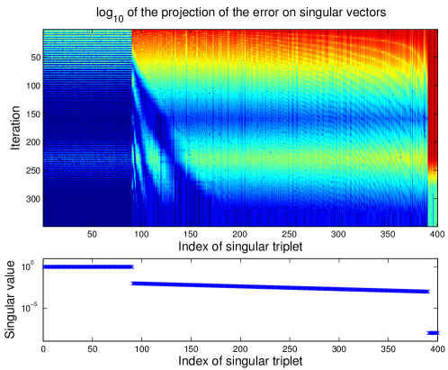
Figure 6.2: The projection of the forward error on the right singular vectors in the experiment shown in Figure 6.1. The bottom plot shows the singular values of $A$ and the top image shows the projections. Blue represents values near $\epsilon_{\text{m}}$; green represents values near $\sqrt{\epsilon_{\text{m}}}$; and red represents values near $1$.

Figure 6.2 visualizes the behavior described in the previous paragraph by plotting the projection of the forward error on the right singular vectors. We see that up to around iteration 50, the error associated with singular spaces associated with singular values other than $1$ remains very large. From that point on to about iteration 150, the error in subspaces corresponding to values between $10^{-3}$ and $10^{-2}$ is resolved, but the error associated with the singular value $10^{-8}$ is still very large. This is a point where our method finds the smallest singular value and its certificate (the error). As LSQR starts to resolve the error in the $10^{-8}$ singular subspace, the errors in the $10^{-3}$ to $10^{-2}$ subspaces grows (perhaps due to loss of orthogonality) but they are reduced again later.

The method yielded similar results when the smallest singular value was moved down to $10^{-13}$, with convergence after about 440 iterations and an estimate that is correct to within 5 decimal digits. The value $\sigma_{\min}=10^{-13}$ is about the lower limit for which the $\|d^{(t)}\|$ stopping criterion is useful.

When $A$ is rank deficient there are infinitely many solutions to the system $Ax=b$. The solution $x^{\star}$, which was generated randomly, has no special property that distinguishes it from other solutions (like minimum norm), so no least-squares solver can recover $x^{\star}$. Therefore, it is unlikely $\|d^{(t)}\|$ will become small enough to cause our method to stop. In this case, the method stops because the residual eventually becomes very small (close to $\epsilon_{\text{m}}$) or because the estimated condition number becomes too big (stopping condition (4.3)). In Figure 6.3 we illustrate the behavior of the algorithm on a rank deficient matrix; the matrix has 10 singular values that are $10^{-16}$ (numerical zeros), 300 distributed logarithmically between $10^{-3}$ and $10^{-2}$, and 90 at $1$.

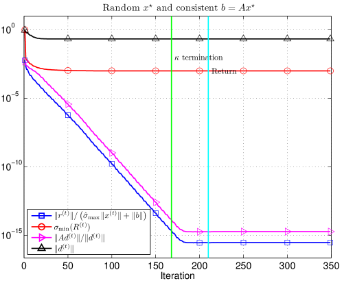
Figure 6.3: The behavior of the method on a numerically rank deficient matrix described in the text. Termination here occurred due to criterion (4.3).

The algorithm stopped because the condition number got too big; however a few iterations later it would have stopped because $\|r^{(t)}\|$ became too small (stopping condition (4.1)). Our estimate is not accurate (around $1.8\times 10^{-15}$, a relative error of $18$), but it still indicates to the user that the matrix is numerically rank deficient. Stopping criteria (4.1) and (4.3), and the relatively-inaccurate estimates they yield, are triggered only when the matrix is close to rank deficiency (condition number of about $10^{14}$ or larger).

Can

$$\|\arg\min_{x}\|Ax-b\|_{2}\|_{2}^{-1}$$

estimate $\sigma_{\min}$ if we take $b$ to be random unit vector? If $A$ has fewer columns than rows or is rank deficient, then with high probability a random $b$ is not in the column space of $A$. On some matrices, the minimizer has a norm that is larger than the norm of $b$ by about a factor of $\sigma_{\min}^{-1}$. However, unless there is a large gap between the smallest singular values and the rest, the minimizer has a smaller norm and the norms ratio fails to accurately estimate $\sigma_{\min}^{-1}$.

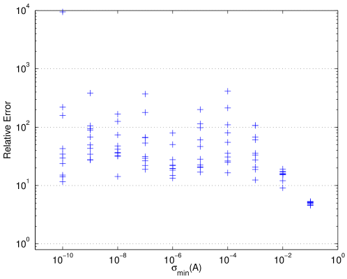
Figure 6.4: Estimating $\sigma_{\min}$ by $\|A^{+}b\|^{-1}$ for a unit-length random $b$ with normal independent components.

Figure 6.4 shows the relative errors in this estimate for matrices whose singular values are distributed linearly between $\sigma_{\min}$ and $1$. The errors are huge, sometimes by more than 3 orders of magnitude. This is not a particularly useful method. This method amounts to one half of inverse iteration on $A^{T}A$, so it is not surprising that it is not accurate; performing more iterations would make the method more reliable, but at the cost of applying the pseudoinverse many times.

This estimator is clearly biased (the estimate is always larger than $\sigma_{\min}$); so is any fixed number of steps of inverse iteration. Kenney et al. [22] derive an unbiased estimator of this type for the Frobenius-norm condition number. To the best of our knowledge, this is not possible in the Euclidean norm.

Other distributions of the singular values lead to more accurate estimates in this method. But will this method work with an approximate minimizer produced by an iterative method? The following experiment suggests that the answer is no, at least for LSQR. The matrix used in the experiment has 50 singular values distributed logarithmically between $10^{-10}$ and $10^{-9}$, 50 more distributed logarithmically between $10^{-1}$ and $1$, and the rest are all $1$.

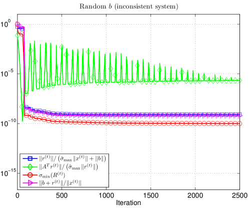
Figure 6.5: Running LSQR with an inconsistent right-hand-side $b$.

The results, presented in Figure 6.5, indicate that there is no good way to decide when to terminate LSQR when used in this way to estimate $\sigma_{\min}$. We obviously cannot rely on the residual approaching $\epsilon_{\text{m}}$, because the problem is inconsistent. The original LSQR paper [30] suggests another stopping condition,

$$\frac{\left\|A^{T}r^{(t)}\right\|}{\hat{\sigma}_{\max}\left\|r^{(t)}\right\|}\leq c\;,$$

but our experiment shows that this ratio may fail to get close to $\epsilon_{\text{m}}$. In our experiment the best local minimum is around $10^{-10}$, six orders of magnitude larger than $\epsilon_{\text{m}}$. Moreover, at that local minimum, around iteration 60, the estimate $\|b+r^{(t)}\|/\|x^{(t)}\|$ is still near $1$, very far from $\sigma_{\min}$. The Lanczos estimate $\sigma_{\min}(R^{(t)})$ is also very inaccurate at that time. There does not appear to be a good way to decide when to stop the iterations and to report the best estimate seen so far.

On matrices with this singular value distribution, our method detects convergence after 2400-2500 iterations, returning a certified estimate of $\sigma_{\min}$ that is accurate to within 15–40% (the accuracy of the Lanczos estimate is better, with relative errors smaller than 10%). Figure 6.6 shows a typical run. The number of iterations is large, but the stopping criteria are robust.

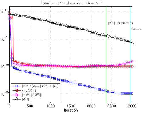
Figure 6.6: Running our method on the same matrix as in Figure 6.5.

In Figure 6.7 all the singular values are distributed linearly from $10^{-8}$ up to $1$ (the dimensions of all matrices in this subsection are again $1000$-by-$400$). Convergence is fairly slow. The gap between $\sigma_{\min}=\sigma_{400}=10^{-8}$ and $\sigma_{399}$ is relatively large, around $\frac{1}{400}$, so $\sigma_{\min}$ is computed accurately.

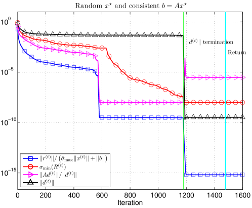
Figure 6.7: Singular values are distributed linearly from $10^{-8}$ up to $1$.

When many singular values are distributed logarithmically or nearly so, convergence is very slow and the small relative gap between $\sigma_{\min}$ and the next-larger singular values causes the method to return a less accurate estimate.

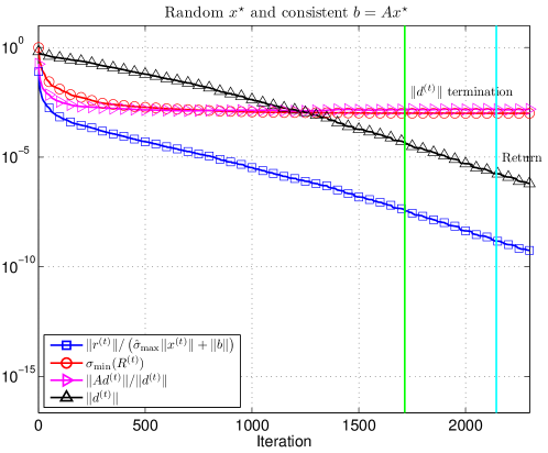
Figure 6.8: 200 singular values are distributed logarithmically from $10^{-3}$ up to $1$, and the rest are equal to $1$.

Figure 6.8 plots the convergence when 200 singular values are distributed logarithmically between $10^{-3}$ and $1$ and the rest are at $1$. We do not see a period of stagnation during which the error is a good estimate of $v_{\min}$. The certified estimate is only accurate to within 31% and the Lanczos estimate to within 10% (much worse than when the smallest singular value is well separated from the rest).

LSQR might have several periods of stagnation. This happens when the spectrum contains several well-separated clusters. Figure 6.9 plots the convergence when the matrix has a multiple singular value at $10^{-10}$, a multiple singular value at $10^{-7}$ (both with multiplicity 10), 300 singular values that are distributed logarithmically between $10^{-3}$ and $10^{-2}$, and the rest are at $1$. We see multiple stagnation periods of both the residual, the error, the Lanczos estimate, and our certified estimate.

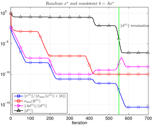
Figure 6.9: 200 singular values are distributed logarithmically from $10^{-3}$ up to $1$, and the rest are equal to $1$.

6.2 Experiments on Large Structured Random Matrices

The next set of experiments was performed on sparse matrices that motivated this project. These matrices have exactly three nonzeros per column, where the location of the nonzeros is random and uniform and their values are $+1$ or $-1$ with equal independent probabilities. This type of matrices arises when simulating the evolution of random 2-dimensional complexes in various stochastic models [1]. Such $m$-by-$n$ matrices tend to be well conditioned when $n<0.9m$ and rank deficient when $n>0.95m$.

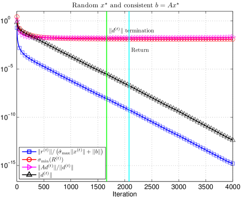
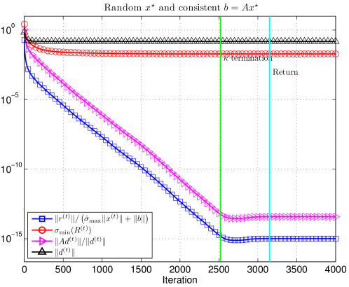
Figure 6.10: Random matrices with 3 nonzeros per row. On the top we see the convergence on a $100{,}000$-by-$90{,}000$ matrix and on the bottom convergence on a $100{,}000$-by-$95{,}000$ matrix.

Figure 6.10 shows that the method converges quite quickly even on large matrices in both the well conditioned and the rank deficient cases. On smaller matrices of this type we were able to assess the accuracy of the method. For $m=1000$, on $n=900$ the algorithm yielded a relative error of 22% (the Lanczos estimate was off by 78%), and on $n=450$ the algorithm yielded a relative error of 41% (the Lanczos estimate was off by 18%). Problems of this type of size $m=1{,}000{,}000$ required similar number of iterations and were easily solved on a laptop. It is worth noting that due to the random structure of the non-zero pattern, it is likely that factorization based condition number estimators will be very slow when applied to this type of matrices.

6.3 Experiments on Many Real-World Matrices

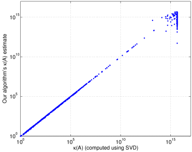
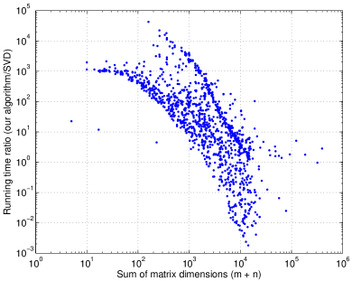
Figure 6.11: Correlation between the actual condition number and the one that we obtain from our algorithm when it converges (left) and the computational cost of our method (implemented in Matlab), relative to the dense SVD, as a function of matrix size (right).

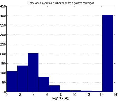
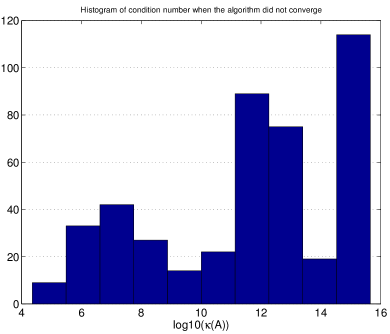
Figure 6.12: Histogram of the condition number of matrices on which our algorithm converged (left) and did not converge (right).

We ran both a dense SVD and our method on all the matrices from Tim Davis’s sparse matrix collection [8] for which $mn^{2}<256\times 10^{9}$. Our method converged in 100,000 iterations or less on 1024 out of the 1468 matrices in this category.

Out of the 1468 matrices, 404 had condition number $1/(64\cdot\epsilon_{\text{m}})\approx 7\times 10^{13}$ or larger. Our method converged on 278 out of them, delivering condition number estimates of $5\times 10^{11}$ or larger. In other words, on all the matrices that were close to rank deficiency, our method detected that the condition number is large, but in some cases it underestimated the actual condition number.

On matrices with condition number smaller than $64/\epsilon_{\text{m}}$, our method always estimated the condition number to within a relative error of 24% or less. Figure 6.11 shows a scatter plot of the condition number reported by our method when it converged vs. the condition number reported by Matlab’s dense SVD.

We ran the method again on some of the matrices on which it failed to converge in 100,000 iterations, allowing the method to run longer. It converged in all cases. For example, on nos1, the method detected convergence after 169,791 iterations. The $\sigma_{\min}$ estimate it returned was actually from iteration 90,173, meaning that at iteration 100,000 it actually converged, but the algorithm was not yet able to detect convergence. We note that nos1 is a square matrix of dimension 237; the method can be slow even on small matrices. Figure 6.12 presents histograms of the dense-SVD condition-numbers of matrices on which our method converged or did not converge. The histograms show that our method can fail to converge (in 100,000 iterations) on both well condition and ill conditioned matrices. It also appears that full-rank ill conditioned matrices are more likely to cause our method difficulties than either well conditioned or rank deficient matrices.

We remark the one clearly sees the effect of inexact arithmetic in these experiments. Since LSQR on an $m$-by-$n$ matrix is equivalent to CG on an $n$-by-$n$ matrix, with exact arithmetic our method’s iteration count should never exceed the dimension. In practice, we see that the number of iterations may well exceed the dimension (e.g., the nos1 matrix). This is because of loss of orthogonality due to floating point rounding.

The running time of our method obviously varies a lot and is not easy to characterize. But on large matrices it is often much faster than a dense SVD, as shown in Figure 6.11.

6.4 Experiments on Large Real-World Matrices

We ran the algorithm on a few very large matrices from the same matrix collection. As on the smaller matrices, the method sometimes converged, although sometimes it exceeded the maximal number of iterations (up to 1,000,000). Table 1 shows a sample of the the statistics of successful runs; they indicate that when the singular spectrum is clustered, the method works well even on very large matrices.

			condest			irlba		PRIMME
	$m$	$n$	time (s)	it. (#mv)	$\kappa$ (est.)	#mv	$\kappa$ (est.)	#mv	$\kappa$ (est.)
rajat10	30202	30202	3.7	3017 (6634)	1.1e+03	43016	1.3e+03	5248	1.3e+03
flower_7_4	67593	27693	0.6	129 (858)	1.5e+01	104	2.0e+01	402	1.9e+01
flower_8_4	125361	55081	3.2	648 (1896)	2.8e+13	4584	2.4e+16	3556	3.7e+00
wheel_601	902103	723605	358	5260	1.3e+14	FAIL		FAIL
Franz11	47104	30144	0.3	73 (746)	$\infty$	712	3.3e+16	528	4.9e+00
lp_ken_18	154699	105127	10	2234 (5068)	2.5e+14	169096	5.7e+16	24832	6.5e+02
lp_pds_20	108175	33874	3.3	848 (2296)	1.4e+14	7304	2.8e+16	6178	6.8e+00
cage15	5154859	5154859	162	73 (746)	1.1e+01	72	1.2e+01	92	1.2e+01
atmosmodl	1489752	1489752	663	6699 (13998)	8.5e+02	662536	1.1e+03	15546	1.1e+03
Rucci1	1977885	109900	2194	20576 (41752)	6.5e+03	1728264	6.8e+03	28604	6.8e+03
LargeRegFile	2111154	801374	146	1304 (3208)	1.0e+04	21032	1.1e+04	4886	1.1e+04
sls	1748122	62729	119	848 (2296)	9.7e+02	8296	1.3e+03	3218	1.3e+03

Table 1: Large real-world matrices whose condition number was successfully computed by our method. Matrices with an underline indicate a structurally rank deficient matrix, or a matrix indicated in the matrix collection as numerically rank deficient.

We also attempted to approximate the condition number using two singular values solvers: irlba [2] and PRIMME [33]. Both are general purpose singular values solvers, so in order to make a fair comparison with our algorithm (which is designed for condition number estimation) we judiciously chose the stopping criteria. From PRIMME, we use the library’s option to supply a special convergence criteria, and stop the method once the residual has dropped below $10\%$ the current estimate of $\sigma_{\min}$. For irlba, we set the code’s convergence tolerance to $10^{-15}$ when our code detected rank deficiency, and to $1/\kappa_{\text{est }}$ otherwise, where $\kappa_{\text{est }}$ is the condition number estimate obtained using our method (of course, this stopping criteria cannot be used in practice, and we use it only for the sake of empirical evaluation). For both algorithms, we restrict the number of iterations to 100,000. Since the different libraries are implemented in different languages (irlba and our algorithm are implemented in MATLAB, while PRIMME does most of the work in C), we measure only the number of matrix-vector products. For the matrices reported in Table 1, unless the matrix is very well conditioned, our algorithm clearly outperforms irlba. As for PRIMME, when the condition number is not too large, PRIMME tends to require less matrix-vector products. However, PRIMME fails to detect very ill-conditioned matrices.

7 Summary

We have presented an adaptation of LSQR to the estimation of the condition number of matrices.

Our method is yet another tool in the spectral condition-number estimation toolbox. It relies almost solely on matrix-vector multiplications, so it can be applied to very large sparse matrices. It does not require much memory, and it is at least as fast as a single application of un-preconditioned LSQR to solve a least-squares problem. The method never returns an overestimate of the condition number.

In many cases, the method is orders-of-magnitude faster than competing methods, especially if $A$ is large and has no sparse triangular factorization.

However, the performance of the method depends on the distribution of the singular values of $A$, and some distributions lead to very slow convergence. When convergence is slow or non-existent, the method still provides a lower bound on the condition number, but it may be loose. In such cases, methods that are based on orthogonal or triangular factorizations or on preconditioned iterative solvers may be faster.

Our method is primarily based on one known property: that the forward error in LSQR tends to converge to an approximate singular vector associated with $\sigma_{\min}$. This property of LSQR and related Krylov-subspace solvers is normally seen as a deficiency (because it slows down the convergence to the minimizer), but it turns out to be beneficial for condition-number estimation.

We have not explored whether a similar technique can be used in other least-squares Krylov methods, such as LSMR [11], MINRES [28], and MINRES-QLP [6].

Acknowledgments

Most of the work was done while Haim Avron was at IBM T.J. Watson Research Center. We thank Nira Dyn for helpful discussions. Sivan Toledo and Alex Druinsky were supported in part by grant 1045/09 from the Israel Science Foundation (founded by the Israel Academy of Sciences and Humanities) and by grant 2010231 from the US-Israel Binational Science Foundation. Haim Avron acknowledges the support from the XDATA program of the Defense Advanced Research Projects Agency (DARPA), administered through Air Force Research Laboratory contract FA8750-12-C-0323.

References

- [1] Lior Aronshtam, Nathan Linial, Tomasz Łuczak, and Roy Meshulam. Collapsibility and vanishing of top homology in random simplicial complexes. Discrete and Computational Geometry, 49(2):317–334, 2013.
- [2] J. Baglama and L. Reichel. Augmented implicitly restarted lanczos bidiagonalization methods. SIAM Journal on Scientific Computing, 27(1):19–42, 2005.
- [3] James Baglama and Lothar Reichel. An implicitly restarted block Lanczos bidiagonalization method using Leja shifts. BIT Numerical Mathematics, 53(2):285–310, 2013.
- [4] Christian H. Bischof, John G. Lewis, and Daniel J. Pierce. Incremental condition estimation for sparse matrices. SIAM Journal on Matrix Analysis and Applications, 11(4):644–659, 1990.
- [5] X.-W. Chang, C. C. Paige, and D. Titley-Peloquin. Stopping criteria for the iterative solution of linear least squares problems. SIAM Journal on Matrix Analysis and Applications, 31(2):831–852, 2009.
- [6] Sou-Cheng T. Choi, Christopher C. Paige, and Michael A. Saunders. MINRES-QLP: A Krylov subspace method for indefinite or singular symmetric systems. SIAM Journal on Scientific Computing, 33(4):1810–1836, 2011.
- [7] Jane K. Cullum and Ralph A. Willoughby. Lanczos Algorithms for Large Symmetric Eigenvalue Computations: Vol. 1 Theory. Birkhaeuser, Boston, MA, USA, 1985, Reprinted by Society for Industrial and Applied Mathematics, Philadelphia, PA, USA, 2002.
- [8] Timothy A. Davis and Yifan Hu. The University of Florida Sparse Matrix Collection. ACM Transactions on Mathematical Software, 38(1):1:1–1:25, November 2011.
- [9] James W. Demmel. Applied Numerical Linear Algebra. SIAM, 1996.
- [10] V. L. Druskin and L. A. Knizhnerman. Error bounds in the simple Lanczos procedure for computing functions of symmetric matrices and eigenvalues. USSR Computational Mathematics and Mathematical Physics, 31(7):20–30, 1991.
- [11] David Chin-Lung Fong and Michael Saunders. LSMR: An iterative algorithm for sparse least-squares problems. SIAM Journal on Scientific Computing, 33(5):2950–2971, 2011.
- [12] Sarah W. Gaaf and Michiel E. Hochstenbach. Probabilistic bounds for the matrix condition number with extended Lanczos bidiagonalization. SIAM Journal on Scientific Computing, 37(5):S581–S601, 2015.
- [13] Gene H. Golub and Charles F. Van Loan. Matrix Computations. JHU Press, 4th edition, 2013.
- [14] Gene H. Golub and Qiang Ye. An inverse free preconditioned krylov subspace method for symmetric generalized eigenvalue problems. SIAM Journal on Scientific Computing, 24(1):312–334, 2002.
- [15] Craig Gotsman and Sivan Toledo. On the computation of null spaces of sparse rectangular matrices. SIAM Journal on Matrix Analysis and Applications, 30:445–463, 2008.
- [16] N. Halko, P. G. Martinsson, and J. A. Tropp. Finding structure with randomness: Probabilistic algorithms for constructing approximate matrix decompositions. SIAM Review, 53(2):217–288, 2011.
- [17] Nicholas J. Higham. FORTRAN codes for estimating the one-norm of a real or complex matrix, with applications to condition estimation. ACM Transactions on Mathematical Software, 14(4):381–396, December 1988.
- [18] Nicholas J. Higham. Accuracy and Stability of Numerical Algorithms. SIAM, 2nd edition, 2002.
- [19] Nicholas J. Higham and Françoise Tisseur. A block algorithm for matrix 1-norm estimation, with an application to 1-norm pseudospectra. SIAM Journal on Matrix Analysis and Applications, 21(4):1185–1201, 2000.
- [20] Michiel E. Hochstenbach. A Jacobi–Davidson type SVD method. SIAM Journal on Scientific Computing, 23(2):606–628, 2001.
- [21] Zhongxiao Jia. Using cross-product matrices to compute the SVD. Numerical Algorithms, 42(1):31–61, May 2006.
- [22] C. S. Kenney, A. J. Laub, and M. S. Reese. Statistical condition estimation for linear systems. SIAM Journal on Scientific Computing, 19(2):566–583, 1998.
- [23] Philip Klein and Hsueh-I Lu. Efficient approximation algorithms for semidefinite programs arising from MAX CUT and COLORING. In Proceedings of the 28th annual ACM Symposium on Theory of Computing, pages 338–347, 1996.
- [24] E. Kokiopoulou, C. Bekas, and E. Gallopoulos. Computing smallest singular triplets with implicitly restarted Lanczos bidiagonalization. Applied Numerical Mathematics, 49(1):39 – 61, 2004. Numerical Algorithms, Parallelism and Applications.
- [25] J. Kuczyński and H. Woźniakowski. Estimating the largest eigenvalue by the power and Lanczos algorithms with a random start. SIAM Journal on Matrix Analysis and Applications, 13(4):1094–1122, 1992.
- [26] R. B. Lehoucq, D. C. Sorensen, and C. Yang. ARPACK Users’ Guide. SIAM, 1998.
- [27] Qiao Liang and Qiang Ye. Computing singular values of large matrices with an inverse-free preconditioned Krylov subspace method. Electronic Transactions on Numerical Analysis, 42:197–221, 2014.
- [28] C. C. Paige and M. A. Saunders. Solution of sparse indefinite systems of linear equations. SIAM Journal on Numerical Analysis, 12(4):617–629, 1975.
- [29] Christopher C. Paige and Michael A. Saunders. Algorithm 583: LSQR: Sparse linear equations and least squares problems. ACM Transactions on Mathematical Software, 8:195–209, 1982.
- [30] Christopher C. Paige and Michael A. Saunders. LSQR: An algorithm for sparse linear equations and sparse least squares. ACM Transactions on Mathematical Software, 8:43–71, 1982.
- [31] Eugene Vecharynski. Preconditioned Iterative Methods for Linear Systems, Eigenvalue and Singular Value Problems. PhD thesis, University of Colorado Denver, 2010.
- [32] L. Wu and A. Stathopoulos. A preconditioned hybrid SVD method for accurately computing singular triplets of large matrices. SIAM Journal on Scientific Computing, 37(5):S365–S388, 2015.
- [33] Lingfei Wu, Eloy Romero, and Andreas Stathopoulos. PRIMME_SVDS: A high-performance preconditioned SVD solver for accurate large-scale computations. CoRR, abs/1607.01404, 2016.