On the effect of the degeneracy among dark energy parameters

Abstract

The dynamics of scalar fields as dark energy is well approximated by some general relations between the equation of state parameter $w(z)$ and the fraction energy density $\Omega_{\phi}$. Based on the approximation, for slowly-rolling scalar fields, we derived the analytical expressions of $w(z)$ which reduce to the popular Chevallier-Polarski-Linder parametrization with explicit degeneracy relation between $w_{0}$ and $w_{a}$. The models approximate the dynamics of scalar fields well and help eliminate the degeneracies among $w_{a}$, $w_{0}$ and $\Omega_{m0}$. With the explicit degeneracy relations, we test their effects on the constraints of cosmological parameters. We find that: (1) The analytical relations between $w_{0}$ and $w_{a}$ for the two models are consistent with observational data; (2) The degeneracies have little effect on $\Omega_{m0}$; (3) The $1\sigma$ error of $w_{0}$ was reduced about 30% with the degeneracy relations.

1 Introduction

To explain the cosmic acceleration found by the observations of type Ia supernovae (SNe Ia) in 1998 hzsst98 ; scpsn98 , we usually introduce an exotic energy component with negative pressure to the right hand side of Einstein equation. This exotic energy component which contributes about 72% to the total energy density in the universe is dubbed as dark energy. Although the cosmological constant is the simplest candidate for dark energy and is consistent with current observations, other possibilities are also explored due to the many orders of magnitude discrepancy between the theoretical estimation and astronomical observations for the cosmological constant. Currently we still have no idea about the nature of dark energy. In particular, the question whether dark energy is just the cosmological constant remains unanswered. For reviews of dark energy, please see Refs. sahni00 ; peeblesde ; padmanabhande ; copelandde ; Caldwell:2009ix ; Bartelmann:2009te ; limiaode .

One way of studying the nature of dark energy is through the observational data. There are many model-independent studies on the nature of dark energy by using the observational data alam04a ; alam04b ; barger ; clarkson ; corasaniti ; astier ; efstathiou ; gerke ; cooray ; flux1 ; weller01 ; huang ; star ; cai ; lampeitl ; corray9 ; gong10a ; gong10b ; gongcqg10 ; gong11 ; Gong:2011rs ; gongmnras13 ; li11 ; yu11 ; cai11 ; wetterich04 ; cpl1 ; cpl2 ; jbp05 ; zhu . In particular, one usually parameterizes the energy density $\Omega_{\phi}(z)$ or the equation of state parameter $w(z)$ of dark energy. Motivated by the tracking solution track1 ; track2 for a wide class of quintessence quintessence potentials in which the equation of state parameter $w(z)$ varies slowly, Efstathiou approximated $w(z)$ with $w(z)=w_{0}-\alpha\ln(1+z)$ in the redshift range $z<4$ efstathiou . However, the most used parametrization for approximating the dynamics of a wide class of scalar fields is the Chevallier-Polarski-Linder (CPL) parametrization with $w(a)=w_{0}+w_{a}(1-a)$ cpl1 ; cpl2 . Because of the degeneracies among the parameters $\Omega_{m0}$, $w_{0}$ and $w_{a}$ in the model, complementary cosmological observations are needed to break the degeneracies. The measurement on the cosmic microwave background anisotropy, the baryon acoustic oscillation (BAO) measurement and the SNe Ia observations provide complementary data.

On the other hand, a minimally coupled scalar field $\phi$ was often invoked to model the quintessence wetterich88 ; peebles88 ; quintessence , and the phantom phantom . For a scalar field with a nearly flat potential, there exist approximate relations between the equation of state parameter $w=p/\rho$ and the energy density parameter $\Omega_{\phi}$ track1 ; track2 ; Robert2008 ; Robert ; Sourish ; Crittenden:2007yy ; Dutta:2008qn ; Gupta:2009kk ; Chiba:2009nh . As discussed above, the dynamics of scalar fields can be approximated with the CPL parametrization and the generic $w-\Omega_{\phi}$ relations, so we expect that the degeneracies among the parameters $w_{0}$, $w_{a}$ and $\Omega_{\phi 0}$ can be broken. By using the generic $w-\Omega_{\phi}$ relations, we can break the degeneracy between $w(z)$ and $\Omega_{\phi}(z)$. Furthermore, $w(z)$ can be approximated by the CPL parametrization with $w_{a}$ expressed as a function of $w_{0}$ and $\Omega_{\phi 0}$, so the two-parameter parametrization reduces to one-parameter parametrization gong1212 . The CPL parametrization with analytical relations among the model parameters helps tighten the constraints on the model parameters.

In this paper, we derive two particular CPL models with $w_{a}$ proportional to $1+w_{0}$, and study the effects of the degeneracy relations between $w_{a}$ and $w_{0}$ by using the following data: the three year Supernova Legacy Survey (SNLS3) sample of 472 SNe Ia data with systematic errors snls3 ; the BAO measurements from the 6dFGS 6dfgs , the distribution of galaxies in the Sloan Digital Sky Survey (SDSS) wjp and the WiggleZ dark energy survey wigglez ; the seven-year Wilkinson Microwave Anisotropy Probe (WMAP7) data wmap7 ; and the Hubble parameter $H(z)$ data hz2 ; hz1 .

2 CPL parametrization with degenerated $w_{0}$ and $w_{a}$

For a quintessence field, the equation of state parameter $w(z)$ is related with its fractional energy density $\Omega_{\phi}=8\pi G\rho_{\phi}/3H^{2}$ as follows Crittenden:2007yy

$$1+w(z)=\kappa^{2}(\phi)\Omega_{\phi}(z)(1-w(z))^{2}/6,$$ (1)

$$\frac{d\phi}{d\ln a}=-\kappa(\phi)\Omega_{\phi}(z)(1-w(z)),$$ (2)

where $\kappa(\phi)=-3H\dot{\phi}/V(\phi)$. For scalar fields satisfying the slow-roll conditions,

$$(\frac{1}{V}\frac{dV}{d\phi})^{2}\ll 1,\quad\frac{1}{V}\frac{d^{2}V}{d{\phi}^{2}}\ll 1,$$ (3)

the dark energy density $\rho_{\phi}(a)$ is nearly constant and it deviates from the cosmological constant by the order $\int_{a}^{1}(1+w)da/a$. Since $1+w(z)\ll 1$, to the zeroth order approximation, the fractional energy density $\Omega_{\phi}(a)$ can be replaced by the cosmological constant

$$\Omega_{\Lambda}(a)=\left[1+(\Omega_{\phi 0}^{-1}-1)a^{-3}\right]^{-1},$$ (4)

and the dynamics of the potential can be approximated by the linear expansion of $\kappa(\phi)$ as $\kappa(\phi)=\kappa_{0}+\kappa_{1}(\phi-\phi_{0})$ Crittenden:2007yy . With these approximations, $w(a)$ was derived as Crittenden:2007yy

$$w(a)=-1+\frac{2}{3}\kappa_{0}^{2}\Omega_{\Lambda}(a)\left[\frac{\Omega_{\Lambda}(a)}{a^{3}\Omega_{\phi 0}}\right]^{2\kappa_{1}/3}.$$ (5)

On the other hand, $w(z)=\gamma-1$ also satisfies the relation Robert2008

$$\frac{d\gamma}{d\Omega_{\phi}}=\frac{-3\gamma(2-\gamma)+\lambda(2-\gamma)\sqrt{3\gamma\Omega_{\phi}}}{3(1-\gamma)\Omega_{\phi}(1-\Omega_{\phi})},$$ (6)

where $\lambda(\phi)=-V^{-1}(\phi)dV(\phi)/d\phi$. For slow-roll scalar fields, $\gamma\ll 1$ and $\lambda$ is almost constant. Assume that $\lambda(\phi)=\lambda(\phi)_{\phi=\phi_{0}}=\lambda_{0}$, a general relationship between $w$ and the energy density $\Omega_{\phi}$ for both quintessence and phantom models was found Robert2008 ; Robert ; Ali:2009mr ,

$$1+w=(1+w_{0})\left[\frac{1}{\sqrt{\Omega_{\phi}}}-\left(\frac{1}{\Omega_{\phi}}-1\right)\tanh^{-1}(\sqrt{\Omega_{\phi}})\right]^{2}$$

$$\times\left[\frac{1}{\sqrt{\Omega_{\phi 0}}}-(\Omega_{\phi 0}^{-1}-1)\tanh^{-1}\sqrt{\Omega_{\phi 0}}\right]^{-2}.$$ (7)

Note that the above result holds for thawing models Caldwell:2005tm with the potentials satisfying the slow roll conditions (3). It does depend on the specific form of the potential $V(\phi)$, furthermore, it also approximates the dynamics of tachyon fields Ali:2009mr ; Chen:2013vba . When $w$ is close to $-1$, to the zeroth order, the fractional energy density $\Omega_{\phi}$ can be approximated by the cosmological constant $\Omega_{\Lambda}$ Crittenden:2007yy ; Robert2008 ; Robert , so

$$w(a)=-1+(1+w_{0})\left[\frac{1}{\sqrt{\Omega_{\phi 0}}}-(\Omega_{\phi 0}^{-1}-1)\tanh^{-1}\sqrt{\Omega_{\phi 0}}\right]^{-2}$$

$$\times\left[\sqrt{1+(\Omega_{\phi 0}^{-1}-1)a^{-3}}-(\Omega_{\phi 0}^{-1}-1)a^{-3}\tanh^{-1}[1+(\Omega_{\phi 0}^{-1}-1)a^{-3}]^{-1/2}\right]^{2}.$$ (8)

In Ref. Robert2008 , it was explicitly shown in the Fig. 4 that the analytical result (2) fits $w(a)$ well for thawing quintessence models with the potentials $V(\phi)\sim\phi^{2}$, $V(\phi)\sim\phi^{-2}$, and $V(\phi)\sim\exp(-\lambda\phi)$. In Ref. Robert , it was explicitly shown in the Fig. 1 that the analytical result (2) gives the behavior of $w(a)$ for thawing phantom models with the potentials $V(\phi)\sim\phi^{6}$, $V(\phi)\sim\phi^{2}$, $V(\phi)\sim\phi^{-2}$, and $V(\phi)\sim\exp(-\lambda\phi)$. Therefore, we can use $w(a)$ given by equation (2) to approximate thawing scalar fields. If we Taylor expand $\Omega_{\phi}(a)$ and $w(a)$ around $a=1$, we get

$$\Omega_{\phi}\approx\Omega_{\phi 0}[1-3(1-\Omega_{\phi 0})(1-a)],$$ (9)

and

$$w=w_{0}+6(1+w_{0})\frac{\Omega_{\phi 0}^{-1/2}-\sqrt{\Omega_{\phi 0}}-(\Omega_{\phi 0}^{-1}-1)\tanh^{-1}(\sqrt{\Omega_{\phi 0}})}{\Omega_{\phi 0}^{-1/2}-(\Omega_{\phi 0}^{-1}-1)\tanh^{-1}(\sqrt{\Omega_{\phi 0}})}(1-a).$$ (10)

Therefore, we derive the CPL parametrization with $w_{a}$ determined by $w_{0}$ and $\Omega_{\phi 0}$ starting from equation (2). We call this model as SSLCPL model. In particular, we get gong1212 ; Chen:2013vba

$$w_{a}=6(1+w_{0})\frac{(\Omega_{\phi 0}^{-1}-1)[\sqrt{\Omega_{\phi 0}}-\tanh^{-1}(\sqrt{\Omega_{\phi 0}})]}{\Omega_{\phi 0}^{-1/2}-(\Omega_{\phi 0}^{-1}-1)\tanh^{-1}(\sqrt{\Omega_{\phi 0}})}.$$ (11)

When $\Omega_{\phi 0}=0.7$, we get $w_{a}=-1.42(1+w_{0})$ which is consistent with the numerical result $w\approx w_{0}-1.5(1+w_{0})(1-a)$ obtained in Robert2008 ; Robert . Note that we derived the analytical expression of $w_{a}$ within the CPL parametrization which captures the main dynamics of thawing scalar fields, this expression is not just a phenomenological dark energy parametrization, it actually approximates the dynamics of thawing scalar fields. For the SSLCPL model, we only have two model parameters $\Omega_{m0}$ and $w_{0}$ for the spatially flat case. To see how well the approximation performs, in Fig. 1, we show the evolutions of $w(a)$ for the power-law potentials $V(\phi)\sim\phi^{5}$ and $V(\phi)\sim\phi^{-5}$, and the approximations (2) and (10). It is clear that the relative error brought by the approximation is under a few percent. For the power-law potential $V(\phi)\sim\phi^{n}$ with other numbers of power $n$, the relative error is also a few percent.

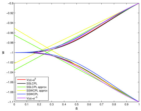
Figure 1: The evolutions of $w(a)$ for the potentials $V(\phi)\sim\phi^{5}$ and $V(\phi)\sim\phi^{-5}$, the SSLCPL model (2) and (10) and SSWCPL model (2) and (16). The initial conditions are taken as $\Omega_{\phi 0}=0.72$ and $w_{0}=-0.9$ for the quintessence and $w_{0}=-1.1$ for the phantom.

From the evolution equation satisfied by $\Omega_{\phi}$,

$$\Omega^{\prime}_{\phi}=-3w\Omega_{\phi}(1-\Omega_{\phi}),$$ (12)

we take the approximate solution for $\Omega_{\phi}$ with constant equation of state $w=w_{0}$,

$$\Omega_{w}=\frac{\Omega_{\phi 0}a^{-3w}}{1-\Omega_{\phi 0}+\Omega_{\phi 0}a^{-3w}},$$ (13)

so

$$w(a)=-1+(1+w_{0})\left[\frac{1}{\sqrt{\Omega_{\phi 0}}}-(\Omega_{\phi 0}^{-1}-1)\tanh^{-1}\sqrt{\Omega_{\phi 0}}\right]^{-2}$$

$$\times\left[\sqrt{1+(\Omega_{\phi 0}^{-1}-1)a^{3w}}-(\Omega_{\phi 0}^{-1}-1)a^{3w}\tanh^{-1}[1+(\Omega_{\phi 0}^{-1}-1)a^{3w}]^{-1/2}\right]^{2}.$$ (14)

Then Taylor expansion $\Omega_{\phi}(a)$ around $a=1$ gives

$$\Omega_{\phi}=\{1+(\Omega_{\phi 0}^{-1}-1)[1-3w(1-a)]\}^{-1}.$$ (15)

Substituting Eq. (15) into Eq. (2), we obtain,

$$w(a)=w_{0}-6w_{0}(1+w_{0})\frac{(\Omega_{\phi 0}^{-1}-1)[\sqrt{\Omega_{\phi 0}}-\tanh^{-1}(\sqrt{\Omega_{\phi 0}})](1-a)}{\Omega_{\phi 0}^{-1/2}-(\Omega_{\phi 0}^{-1}-1)\tanh^{-1}(\sqrt{\Omega_{\phi 0}})},$$ (16)

so again we get CPL parametrization with

$$w_{a}=-6w_{0}(1+w_{0})\frac{(\Omega_{\phi 0}^{-1}-1)[\sqrt{\Omega_{\phi 0}}-\tanh^{-1}(\sqrt{\Omega_{\phi 0}})]}{\Omega_{\phi 0}^{-1/2}-(\Omega_{\phi 0}^{-1}-1)\tanh^{-1}(\sqrt{\Omega_{\phi 0}})}.$$ (17)

We call this model as SSWCPL model. For the SSWCPL model, we only have two model parameters $\Omega_{m0}$ and $w_{0}$ for the spatially flat case. In Fig. 1, we show the evolutions of $w(a)$ for the approximation (2) and (16). It is clear that the relative errors brought by the approximations are under a few percent. Contrary to the intuition that the approximation with $\Omega_{w}$ may be inappropriate, the numerical results show that the relative error brought by the approximation is still small, so it is a good approximation. For both the SSLCPL and SSWCPL models, we find that $w_{a}\propto 1+w_{0}$, so the models are automatically consistent with $\Lambda$CDM model with $w_{0}=-1$ and $w_{a}=0$. We would like to emphasize that the models we proposed well approximate the dynamics of a wide class of thawing scalar fields in the whole redshift region as shown in Fig. 1, they are different from both $\Lambda$CDM and $w$CDM model which cannot approximate dynamical scalar fields, and they eliminate the degeneracy between $w_{0}$ and $w_{a}$ for the CPL parametrization. Although the CPL parametrization remains to be a good approximation for the dynamics of a wide class of scalar fields at low redshifts, the degeneracy among the model parameters is still a problem for the fitting of cosmological data, our models break the degeneracy and help tighten the constraints on cosmological models.

3 Observational constraints

We apply the SNe Ia, BAO, WMAP7 and the Hubble parameter $H(z)$ data to test the effects of the degeneracy relations (11) and (17) on the constraints of $\Omega_{m0}$ and $w_{0}$. The SNLS3 SNe Ia data consists of 123 low-redshift SNe Ia data with $z<0.1$ mainly from Calan/Tololo, CfAI, CfAII, CfAIII and CSP, 242 SNe Ia data over the redshift range $0.08<z<1.06$ observed from the SNLS snls3 , 93 intermediate-redshift SNe Ia data with $0.06<z<0.4$ observed during the first season of SDSS-II supernova survey sdss2 , and 14 high-redshift SNe Ia data with $z>0.8$ from Hubble Space Telescope riessgold . For the fitting to the SNLS3 data, we need to add two more nuisance parameters $\alpha$ and $\beta$.

The BAO data wigglez consists of the measurement at the redshift $z=0.106$ from the 6dFGS 6dfgs , the measurements of the distribution of galaxies at two redshifts $z=0.2$ and $z=0.35$ wjp in the SDSS and the measurements of the acoustic parameter at three redshifts $z=0.44$, $z=0.6$ and $z=0.73$ from WiggleZ dark energy survey wigglez . For the BAO data, we need to add two more nuisance parameters $\Omega_{b}h^{2}$ and $\Omega_{m}h^{2}$.

For the WMAP7 data, we use the measurements of the shift parameter and the acoustic index at the recombination redshift wmap7 , and we need to add two more nuisance parameters $\Omega_{b}h^{2}$ and $\Omega_{m}h^{2}$.

The Hubble parameter $H(z)$ data consists of the measurements of $H(z)$ at 11 different redshifts obtained from the differential ages of passively evolving galaxies hz1a ; hz1 , and three data points at redshifts $z=0.24$, $z=0.34$ and $z=0.43$, determined by taking the BAO scale as a standard ruler in the radial direction hz2 . The $H(z)$ data spans out to the redshift regions $z=1.75$.

After obtaining the constraints on the model parameters, we reconstruct $w(z)$ and apply the $Om$ diagnostic omztest to detect the deviation from the $\Lambda$CDM model. $Om(z)$ is defined as

$$Om(z)=\frac{E^{2}(z)-1}{(1+z)^{3}-1},$$ (18)

where the dimensionless Hubble parameter $E(z)=H(z)/H(z=0)$.

Now we consider the effects of the degeneracy relations (11) and (17) on $\Omega_{m0}$ and $w_{0}$ for the spatially flat case $\Omega_{k0}=0$. Fitting the SSLCPL model to the observational data, we get the marginalized $1\sigma$ constraints $\Omega_{m0}=0.275^{+0.015}_{-0.011}$ and $w_{0}=-1.08^{+0.11}_{-0.09}$ with $\chi^{2}=432.6$. By using the degeneracy relation (11) and the correlation between $\Omega_{m0}$ and $w_{0}$, we derived the marginalized $1\sigma$ constraint $w_{a}=0.11^{+0.12}_{-0.14}$. We show the marginalized $1\sigma$ and $2\sigma$ contours of $\Omega_{m0}$ and $w_{0}$, and $w_{0}$ and $w_{a}$ in Fig. 2. By using the correlation between $\Omega_{m0}$ and $w_{0}$, we reconstruct the evolutions of $w(z)$ and $Om(z)$ in Fig. 2.

Fitting the SSWCPL model to the observational data, we get the marginalized $1\sigma$ constraints $\Omega_{m0}=0.276^{+0.014}_{-0.013}$ and $w_{0}=-1.09\pm 0.10$ with $\chi^{2}=432.6$. By using the degeneracy relation (17) and the correlation between $\Omega_{m0}$ and $w_{0}$, we derived the marginalized $1\sigma$ constraint $w_{a}=0.12^{+0.16}_{-0.15}$. We show the marginalized $1\sigma$ and $2\sigma$ contours of $\Omega_{m0}$ and $w_{0}$, and $w_{0}$ and $w_{a}$ in Fig. 3. By using the correlation between $\Omega_{m0}$ and $w_{0}$, we reconstruct the evolutions of $w(z)$ and $Om(z)$ in Fig. 3.

Fitting the CPL model to the observational data, we get the marginalized $1\sigma$ constraints $\Omega_{m0}=0.278^{+0.018}_{-0.011}$, $w_{0}=-1.0^{+0.17}_{-0.13}$ and $w_{a}=-0.33_{-1.03}^{+0.53}$ with $\chi^{2}=432.4$. We show the marginalized $1\sigma$ and $2\sigma$ contours of $\Omega_{m0}$ and $w_{0}$, and $w_{0}$ and $w_{a}$ in Fig. 4. By using the correlations among the parameters, we reconstruct the evolutions of $w(z)$ and $Om(z)$ in Fig. 4. These results are summarized in Table 1.

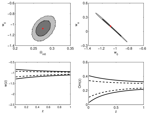
Figure 2: The marginalized $1\sigma$ and $2\sigma$ constraints on the flat SSLCPL model. The upper panels are for the $1\sigma$ and $2\sigma$ contour plots of $\Omega_{m0}-w_{0}$ and $w_{0}-w_{a}$. The lower panels show the reconstructions of $w(z)$ and $Om(z)$ by using the constraints on $\Omega_{m0}$ and $w_{0}$.

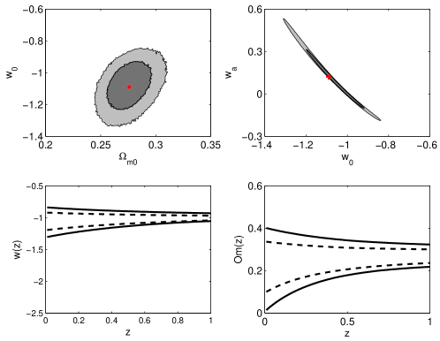
Figure 3: The marginalized $1\sigma$ and $2\sigma$ constraints on the flat SSWCPL model. The upper panels are for the $1\sigma$ and $2\sigma$ contour plots of $\Omega_{m0}-w_{0}$ and $w_{0}-w_{a}$. The lower panels show the reconstructions of $w(z)$ and $Om(z)$ by using the constraints on $\Omega_{m0}$ and $w_{0}$.

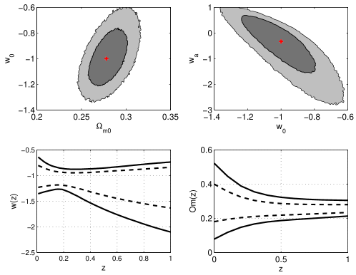
Figure 4: The marginalized $1\sigma$ and $2\sigma$ constraints on the flat CPL model. The upper panels are for the $1\sigma$ and $2\sigma$ contour plots of $\Omega_{m0}-w_{0}$ and $w_{0}-w_{a}$. The lower panels are the reconstructions of $w(z)$ and $Om(z)$ by using the constraints on $\Omega_{m0}$, $w_{0}$ and $w_{a}$.

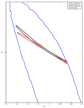
Figure 5: The marginalized $2\sigma$ contours of $w_{0}$ and $w_{a}$ for the SSLCPL, SSWCPL and CPL models.

Before comparing the constraints for the SSLCPL and SSWCPL models with the familiar CPL model, we need to check the consistencies of the degeneracy relations (11) and (17). So we put the $2\sigma$ contour plots of $w_{0}$ and $w_{a}$ from Figs. 2-4 together in Fig. 5, we see that the analytical degeneracies (11) for the SSLCPL model and (17) for the SSWCPL model are consistent with the $w_{0}-w_{a}$ contour for the CPL model obtained from the observational constraints, and the variation of $w(z)$ ($w_{a}$) is constrained much tighter with the help of analytical relations (11) and (17). The effects of the degeneracy relations (11) and (17) on $\Omega_{m0}$ are minimal. The $1\sigma$ errors of $w_{0}$ for SSLCPL and SSWCPL models are reduced around 30% with the degeneracy relations (11) and (17) compared with that in CPL model. Comparing the results from the three models, we find that all three models fit the observational data well because they give almost the same value of $\chi^{2}$. In terms of the Akaike information criterion (AIC) aic or Bayesian information criterion (BIC) bic , the SSLCPL and SSWCPL model fit the observational data a little better than the CPL model does. All three models are consistent with $\Lambda$CDM model at the $1\sigma$ level, as shown explicitly by the $w(z)$ and $Om(z)$ plots in Figs. 2-4.

With the constraints on the model parameters $\Omega_{m0}$ and $w_{0}$, we can get the constraints on the forms of the thawing potential $V(\phi)$ by using the following relations,

$$\left(\frac{d\phi}{d\ln a}\right)^{2}=3m^{2}_{pl}\Omega_{\phi}(a)|1+w(a)|,$$ (19)

$$V(a)=\frac{1}{2}\rho_{cr0}(1-w(a))\Omega_{\phi}(a)(H(a)/H_{0})^{2},$$ (20)

where $m_{pl}=(8\pi G)^{-1/2}$ and the current critical density $\rho_{cr0}=3m^{2}_{pl}H_{0}^{2}$. The allowed $1\sigma$ regions of the thawing potentials for the phantom and quintessence cases are shown in Fig. 6. For the phantom case, the scalar field climbs up the potential, the potential $V(\phi)=\phi^{0.85}$ shown with the dashed line is inside the allowed $1\sigma$ region. For the quintessence case, the scalar field rolls down the potential, the potential $V(\phi)=\phi$ shown with the dashed line is inside the allowed $1\sigma$ region.

Table 1: The marginalized $1\sigma$ constraints from observational data.

Model	$\Omega_{m}$	$w_{0}$	$w_{a}$
flat SSLCPL	$0.275^{+0.015}_{-0.011}$	$-1.08^{+0.11}_{-0.09}$	$0.11^{+0.12}_{-0.14}$
flat SSWCPL	$0.276^{+0.014}_{-0.013}$	$-1.09\pm 0.10$	$0.12^{+0.16}_{-0.15}$
flat CPL	$0.278^{+0.018}_{-0.011}$	$-1.0^{+0.17}_{-0.13}$	$-0.33_{-1.03}^{+0.53}$

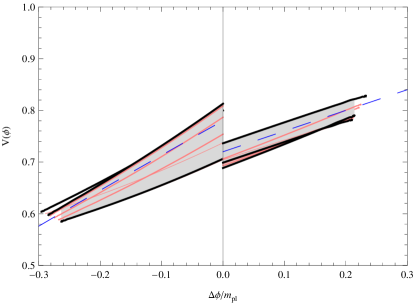
Figure 6: The $1\sigma$ constraint on the thawing potential. The left side if for the phantom field and the right side is for the quintessence field. The potential is in the unit of the current critical density $\rho_{cr0}$ and $\Delta\phi$ is the difference between the scalar field $\phi$ and its current value $\phi_{0}$. The dashed lines show the potential $V(\phi)=\phi^{0.85}$ for the phantom case and $V(\phi)=\phi$ for the quintessence case.

4 Conclusions

From the relationship (2) for thawing models with a nearly flat potential and the CPL approximation for a wide class of dynamical dark energy models, we derived the SSLCPL and SSWCPL models which break the degeneracies among $\Omega_{\phi 0}$, $w_{0}$ and $w_{a}$. The two models reduce to the CPL model with only one free parameter $w_{0}$. The relative errors on the equation of state brought by the SSLCPL and SSWCPL approximations are under a few percent, so these models capture the main dynamics of the thawing model and approximate the dynamics of a wide class of thawing models well. Instead of studying a particular dynamical dark energy model, the SSLCPL and SSWCPL models can be used to probe the general properties of dynamical dark energy. The proposed degeneracy relations for $w_{0}$ and $w_{a}$ are consistent with that found for the familiar CPL model, so the SSLCPL and SSWCPL models are self-consistent. Current observational data constrain the current value of the equation of state $w_{0}$ of dark energy around $-1$ with more than 10% error. The current value of the variation of the equation of state $w_{a}$ is loosely constrained; with the relation between $w_{0}$ and $w_{a}$ which is proportional to $1+w_{0}$ found in SSLCPL and SSWCPL models, $w_{a}$ is tightly constrained and $w_{0}\leq-1$ at the $1\sigma$ level. Both models give almost the same minimum $\chi^{2}$ as the original CPL does when fitting to the observational data. In terms of AIC or BIC, the models fit the observational data a litter better than the original CPL does. With the help of relations (11) and (17), the $1\sigma$ error bar of $w_{0}$ is reduced about 30%. The result is almost the same when we replace the WMAP7 data by the Planck data planck13 ; wangyun13 ; Gao:2013pfa . Both SSLCPL and SSWCPL models have only one free parameter and they help tighten the constraint on the property of dark energy.

With the tighter constraints on the parameters $\Omega_{m0}$ and $w_{0}$, we obtain the constraints on the thawing potential $V(\phi)$. For the phantom case, the potential $V(\phi)=\phi^{0.85}$ is consistent with current observations. For the quintessence case, the potential $V(\phi)=\phi$ is consistent with current observations.

- (1) A.G. Riess, et al., Astron. J. 116, 1009 (1998). DOI 10.1086/300499
- (2) S. Perlmutter, et al., Astrophys. J. 517, 565 (1999). DOI 10.1086/307221
- (3) V. Sahni, A.A. Starobinsky, Int. J. Mod. Phys. D 9, 373 (2000)
- (4) P. Peebles, B. Ratra, Rev. Mod. Phys. 75, 559 (2003). DOI 10.1103/RevModPhys.75.559
- (5) T. Padmanabhan, Phys. Rept. 380, 235 (2003). DOI 10.1016/S0370-1573(03)00120-0
- (6) E.J. Copeland, M. Sami, S. Tsujikawa, Int. J. Mod. Phys. D. 15, 1753 (2006). DOI 10.1142/S021827180600942X
- (7) R.R. Caldwell, M. Kamionkowski, Ann. Rev. Nucl. Part. Sci. 59, 397 (2009). DOI 10.1146/annurev-nucl-010709-151330
- (8) M. Bartelmann, Rev. Mod. Phys. 82, 331 (2010). DOI 10.1103/RevModPhys.82.331
- (9) M. Li, X.D. Li, S. Wang, Y. Wang, Commun. Theor. Phys. 56, 525 (2011). DOI 10.1088/0253-6102/56/3/24
- (10) U. Alam, V. Sahni, T.D. Saini, A. Starobinsky, Mon. Not. Roy. Astron. Soc. 354, 275 (2004). DOI 10.1111/j.1365-2966.2004.08189.x
- (11) U. Alam, V. Sahni, A. Starobinsky, JCAP 0406, 008 (2004). DOI 10.1088/1475-7516/2004/06/008
- (12) V. Barger, Y. Gao, D. Marfatia, Phys. Lett. B 648, 127 (2007). DOI 10.1016/j.physletb.2007.03.021
- (13) C. Clarkson, M. Cortes, B.A. Bassett, JCAP 0708, 011 (2007). DOI 10.1088/1475-7516/2007/08/011
- (14) P.S. Corasaniti, E. Copeland, Phys. Rev. D 67, 063521 (2003). DOI 10.1103/PhysRevD.67.063521
- (15) P. Astier, Phys. Lett. B 500, 8 (2001). DOI 10.1016/S0370-2693(01)00072-7
- (16) G. Efstathiou, Mon. Not. Roy. Astron. Soc. 310, 842 (1999). DOI 10.1046/j.1365-8711.1999.02997.x
- (17) B.F. Gerke, G. Efstathiou, Mon. Not. Roy. Astron. Soc. 335, 33 (2002). DOI 10.1046/j.1365-8711.2002.05612.x
- (18) S. Sullivan, A. Cooray, D.E. Holz, JCAP 0709, 004 (2007). DOI 10.1088/1475-7516/2007/09/004
- (19) Y. Wang, P. Mukherjee, Astrophys. J. 606, 654 (2004). DOI 10.1086/383196
- (20) J. Weller, A. Albrecht, Phys. Rev. Lett. 86, 1939 (2001). DOI 10.1103/PhysRevLett.86.1939
- (21) Q.G. Huang, M. Li, X.D. Li, S. Wang, Phys. Rev. D. 80, 083515 (2009). DOI 10.1103/PhysRevD.80.083515
- (22) A. Shafieloo, V. Sahni, A.A. Starobinsky, Phys. Rev. D. 80, 101301 (2009). DOI 10.1103/PhysRevD.80.101301
- (23) R.G. Cai, Int. J. Mod. Phys. D. 20, 1313 (2011). DOI 10.1142/S0218271811019499
- (24) H. Lampeitl, R. Nichol, H. Seo, T. Giannantonio, C. Shapiro, et al., Mon.Not.Roy.Astron.Soc. 401, 2331 (2009). DOI 10.1111/j.1365-2966.2009.15851.x
- (25) P. Serra, A. Cooray, D.E. Holz, A. Melchiorri, S. Pandolfi, et al., Phys. Rev. D. 80, 121302 (2009). DOI 10.1103/PhysRevD.80.121302
- (26) Y. Gong, R.G. Cai, Y. Chen, Z.H. Zhu, JCAP 1001, 019 (2010). DOI 10.1088/1475-7516/2010/01/019
- (27) Y. Gong, B. Wang, R.g. Cai, JCAP 1004, 019 (2010). DOI 10.1088/1475-7516/2010/04/019
- (28) N. Pan, Y. Gong, Y. Chen, Z.H. Zhu, Class. Quant. Grav. 27, 155015 (2010). DOI 10.1088/0264-9381/27/15/155015
- (29) Y. Gong, X.m. Zhu, Z.H. Zhu, Mon. Not. Roy. Astron. Soc. 415, 1943 (2011). DOI 10.1111/j.1365-2966.2011.18846.x
- (30) Y. Gong, Q. Gao, Z.H. Zhu, Int. J. Mod. Phys. Conf. Ser. 10, 85 (2012). DOI 10.1142/S201019451200579X
- (31) Y. Gong, Q. Gao, Z.H. Zhu, Mon. Not. Roy. Astron. Soc. 430, 3142 (2013). DOI 10.1093/mnras/stt120
- (32) X.D. Li, S. Li, S. Wang, W.S. Zhang, Q.G. Huang, et al., JCAP 1107, 011 (2011). DOI 10.1088/1475-7516/2011/07/011
- (33) Z. Li, P. Wu, H. Yu, Phys. Lett. B 695, 1 (2011). DOI 10.1016/j.physletb.2010.10.044
- (34) Q. Su, Z.L. Tuo, R.G. Cai, Phys. Rev. D 84, 103519 (2011). DOI 10.1103/PhysRevD.84.103519
- (35) C. Wetterich, Phys. Lett. B. 594, 17 (2004). DOI 10.1016/j.physletb.2004.05.008
- (36) M. Chevallier, D. Polarski, Int. J. Mod. Phys. D. 10, 213 (2001). DOI 10.1142/S0218271801000822
- (37) E.V. Linder, Phys. Rev. Lett. 90, 091301 (2003). DOI 10.1103/PhysRevLett.90.091301
- (38) H. Jassal, J. Bagla, T. Padmanabhan, Mon. Not. Roy. Astron. Soc. 356, L11 (2005)
- (39) E. Barboza, J. Alcaniz, Z.H. Zhu, R. Silva, Phys. Rev. D 80, 043521 (2009). DOI 10.1103/PhysRevD.80.043521
- (40) I. Zlatev, L.M. Wang, P.J. Steinhardt, Phys. Rev. Lett. 82, 896 (1999). DOI 10.1103/PhysRevLett.82.896
- (41) P.J. Steinhardt, L.M. Wang, I. Zlatev, Phys. Rev. D 59, 123504 (1999). DOI 10.1103/PhysRevD.59.123504
- (42) R. Caldwell, R. Dave, P.J. Steinhardt, Phys. Rev. Lett. 80, 1582 (1998). DOI 10.1103/PhysRevLett.80.1582
- (43) C. Wetterich, Nucl. Phys. B 302, 668 (1988). DOI 10.1016/0550-3213(88)90193-9
- (44) B. Ratra, P. Peebles, Phys. Rev. D 37, 3406 (1988). DOI 10.1103/PhysRevD.37.3406
- (45) R. Caldwell, Phys. Lett. B 545, 23 (2002). DOI 10.1016/S0370-2693(02)02589-3
- (46) R.J. Scherrer, A. Sen, Phys. Rev. D. 77, 083515 (2008). DOI 10.1103/PhysRevD.77.083515
- (47) R.J. Scherrer, A. Sen, Phys. Rev. D. 78, 067303 (2008). DOI 10.1103/PhysRevD.78.067303
- (48) S. Dutta, R.J. Scherrer, Phys. Lett. B. 704, 265 (2011). DOI 10.1016/j.physletb.2011.09.034
- (49) R. Crittenden, E. Majerotto, F. Piazza, Phys. Rev. Lett. 98, 251301 (2007). DOI 10.1103/PhysRevLett.98.251301
- (50) S. Dutta, R.J. Scherrer, Phys. Rev. D 78, 123525 (2008). DOI 10.1103/PhysRevD.78.123525
- (51) G. Gupta, E.N. Saridakis, A.A. Sen, Phys.Rev. D79, 123013 (2009). DOI 10.1103/PhysRevD.79.123013
- (52) T. Chiba, S. Dutta, R.J. Scherrer, Phys. Rev. D 80, 043517 (2009). DOI 10.1103/PhysRevD.80.043517
- (53) Q. Gao, Y. Gong, Int. J. Mod. Phys. D 22, 1350035 (2013). DOI 10.1142/S0218271813500351
- (54) A. Conley, J. Guy, M. Sullivan, N. Regnault, P. Astier, et al., Astrophys. J. Suppl. 192, 1 (2011). DOI 10.1088/0067-0049/192/1/1
- (55) F. Beutler, C. Blake, M. Colless, D.H. Jones, L. Staveley-Smith, et al., Mon. Not. Roy. Astron. Soc. 416, 3017 (2011). DOI 10.1111/j.1365-2966.2011.19250.x
- (56) W.J. Percival, et al., Mon. Not. Roy. Astron. Soc. 401, 2148 (2010). DOI 10.1111/j.1365-2966.2009.15812.x
- (57) C. Blake, E. Kazin, F. Beutler, T. Davis, D. Parkinson, et al., Mon. Not. Roy. Astron. Soc. 418, 1707 (2011). DOI 10.1111/j.1365-2966.2011.19592.x
- (58) E. Komatsu, et al., Astrophys. J. Suppl. 192, 18 (2011). DOI 10.1088/0067-0049/192/2/18
- (59) E. Gaztanaga, A. Cabre, L. Hui, Mon. Not. Roy. Astron. Soc. 399, 1663 (2009). DOI 10.1111/j.1365-2966.2009.15405.x
- (60) J. Simon, L. Verde, R. Jimenez, Phys. Rev. D. 71, 123001 (2005). DOI 10.1103/PhysRevD.71.123001
- (61) A. Ali, M. Sami, A. Sen, Phys. Rev. D 79, 123501 (2009). DOI 10.1103/PhysRevD.79.123501
- (62) R. Caldwell, E.V. Linder, Phys. Rev. Lett. 95, 141301 (2005). DOI 10.1103/PhysRevLett.95.141301
- (63) X. Chen, Y. Gong, The limit on for tachyon dark energy (2013), arXiv: 1309.2044.
- (64) R. Kessler, A. Becker, D. Cinabro, J. Vanderplas, J.A. Frieman, et al., Astrophys. J. Suppl. 185, 32 (2009). DOI 10.1088/0067-0049/185/1/32
- (65) A.G. Riess, L.G. Strolger, S. Casertano, H.C. Ferguson, B. Mobasher, et al., Astrophys. J. 659, 98 (2007). DOI 10.1086/510378
- (66) D. Stern, R. Jimenez, L. Verde, M. Kamionkowski, S.A. Stanford, JCAP 1002, 008 (2010). DOI 10.1088/1475-7516/2010/02/008
- (67) V. Sahni, A. Shafieloo, A.A. Starobinsky, Phys. Rev. D. 78, 103502 (2008). DOI 10.1103/PhysRevD.78.103502
- (68) H. Akaike, IEEE Transactions on Automatic Control 19, 716 (1974)
- (69) G. Schwarz, Annals of Statistics 6(2), 461 (1978)
- (70) P. Ade, et al., Planck 2013 results. I. Overview of products and scientific results (2013), arXiv: 1303.5062
- (71) Y. Wang, S. Wang, Phys. Rev. D 88, 043522 (2013). DOI 10.1103/PhysRevD.88.043522
- (72) Q. Gao, Y. Gong, The tension on the cosmological parameters from different observational data (2013), arXiv: 1308.5627.