Yarkovsky-driven impact risk analysis for asteroid (99942) Apophis

Abstract

We assess the risk of an Earth impact for asteroid (99942) Apophis by means of a statistical analysis accounting for the uncertainty of both the orbital solution and the Yarkovsky effect. We select those observations with either rigorous uncertainty information provided by the observer or a high established accuracy. For the Yarkovsky effect we perform a Monte Carlo simulation that fully accounts for the uncertainty in the physical characterization, especially for the unknown spin orientation. By mapping the uncertainty information onto the 2029 $b$-plane and identifying the keyholes corresponding to subsequent impacts we assess the impact risk for future encounters. In particular, we find an impact probability greater than 10^-6 for an impact in 2068. We analyze the stability of the impact probability with respect to the assumptions on Apophis’ physical characterization and consider the possible effect of the early 2013 radar apparition.

1 Introduction

Asteroid (99942) Apophis was discovered by R. A. Tucker, D. J. Tholen, and F. Bernardi at Kitt Peak, Arizona on 2004 June 19 (Minor Planet Supplement 109613). Because of its motion, the asteroid was immediately recognized as an object of interest and therefore was observed again on June 20. In the following days, issues related to telescope scheduling, bad weather, and lunar interference made it impossible to collect new observations. By the time the Moon was out of the way, the solar elongation had become too small, thus making the object even more difficult to observe. Thus, the asteroid was lost until December 2004, when it was rediscovered by G. J. Garradd at Siding Springs, Australia (Gilmore et al., 2004). Thanks to the December 2004 observations, Apophis was recognized as a potentially hazardous asteroid, with a peak impact probability (IP) of 2.7% in April 2029 reported by Sentry and NEODyS. Also, the new observations revealed astrometric errors in the discovery observations, for which D. J. Tholen remeasured the positions and adjusted the time (Minor Planet Circulars 53585 and 54280). On 2004 December 27 the Spacewatch survey reported pre-discovery observations (Gleason et al., 2004) from March 2004 that ruled out any impact possibility for 2029.

In January 2005 Apophis was observed by radar from the Arecibo observatory, obtaining three Doppler and two delay measurements. In August 2005 and May 2006 two more Doppler observations were obtained. These observations significantly reduced Apophis orbital uncertainty and led to a 6 Earth radii nominal distance from the geocenter in 2029 (Giorgini et al., 2008). Though the 2029 impact was ruled out, other potential impacts were revealed in the following decades. Moreover, the exceptionally small close approach distance turns a well determined pre-2029 orbit to a poorly known post-2029 orbit for which scattering effects are dominant. Therefore, even small perturbations prior to 2029 play an important role.

Chesley (2006) shows that the Yarkovsky effect (Bottke et al., 2006) substantially affects post-2029 predictions, and therefore has to be taken into account for Apophis impact predictions. Bancelin et al. (2012) also suggest that the Yarkovsky effect is relevant, though they do not account for the corresponding perturbation for their risk assessment. However, the available physical characterization of Apophis is not sufficient to estimate the Yarkovsky effect as was done in the case of asteroid (101955) 1999 RQ₃₆ (Milani et al., 2009; Chesley et al., 2012). In particular the lack of information for spin orientation does not allow one to determine whether the Apophis semimajor axis is drifting inwards or outwards. In some cases, the orbital drift associated with the Yarkovsky effect can be measured from the orbital fit to the observations (Farnocchia et al., 2013). Unluckily, this is not yet possible for Apophis, and upcoming radar observations are unlikely to help in constraining the Yarkovsky effect. Another nongravitational perturbation that could be important is solar radiation pressure. However, Žižka and Vokrouhlický (2011) show that solar radiation pressure has a much smaller effect on the Apophis trajectory than does the Yarkovsky effect.

2 Orbit determination

2.1 Dynamical model

The scattering close approach in 2029 calls for a dynamical model that is as accurate as possible. We used an N-body model that includes the Newtonian attraction of the Sun, the planets, the Moon, and Pluto. These accelerations are based on JPL’s DE424 planetary ephemerides (Folkner, 2011). We further added the attraction of 25 perturbing asteroids, which are listed in Table 1.

IAU	Name	GM
No.		(km3/s2)
1	Ceres	63.13a
4	Vesta	17.29b
2	Pallas	13.73c
10	Hygiea	5.78a
511	Davida	2.26d
704	Interamnia	2.19d
15	Eunomia	2.10d
3	Juno	1.82d
16	Psyche	1.81d
52	Europa	1.59d
88	Thisbe	1.02d
87	Sylvia	0.99d
6	Hebe	0.93d
65	Cybele	0.91d
7	Iris	0.86d
29	Amphitrite	0.86d
532	Herculina	0.77d
324	Bamberga	0.69d
259	Aletheia	0.52d
11	Parthenope	0.39d
56	Melete	0.31d
14	Irene	0.19d
419	Aurelia	0.12d
63	Ausonia	0.10d
135	Hertha	0.08d

Table 1: Main belt asteroid perturbers and associated GM values. Refs.: ^aBaer et al. (2011), ^bRussell et al. (2012), ^cKonopliv et al. (2011), ^dCarry (2012).

As was already pointed out by Chesley et al. (2012) and Farnocchia et al. (2013), the relativistic terms of the planets are important when dealing with high precision orbit modeling. Therefore, we used the Einstein-Infeld-Hoffman approximation (Moyer, 2003), which accounts for planetary relativistic effects.

2.2 Astrometry

We aimed at using only high quality astrometry. Therefore, we selected observations from Tholen et al. (2012), for which rigorous uncertainty information is provided by the observer. In particular, Tholen et al. (2012) quantify the error due to different sources:

• astrometric fit error $\Delta\alpha_{a}$ and $\Delta\delta_{a}$;

• centroiding error $\Delta\alpha_{\chi}$ and $\Delta\delta_{\chi}$;

• tracking error $\Delta\alpha_{t}$ and $\Delta\delta_{t}$.

These observations were obtained by Mauna Kea and Kitt Peak observatories and were reduced using the 2MASS star catalog (Skrutskie et al., 2006). Though 2MASS has been recently used as a reference to remove systematic errors present in other catalogs (Chesley et al., 2010), Zacharias et al. (2003) discuss the presence of biases in the 2MASS catalog, and 0.02” systematic errors in declination are reported by Tholen et al. (2012). Moreover, Tholen et al. (2013) show how the absence of proper motion in the 2MASS catalog is responsible for regional biases detected in 2011 Pan-STARRS PS1 asteroid astrometry (Milani et al., 2012). The bias in declination due to the absence of proper motion is fairly close to a mean value 0.05”. On the other hand the right ascension bias is variable, getting as large as 0.14”, and shows a strong regional signature. Even so, 0.05” is a reasonable mean for the right ascension bias too. Therefore, to mitigate the absence of proper motion, we relaxed the observational weights by adding a time dependent uncertainty component related to proper motion biases according to

$$\sigma_{PM}=0.05"\frac{yr-2000}{2011-2000}\ ,$$ (1)

where $yr$ is the year of the observation.

This time-dependent component of the bias takes into account the uncorrected proper motion between the epoch of the observation and the reference epoch of the 2MASS catalog (J2000). However, since the 2MASS catalog has been obtained from images taken over a period of about 3 years, and not instantaneously at the reference epoch, even the nominal J2000 positions in the catalog may be biased by an amount directly related to how long before the year 2000 they were actually observed by the survey. Therefore, we conservatively assumed an additional $\sigma_{B}=0.04$” error component that accounts for the intrinsic bias of the catalog at the J2000 epoch.

By rolling up all the sources of error, we gave the Tholen et al. (2012) observations the following individual weights:

$$w_{\alpha} = 1/(\Delta\alpha_{a}^{2}+\Delta\alpha_{\chi}^{2}+\Delta\alpha_{t}^{2}+N\sigma_{B}^{2}+N\sigma_{PM}^{2})$$ (2)

$$w_{\delta} = 1/(\Delta\delta_{a}^{2}+\Delta\delta_{\chi}^{2}+\Delta\delta_{t}^{2}+N\sigma_{B}^{2}+N\sigma_{PM}^{2})$$ (3)

where $N$ is the number of observations in the same night and accounts for the fact that catalog biases of observations obtained in the same region of the sky are expected to be highly correlated (since the same stars were used in the astrometric solution). The results in Milani et al. (2012) and Tholen et al. (2013) show that the angular scale of the correlation in the proper motion bias is larger than the typical sky-plane motion of Apophis in one night. Therefore, the temporal correlation of the biases likely extends to more than a single night of observations, and $N$ should be increased to include all observations within a certain angular distance of each other (up to a few tens of degrees, and location-dependent). A better statistical treatment would be to correct the observations by subtracting the mentioned biases. However, this is beyond the scope of the present paper and we plan to address this issue in the future.

In our analysis we also include a 2MASS-based position from the March 2004 precovery observations by the Spacewatch survey, remeasured with the same techniques and tools described in Tholen et al. (2012), from a stack of five of the original exposures. Formal uncertainty values are also available for this position, and are treated in the same way.

Apophis was observed by the Arecibo radar telescope in 2005 and 2006. This radar apparition produced 2 delay and 5 Doppler measurements for which rigorous uncertainty information is available (Giorgini et al., 2008).

The astrometry included so far covers the time interval from 2004 March 15 to 2008 January 9. However, Apophis has been further observed through late 2012. Therefore, we included observations from Magdalena Ridge (four observations on 2011 March 14) and Pan-STARRS PS1 (four observations on 2012 August 8 and four on 2012 December 29). These are the only two observatories with a residual RMS for numbered asteroid observations below 0.2” according to AstDyS. Since the Pan-STARRS PS1 observations are reduced using the 2MASS star catalog, we relaxed weights consistent with (2) and (3):

$$w_{\alpha} = 1/(0.30"^{2}+N\sigma_{B}^{2}+N\sigma_{PM}^{2})$$ (4)

$$w_{\delta} = 1/(0.30"^{2}+N\sigma_{B}^{2}+N\sigma_{PM}^{2})$$ (5)

On the other hand, Magdalena Ridge observations are reduced using the USNO-B1.0 catalog (Monet et al., 2003), which accounts for proper motion. We therefore debiased according to Chesley et al. (2010) and weighted these observations at 0.30”. These twelve observations doubled the observed arc with quality comparable to the Tholen et al. (2012) astrometry.

2.3 Orbital solution

By using the observational data described in Sec. 2.2 we obtain the osculating orbital elements in Table 2. We then mapped the orbital elements and their uncertainties to the 2029 $b$-plane (Valsecchi et al., 2003). Figure 1 shows the positions on the $b$-plane corresponding to the orbital solutions: T is for only Tholen et al. observations, TR is for Tholen et al. plus radar observations, and TRO is for Tholen et al., radar, plus Pan-STARRS PS1 and Magdalena Ridge observations.

Epoch	2006 Oct. 23.0	TDB
Eccentricity	0.1910634179(303)
Perihelion distance	0.7460469492(282)	au
Perihelion time	2006 Jul. 7.8082161(101)	TDB
Longitude of Ascending Node	204.4601395(387)	deg
Argument of perihelion	126.3934237(392)	deg
Inclination	3.33133146(361)	deg

Table 2: Apophis’ orbital parameters. Numbers in parentheses indicate the 1-$\sigma$ formal uncertainties of the corresponding digits in the parameter value.

Table 3 reports $b$-plane coordinates and uncertainties for different choices of the observational dataset. (Note that the $b$-plane is normal to the asymptotic velocity and the $(\xi,\zeta)$ coordinates mark the intersection of the asymptote with respect to the geocenter. Therefore, $b=\sqrt{\xi^{2}+\zeta^{2}}$ does not correspond to the closest approach, which is at about 39000 km.) We also included the $b$-plane coordinates for the orbital solution obtained by using all the available observations. In some cases there was an excess of observations from a single observatory in a single night. In order to reach the level of a preferred contribution of 5 observations per night we relaxed the weights in these cases by a factor $\sqrt{N/5}$, where $N$ is the number of observation in the night from the same observatory.

Solution	N obs	$\xi$	$\zeta$	$\sigma_{\xi}$	$\sigma_{\zeta}$	$\Delta\xi$	$\Delta\zeta$
		km	km	km	km	km	km
T	433	9487.57	47683.39	6.07	285.74	-1.24	-24.15
TR	440	9485.66	47413.94	5.95	205.20	0.67	245.30
TRO	452	9486.33	47659.24	5.75	43.84	0	0
All	1603	9482.98	47684.20	4.38	34.24	3.35	-24.96

Table 3: 2029 $b$-plane coordinates and uncertainties for different sets of observations: T is for only Tholen et al. observations, TR is for Tholen et al. plus radar observations, and TRO is for Tholen et al., radar, plus Pan-STARRS PS1 and Magdalena Ridge observations, ALL is the solution obtained by using all the available observations. $\Delta\xi$ and $\Delta\zeta$ are with respect to the TRO solution.

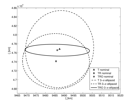
Figure 1: Nominal 2029 $b$-plane coordinates and 3-$\sigma$ uncertainty ellipses for different sets of observations: T is for only Tholen et al. observations, TR is for Tholen et al. plus radar observations, and TRO is for Tholen et al., radar, plus Pan-STARRS PS1 and Magdalena Ridge observations. Note that the axes do not use the same scale.

It is worth noting that the T and TRO nominal solutions are significantly shifted with respect to the TR prediction: the distances in $\sigma$-space are 1.85 and 1.46, respectively. This difference may point to the need for a better data treatment that consists in correcting observations for catalog and proper motion biases, as discussed in Sec. 2.2. It is also interesting to note that the solution obtained with the full dataset is at 0.60 $\sigma$ from the TRO prediction and the improvement in the orbital uncertainty is about 20%. As Królikowska et al. (2009) show that an appropriate selection of the astrometric weighting scheme may be essential for impact predictions, we prefer to use TRO as nominal solution, as we have observations with a more reliable internal consistency and uncertainty estimate.

3 The Yarkovsky effect

The Yarkovsky effect is a nongravitational perturbation that causes asteroids to undergo a secular variation in semimajor axis, resulting in a quadratic in time runoff in anomaly.

As described in Farnocchia et al. (2013), we modeled the Yarkovsky effect as a purely transverse acceleration $a_{t}=A_{2}/r^{2}$, where $r$ is the heliocentric distance and $A_{2}$ is a function of the asteroid’s physical quantities. The corresponding semimajor axis drift can be computed as

$$\frac{da}{dt}=\frac{2A_{2}(1-e^{2})}{np^{2}}\ ,$$ (6)

where $e$ is the eccentricity, $n$ is the mean motion, and $p$ is the semilatus rectum.

As mentioned, $A_{2}$ can be neither computed from the available physical characterization nor estimated from the orbital fit. In fact, with current astrometry we get an uncertainty $\sigma_{A_{2}}=70\times 10^{-15}$ au/d² while the likely range of $A_{2}$ for an object of this size is $\pm 25\times 10^{-15}$ au/d². Therefore, to compute the distribution of the semimajor axis we performed a Monte Carlo simulation as was previously suggested by Chesley et al. (2009). Assumed physical parameters for the simulation were obtained as follows:

• Recent observations from ESA’s Herschel space observatory give a diameter $D=(325\pm 15)$ m (T. Mueller, personal communication). Thus, we used a normal distribution with mean 325 m and standard deviation 15 m (see top left panel of Fig. 2). Herschel observations also provide a geometric albedo $p_{V}=0.23\pm 0.02$. By assuming a slope parameter $G=0.15\pm 0.05$, we converted $p_{V}$ to the Bond albedo $A=(0.29+0.684G)p_{V}$ (Bowell et al., 1989). The top right panel of Fig. 2 shows the distribution of $A$.

• Binzel et al. (2009) report a grain density between 3.4 and 3.6 g/cm³ and a total porosity between 4% and 62%. This leads to a density $\rho$ between 1.29 and 3.46 g/cm³. Therefore, we assumed a lognormal distribution with mean 2.20 g/cm³ and variance 0.3 g²/cm⁶ (see middle left panel of Fig. 2). This distribution is consistent with the constraints of Binzel et al. (2009), as the probability of being smaller than 1.14 g/cm³ or larger than 3.24 g/cm³ is 2.03% and 2.47%, respectively.

• For Apophis the thermal inertia has not yet been measured. Delbò et al. (2007b) find a generic relationship between the thermal inertia and the diameter, according to which $\Gamma=d_{0}D^{-\psi}$, with $d_{0}=(300\pm 45)$ J m^-2 s^-0.5 K^-1, $D$ is in km, and $\psi=0.36\pm 0.09$. Accordingly, we used normal distributions for $\Gamma$ and $\psi$, and combined them with the already available diameter distribution. The middle right panel of Fig. 2 shows the distribution of the thermal inertia.

• Behrend’s asteroids and comets rotation curves website reports a rotation period $P_{rot}=(30.4008\pm 0.0144)$ h, therefore we used the corresponding normal distribution (bottom left panel of Fig. 2).

• The obliquity of the Apophis rotational pole is unknown. Assuming a uniform distribution for the obliquity is a poor approximation. In fact, according to La Spina et al. (2004) retrograde and direct rotators are in a 2:1 ratio within the NEO population. As shown in the bottom right panel of Fig. 2, we used the obliquity distribution from Farnocchia et al. (2013), where the obliquity is inferred from a list of detections of the Yarkovsky effect.

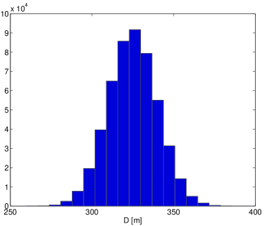
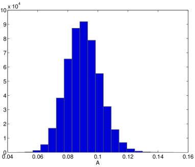
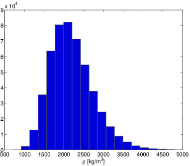
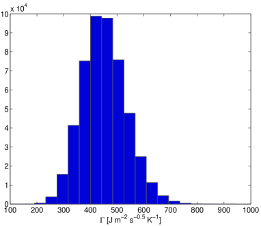
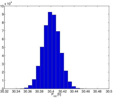
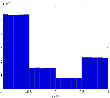
Figure 2: Sampling of Apophis diameter $D$, Bond albedo $A$, density $\rho$, thermal inertia $\Gamma$, rotation period $P_{rot}$, and obliquity $\gamma$.

For each point in the Monte Carlo sampling we computed the associated $A_{2}$ according to Farnocchia et al. (2013), which is based on the linear model of Vokrouhlický et al. (2000), and the orbital drift was then obtained by (6). Figure 3 shows the distribution of $A_{2}$ and $da/dt$. The bimodality of the distributions corresponds to the extreme obliquity peaks.

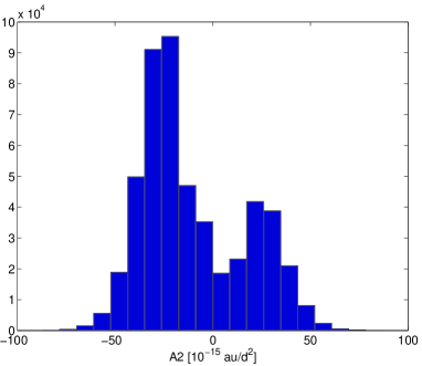
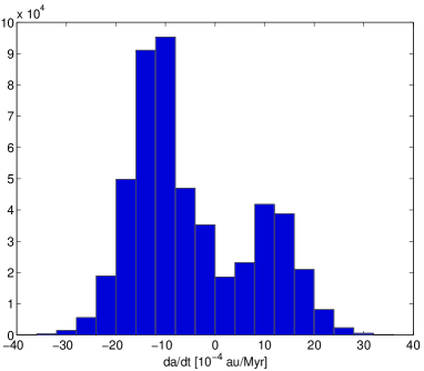
Figure 3: Distribution of $A_{2}$ and $da/dt$ obtained from the assumed physical modeling.

As previously done for the orbital solution uncertainty, we want to see how the Yarkovsky effect maps to the 2029 $b$-plane. To do so we assumed an arbitrary reference value $(A_{2})_{ref}=10\times 10^{-15}$ au/d², corresponding to $(da/dt)_{ref}=4.59\times 10^{-4}$ au/Myr, for which we obtained $\Delta\zeta_{ref}=138.18$ km and $\Delta\xi_{ref}=0.45$ km. This confirms that the Yarkovsky perturbation essentially affects only the $\zeta$ coordinate, which is strongly related to the time and then to the anomaly (Valsecchi et al., 2003). To compute the value of $\Delta\zeta$ for a generic point of the Monte Carlo sampling we scaled from the reference value, after testing the validity of the linear approximation.

4 Keyholes and risk assessment

Even though the 2029 close approach does not lead to an impact, we can use the corresponding $b$-plane analysis to predict future impacts. Valsecchi et al. (2003) show that the $b$-plane coordinates leading to a resonant impact lie on predictable circles. Figure 4 shows the Valsecchi circle on the 2029 $b$-plane for the 2036 resonant return, corresponding to a 7:6 resonance. The Line of Variation (LOV, Milani et al., 2005b) is representative of the orbital uncertainty region. The intersection between the orbital uncertainty region and a Valsecchi circle is a keyhole (Chodas, 1999), leading to a future impact.

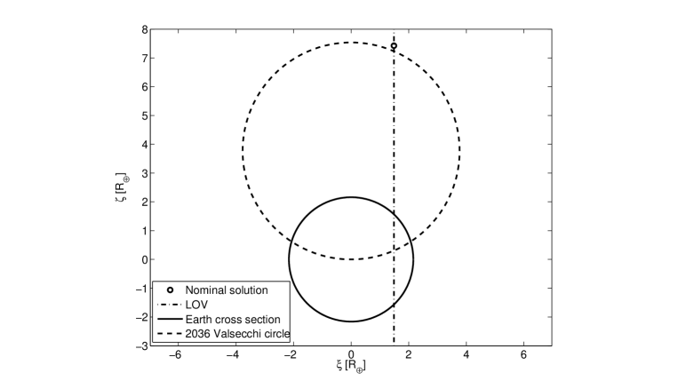
Figure 4: 2036 resonant return, LOV, and keyhole on the 2029 $b$-plane. The impact cross section of the Earth is 2.16 $R_{\oplus}$.

To find the keyholes on the 2029 $b$-plane we propagated a densely sampled LOV through the year 2113, recording the circumstances of all close approaches to Earth and in particular the $b$-plane coordinates, i.e., $(\xi,\zeta)$. On the $b$-plane of a given post-2029 encounter we can interpolate among nearby samples to identify the minimum possible encounter distance along the LOV. When this minimum distance was smaller than 1 Earth radius ($R_{\oplus}$), we obtained the keyhole width by mapping back to the 2029 $b$-plane the chord corresponding to the intersection between the LOV and the Earth cross section. This technique allows us to identify keyholes in 2029 as small as a few centimeters in extent (Table 4). If we plot the minimum encounter distance for each LOV sample over the 100 year integration (and each interpolated local minimum in the encounter distance) against the associated 2029 $b$-plane coordinate $\zeta_{2029}$, then we obtain the plot shown in Fig. 5. The upper panel shows the wider view, which has been extended to the left from nominal to capture the complex of secondary potential impacts surrounding the 2036 primary resonant return that is situated at about $-1500$ km on the abscissa. There are other similar collections of potential impactors in the plot, but the 2036 case is the only one in the depicted $\zeta$ range where the primary return can lead to impact. As an example, the lower panel in Fig. 5 provides a detailed view of the complex of potential impactors situated around $-220$ km on the plot. Here the central post-2029 return, which spawns the surrounding secondary returns, is in 2051, but no impact is possible in that year, although an approach closer than $2R_{\oplus}$ is possible.

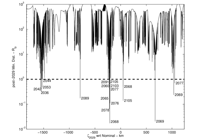
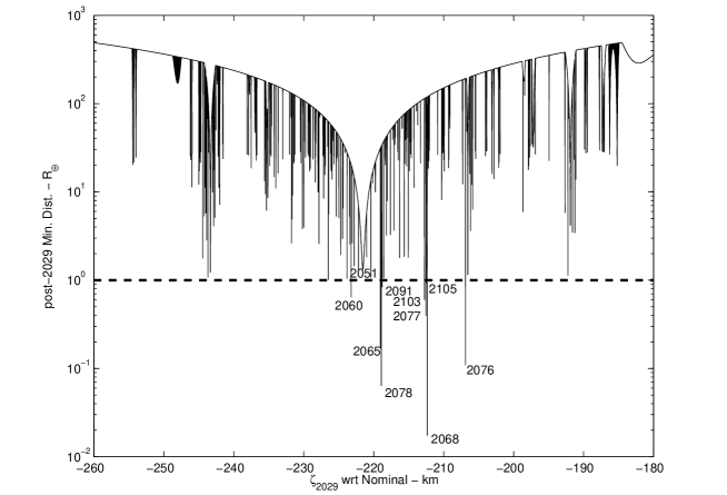
Figure 5: Keyhole map on 2029 $b$-plane. The minimum distance after 2029 is plotted as a function of $\zeta_{2029}$. The top panel shows the full uncertainty region (60000 samples), while the bottom panel is a zoom on the 2051 impactor complex (200000 samples).

Figure 6 shows the $\zeta$ distribution on the 2029 $b$-plane by combining 1) the orbital uncertainty obtained from the orbital fit to the observations neglecting the Yarkovsky effect, and 2) the dispersion due to the Yarkovsky effect. The overall $\zeta$ distribution is therefore obtained as the convolution of the starting probability density functions. It is interesting to see how the overall probability density function (PDF) is close to the Yarkovsky PDF. This is due to the low dispersion of $\zeta$ related to the orbital uncertainty PDF: if the latter were a Dirac delta function, the overall PDF would coincide with the Yarkovsky PDF. The figure also contains the keyholes, where the height of the corresponding bars is determined by the keyhole width. The impact probability can be computed as the product of the width of the keyholes and the PDF. Table 4 reports the information on the keyholes along with the associated impact probability.

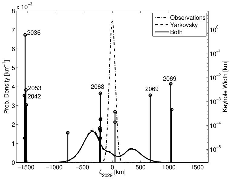
Figure 6: Probability distribution on the 2029 $b$-plane due to the uncertainty in the orbital solution, the Yarkovsky effect, and both. The origin is set to the nominal $\zeta_{2029}=47659.24$ km. Vertical bars correspond to keyholes and the height (in logarithmic scale) is proportional to the keyhole width. For clarity, only the keyholes with a width larger than 1 m are labeled with the year of impact.

Date	width	$\Delta\zeta$ wrt TRO	$\sigma$	IP
TDB	m	km
2042 Apr. 13.5	1.80	-1557.3	-4.80	$1.60\times 10^{-11}$
2041 Apr. 15.3	0.03	-1549.4	-4.78	$3.04\times 10^{-13}$
2036 Apr. 13.4	616.16	-1543.8	-4.77	$7.07\times 10^{-9}$
2053 Apr. 12.9	3.09	-1528.9	-4.73	$4.91\times 10^{-11}$
2044 Apr. 13.3	0.74	-1523.1	-4.71	$1.34\times 10^{-11}$
2089 Oct. 15.6	0.05	-788.7	-2.38	$4.74\times 10^{-9}$
2060 Apr. 12.6	0.03	-223.0	0.08	$3.23\times 10^{-8}$
2065 Apr. 11.8	0.08	-218.8	0.10	$8.40\times 10^{-8}$
2078 Apr. 13.8	0.07	-218.7	0.10	$7.34\times 10^{-8}$
2091 Apr. 13.4	0.07	-218.6	0.10	$7.34\times 10^{-8}$
2103 Apr. 14.4	0.18	-212.5	0.12	$\mathbf{1.82\times 10^{-7}}$
2077 Apr. 13.5	0.06	-212.3	0.12	$6.05\times 10^{-8}$
2105 Apr. 13.8	0.03	-212.3	0.12	$3.03\times 10^{-8}$
2068 Apr. 12.6	2.25	-212.1	0.12	$\mathbf{2.27\times 10^{-6}}$
2076 Apr. 13.0	0.19	-206.7	0.13	$\mathbf{1.85\times 10^{-7}}$
2068 Oct. 15.4	0.14	47.7	0.54	$5.06\times 10^{-8}$
2105 Oct. 16.3	0.38	47.7	0.54	$\mathbf{1.37\times 10^{-7}}$
2069 Oct. 16.0	1.87	671.6	2.24	$\mathbf{2.39\times 10^{-7}}$
2069 Apr. 13.1	5.58	1034.5	3.53	$1.39\times 10^{-8}$
2077 Apr. 13.6	0.47	1052.4	3.59	$9.51\times 10^{-10}$

Table 4: Risk assessment for Apophis. Columns are impact epoch, 2029 keyhole width and location, inverse of the normal cumulative density function, and impact probability. Bold lines correspond to an impact probability larger than Sentry’s generic completeness, i.e., a value of $8.6\times 10^{-8}$ (Milani et al., 2005a).

The results contained in Table 4 depend on the assumptions made on the physical modeling. For example, using a distribution for which a retrograde rotator is so much more likely than a direct one could be inaccurate. In general, we expect that the impact probabilities associated with keyholes close to the peaks of the PDF should be more stable, while those associated with keyholes in the tails of the distribution should be more sensitive to changes in the assumptions because of the exponential decay. To confirm this idea, Table 5 reports the values of the impact probability of the 2036 and 2068 ($\Delta\zeta=-212.14$ km) keyholes, for different assumptions on Apophis’ physical characterization. We can see that the order of magnitude of IP₂₀₆₈ does not change, while IP₂₀₃₆ changes up to three orders of magnitude.

Assumption	2036 IP	2036 $\Delta$IP	2068 IP	2068 $\Delta$IP
Nominal	$7.07\times 10^{-9}$	0%	$2.27\times 10^{-6}$	0%
Diameter $270\pm 60$ m	$3.06\times 10^{-6}$	+43169%	$1.68\times 10^{-6}$	-26%
Unif. $\cos\gamma$	$2.67\times 10^{-9}$	$-62\%$	$2.14\times 10^{-6}$	$-6$%
Symm. $\cos\gamma$	$1.64\times 10^{-9}$	$-77$%	$1.06\times 10^{-6}$	$-53$%
$\sigma_{\rho}^{2}$ = 0.6	$6.60\times 10^{-7}$	$+9242$%	$2.38\times 10^{-6}$	$+5$%
$\mu_{d_{0}}$ = 200	$1.58\times 10^{-9}$	$-78$%	$3.20\times 10^{-6}$	$+41$%
$\mu_{d_{0}}$ = 400	$1.59\times 10^{-8}$	$+125$%	$2.02\times 10^{-6}$	$-11$%

Table 5: Variation of the impact probability for the 2036 and 2068 ($\Delta\zeta=-212.14$ km) keyholes for different assumption the Yarkovsky effect modeling: nominal assumptions of Sec.3; diameter from Delbò et al. (2007a); uniform distribution for $\cos\gamma$; distribution for $\cos\gamma$ symmetric to the one of Fig. 2; different variance of $\rho$; different means of $d_{0}$ in the thermal inertia modeling.

The exceptionally close approach of 2029 may change Apophis’ spin orientation. Scheeres et al. (2005) show that Apophis could exit the 2029 encounter in complex rotation. Therefore, the post-2029 dynamics is a function of $\zeta_{2029}$ and post-2029 $A_{2}$, which we denote with $A^{\prime}_{2}$. In particular, the 2029 keyholes should be considered a two-dimensional entity in $(\zeta_{2029},A^{\prime}_{2})$. Then, the IP of a given keyhole is

$$IP=\int_{-\infty}^{+\infty}\left(f_{1}(\zeta_{2029})w\right)f_{2}(A^{\prime}_{2})dA^{\prime}_{2}$$ (7)

where $f_{1}$ and $f_{2}$ are the PDF of $\zeta_{2029}$ and $A^{\prime}_{2}$, and $w$ is the keyhole width. We checked that for different values of $A^{\prime}_{2}$ the keyhole location changes only slightly (up to 0.5 km) and the width does not change significantly. Therefore, IP does not depend significantly on $A^{\prime}_{2}$.

5 Early 2013 apparition

As already mentioned, the observational dataset available for Apophis does not allow us to measure the Yarkovsky effect from the orbital fit. Apophis is scheduled to be observed from the Goldstone radar observatory in January 2013 and the Arecibo radar observatory in February 2013. Therefore, we wondered whether or not this radar apparition will constrain the Yarkovsky effect. To answer this question we considered three different scenarios:

1. no Yarkovsky effect, i.e., $A_{2}=0$ au/d²;

2. positive orbital drift with $A_{2}=25\times 10^{-15}$ au/d², which corresponds to the right peak of the $da/dt$ distribution of Fig. 3;

3. negative orbital drift with $A_{2}=-25\times 10^{-15}$ au/d², which corresponds to the left peak of the $da/dt$ distribution of Fig. 3.

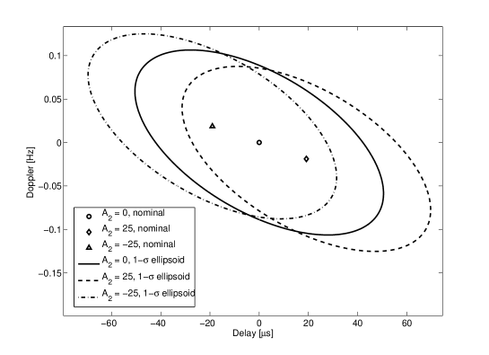
Figure 7: Arecibo delay-Doppler predictions for 2013-02-06.0 for different Yarkovsky scenarios. The origin is set to (127.073088 s, -56954.4 Hz).

Figure 7 shows the predicted values of delay and Doppler measurements for 2013 February 6, for the different scenarios of the Yarkovsky effect. The uncertainty ellipses overlap each other and their intersection contains all the nominal predictions. We conclude that the Yarkovsky effect will not be detectable with the next radar apparition. To further quantify this, we simulated synthetic delay measurements on 2013 February 5 and 6 (see Table 6). As the relative accuracy of delay measurements is $\sim$100 times better than the relative accuracy of Doppler measurements, two delay measurements provide a stronger orbital constraint than a single delay/Doppler pair. For each scenario we tried to determine $A_{2}$ as was done in Farnocchia et al. (2013). We found $\sigma_{A_{2}}=48\times 10^{-15}$ au/d² with the simulated radar data, which is about two times larger than a reasonable value of $|A_{2}|$.

This result may look surprising, since in the cases of (6489) Golevka (Chesley et al., 2003) and 1999 RQ₃₆ (Chesley et al., 2012) the availability of three radar apparitions allowed strong detections of the Yarkovsky effect. However, in these cases the time span covered by radar observations was 12 yr (1991 to 2003 for Golevka, 1999 to 2011 for 1999 RQ₃₆) while for Apophis it is 8 yr. Moreover, the second radar apparitions of Golevka in 1995 and 1999 RQ₃₆ in 2005 were approximately in the middle of the other two, while the second apparition of Apophis was in 2006, just one year after the first apparition, and contains only one Doppler measurement, which is not as precise as delay measurements. Therefore, both the timing and precision of the data may explain the failure in detecting the Yarkovsky effect with three radar apparitions. As a matter of fact, the 2005, 2006, and 2013 datasets essentially contain the same information as two radar apparitions, since only 2005 and 2013 contain delay measurements.

Scenario	$A_{2}$	Date	Delay
	$10^{-15}$ au/d2	UTC	s
(a)	0	2013-02-05.0	124.886779(1)
(a)	0	2013-02-06.0	127.073088(1)
(b)	25.0	2013-02-05.0	124.886797(1)
(b)	25.0	2013-02-06.0	127.073107(1)
(c)	-25.0	2013-02-05.0	124.886760(1)
(c)	-25.0	2013-02-06.0	127.073069(1)

Table 6: Simulated February 2013 delay observations from Arecibo for different values of $A_{2}$. The uncertainty is assumed to be 1 $\mu$s.

At this point it is interesting to see what would be the effect of the January/February 2013 radar apparition on the risk assessment. As the Yarkovsky effect will not be directly detected, the main contribution will be on the orbital uncertainty information. For example, let us consider scenario (c), i.e., we used the radar observations simulated according to the assumed $A_{2}=-25\times 10^{-15}$ au/d². We computed the corresponding orbital solution without accounting for the Yarkovsky effect, which is not measurable. The corresponding 2029 $b$-plane coordinates are $(\xi,\zeta)=(9485.10,47369.09)$ km, with uncertainties 5.30 km and 11.00 km, respectively. While the uncertainty in $\xi$ is almost the same, the uncertainty in $\zeta$ decreased by a factor of 4 and then the corresponding PDF of $\zeta$ due to the orbital uncertainty is even closer to a Dirac delta function. As a consequence, the Yarkovsky PDF and the overall PDF have almost the same curve. The changes in the IP are mostly due to a shift of about -300 km of the nominal Yarkovsky-free prediction. All the virtual impactors (Milani et al., 2005a) of Table 4 persist, and four of them now have an IP$>8.6\times 10^{-8}$: IP${}_{2036}=2.23\times 10^{-7}$, IP${}_{2068}(\Delta\zeta=-212.14km)=6.95\times 10^{-7}$, IP${}_{2068}(\Delta\zeta=47.68km)=1.03\times 10^{-7}$, and IP${}_{2105}=2.79\times 10^{-7}$.

Though the Yarkovsky effect will not be constrained, radar and optical photometry can provide independent information to improve Apophis’ physical modeling. In particular, it may be possible to further constrain the diameter and the albedo, and to estimate the spin orientation, which would allow us to remove the bimodality in the Yarkovsky distribution.

The next opportunity for radar observations is the September 2021 close approach. Meanwhile, ground based optical observations are possible and can help in determining the Yarkovsky effect before the September 2021 close approach. Table 7 contains the uncertainty in the $A_{2}$ determination by assuming simulated radar observations in February 2013 and progressively adding simulated ground based optical observations weighted at 0.15”. We conclude that the Yarkovsky effect would be significantly constrained between late 2020 and early 2021.

Dates	$\sigma_{A_{2}}$ [$10^{-15}$ au/d2]
Jan. 2013 – Jun. 2013	47
Sep. 2013 – May 2015	40
Oct. 2015 – Jan. 2016	39
Mar. 2018 – May 2018	32
Dec. 2018 – Aug. 2020	16
Nov. 2020 – May 2021	4

Table 7: Uncertainty in the Yarkovsky effect determination as a function of increasing number of simulated optical observations weighted at 0.15”. For each interval we simulated one observation every two months.

6 Conclusions

In this paper we presented an updated and careful impact risk analysis for asteroid (99942) Apophis. The presence of the scattering close approach in 2029 calls for accurate orbit estimation and dynamical modeling. Therefore, we selected astrometry for which the uncertainty information is rigorously computed by the observer and added the contributions of observatories with comparable performance. To model the Yarkovsky effect we performed a Monte Carlo simulation relying on the best physical model currently available.

We obtained the distribution on the 2029 $b$-plane by combining the orbital uncertainty and the dispersion due to the Yarkovsky effect. We then found twenty keyholes corresponding to future impacts and computed the corresponding impact probabilities. In particular, we found a $2.27\times 10^{-6}$ impact probability for an impact in 2068.

We analyzed the stability of the computed impact probabilities with respect to the assumed Apophis’ physical characterization. Impacts corresponding to keyholes close to the nominal solution have a stable impact probability (the order of magnitude does not change). On the other hand, for keyholes in the tails of the distribution we found variations up to three orders of magnitude.

We also showed that the February 2013 radar apparition will not allow a direct detection of the Yarkovsky effect, and therefore the post-2029 possibility of impact will not be ruled out. The main contribution will be a reduction of the orbital uncertainty, thus making the dispersion due to the Yarkovsky the predominant source of uncertainty.

References

- Baer et al. (2011) Baer, J., Chesley, S. R., Matson, R. D., 2011. Astrometric Masses of 26 Asteroids and Observations on Asteroid Porosity. The Astronomical Journal 141, 143.
- Bancelin et al. (2012) Bancelin, D., Colas, F., Thuillot, W., Hestroffer, D., Assafin, M., 2012. Asteroid (99942) Apophis: new predictions of Earth encounters for this potentially hazardous asteroid. Astronomy and Astrophysics 544, A15.
- Binzel et al. (2009) Binzel, R. P., Rivkin, A. S., Thomas, C. A., Vernazza, P., Burbine, T. H., DeMeo, F. E., Bus, S. J., Tokunaga, A. T., Birlan, M., 2009. Spectral properties and composition of potentially hazardous Asteroid (99942) Apophis. Icarus 200, 480–485.
- Bottke et al. (2006) Bottke, W. F., Vokrouhlický, D., Rubincam, D. P., Nesvorný, D., 2006. The Yarkovsky and YORP Effects: Implications for Asteroid Dynamics. Annual Review of Earth and Planetary Sciences 34, 157–191.
- Bowell et al. (1989) Bowell, E., Hapke, B., Domingue, D., Lumme, K., Peltoniemi, J., Harris, A. W., 1989. Application of photometric models to asteroids. In: Binzel, R. P., Gehrels, T., Matthews, M. S. (Eds.), Asteroids II. pp. 524–556.
- Carry (2012) Carry, B., 2012. Density of asteroids. Planetary and Space Science 73, 98–118.
- Chesley (2006) Chesley, S. R., 2006. Potential impact detection for Near-Earth asteroids: the case of 99942 Apophis (2004 MN4). In: Lazzaro, D., Ferraz-Mello, S., Fernández, J. A. (Eds.), Asteroids, Comets, Meteors. Vol. 229 of IAU Symposium. pp. 215–228.
- Chesley et al. (2010) Chesley, S. R., Baer, J., Monet, D. G., 2010. Treatment of star catalog biases in asteroid astrometric observations. Icarus 210, 158–181.
- Chesley et al. (2009) Chesley, S. R., Milani, A., Tholen, D., Bernardi, F., Chodas, P., Micheli, M., 2009. An Updated Assessment Of The Impact Threat From 99942 Apophis. In: AAS/Division for Planetary Sciences Meeting Abstracts #41. Vol. 41 of AAS/Division for Planetary Sciences Meeting Abstracts. p. #43.06.
- Chesley et al. (2012) Chesley, S. R., Nolan, M. C., Farnocchia, D., Milani, A., Emery, J., Vokrouhlický, D., Lauretta, D. S., Taylor, P. A., Benner, L. A. M., Giorgini, J. D., Brozovic, M., Busch, M. W., Margot, J.-L., Howell, E. S., Naidu, S. P., Valsecchi, G. B., Bernardi, F., 2012. The Trajectory Dynamics of Near-Earth Asteroid 101955 (1999 RQ36). LPI Contributions 1667, 6470.
- Chesley et al. (2003) Chesley, S. R., Ostro, S. J., Vokrouhlický, D., Čapek, D., Giorgini, J. D., Nolan, M. C., Margot, J.-L., Hine, A. A., Benner, L. A. M., Chamberlin, A. B., 2003. Direct Detection of the Yarkovsky Effect by Radar Ranging to Asteroid 6489 Golevka. Science 302, 1739–1742.
- Chodas (1999) Chodas, P. W., 1999. Orbit uncertainties, keyholes, and collision probabilities. Bulletin of the Astronomical Society 31, 2804.
- Delbò et al. (2007a) Delbò, M., Cellino, A., Tedesco, E. F., 2007a. Albedo and size determination of potentially hazardous asteroids: (99942) Apophis. Icarus 188, 266–269.
- Delbò et al. (2007b) Delbò, M., Dell’Oro, A., Harris, A. W., Mottola, S., Mueller, M., 2007b. Thermal inertia of near-Earth asteroids and implications for the magnitude of the Yarkovsky effect. Icarus 190, 236–249.
- Farnocchia et al. (2013) Farnocchia, D., Chesley, S. R., Vokrouhlicky, D., Milani, A., Spoto, F., Bottke, W. F., 2013. Near Earth Asteroids with measurable Yarkovsky effect. Icarus (In press).
- Folkner (2011) Folkner, M. K., 2011. Planetary ephemeris DE424 for Mars Science Laboratory early cruise navigation. JPL IOM 343R-11-003.
- Gilmore et al. (2004) Gilmore, A. C., Kilmartin, P. M., Young, J., McGaha, J. E., Garradd, G. J., Beshore, E. C., Casey, C. M., Christensen, E. J., Hill, R. E., Larson, S. M., McNaught, R. H., Smalley, K. E., 2004. 2004 MN4. Minor Planet Electronic Circulars Y, 25.
- Giorgini et al. (2008) Giorgini, J. D., Benner, L. A. M., Ostro, S. J., Nolan, M. C., Busch, M. W., 2008. Predicting the Earth encounters of (99942) Apophis. Icarus 193, 1–19.
- Gleason et al. (2004) Gleason, A. E., Larsen, J. A., Descour, A. S., Williams, G. V., 2004. 2004 MN4. MPEC Y, 70.
- Konopliv et al. (2011) Konopliv, A. S., Asmar, S. W., Folkner, W. M., Karatekin, Ö., Nunes, D. C., Smrekar, S. E., Yoder, C. F., Zuber, M. T., 2011. Mars high resolution gravity fields from MRO, Mars seasonal gravity, and other dynamical parameters. Icarus 211, 401–428.
- Królikowska et al. (2009) Królikowska, M., Sitarski, G., Sołtan, A. M., 2009. How selection and weighting of astrometric observations influence the impact probability. The case of asteroid (99942) Apophis. Monthly Notices of the Royal Astronomical Society 399, 1964–1976.
- La Spina et al. (2004) La Spina, A., Paolicchi, P., Kryszczyńska, A., Pravec, P., 2004. Retrograde spins of near-Earth asteroids from the Yarkovsky effect. Nature 428, 400–401.
- Milani et al. (2009) Milani, A., Chesley, S. R., Sansaturio, M. E., Bernardi, F., Valsecchi, G. B., Arratia, O., 2009. Long term impact risk for (101955) 1999 RQ36. Icarus 203, 460–471.
- Milani et al. (2005a) Milani, A., Chesley, S. R., Sansaturio, M. E., Tommei, G., Valsecchi, G. B., 2005a. Nonlinear impact monitoring: line of variation searches for impactors. Icarus 173, 362–384.
- Milani et al. (2012) Milani, A., Knežević, Z., Farnocchia, D., Bernardi, F., Jedicke, R., Denneau, L., Wainscoat, R. J., Burgett, W., Grav, T., Kaiser, N., Magnier, E., Price, P. A., 2012. Identification of known objects in Solar System surveys. Icarus 220, 114–123.
- Milani et al. (2005b) Milani, A., Sansaturio, M. E., Tommei, G., Arratia, O., Chesley, S. R., 2005b. Multiple solutions for asteroid orbits: Computational procedure and applications. Astronomy and Astrophysics 431, 729–746.
- Monet et al. (2003) Monet, D. G., Levine, S. E., Canzian, B., Ables, H. D., Bird, A. R., Dahn, C. C., Guetter, H. H., Harris, H. C., Henden, A. A., Leggett, S. K., Levison, H. F., Luginbuhl, C. B., Martini, J., Monet, A. K. B., Munn, J. A., Pier, J. R., Rhodes, A. R., Riepe, B., Sell, S., Stone, R. C., Vrba, F. J., Walker, R. L., Westerhout, G., Brucato, R. J., Reid, I. N., Schoening, W., Hartley, M., Read, M. A., Tritton, S. B., 2003. The USNO-B Catalog. The Astronomical Journal 125, 984–993.
- Moyer (2003) Moyer, T. D., 2003. Formulation for Observed and Computed Values of Deep Space Network Data Types for Navigation. Wiley-Interscience, Hoboken, NJ.
- Russell et al. (2012) Russell, C. T., Raymond, C. A., Coradini, A., McSween, H. Y., Zuber, M. T., Nathues, A., De Sanctis, M. C., Jaumann, R., Konopliv, A. S., Preusker, F., Asmar, S. W., Park, R. S., Gaskell, R., Keller, H. U., Mottola, S., Roatsch, T., Scully, J. E. C., Smith, D. E., Tricarico, P., Toplis, M. J., Christensen, U. R., Feldman, W. C., Lawrence, D. J., McCoy, T. J., Prettyman, T. H., Reedy, R. C., Sykes, M. E., Titus, T. N., 2012. Dawn at Vesta: Testing the Protoplanetary Paradigm. Science 336, 684–686.
- Scheeres et al. (2005) Scheeres, D. J., Benner, L. A. M., Ostro, S. J., Rossi, A., Marzari, F., Washabaugh, P., 2005. Abrupt alteration of Asteroid 2004 MN4’s spin state during its 2029 Earth flyby. Icarus 178, 281–283.
- Skrutskie et al. (2006) Skrutskie, M. F., Cutri, R. M., Stiening, R., Weinberg, M. D., Schneider, S., Carpenter, J. M., Beichman, C., Capps, R., Chester, T., Elias, J., Huchra, J., Liebert, J., Lonsdale, C., Monet, D. G., Price, S., Seitzer, P., Jarrett, T., Kirkpatrick, J. D., Gizis, J. E., Howard, E., Evans, T., Fowler, J., Fullmer, L., Hurt, R., Light, R., Kopan, E. L., Marsh, K. A., McCallon, H. L., Tam, R., Van Dyk, S., Wheelock, S., 2006. The Two Micron All Sky Survey (2MASS). The Astronomical Journal 131, 1163–1183.
- Tholen et al. (2012) Tholen, D. J., Micheli, M., Elliott, G. T., 2012. Improved Astrometry of (99942) Apophis. Acta Astronautica (In press).
- Tholen et al. (2013) Tholen, D. J., Micheli, M., Elliott, G. T., 2013. The Effect of Proper Motion on Pan-STARRS Asteroid Astrometry. Icarus (In press).
- Žižka and Vokrouhlický (2011) Žižka, J., Vokrouhlický, D., 2011. Solar radiation pressure on (99942) Apophis. Icarus 211, 511–518.
- Valsecchi et al. (2003) Valsecchi, G. B., Milani, A., Gronchi, G. F., Chesley, S. R., 2003. Resonant returns to close approaches: Analytical theory. Astronomy and Astrophysics 408, 1179–1196.
- Vokrouhlický et al. (2000) Vokrouhlický, D., Milani, A., Chesley, S. R., 2000. Yarkovsky Effect on Small Near-Earth Asteroids: Mathematical Formulation and Examples. Icarus 148, 118–138.
- Zacharias et al. (2003) Zacharias, N., McCallon, H. L., Kopan, E., Cutri, R. M., 2003. Extending the ICRF Into the Infrared: 2MASS-UCAC Astrometry. In: Gaume, R. A., McCarthy, D. D., Souchay, J. (Eds.), IAU Joint Discussion. Vol. 16 of IAU Joint Discussion. pp. 52–59.