Parallel Algorithms for Constructing Data Structures for Fast Multipole Methods

Abstract

We present efficient algorithms to build data structures and the lists needed for fast multipole methods. The algorithms are capable of being efficiently implemented on both serial, data parallel GPU and on distributed architectures. With these algorithms it is possible to map the FMM efficiently on to the GPU or distributed heterogeneous CPU-GPU systems. Further, in dynamic problems, as the distribution of the particles change, the reduced cost of building the data structures improves performance. Using these algorithms, we demonstrate example high fidelity simulations with large problem sizes by using FMM on both single and multiple heterogeneous computing facilities equipped with multi-core CPU and many-core GPUs.

1 Introduction

$N$-body problems evaluate the weighted sum of a kernel function $\Phi(\mathbf{y},\mathbf{x}_{i})$ centered at $N$ source locations $\{\mathbf{x}_{i}\}$ for all $M$ receiver locations $\{\mathbf{y}_{j}\}$ with the strengths $q_{i}$ (Eq. 1). They can also be viewed as dense $M\times N$ matrix vector products. Direct evaluation of this method on CPU has the quadratic $O(NM)$ complexity. Such direct evaluations cannot be scaled to large sizes required by high fidelity simulations.

$$\phi(\mathbf{y}_{j})=\displaystyle\sum_{i=1}^{N}q_{i}\Phi(\mathbf{y}_{j}-\mathbf{x}_{i}),\ \ j=1,2,\ldots,M,\ \ \mathbf{x}_{i},\mathbf{y}_{j}\in\mathbb{R}^{d},$$ (1)

Hardware acceleration, such as [1] using the GPU and [2] using specially constructed hardware called the “Gravity Pipe”(GRAPE), can only speedup the sum to some extent but do not address its quadratic complexity.

An alternative way to evaluate such sums for particular kernels is to use fast approximation algorithms, for example, the Fast Multipole Method [3], the Barnes-Hut Method [4] and the Particle-Mesh Methods [5], which have lower asymptotic complexity when they are applicable. Since the FMM can achieve linear complexity but achieve guaranteed accuracy up to machine precision, we only focus on this method in this paper, however the data structure techniques used here may find application in the other fast algorithms also, and indeed wherever computations involve particles.

The FMM exactly computes near-field interactions but approximates far-field interactions to a specified tolerance $\epsilon$. It splits the summation in Eq. 1 into near and far fields as

$$\phi(\mathbf{y}_{j})=\displaystyle\sum_{\mathbf{x}_{i}\in\Omega(\mathbf{y}_{j})}q_{i}\Phi(\mathbf{y}_{j}-\mathbf{x}_{i})+\sum_{\mathbf{x}_{i}\not\in\Omega(\mathbf{y}_{j})}q_{i}\Phi(\mathbf{y}_{j}-\mathbf{x}_{i})$$ (2)

for $j=1,2,\ldots,M$ where $\Omega$ is the neighborhood domain. The first term on the right hand side of Eq. 2 can be computed exactly at $O(N)$ cost given a fixed cluster size, i.e., the maximal number of data points inside any neighborhood domain. To approximate the second term, the kernel function is factored into an infinite sum, which is truncated at $p$ terms according to the required accuracy, by using singular (multipole) spherical basis functions, $S_{l}$, and regular (local) spherical basis functions $R_{l}$. These factorizations can be used to separate the kernel computations involving the points sets either $\{\mathbf{x}_{i}\}$ or $\{\mathbf{y}_{j}\}$, and consolidate operations for many points as

$$\begin{array}[]{l}\displaystyle\sum_{\mathbf{x}_{i}\not\in\Omega(\mathbf{y}_{j})}q_{i}\Phi(\mathbf{y}_{j}-\mathbf{x}_{i})=\displaystyle\sum_{\mathbf{x}_{i}\not\in\Omega(\mathbf{y}_{j})}q_{i}\sum_{l=0}^{p-1}S_{l}(\mathbf{y}_{j}-\mathbf{x}_{\ast})R_{l}(\mathbf{x}_{i}-\mathbf{x}_{\ast})\\ =\displaystyle\sum_{l=0}^{p-1}S_{l}(\mathbf{y}_{j}-\mathbf{x}_{\ast})\sum_{\mathbf{x}_{i}\not\in\Omega(\mathbf{y}_{j})}q_{i}R_{l}(\mathbf{x}_{i}-\mathbf{x}_{\ast})=\displaystyle\sum_{l=0}^{p-1}C_{l}S_{l}(\mathbf{y}_{j}-\mathbf{x}_{\ast}),\end{array}$$ (3)

The $p$ coefficients $C_{l}$ for all $\mathbf{x}_{i}$ are built in $pN$ operations and then they can be used in the evaluation at all $\mathbf{y}_{j}$ in $pM$ operations. This approach reduces the cost of evaluating the far-field contributions as well as the memory requirement to $O(N+M)$.

Because the factorization in Eq. 3 is not global, the split between the near- and far-fields must be managed, which requires appropriate data structures and the use of a variety of representations for the function. The efficiency with which the data structures are constructed is very important for dynamic problems since the source and receiver points change their positions at every time step. We propose novel parallel algorithms for the data structures for both single and multiple heterogeneous nodes.

1.1 Well-separated Pair Decomposition

The need to construct spatial data structures arise from a need to provide an error controlled translation of the FMM function representations (discussed below in Section 1.4). This is achieved using a well-separated pair decomposition (WSPD), which is itself useful for solving a number of other geometric problems [6, chapter 2]. In the context of FMM, given the distance between the two sphere centers $d$, with radii are $r_{A}$ and $r_{B}$ respectively, the translation error $\varepsilon$ (from $c_{A}$ to $c_{B}$) is bounded by

$$\varepsilon(p)<C\eta^{p}{(r_{A},r_{B})},\quad\eta(r_{A},r_{B})=\frac{\max(r_{A},r_{B})}{d-\min(r_{A},r_{B})}$$ (4)

where $p$ is the truncation number. Note that the $p$ is determined based on the worst case. In the FMM data structures, this WSPD is realized by the octree spatial decomposition (Refer to theoretical results from [7]).

1.2 The Baseline FMM Algorithm

The FMM was first introduced by Greengard and Rokhlin in [3] and has been identified as one of the ten most important algorithmic contributions of the 20th century [8].

The multi-level FMM (MLFMM) puts sources into hierarchical space boxes and translates the consolidated interactions of sources into receivers. For the convenience of presentation, we call a box containing at least one source point a source box and a box containing at least one receiver point a receiver box. The FMM algorithm can be summarized as four main parts: the initial expansion, the upward pass, the downward pass and the final summation.

1. Initial expansion (P2M):

   1. In the finest level $l_{max}$, all the source data points are expanded at their box centers to obtain the far-field $\mathcal{M}$ expansion coefficients $\{\mathcal{C}_{n}^{m}\}$ over $p^{2}$ spherical basis functions.

   2. The obtained $\mathcal{M}$-expansion from all source points within the same boxes are consolidated into a single expansion at each box center.

2. Upward pass (M2M): For levels from $l_{max}$ to 2, the $\mathcal{M}$ expansion coefficients for each box are evaluated via the multipole-to-multipole ($\mathcal{M}|\mathcal{M}$) translations from the source boxes to their parent source box. All these translations are performed in a hierarchical order from bottom to top via the octree.

3. Downward pass: For levels from 2 to $l_{max}$, each receiver box also generates its local or $\mathcal{L}$ expansion in a hierarchical order from top to bottom via the octree.

   1. M2L: Translate multipole $\mathcal{M}$ expansion coefficients from the source boxes of the same level belonging to the receiver box’s parent neighborhood but not the neighborhood of that receiver itself, to local $\mathcal{L}$ expansion via multipole-to-local ($\mathcal{M}|\mathcal{L}$) translations then consolidate the expansion coefficients.

   2. L2L: Translate the $\mathcal{L}$ expansion coefficients (if the level is 2, then these expansions are set to be 0) from the parent receiver box center to its child box centers and consolidate with the same level multipole-to-local translated expansions.

4. Final summation (L2P: Evaluate the $\mathcal{L}$ expansion coefficients for all the receiver points at the finest level $l_{max}$ and performs a local direct sum of nearby source points within their neighborhood domains.

Note that the local direct sum is independent of the far-field expansions and translations, thus may be scheduled on different computing hardware concurrently for high performance efficiency. Moreover, it is important to balance costs between these pairwise kernel sums and the hierarchical translations to achieve high computation throughput and proper scaling. Besides those algorithmic considerations, there is another vital factor to achieve such desired high efficiency: low data addressing latency. In our implementation, both translations and local direct sums have their special auxiliary interaction lists used to address data directly. Therefore, the FMM algorithm requires the following special data structures:

1. octree to ensure WSPD that ensures error bounds.

2. interaction lists for fast data addressing.

3. the communication management structures.

The construction of these data structures must be done via algorithms that have the same overall complexity with the summation.

1.3 Treecode and Its Data Structures

Similar to the FMM, there is also another well-known fast $N$-body simulation algorithm, Barnes-Hut-Method [4], which uses the similar spatial data structures as FMM and is often called a treecode. As in the FMM, the whole space is hierarchically subdivided via an octree. Each spatial box has an pseudo-particle that contains the total mass in the box located at the center of mass of all the particles it contains. Whenever force on a particle is required, the tree is traversed from the root. If a certain box is far away from that particle, the pseudo-particle is used to approximate the force induced by that box, otherwise it is subdivided again or is processed particle–by–particle directly. The complexity of treecode is in $O(N)$. However, unlike FMM, the control on the accuracy is less precise.

In the most recent GPU treecode development [9], algorithms for the octree traversing, particle sorting and data compaction (skip empty boxes) on GPU based on the cuda scan algorithm [10]. Such algorithms, are similar to the approaches in Section 2.1 and which we first presented in [11]. The other work in the treecode space that is similar, is [12], in which a GPU-based construction of space filling curves (SFC) and octrees were presented.

1.4 Multi-Level FMM Data Structures

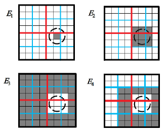
Figure 1: $E_{1},E_{2},E_{3},E_{4}$ neighborhoods of dimension 2: red division at level 1; blue division at level 2; black division at level 3. The shaded box in $E_{1}$ sub-figure has its Morton index as 40 at level 2.

Assume all of the data points are already scaled into a unit cube. The WSPD is recursively performed by subdividing the cube into subcubes (spatial boxes) via an octree until the maximal level, $l_{max}$, or the tree depth, is achieved (The level $l_{max}$ is chosen such that the computational costs of the local direct sums and the far-field translations can be balanced to the extent possible). To guarantee separation of spatial data points by these subcubes and their minimal bounding spheres, we need to introduce several different space neighborhood domains [13]. Given each spatial cubic box with the Morton index [6, 14] $n=0,\ldots,2^{ld}$ at level $l=0,\ldots,l_{max}$ in $d$ dimensions,

1. $E_{1}(n,l)\subset\mathbb{R}^{d}$ denotes the spatial points inside the box $n$ at level $l$. We call these boxes as source or receiver box with index $n$ at level $l$.

2. $E_{2}(n,l)\subset\mathbb{R}^{d}$ denotes the spatial points in the neighborhood of the box with index $n$ at level $l$ (“neighborhood” means all its immediate neighbor boxes). This list is used for local direct summations for $E_{1}(n,l)$.

3. $E_{3}(n,l)=\overline{E_{2}(n,l)}\subset\mathbb{R}^{d}$ denotes spatial points outside the neighborhood of the box $n$ at level $l$. This is the complement of $E_{2}(n,l)$.

4. $E_{4}(n,l)=E_{2}($ParentIndex$(n),l-1)\backslash E_{2}(n,l)\subset\mathbb{R}^{d}$ denotes spatial points inside the neighborhood of the parent box ParentIndex($n$) at level $l-1$ but which do not belong to the neighborhood of box $n$ at level $l$. These are interaction boxes whose contributions are accounted for by M2L translations for $E_{1}(n,l)$.

Consider any box $B$ with Morton index $n$ at level $l$ (see Fig. 1). All the translation operations are performed box by box so the source data have to be viewed as spatial boxes but not individual points. All the receiver data points inside $B$ can not be well separated with all the source boxes inside $E_{2}(n,l)$. Hence $E_{2}(n,l)$ is used to compute the near-field sum. Due to hierarchical translations, all the source boxes outside $E_{4}(n,l)$ have already been translated to $B$’s center at the previous level. Thus only the influence of the remaining source data needs to be translated. These are located in its $E_{4}(n,l)$ domain, which corresponds to the most time consuming $M|L$ translation to $B$.

In [15] and [13], they described those FMM related octree data structures and their implementations in details. Similar work on such hierarchical spatial data structures can be found [16] and [17].

In the literature, the data structure research mainly focuses on load balancing and data partition. In [18], several opportunities for parallelism in the FMM were discussed and it was shown that it is possible to apply FMM on both shared memory or distributed architectures. Compared to later work, the data distribution method in this pioneering paper was simple, perhaps not practical in many applications. In [19], an efficient parallel adaptive FMM with a “costzones” partition technique was developed based on data locality. A multi-threaded tree construction was implemented in [20]. However, in these papers the data structures were not built in parallel, i.e, the local tree of each node was built by a single processor. In [21] and [22] they separated the computation and communication to avoid synchronization during the evaluation passes. Ref. [23] extended the work of [21] by providing a new parallel tree construction and a novel communication scheme, which scaled up to billion size problem on 65K cores. But all the GPUs were only used for kernel evaluation, i.e. direct local sum and part of translations, while the data structures alone were sequentially constructed within a single node on CPUs. In contrast, our approach provides parallel algorithms to build data structures not only on the node level, but also at a much finer granularity within a node, which allows their construction algorithms to be efficiently mapped on SIMD architectures of GPUs. There are also many other works focusing on a complementary problem: of partitioning the FMM data across multiple processors, such as [24], which shown a provably and efficient good partition as well as a load balancing algorithm, and [25], which presented a partition strategy based on precomputated parameters.

1.5 Parallel Hardware

There is a revolution underway over the past decade or so in the use of graphics inspired hardware for accelerating general purpose computation. Since GPUs are attached to the host (CPU) via PCI-Express bus, processing data on those accelerators requires data transfer between host and device (GPU). The on-chip memory are hierarchical and the programming focus is to best use these hierarchical memories in the threaded model efficiently given the trade-off between speed and size [26, 27].

On the many-core GPU accelerators, the data are processed as warps, i.e, a group of threads executing the same instruction at the same time and thousands of threads are spawned to run in parallel. Hence, the parallel algorithms presented in this paper are designed for performance efficiency under this architecture which favors massively parallel threads and accounts for the cost of memory access. In this paper, we only focus on the parallel programming presentations under the NVIDIA GPUs and CUDA, nevertheless our algorithms could be implemented similarly by using OpenCL [26, 28] or on different many-core accelerators being introduced such as the AMD APU/GPU or INTEL XEON PHI.

1.6 Motivation for Fast Data Structure Algorithms

Several papers in the literature as we mentioned before ([9, 12], etc.) have been published on fast Kd-tree and octree data structures that look similar to the spatial data structures used here, however, they lack the functionality to construct these interaction lists for the specific neighbor and box query operations, hence cannot be directly applied in to the FMM framework. The typical way of computing these data structures is via an $O(N\log N)$ algorithm, which is built upon spatial data sorting and is sequentially implemented on the CPU [29]. For large dynamic problems (the particle positions change every time step), this data structure construction cost would dominate the overall cost by Amdahl’s law, especially when the FMM kernel evaluation is significantly speeded up. Reimplementing the CPU algorithm for the GPU would not achieve the kind of acceleration we sought. The reason is that the conventional FMM data structures algorithm employs sorting of large data and operations such as set-intersection and searching, that require random access to the global memory, cannot be implemented efficiently on current GPU architectures.

2 Single Node Parallel FMM Data Structure Algorithm

The basic FMM data structures in our implementations are based on the octree [6, chapter 2]. At different octree levels, the unit cube containing all the spatial points is hierarchically divided into sub-cubes via an octree and each spatial box is assigned a global Morton index [14]. Basic concepts and operations on the octree data structures include: finding neighbor boxes, assigning indices and finding coordinates of the box center via interleaving/deinterleaving, particle location (box index) query, etc. Refer to [15, 13] for details of these basic concepts, operations and algorithms.

The algorithm is based on use of occupancy histograms (i.e., the counts of particles in each box), assigning particles to their grid cells, and parallel scans [30]. A disadvantage of this approach is the fact that the histogram requires temporary allocation of an array of size $8^{l_{\max}}$. Nonetheless this algorithm for GPUs with 4 GB global memory enables of data structures up to a maximum level $l_{\max}=8$, which is sufficient for many problems. In this case accelerations up to two orders of magnitude compared to CPU were achieved. Note that the histogram is only needed at the time of data structure construction, all the empty box information is skipped in the final data structure outputs, which are passed to the real FMM kernel evaluation engine, to achieve both high memory and subsequent summation efficiency.

We would first like to establish some notation. First of all, all the integers in our implementation, such as box indices, histograms, are stored as unsigned int. We use Src/Recv to represent source points/receiver points respectively. We define non-empty source/receiver boxes as those boxes that contain at least one source/receiver data point respectively, while empty source/receiver boxes have no points inside. Note that an empty source box may contain receiver points and vice versa.

2.1 Pseudo-Sort Using Fixed-Grid-Method in Linear Time

To build the FMM data structures, we first need to reorganize the data points (both source and receiver) into a tree structure according to their spatial locations, such that at the finest level each octree box holds at most a prescribed number of points, the cluster size. By adjusting the cluster size, we can try to ensure that the costs of the near-field direct sums and the far-field approximated sums are roughly balanced (or take the same time). Given the cluster size, we could determine the maximal level $l_{max}$ of the octree. The data reorganization is realized by a “Fixed-Grid-Method” algorithm, in which all data points are rearranged according to their Morton box indices at level $l_{max}$ but only with linear computation cost, since the order of data points within a box, which share the same Morton index, is irrelevant to the algorithm correctness. We don’t use the word “sort” here is because this pseudo-sort is a nondeterministic algorithm. In our GPU implementation, the final sort order is determined by the run-time global memory access order of CUDA threads.

Since we have to pseudo-sort both source and receiver points, we use the term “data points” to refer to both, and denote the array storing these data points by P[]. Firstly, each data point P[i] has associated with a 2D vector called sortIdx[i], where sortIdx[i].x stores the Morton index of its box and sortIdx[i].y stores its rank within the box. Secondly, there is a histogram array Bin[] allocated for the boxes at the maximal level. Its $i$th entry Bin[i] stores the number of data points within the box $i$, which is computed by the atomicAdd() function in the GPU implementation. This CUDA function performs a read-modify-write atomic operation on one 32-bit or 64-bit word residing in global or shared memory [27]. Let the number of data points be $M$. Then the pseudocode to compute sortIdx[] and Bin[] is given in Alg. 1.

Algorithm 1 Parallel-Pseudo-Sort(P[], M): an algorithm to compute the sorted index of each particle using the Fixed-Grid-Method.

1:a particle position array P[] with length M

2:a 2D index array sortIdx[]

3:for i=0 to M-1 parallel do

4:     SortIdx[i].x$\leftarrow$BoxIndex(P[i])

5:     atomicAdd[Bin[SortIdx[i].x]]

6:     SortIdx[i].y$\leftarrow$Bin[SortIdx[i].x]

Although atomicAdd() serializes those threads that access the same memory address, the parallel performance of our implementation is good on average. This is because most threads work on different memory locations at the same time. After this pseudo-sort, all the data points are copied into a new sorted array according to their sortIdx and their corresponding bookmark arrays (a pointer array described in details in Sec. 2.2), which is used to find the data points given a box Morton index, are constructed. Note that the cost to move data and write the pointer address into the bookmarks are also linear and moving data on the device can take advantage of high GPU memory bandwidth. We denote the pseudo-sorted source/receiver point arrays as SortedSrc[]/SortedRecv[] respectively.

2.2 Interaction Lists

To access data efficiently, we use several pre-computed arrays, which are also constructed by using parallel algorithms on the GPU: SrcBookmark[], RecvBookmark[], NeighborList[], SrcNonEmptyBoxIndex[], and NeighborBookmark[]. We call these interaction lists. Define $\mathtt{numSrcNEBox}$ and $\mathtt{numRecvNEBox}$ be the number of non empty source and receiver boxes respectively. We describe these interaction lists below:

• SrcBookmark[]: its $i$th entry points to the first sorted source data point in the $i$th source non-empty box in SortedSrc[] Its length is $\mathtt{numSrcNEBox+1}$.

• RecvBookmark[]: its $j$th entry points to the first sorted receiver data point in the $j$th receiver non-empty box in SortedRecv[]. Its length is $\mathtt{numRecvNEBox+1}$.

• SrcNonEmptyBoxIndex[]: its $i$th entry stores the Morton index of the $i$th non-empty source box. Its length is $\mathtt{numSrcNEBox}$.

• NeighborBookmark[]: to perform the local direct sum of the $j$th non-empty receiver box, its $E_{2}$ neighbor information can be retrieved from the NeighborBookmark[j]$th$ to the NeighborBookmark[j+1]-1$th$ enties in the list NeighborList[].

• NeighborList[]: given two indices $i$ and $j$ such that NeighborBookmark[j] $\leq i<$ NeighborBookm- ark[j+1] and denote $k=i-$NeighborBookmark[j], then NeighborList[i] stores the index of the $k$th non-empty source box adjacent to the $j$th non-empty receiver box ($E_{2}$ neighborhood). Here the index means the rank of that non-empty source box in the SrcNonEmpty- BoxIndex[]. See figure 2.

• RecvPermutationIdx[]: its $i$th entry means the original position of data point SortedRecv[i] in Recv[] is Rec- vPermutationIdx[i].

Algorithm 2 Access-Source-$E_{2}$-neighborhood( SortedSrc[], SrcBookmark[], NeighborList[], NeighborBookmark[], i): an algorithm to extract all the source data within the $E_{2}$ neighborhood of the $i$th (non-empty) receiver box.

1:the $i$th receiver box and other interaction lists

2:the source data tempSrcNei[] within its $E_{2}$ neighborhood

3:count$\leftarrow$0

4:tempSrcNei$\leftarrow\emptyset$

5:B$\leftarrow$NeighborBookmark[i+1]-1

6:for j=NeighborBookmark[i] to B do

7:     v$\leftarrow$NeighborList[j];

8:     C$\leftarrow$SrcBookmark[v+1]-1

9:     for k=SrcBookmark[v] to C do

10:         tempSrcNei[count++]$\leftarrow$SortedSrc[k]      

Given the bookmark array, the data point can be accessed directly from the sorted data list. For each receiver non-empty box, the source data points within its $E_{2}$ neighborhood can be accessed as Alg. 2. The bookmarks are only kept for non-empty boxes and the neighbor list is only kept for non-empty neighbors. No information of empty boxes are passed to the FMM kernel evaluation engine. The last auxiliary array RecvPermutationIdx[] is used to retrieve the input order of the original receiver data points.

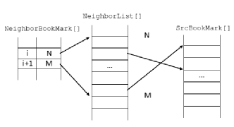
Figure 2: The mapping relation among the neighbor bookmark, the neighbor list and the source bookmark

2.3 Parallel Data Structure Construction

Algorithm 3 Get-bookmark-and-box-index(Bin[]): an algorithm to compute the bookmark and the non-empty box index of source/receiver boxes.

1:the pseudo-sorted index array Bin[] of source/receiver boxes

2:the bookmark array Bookmark[] and the Morton index array NonEmptyIdx[] of source/receiver boxes $\triangleright$ array indices depend on implementations

3:perform parallel scan on Bin[] to obtain its prefix sum ScannedBin[]

4:for i=0 to Bin[].length-1 parallel do

5:     if Bin[i]>0 then

6:         Rank[i]$\leftarrow$1

7:     else

8:         Rank[i]$\leftarrow$0      

9:perform parallel scan on Rank[] to obtain its prefix sum ScannedRank[]

10:allocate memory for Bookmark[] and NonEmptyIdx[] $\triangleright$ their lengths can be derived from Bin[]

11:Bookmark[0]$\leftarrow$0

12:Bin[-1]$\leftarrow$0

13:for i=0 to Bin[].length-1 parallel do

14:     if Bin[i]>Bin[i-1] then

15:         Bookmark[ScannedRank[i]]$\leftarrow$Bin[i]

16:         NonEmptyIdx[ScannedRank[i]]$\leftarrow$i      

Algorithm 4 Get-$E_{2}$-neighbor-list-and-bookmark( Scanned- Rank[], RecvNonEmptyBoxIdx[], numNonEmptyRecvBox): an algorithm to extract the $E_{2}$ neighborhood for all the (non-empty) receiver boxes.

1:the ScannedRank[] from Alg. 3 for source, the receiver box index array RecvNonEmptyBoxIdx[] with its length numNonEmptyRecvBox

2:The $E_{2}$ neighbor list array NeighborList[] (for receiver boxes) and its bookmark NeighborBookmark[]

3:allocate a temporary array RecvE2NeiNEBoxIdx[] to store neighbor box indices $\triangleright$ each box can have 27 neighbors at most in 3D

4:for i=0 to numNonEmptyRecvBox-1 parallel do

5:     $n_{i}\leftarrow$0

6:     k$\leftarrow$RecvNonEmptyBoxIdx[i]

7:     for all its non-empty $E_{2}$ source neighbor box $j$ do

8:         NeighborIdx[27i+($n_{i}$++)]$\leftarrow j$      

9:     NumRecvE2NeiNEBox[i]$\leftarrow n_{i}$

10:     for j=0 to $n_{i}-1$ do

11:         RecvE2NeiNEBoxIdx[27i+j]=ScannedRank[Nei- ghborIdx[j]-1]      

12:perform parallel scan on NumRecvE2NeiNEBox[] to obtain its prefix sum NeighborBookmark[]

13:allocate NeighborList[] $\triangleright$ itself and its length can be derived from RecvE2NeiNEBoxIdx[] and NeighborBookmark[] respectively

14:for i=0 to numNonEmptyRecvBox-1 parallel do

15:     for j=0 to NumRecvE2NeiNEBox[i]-1 do

16:         count $\leftarrow$ NeighborBookmark[i]+j

17:         NeighborList[count]$\leftarrow$RecvE2NeiNEBoxIdx[27i+j]      

In our implementation, the bookmark for the source/receiver box is the rank of its first source/receiver point among all source/receiver points. The bookmark provides a pointer to the data of any non-empty box among all boxes without search. A reduction operation is needed to compute the entries of the bookmark arrays. The highly efficient parallel prefix sum (or scan) [10] is used in our implementation. Given the Bin[] obtained from Alg. 1, the Bookmark[] can be computed by removing the repeated elements (corresponding to empty boxes) in the prefix sum of Bin[] using Alg. 3. The same idea can also be used to address any non-empty source/receiver box among all source/receiver boxes if we mark non-empty boxes by 1 and empty boxes by 0 and apply the scan operation. With Bookmark[] and SortIdx[], data points are copied to into a new sorted list. SrcNonEmptyBoxIndex[] is used to construct NeighborBookmark[] and NeighborList[] in parallel as Alg. 4: initially a thread computes the $E_{2}$ neighbor box indices of a non-empty receiver box and checks whether these source neighbor boxes are empty or not. Then this thread increases the local non-empty source box count accordingly for its assigned receiver box and store the neighbor indices temporarily. Finally after another parallel scan call, the temporary neighbor indices are compressed and written to NeighborList[], where the target address is obtained by reading the non-empty source box index from SrcNonEmptyBoxIndex[]. Algorithm 5 summarizes all the steps to build the data structures for a single computing node.

Algorithm 5 Build-fmm-data-structures(Src[], Recv[]): the single-node algorithm to pseudo-sort data points and construct all the needed interaction lists on GPU.

1:the source/receiver data Src[]/Recv[]

2:all interaction lists and the pseudo-sorted source/receiver data SortedSrc[]/SortedRecv[]

3:pseudo-sort Src[] by Alg. 1

4:get SrcNonEmptyBoxIndex[] and SrcBookmark[] by Alg. 3

5:copy sorted source data points to SortedSrc[]

6:pseudo-sort Recv[] by Alg. 1

7:get RecvPermutationIdx[] and RecvBookmark[] by Alg. 3

8:copy sorted receiver data points to SortedRecv[];

9:build NeighborBookmark[] and NeighborList[] by Alg. 2 and Alg. 4

10:pass SortedSrc[], SrcBookmark[], SortedRecv[], RecvBookmark[], RecvPermutationIdx[], Neighbor- Bookmark[] and NeighborList[] to FMM kernel evaluation engine;

11:free all other allocated device memory;

All the octree operations needed in Alg. 5, can be found in [15]. By using the interleave and deinterleave operations, we can derive a 3D coordinate for any given Morton index. Given this 3D vector, we can increase or decrease its coordinate component to compute its neighbors’ 3D coordinates. Therefore, the algorithms of $E_{2}$ and $E_{4}$ neighbor queries can be easily obtained. Accordingly, they are not presented as separate algorithms. Note that, given any spatial box, the computations of its neighbors’ coordinates and Morton indices are independent of other boxes and executed in parallel.

2.4 GPU Implementation Considerations

Basic octree operations, such as box index query, box center query, box index interleave/deinterleave and parent/children query, and more complex neighbor query operations, such as $E_{2}$ and $E_{4}$ neighbor index query, are all implemented as inlined CUDA __device__ functions. For efficiency, we minimize the use of global memory and local memory accessing. Once input data is loaded into these device functions, we only use local fast registers, or coalesced local memory if data can not fit into registers, to store intermediate results. Moreover, we manually unroll many loops to further optimize the code. Results shows that even for the costly computation of $E_{4}$ neighbors, its total running time can be neglected in comparison with the kernel evaluation time in the FMM.

2.5 Complexity

The complexity of these data structure algorithms is determined by the number of source points $N$, the number of receiver points $M$ and the maximal octree level $l_{max}$. Since we use histograms, we can avoid all the searching operations on the device, which makes our implementation fast and efficient. However, there is a memory consumption trade-off for the processing speed since the size of histogram increases exponentially as $l_{max}$. For the bucket sort Alg. 1, its complexity is linear $O(N+M)$. All other algorithms are related to the octree boxes, which total number is $N_{box}=2^{3l}=8^{l}$. Since we use the canonical scan algorithm, Alg. 2 to Alg. 4 are in $O(N_{box}\log N_{box}+N+M)\sim O(l8^{l}+N+M)$. If we interpret the maximal level $l_{max}$ as a prescribed constant, then our parallel data structure construction Alg. 5 for single node is linear with respect to particle size, i.e. in $O(N+M)$.

3 FMM Data Structures on Multiple Nodes

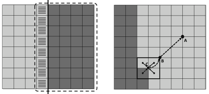
Figure 3: Problems in distributing the FMM across two nodes. Left: lightly-shaded boxes are on node 1 (Partition I) and darkly shaded boxes are on node 2 (Partition II). The thick line indicates the partition boundary line and the dash line shows the source points in both partitions needed by Partition II. The hashed boxes are in Partition I but they have also to be included in Partition II to compute the local direct sum. Right: light boxes belong to Partition I and dark boxes belong to Partition II. The multipole coefficients of the box with thick lines (center at C) is incomplete due to one child box on another node. Hence its parents (B and A) in the tree up to the minimal level are all incomplete.

Since all the data structures are constructed based on the locations of source and receiver data points, there are two main issues on the multiple nodes. First, on multiple nodes using the algorithm of [31, 32], only receiver data points are mutual exclusively distributed. Source points which are in the halo regions (boundary layers of partitions) have to be distributed on several nodes, because of the direct sum region overlap. Hence on each node, the source data points for direct sum and translation are no longer the same. When we build the translation data structure, these repeated source data should be guaranteed to translate only once among all the nodes. Second, since any translation stencils may require coefficients from many source boxes which are on other nodes, there will be many translation coefficient communications among different nodes. Moreover, due to the partition, from a certain level on, the octree box coefficients on a single node might be incomplete up to the root of the octree. This is because if one of any box’s children is distributed on one or several different nodes, all its ancestors coefficients are incomplete. In Fig. 3, we show such an example. Finally, all information related to these boxes are stored in a compressed way because we skip all empty boxes. Therefore it is a non-trivial task to fetch the coefficients of any box efficiently since many searching and rearranging data operations are needed. Good partition and data communication algorithms are crucial to reduce the communication overhead in terms of both data transfer size and data packing time.

3.1 Global Data Structure and Partitioning

In [31] FMM algorithms for the heterogeneous CPU-GPU architecture were explored and it was concluded that a good strategy is to distribute the FMM computation components between CPUs and GPUs: expensive but highly parallizable particle related computations (direct sums) are assigned to the GPU, while the extensive and complex space box related computations (translations) are assigned to CPU. This way one can take the best advantages of both CPU and GPU hardware architecture, and we design our data structures for this mapping.

The split of the global octree can be viewed as a forest of $K$ trees with roots at level 2 and leaves at level $l_{max}$. In the case of more or less uniform data distributions and number of nodes less than $K\leq 64$ (for the octree), each node may handle one or several trees. If the number of nodes are more than 64 and/or data distributions are substantially non-uniform, partitioning based on the work load balance can be performed by splitting the trees at levels $>$ 2. Such partitioning can be thought as breaking of some edges of the initial graph. This increases the number of the trees in the forest, and each tree may have a root at an arbitrary level $l=2,...,l_{max}$. Each node then takes care for computations related to one or several trees. At this point we assume that there exists some work load balancing algorithm which provides an efficient partitioning. At this point we also do not put any constraint to interaction between the receiver and source trees, so formally this can be considered as two independent partitions.

For presentation purposes, we define two important concepts although they are related to each other in our implementation:

• partition level $l_{par}$: at this level, the whole space are partitioned among different computing nodes. On a local node, all the subtrees at this level or below are totally complete, i.e., no box at level $\geq l_{par}$ is on other nodes.

• critical level $l_{crit}$: at this level, all the box coefficients are broadcasted such that all boxes at level $\leq l_{crit}$ can be treated as local boxes, i.e., all the box coefficients are complete after broadcasting. In our implementation, $l_{crit}=\max{(l_{par}-1,2)}$.

Normally the number of computing nodes in current high performance clusters are in the order of hundreds or even thousands, that is considered much smaller than the number of spatial boxes of the global octree. Hence, the partition level is usually quite low, such as $l_{par}=2,3,4$. Hence broadcasting the coefficients at the critical level $l_{crit}$ only requires a small amount of data with neglectable communication overhead given the major cost of kernel evaluations.

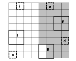
Figure 4: An example of source box types. White boxes are Partition I and gray boxes are Partition II. The partition level is 3 and the critical level is 2. Solid line boxes correspond to level 2 and dash line boxes correspond to level 3. At partition II, box $\mathbf{e}$ and $\mathbf{E}$ are export boxes. Boxe $\mathbf{i}$ and $\mathbf{I}$ are import boxes. Box $\mathbf{R}$ is a root box. Box $\mathbf{d}$ is a domestic box. Box $\mathbf{o}$ is an other box.

To better organize data communication, on each node, we classify all the source boxes into five categories in an array SrcNonEmptyBoxType[]. From the finest level $l_{max}$ to 2, we list all the global source box Morton indices in an increasing order. Note that some local empty source boxes might be in the list since this box may contain source points which are located on other nodes and this global source boxes information is obtained from the initial global octree construction. Given those box types, we could determine which boxes need to import or export their $M$-coefficients. For any node, say $J$, these five box types are (see Fig. 4):

1. Domestic Boxes: The box and all its children are on $J$. All domestic boxes are organized in trees with roots located at level 1. All domestic boxes are located at levels from $l_{max}$ to 2. The roots of domestic boxes at level 1 are not domestic boxes (no data is computed for such boxes).

2. Export Boxes: These boxes need to send data to other nodes. At $l_{crit}$, the M-data of export boxes may be incomplete. At level $>l_{crit}$, all export boxes are domestic boxes of $J$ and their M-data are complete.

3. Import Boxes: Their data are produced by other computing nodes for importing to $J$. At $l_{crit}$, the M-data of import boxes may be incomplete. At level $>l_{crit}$, all import boxes are domestic boxes of nodes other than $J$ and their M-data are complete there.

4. Root Boxes: These are boxes at critical level, which need to be both exported and imported. For level $>l_{crit}$ there is no root box.

5. Other Boxes: Boxes which are included in the data structure but do not belong to any of the above types, e.g. all boxes of level 1, and any other box, which for some reason is passed to the computing node (such boxes are considered to be empty and are skipped in computation, so that affects only the memory and amount of data transferred between the nodes).

Note that there are no import or export boxes at levels from $l_{crit}-1$ to 2. All boxes at these levels are either domestic boxes or other boxes after the broadcast and summation of incomplete $M$-data at $l_{crit}$. We only need compute M-data and box types from level $l_{max}$ to $l_{crit}$ and exchange the information at $l_{crit}$. After that we compute the $M$-data for all the domestic boxes up to level 2 then produces $L$-data for all receiver boxes at level $l_{max}$ handled by the computing node.

3.2 FMM Algorithm on Multiple Nodes

Our multiple node algorithm involves three main parts:

1. Global source and receiver data partition: the partition should keep work balance among all the computing nodes.

2. Single node evaluation: a single node performs the translations upward/downward, compute the export and import data and the local summations.

3. Multiple node data exchange: The data communication manager collects and distributes the data from/to all the computing nodes accordingly.

Parts (2) and (3) are mutually inclusive because the translations on a single node require the missing data from other nodes while the data communication requires import and export information from each computing node. Part (1) depends on the application. For dynamic problems, the FMM evaluation is performed for every time step and the data distribution can be derived from the previous time step. It is very likely that all the nearby data are stored on the same node, in which case the partition to keep work balance only requires a small amount of communication. For problems only performing a single FMM evaluation, the data appear on each node might be dependent on some geometric properties but it is also possible that the initial data on each node is random, in which case a large amount of the inter-node communications is inevitable. In our implementation, we assume the worst case that all the data on each node are random.

3.2.1 Global Partition

The architecture of our computing system, and perhaps of most current and near future systems, is heterogeneous. Each node has several multicore CPUs and one or two many-core GPUs. While the CPU cores on the same node share the main memory, each GPU has its own dedicated device memory, connected to host via PCI-Express bus. To perform computations on GPUs, the data for a single node have to be divided again for each GPU. As mentioned before, we perform direct sums on GPUs and FMM translation on CPUs, hence we need two level partition: divide the data for nodes first (translation) then further divide data cdof each node for each GPU (direct sum). Given the prescribed cluster size, we construct the global octree then split it, i.e., the partition of all the data is performed by boxes but not by particles.

Assume the same number $g$ of GPUs on each computing node, then we implement this two level partition as follow: we assign a unique global ID $(ig+j)$ to the $j$th GPU on the node $i$ and compute our finer partition with respect to those GPUs. From $l_{par}=2$, our algorithm tries to distribute all the boxes at level $l_{par}$ among GPUs such that the amount of receiver points satisfy the prescribed balance conditions. It increases the $l_{par}$ by 1 until the work load balance is roughly achieved. Once this finer partition is done, we automatically obtain a balanced coarse partition with respect to computing nodes (this is because each node has the same number of GPUs). To identify all box locations, we use an auxiliary array BoxProcId[], in which $i$th entry stores the GPU ID where the $i$th box at $l_{par}$ resides in. Dividing BoxProcId[i] by $g$, we can obtain the node ID where the $i$th box resides in. Note that, for any given box at any level, we can easily answer its location query by shifting that box’s Morton index and examining BoxProcId[], i.e. by checking its ancestor/children’s location. Initially, we use GPUs and Alg. 1 to pre-process data, i.e. to get the number of receiver points in each box. Then all nodes send their Bin[] array to the master node. The master node then computes the balanced partition and derives the value of $l_{par}$ such that each GPU is assigned several spatial boxes at $l_{par}$ with consecutive Morton indices. Finally, the master node broadcasts this partition information to all the nodes and each nodes distributes its own source and receiver data based on the partition to others.

3.2.2 The FMM Algorithm on Multiple Nodes

Assume that the balanced global data partition and distributed data are available. On one hand, the data structure constructions of local neighbor interaction lists for direct sum are the same as section 2. On the other hand, the data structures of translations are for the coarse partition (with respect to node), hence they need to be recomputed by merging the octree data structures obtained from multiple GPUs on the same node. The merging steps are conducted as follows

1. Extract all the global source box information across all the computing nodes: after all GPU calls the data structure construction call of section 2, each node collects these non-empty source box indices from all its GPU, merges to one list and send to the master node. Then the master node merges all the lists to one global non-empty source box array and broadcasts to all nodes.

2. Extract the local receiver box information for each node: each node collects these non-empty receiver box indices from all its GPU, merges to one list. Because each GPU deals with consecutive receiver boxes, this merging is actually equivalent to copy operations.

Once these two box index arrays are available, we can construct the interaction lists for translation stencils, in parallel on GPU. Except the source box type, the algorithm for which will be described later, all other needed information arrays, such as neighbor lists/bookmark etc, can be obtained by using the algorithms in section 2. Each node $J$ then executes the following translation algorithm:

1. Upward translation pass:

   1. Get M-data of all domestic source boxes at $l_{max}$ from GPU global memory.

   2. Produce M-data for all domestic source boxes at levels $l=l_{max}-1,\ldots,\max(2,l_{crit})$.

   3. Pack export M-data, the import and export box indices of all levels. Then send them to the data exchange manager.

   4. The master node, which is also the manager, collects data. For the incomplete root box M-data from different nodes, it sums them together to get the complete M-data. Then according to each node’s export/import box indices, it packs the corresponding M-data then sends to them.

   5. Receive import M-data of all levels from the data exchange manager.

   6. If $l_{crit}>2$, consolidate $S$-data for root domestic boxes at level $l_{crit}$. If $l_{crit}>3$, produce M-data for all domestic source boxes at levels $l=l_{crit}-1,\ldots,2$.

2. Downward translation pass:

   1. Produce L-data for all receiver boxes at levels $l=2,\ldots,l_{max}$.

   2. Output L-data for all receiver boxes at level $l_{max}$.

   3. Redistribute the L-data among its own GPUs.

   4. Each GPU finally consolidates the L-data, add the local sums to the dense sums and copy them back to the host according to the original inputting receiver’s order.

When each node outputs its import box index array, they are listed in an increasing order from $l_{max}$ to $l_{crit}$. The manager processes the requesting import box index array one after another. Given the $i$th requested source box index ImportSrcIdx[i], the manager first figures out its level $l_{*}$. If $l_{*}<l_{crit}$, the manager derives ImportSrcIdx[i]’s ancestor in the partition level and check the array BoxProcId[] to find which node it belongs to. If $l_{*}==l_{crit}$, the manager will check all its children’s node address ($l_{*}$ can not exceed $l_{crit}$ since all the boxes above the critical level are marked as domestic box). Once the manager identifies the node ID, where that box belongs to or its children belong to, it searches the export box index array from that node for ImportSrcIdx[i] at level $l_{*}$ then makes an copy of the corresponding $M$-data in the sending buffer.

Even though each node handles a large number of spatial boxes, the amount information exchanged with the manager is actually small since only boxes on the partition boundary layers need to be transferred back and forth. In our current implementation, the manager is responsible for all the collecting and redistributing $M$-data work, which involves searching operations, the total run time is still smaller by comparing with the communication scheme of [31], where all the box’s $L$-data ($O(p^{2}8^{l})$ in the case of uniform distribution) at the finest level $l_{max}$ are broadcast from the master node.

3.2.3 Source Box Type

The type of a source box $\mathbf{k}$ is determined by the M2M and M2L translation because its children or neighbors might be missing due to data partition and have to be requested from other nodes. However, once the parent box M-data is complete, the L2L translations for its children are always complete. So we can summarize the key idea of Alg. 6, which computes the type of each box, as follows:

• At the critical level, we need all boxes to perform upward M2M translations. If one child is on a node other than $J$, its M-data is either incomplete or missing, hence we mark it an import box. We also check its neighbors required by M2L translation stencil. If any neighbor is not on $J$, then the M-data of these two boxes have to be exchanged.

• For any box at the partition level or deeper levels, if this box is not on $J$, then it is irrelevant to this node, in which case it is marked as other box. Otherwise we check all its neighbors required by M2L translations. Again if any neighbor is not on $J$, these two boxes’ M-data have to be exchanged.

Algorithm 6 Get-source-box-type(BoxIndex[],ParInfo,$J$): the algorithm to compute the source box types on the Node $J$ given the partition information

1:a source box index BoxIndex[i]$=\mathbf{k}$ at level $l$, the partition information and the node ID $J$

2:BoxType[i]

3:isOnNode$\leftarrow$isImportExport$\leftarrow$isExport$\leftarrow$FALSE

4:if $l$<$l_{crit}$ then

5:     BoxType[i]$\leftarrow$DOMESTIC

6:else if $l$=$l_{crit}$ then

7:     for any $\mathbf{k}$’s child $\mathbf{c}_{i}$ at partition level do

8:         if $\mathbf{c}_{i}$ is not on $J$ then

9:              isImportExport$\leftarrow$TRUE

10:         else

11:              isOnNode$\leftarrow$TRUE               

12:     if isOnNode=FALSE then

13:         BoxType[i]$\leftarrow$IMPORT

14:     else

15:         for any $\mathbf{k}$’s neighbor of M2L translation $\mathbf{n}_{i}$ do

16:              if one of $\mathbf{n}_{i}$’s children at $l_{crit}$ is not on $J$ then

17:                  isExport$\leftarrow$TRUE $\triangleright$ update the type of a different box

18:                  $\mathbf{n}_{i}$’s box type $\leftarrow$IMPORT                             

19:else

20:     if  $\mathbf{k}$’s ancestor at $l_{crit}$ is not on $J$ then

21:         BoxType[i]$\leftarrow$OTHERS

22:     else

23:         for any $\mathbf{k}$’s neighbor of M2L translation $\mathbf{n}_{i}$ do

24:              if the ancestor of $\mathbf{n}_{i}$ at $l_{crit}$ is not on $J$ then

25:                  isExport$\leftarrow$TRUE$\triangleright$ update the type of a different box

26:                  $\mathbf{n}_{i}$’s box type $\leftarrow$IMPORT                             

27:synchronize all threads

28:if isImportExport=TRUE then

29:     BoxType[i]$\leftarrow$ROOT

30:else if isExport=TRUE then

31:     BoxType[i]$\leftarrow$EXPORT

32:else

33:     BoxType[i]$\leftarrow$DOMESTIC

We compute all box types in parallel on the GPU. For each level from $l_{max}$ to 2, a group of threads on the node $J$ are spawned and each thread is assigned by one source box index at that level. After calling Alg. 6, all these threads have to be synchronized before the final box type assignment in order to guarantee no race conditions. Note that some “if-then” conditions in Alg. 6 can be replaced by OR operations so that thread “divergent branches” can be reduced.

3.3 Complexity

Lets assume that we have $P$ computing nodes and each node has $g$ GPUs. We only count non-empty boxes here and all symbols are used as follows: $B^{src}_{i,l}$ and $B^{recv}_{i,l}$ are the numbers of local source and receiver boxes at level $l$ on the $i$th node respectively; $B^{src}_{all,l}$ is the number of global source boxes at level $l$; $N_{i}$ and $M_{i}$ are the numbers of source and receiver points on the $i$th node respectively; $N$ and $M$ are the total numbers across all the nodes.

First, we estimate the running time of our global partition given the worst case (the initial data are totally random):

$$T_{1}=a_{0}(N_{i}+M_{i})+a_{1}B^{recv}_{i,l_{max}}+a_{2}B^{recv}_{all,l_{max}}+a_{3}B^{recv}_{all,l_{max}}\log P+a_{4}(N+M).$$ (5)

Each term within the equation (5) is described in table 1. Note that, moving $O(N+M)$ data points is inevitable if the initial data on each node are random, however in many applications, this communication cost can be avoided or reduced substantially if this initial distribution is known. Also there are many publications on this initial partition (tree generation) and optimized communication in the literature such as [24, 21, 25], which can be used for different applications accordingly.

Term	Description
$a_{0}(N_{i}+M_{i})$	each node derives the local box Morton indices for its source and receiver points and sends them
$a_{1}B^{recv}_{i,l_{max}}$	each node sends its receiver box indices at the finest level to the master node
$a_{2}B^{recv}_{all,l_{max}}$	the master node collects all the receiver box indices and builds the global indices
$a_{3}B^{recv}_{all,l_{max}}\log P$	the master node broadcasts the global receiver box indices and partition
$a_{4}(N+M)$	all nodes exchange source and receiver data according to the partition (including a node-wide synchronization)

Table 1: Description of equitation (5)

Second, Alg. 6 examines the occupancy status of each source box’s $E_{4}$ neighbors. Note that the number of $E_{4}$ neighbors for any octree box is upper bounded by 27 and for each neighbor such check operation is in constant time. Hence the cost to compute all source box types can be estimated as:

$$T_{2}=b_{0}B^{src}_{all,l_{max}}+b_{1}B^{src}_{all,l_{max}-1}+\ldots+b_{l_{max}-2}B^{src}_{all,2}\leq b_{*}B^{src}_{all,l_{max}}.$$ (6)

Finally, let’s denote $B^{src}_{all}=\sum_{j=2}^{l_{max}}B^{src}_{all,j}$. There is no clean model to estimate the number of export/import boxes. However, the boundary of each partition is nothing but a surface of some 3D object. Given the uniform distribution case, in which we can simplify the model, it is reasonable to estimate the exchanged box number as $\mu 2^{2l_{max}}=\mu 4^{l_{max}}$ with some constant $\mu$ for all the nodes ([23] estimate this number as $O((B^{recv}_{i,l_{max}})^{2/3})$, which is similar as ours). Therefore, at the critical level $l_{crit}$, the exchanging data cost can be estimated as:

$$T_{3}=c_{0}B^{src}_{all}+c_{1}\mu 4^{l_{max}}p^{2}+c_{2}\mu 4^{l_{max}}\log(\mu 4^{l_{max}})+c_{3}8^{l_{crit}}p^{2}.$$ (7)

Term	Description
$c_{0}B^{src}_{all}$	each node examines its source box types and extracts import and export source box indices
$c_{1}\mu 4^{l_{max}}p^{2}$	each node sends the export box’s $M$-data to the master node
$c_{2}\mu 4^{l_{max}}\log(\mu 4^{l_{max}})$	the master node addresses all the requested import box indices of each node
$c_{3}8^{l_{crit}}p^{2}$	the master node packs all the import $M$-data and sends to other corresponding nodes

Table 2: Description of equitation (7)

Each term in the equation (7) is explained in table 2. By combining some constant coefficients, we can further simplify $T_{3}$ as

$$T_{3}$$ = ,

= .

(8)

Because those three parts are executed sequentially, $T$, the total cost of communications and data structures, can be obtained as

$$\begin{array}[]{rl}T=&T_{1}+T_{2}+T_{3}=T_{gpu}+T_{cpu}+T_{comm},\textrm{ where}\\ T_{gpu}\leq&a_{0}M_{i}+a_{1}B^{recv}_{i,l_{max}}+b_{*}B^{src}_{all,l_{max}}\\ =&a_{0}M/P+a_{1}B^{recv}_{all,l_{max}}/P+b_{*}B^{src}_{all,l_{max}},\\ T_{cpu}=&d_{0}B^{src}_{all}+d_{1}l_{max}4^{l_{max}},\\ T_{comm}=&d_{2}(4^{l_{max}}+d_{3}8^{l_{crit}})p^{2}+a_{2}B^{recv}_{all,l_{max}}+a_{3}B^{recv}_{all,l_{max}}\log P\\ &+a_{4}(N+M).\end{array}$$ (9)

The ideal algorithm should have all costs proportional to $1/P$. In our case, only the particle related terms but not all the box related terms are amortized among all the computing nodes. However, in practical, $l_{max}$ can not be very large which is viewed as a constant in most cases. More sophisticated schemes can be used so that these theoretical non-scalable terms can be amortized among all the nodes. However, given our parallel implementation, the constant coefficient for each term is small even when the box number is large. Hence $T_{gpu}$ and $T_{cpu}$ could be negligible compared with the kernel time.

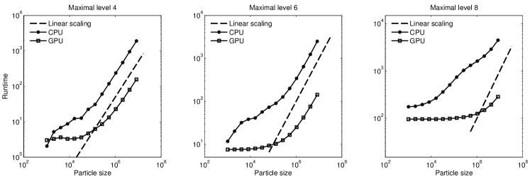
Figure 5: The data structure construction time for non-uniform distribution on a single node using one GPU: all the source and receiver are distributed on a sphere. Each sub-figure corresponds to a maximal level setting.

As for the communication part, the real killing communication comes from $a_{4}(N+M)$ since we target on billion scale problems. Exchanging all these particle data requires much more time than the real kernel evaluations. However, this term is not encountered usually because it is obtained from the worst case, that is the totally random distribution. In most application, based on the physical or geometric properties, this initial data distribution can be configured such that only small amount of particle communication is needed. Moreover, as mentioned before, we could use the parallel partition methods in literature to minimize this cost. All other terms in $T_{comm}$ are still scalable since they are determined by the number of non-empty spatial boxes ($\ll N$ or $M$) and these costs are much less than the kernel evaluation time.

4 Experimental Results

4.1 Single Node Algorithm Test

To test the data structure performance for a single node, we fix the problem size to 1 million and use the uniform distributed source and receiver. Here the source and receiver points are different. The computation hardware used here are: NVIDIA GTX480 GPU and Intel Xeon X5560 quad-core CPU running at 2.8GHz.

$l_{\max}$	CPU (ms)	Improved CPU (ms)	GPU (ms)
3	1293	223	7.7
4	1387	272	13.9
5	2137	431	13.0
6	8973	1808	34.6
7	30652	6789	70.8
8	58773	7783	124.9

Table 3: The time comparison of FMM data structure computation for $2^{20}$ uniform randomly distributed source and receiver particles using our original CPU $O(N\log N)$ algorithm, the improved $O(N)$ algorithm on a single CPU core, and its GPU accelerated version.

We firstly test the performance on the uniformly distributed data in a unit cube. Note that, this would be most time consuming case since almost all the spacial boxes are non-empty. The timing results are summarized in Table 3, in which the octree depth was varied in the range $l_{\max}=3,...,8$. Column 2 shows the wall clock time for a standard algorithm, which uses sorting and hierarchical neighbor search using set intersection (the neighbors were found in the parent neighborhood domain subdivided to the children level). Column 3 shows the wall clock time for the present algorithm on the CPU. It is seen that our algorithm is several times faster. Comparison of the GPU and CPU times for the same algorithm show further acceleration in the range 20-100.

In the second experiment, we generate all the source and receiver data on a sphere surface and test how the algorithm scales and the performance gain. In Figure 5, we show both the CPU and GPU time across the number of data points, which ranges from 1024 up to 8 millions, for different octree maximal levels. As the $l_{max}$ increases, there are more spatial boxes occupied which super linearly increases the overall costs. However, once the number boxes become relative stable, i.e., increasing the number of particles only changes the number of spatial boxes a little bit, the overall cost increases linearly. This is because that all the boxes related constructions is more or less the same as a constant and the particle related computation, such as bit interleaving and the fixed-grid-method pseudo-sort that linearly scales as the amount of particle data, now dominates the overall costs. In a whole, for this non-uniform distribution, our data structure algorithms also demonstrate their linear complexity and our fast parallel implementations can achieve 15-20 times speed-ups against the CPU performance.

As a conclusion of these tests on a single node, the FMM data structure step is reduced to a small part of the computation time again, which provides substantial overhead reductions and makes our algorithm suitable to solve dynamic problems.

4.2 Multiple Node Algorithm Test

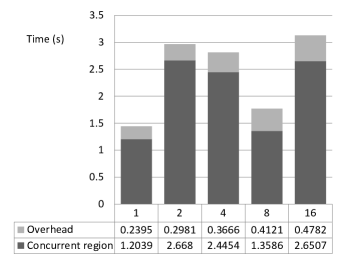
Figure 6: The CPU/GPU concurrent region time vs the overhead (data transfer between the nodes and CPU/GPU sequential region) of the FMM algorithm for 2 GPUs per node. The testing case size increases proportionally to the number of nodes (8M particles per node).

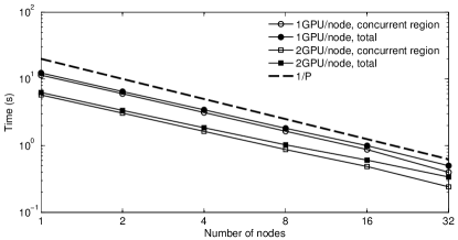
Figure 7: The results of the strong scalability test for 1 and 2 GPUs per node of the testing cluster. The thick dashed line shows perfect scalability $t=O\left(1/P\right)$. The problem size is fixed to be 16M.

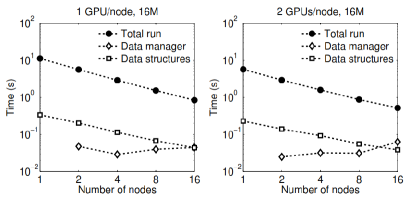
Figure 8: The data manager and data structure processing time against the total run time. The problem sizes are fixed to be 16M running on 1 to 16 nodes. Each node uses 1 (left) or 2 (right) GPUs. The time is measured for potential only computations.

We used a small cluster (“Chimera”) at the University of Maryland for tests, which has 32 nodes interconnected via Infiniband. Each node was composed of a dual socket quad-core Intel Xeon X5560 2.8 GHz CPUs, 24 GB of RAM  and two Tesla C1060 GPUs. We define concurrent region here as the period when the GPU(s) computes local summation and the CPU cores compute translation simultaneously. In all tests we used the FMM for the Laplace equation in 3D, $\Phi(\mathbf{y},\mathbf{x})=1/|\mathbf{y}-\mathbf{x}|$ (see [33]).

First, the weak scalability of our algorithm was tested by fixing the number of particles per node to $N/P=2^{23}$ and varying the number of nodes. In Fig. 6, we show our overhead vs. concurrent region time against the baseline algorithm performance. For perfect parallelization/scalability, the run time in this case should be constant. In practice, we observed an oscillating pattern with slight growth of the average time. In [31], two factors were explained which affect the perfect scaling: reduction of the parallelization efficiency of the CPU part of the algorithm and the data transfer overheads, which also applies to our results. With the box type information, we could fully distribute all the translations among nodes and avoid the unnecessary duplication of the data structure, which would become significant at large sizes. Since our import/export data of each node only relates to the boundary surfaces, we improve the deficiency of their simplified algorithm that also shows up in the data transfer overheads, which increases with $l_{\max}$.

In Fig. 6, the full FMM algorithm shows almost the same CPU/GPU concurrent region time for the cases with similar particle density (the average number of particles in a spatial box at $l_{max}$).Moreover, the overheads of this algorithm only slightly increases in contrast to the big jump seen the baseline algorithm when $l_{max}$ changes. Even though the number of particles on each node remains the same, the problem size increases hence results in the deeper octree and more spatial boxes to handle, which also contributes to such overhead increase (besides communication cost). Nevertheless, it could improve the overall algorithm performance and its weak scalability by using these new data structures.

Second, we also performed the strong scalability test, in which $N$ is fixed and $P$ is changing (Fig. 7). The tests were performed for $N=2^{23},2^{24}$ and $P=1,2,4,8,16,32$ with one and two GPUs per node. Even though, our algorithm demonstrates superior scalability compared with the baseline algorithm, we still observe the slight deviations from the perfect scaling for the 8M case. For 16M case, the total run time of both 1 and 2 GPU shows the well scaling because the GPU work was a limiting factor of CPU/GPU concurrent region (the dominant cost). This is consistent with the fact that the sparse MVP alone is well scalable. For 8M case, in the case of two GPUs, the CPU work was a limiting factor for the parallel region. However, we can see approximate correspondence of the times obtained for two GPUs/node to the ones with one GPU/node, i.e. doubling of the number of nodes with one GPU or increasing the number of GPUs results in approximately the same timing. This shows a reasonably good balance between the CPU and GPU work in the case of 2 GPUs per node, which implies this is more or less the optimal configuration for a given problem size.

Finally, we validated the acceptable cost of the communication scheme and the computation of box type. There is a data manager in our multiple node FMM algorithm, which is used to manage the box import/export and communications. So we can compare this data manager processing time (including M-data exchange) and the overall data structure construction time with the total running time in Fig. 8. Given the problem size and truncation number fixed, our communication increases as the number of nodes (roughly $P^{1/3}$ in Eq. 7). In our strong scalability tests, such time is in the order of 0.01 seconds while the wall clock time is in the order of 1 or 0.1 seconds (contribute $1\%\sim 15\%$ of overall time), even though GPUs are not fully occupied in some cases. This implies such cost can be neglected in larger problems, in which the kernel evaluations keep all GPUs fully loaded. Our implementation incorporate the box type computation with other data structures, such as octree and translation neighbors, hence it makes more sense to report the total data structure cost. From Fig. 8 we observe that our data structure time decrease similarly as the wall clock time (as $1/P$) and shows good strong scalability.

However, it could be problematic if each node is only assigned a small number of boxes, which would occur given a large number of nodes. Eventually the subdivision of the domain would result in the number of boxes in the boundary region of each sub-domain is more or less the same as that of domain itself. In this case, the number of boxes to exchange is almost the same as the total global spatial boxes. Note that although the data manager processes the box data searching and consolidating, its main cost comes from the communication but not those processing. Hence, all the traffic (each box has $2p^{2}$ coefficients) that must go through the master node will become the bottleneck of the entire system. However, this communication traffic issue is intrinsic to the splitting of the global octree. One possible mitigation might be implementing a many-to-many communication model. In fact, in our current implementation, each node is capable of computing the sending or requesting address (node IDs) of each export or import box and this further improvement by investigating communication cost is left for future work.

5 Conclusion

For the single-node FMM, we are able to device a new algorithm, which also has the advantage that it achieves the FMM data structure in $O(N)\;$time, bringing the overall complexity of the FMM to this level for a given accuracy. Comparison of the GPU and CPU times for the same algorithm show accelerations in the range 20-100 times. This shows the feasibility of the use of GPUs for data structure construction, which satisfyingly reduce the data-structure step to a small part of the FMM overall computation time. The multiple node data structures developed here can handle non-uniform distributions and achieve workload balance. We developed parallel algorithms to determine the import and export boxes in which the granularity is spatial boxes. Their parallel GPU implementations are shown to have very small overhead and good scalability.

Acknowledgements

Work partially supported by AFOSR under MURI Grant W911NF0410176 (PI Dr. J. G. Leishman, monitor Dr. D. Smith); in addition NG was partially supported by Grant G34.31.0040 (PI Dr. I. Akhatov) of the Russian Ministry of Education & Science. We acknowledge NSF award 0403313 and NVIDIA for the Chimera cluster at the CUDA Center of Excellence at UMIACS. Work also partially supported by Fantalgo, LLC;

References

- [1] L. Nyland, M. Harris, J. Prins, Fast n-body simulation with cuda, in: H. Nguyen (Ed.), GPU Gems 3, Addison Wesley Professional, 2007, Ch. 31, pp. 677–695.
- [2] A. Gualandris, S. P. Zwart, A. Tirado-Ramos, Performance analysis of direct n-body algorithms for astrophysical simulations on distributed systems, Parallel Comput. 33 (2007) 159–173.
- [3] L. Greengard, V. Rokhlin, A fast algorithm for particle simulations, J. Comput. Phys. 73 (1987) 325–348.
- [4] J. Barnes, P. Hut, A hierarchical O(N log N) force-calculation algorithm, Nature 324 (6096) (1986) 446–449.
- [5] T. Darden, D. York, L. Pedersen, Particle mesh Ewald: An method for Ewald sums in large systems, J. Chem. Phys. 98 (12) (1993) 10089–10092.
- [6] H. Samet, Foundations of Multidimensional and Metric Data Structures (The Morgan Kaufmann Series in Computer Graphics and Geometric Modeling), Morgan Kaufmann Publishers Inc., San Francisco, CA, USA, 2005.
- [7] R. J. Anderson, Tree data structures for n-body simulation, SIAM J. Comput. 28 (6) (1999) 1923–1940.
- [8] J. Dongarra, F. Sullivan, Guest editors’ introduction: the top 10 algorithms, Computing in Science and Engineering 2 (2000) 22–23.
- [9] J. Bédorf, E. Gaburov, S. Portegies Zwart, A sparse octree gravitational N-body code that runs entirely on the GPU processor, Journal of Computational Physics 231 (7) (2012) 2825–2839.
- [10] M. Harris, S. Sengupta, J. D. Owens, Parallel prefix sum (scan) with CUDA, in: H. Nguyen (Ed.), GPU Gems 3, Addison Wesley, 2007, Ch. 39, pp. 851–876.
- [11] Q. Hu, M. Syal, N. A. Gumerov, R. Duraiswami, J. G. Leishman, Toward improved aeromechanics simulations using recent advancements in scientific computing, in: Proceedings 67th Annual Forum of the American Helicopter Society, 2011.
- [12] P. Ajmera, R. Goradia, S. Chandran, S. Aluru, Fast, parallel, gpu-based construction of space filling curves and octrees, in: Proceedings of the 2008 symposium on Interactive 3D graphics and games, I3D ’08, ACM, New York, NY, USA, 2008, pp. 10:1–10:1.
- [13] N. A. Gumerov, R. Duraiswami, Fast Multipole Methods for the Helmholtz Equation in Three Dimensions, Elsevier, Oxford, 2004.
- [14] G. M. Morton, A computer oriented geodetic data base and a new technique in file sequencing, in: IBM Germany Scientific Symposium Series, 1966.
- [15] N. A. Gumerov, R. Duraiswami, Y. A. Borovikov, Data structures, optimal choice of parameters, and complexity results for generalized multilevel fast multipole methods in dimensions, Tech. Rep. CS-TR-4458; UMIACS-TR-2003-28, University of Maryland Department of Computer Science and Institute for Advanced Computer Studies (April 2003).
- [16] F. E. Sevilgen, S. Aluru, A unifying data structure for hierarchical methods, in: Proceedings of the 1999 ACM/IEEE conference on Supercomputing (CDROM), Supercomputing ’99, ACM, New York, NY, USA, 1999.
- [17] B. Hariharan, S. Aluru, Efficient parallel algorithms and software for compressed octrees with applications to hierarchical methods, Parallel Comput. 31 (2005) 311–331.
- [18] L. Greengard, W. D. Gropp, A parallel version of the fast multipole method, Computers & Mathematics with Applications 20 (7) (1990) 63–71.
- [19] J. P. Singh, C. Holt, J. L. Hennessy, A. Gupta, A parallel adaptive fast multipole method, in: Proceedings of the 1993 ACM/IEEE conference on Supercomputing, Supercomputing ’93, ACM, New York, NY, USA, 1993, pp. 54–65.
- [20] H. Mahawar, V. Sarin, A. Grama, Parallel performance of hierarchical multipole algorithms for inductance extraction, in: Proceedings of the 11th international conference on High Performance Computing, HiPC’04, Springer-Verlag, Berlin, Heidelberg, 2004, pp. 450–461.
- [21] L. Ying, G. Biros, D. Zorin, H. Langston, A new parallel kernel-independent fast multipole method, in: Proceedings of the 2003 ACM/IEEE conference on Supercomputing, SC ’03, ACM, New York, NY, USA, 2003, pp. 14–30.
- [22] R. Yokota, T. Narumi, R. Sakamaki, S. Kameoka, S. Obi, K. Yasuoka, Fast multipole methods on a cluster of gpus for the meshless simulation of turbulence, Computer Physics Communications 180 (11) (2009) 2066–2078.
- [23] I. Lashuk, A. Chandramowlishwaran, H. Langston, T. Nguyen, R. Sampath, A. Shringarpure, R. Vuduc, L. Ying, D. Zorin, G. Biros, A massively parallel adaptive fast-multipole method on heterogeneous architectures, in: Proceedings of the Conference on High Performance Computing Networking, Storage and Analysis, SC ’09, ACM, New York, NY, USA, 2009, pp. 58:1–58:12.
- [24] S. Teng, Provably good partitioning and load balancing algorithms for parallel adaptive n-body simulation, SIAM J. Sci. Comput. 19 (1998) 635–656.
- [25] F. A. Cruz, M. G. Knepley, L. A. Barba, PetFMM—a dynamically load-balancing parallel fast multipole library, International Journal for Numerical Methods in Engineering 85 (4) (2011) 403–428.
- [26] D. B. Kirk, W. Hwu, Programming Massively Parallel Processors: A Hands-on Approach, 1st Edition, Morgan Kaufmann Publishers Inc., San Francisco, CA, USA, 2010.
- [27] NVIDIA, NVIDIA CUDA C Programming Guide, 3rd Edition (2010).
- [28] NVIDIA, OpenCL Programming Guide for the CUDA Architecture, 3rd Edition (2010).
- [29] N. A. Gumerov, R. Duraiswami, Fast multipole methods on graphics processors, J. Comput. Phys. 227 (18) (2008) 8290–8313.
- [30] G. Blelloch, Scans as primitive parallel operations, IEEE Transactions on Computers 38 (1987) 1526–1538.
- [31] Q. Hu, N. A. Gumerov, R. Duraiswami, Scalable fast multipole methods on distributed heterogeneous clusters, in: Proceedings of the Conference on High Performance Computing Networking, Storage and Analysis, SC ’11, ACM, Seattle, WA, USA, 2011, pp. 1–12.
- [32] Q. Hu, N. A. Gumerov, R. Duraiswami, Scalable distributed fast multipole methods, in: Proceedings of the 14th International Conference on High Performance Computing and Communications (HPCC-2012), HPCC ’12, ACM, 2012.
- [33] N. A. Gumerov, R. Duraiswami, Fast multipole method for the biharmonic equation in three dimensions, J. Comput. Phys. 215 (1) (2006) 363–383.