Multiple dynamic transitions in nonequilibrium work fluctuations

Abstract

The time-dependent work probability distribution function $P(W)$ is investigated analytically for a diffusing particle trapped by an anisotropic harmonic potential and driven by a nonconservative drift force in two dimensions. We find that the exponential tail shape of $P(W)$ characterizing rare-event probabilities undergoes a sequence of dynamic transitions in time. These remarkable locking-unlocking type transitions result from an intricate interplay between a rotational mode induced by the nonconservative force and an anisotropic decaying mode due to the conservative attractive force. We expect that most of high-dimensional dynamical systems should exhibit similar multiple dynamic transitions.

Systems in thermal equilibrium are governed by the principle of statistical mechanics. It serves as the unified framework for the study of thermodynamic properties of equilibrium systems, and has been successful since it was established centuries ago. On the contrary, such a principle, except for the second law of thermodynamics, was absent for nonequilibrium systems, which made it difficult to understand nonequilibrium phenomena. Recently, discovery of the fluctuation theorem opened a new perspective on nonequilibrium processes and has attracted a lot of interests Seifert12 . The fluctuation theorem refers to identity relations for a thermodynamic quantity, such as work, heat, or entropy production, that are derived theoretically for a wide class of nonequilibrium process Evans93 ; Gallavotti ; Jarzynski97 ; Crooks99 ; Lebowitz99 ; Hatano01 ; Seifert05 ; Kurchan07 ; Sevick08 ; Noh12 , and are also confirmed experimentally Carberry04 ; Reid04 ; Collin05 ; Garnier05 ; Ciliberto10 ; Hayashi10 . It not only serves as a criterion diagnostic to nonequilibrium, but also sheds light on quantitative understanding of nonequilibrium fluctuations Harada05 ; Seifert06 ; Blickle07 ; Prost09 ; Mallick11 .

The fluctuation theorem evokes the importance of studying nonequilibrium fluctuations, especially in the rare-event region. Many studies have been done for the probability distribution functions (PDF’s) of the work and heat associated with nonequilibrium processes, theoretically and experimentally Evans93 ; Gallavotti ; Jarzynski97 ; Crooks99 ; Lebowitz99 ; Hatano01 ; Seifert05 ; Kurchan07 ; Sevick08 ; Noh12 ; Carberry04 ; Reid04 ; Collin05 ; Garnier05 ; Ciliberto10 ; Kwon11 ; Filliger07 ; JS02 ; Evans02 ; Zon03 ; Ciliberto ; Ciliberto13 . These are to confirm the fluctuation theorem in the first place, and then to investigate the nature of nonequilibrium fluctuations. Normally it is a formidable task to find the PDF analytically for a specific nonequilibrium process, so most studies are limited to special cases such as the large deviation study in the infinite-time limit Farago02 ; Fogedby11 ; Visco06 ; Puglisi06 .

In this Letter, we investigate the PDF of a nonequilibrium work $W$ over a finite time interval $t$ in a two-dimensional linear diffusion system (LDS), driven by a nonconservative linear drift force. The LDS is often referred to as a multivariate Ornstein-Uhlenbeck process describing the motion of a Brownian particle trapped by a linear force in the overdamped limit Gardiner ; Risken . It is also well known that the LDS serves as a generic model to describe the fluctuation effects on deterministic dynamic solutions of general nonlinear systems in the context of the van Kampen’s system size expansion Gardiner . Experimental systems described by the LDS are so diverse, including a nano heat engine in contact with multiple heat reservoirs Filliger07 , a colloidal particle driven along periodic potential imposed by laser traps Blickle07 , biological molecular motor systems Hayashi10 , electric circuits Ciliberto13 , global climate systems Weiss , and musical instruments Gannot .

The LDS is simple enough that the PDF $P(W)$ is analytically tractable for finite time interval. Our study reveals that even such a simple system displays a surprisingly rich dynamic behavior with a sequence of dynamic transitions in time. We briefly summarize the results with dimensionless $W$: (i) The PDF has exponential tails with power-law prefactors as $P(W)\sim|W|^{-\alpha_{\pm}}\ e^{-W/W_{\pm}}$ for large $|W|$. The power-law exponents are the same in both sides ($\alpha_{+}=\alpha_{-}=\alpha$), and the characteristic works $W_{+}>0$ and $W_{-}<0$ satisfy $1/W_{+}+1/W_{-}=-1$, which are required by the detailed fluctuation theorem Crooks99 ; Reid04 ; Kwon11 . (ii) The power-law exponent $\alpha$ can take three different values of $0$, $1/2$, and $2$. Accordingly, the PDF is categorized into type 0 with $\alpha=0$, type I with $\alpha=1/2$, and type II with $\alpha=2$. Interestingly, $W_{\pm}$ continuously varies with time $t$ for type 0 and type I, while they are constants of time for type II. (iii) Typically, the system undergoes a dynamic transition from type I to type II as $t$ increases. The characteristic work $W_{+}$ increases smoothly with $t$ and suddenly becomes frozen at the transition time $t_{c}$ and afterwards. This is a kind of a locking transition. More remarkably, in some parameter space, the PDF alternates between type I and type II indefinitely, i.e. infinite number of locking-unlocking type transitions. In general, a finite sequence of dynamic transitions is also possible as well as no transition with type I in all time. Type 0 is found without any dynamic transition, only in a special case.

We consider a LDS with the equations of motion

$$\frac{d{\bm{q}}}{dt}=-{\mathsf{F}}\cdot{\bm{q}}+{\bm{\xi}}$$ (1)

where ${\bm{q}}=({q}_{1},\cdots,{q}_{d})^{T}$ is a $d$-dimensional vector, ${\mathsf{F}}=({F}_{ij})$ is a constant positive-definite $(d\times d)$ force matrix, and ${\bm{\xi}}(t)=({\xi}_{1}(t),\cdots,{\xi}_{d}(t))^{T}$ is the Langevin noise satisfying

$$\langle{\xi}_{i}(t)\rangle=0\ ,\ \langle{\xi}_{i}(t){\xi}_{j}(t)\rangle=2{D}_{ij}\delta(t-t^{\prime})$$ (2)

with a noise correlation matrix $\mathsf{D}=({D}_{ij})$ which is symmetric and positive-definite. After a similarity and a scale transformation, one can take the noise matrix as the identity matrix $\mathsf{I}$ ($\mathsf{D}=\mathsf{I}$) without loss of generality.

The force matrix can be decomposed into the conservative and nonconservative parts as $\mathsf{F}={\mathsf{F}}_{c}+{\mathsf{F}}_{nc}$ with symmetric ${\mathsf{F}}_{c}=\mathsf{F}_{c}^{T}$ and nonsymmetric ${\mathsf{F}}_{nc}$. When ${\mathsf{F}}_{nc}=0$, the total force ${\bm{f}}=-\mathsf{F}\cdot{\bm{q}}=-{\mathsf{\nabla}}V({\bm{q}})$ is conservative with a potential function $V({\bm{q}})=\frac{1}{2}{\bm{q}}^{T}\cdot\mathsf{F}\cdot{\bm{q}}$. The steady-state PDF is given by the equilibrium Boltzmann distribution $P_{eq}({\bm{q}})\propto e^{-V({\bm{q}})}$. A nonsymmetric force matrix (${\mathsf{F}}_{nc}\neq\mathsf{0}$) indicates the presence of a nonconservative force $\bm{f}_{nc}=-{\mathsf{F}}_{nc}\cdot\bm{q}$ which cannot be written as a gradient function. It drives the system out of equilibrium. Here, we only consider the antisymmetric ${\mathsf{F}}_{nc}$ ($=-{\mathsf{F}}_{nc}^{T}$) for simplicity exp .

Suppose that the system is prepared in the thermal equilibrium with $P_{eq}({\bm{q}})\propto e^{-({1/2}){\bf q}^{T}\cdot{\mathsf{F}}_{c}\cdot{\bm{q}}}$ with the conservative force $\bm{f}_{c}=-{\mathsf{F}}_{c}\cdot\bm{q}$ only, then turn on the nonconservative force $\bm{f}_{nc}$ at $t=0$. The nonequilibrium work (done by $\bm{f}_{nc}$) on the particle following a path ${\bm{q}}(\tau)$ for $0\leq\tau\leq t$ is given by

$$\mathcal{W}[{\bm{q}}(\tau)]=-\int_{0}^{t}d\tau\ \frac{d{\bm{q}}(\tau)^{T}}{d\tau}\cdot{\mathsf{F}}_{nc}\cdot\bm{q}(\tau)\ .$$ (3)

We are interested in the PDF $P(W)=\langle\delta(W-\mathcal{W}[{\bm{q}(\tau})])\rangle$ and its characteristic function $\mathcal{G}(t;\lambda)=\langle e^{-\lambda W}\rangle=\int dWe^{-\lambda W}P(W)$, which should satisfy the fluctuation theorem symmetry as $P(W)/P(-W)=e^{W}$ and consequently ${\mathcal{G}}(\lambda)={\mathcal{G}}(1-\lambda)$ Kwon11 .

The characteristic function can be written as a path integral ${\mathcal{G}}(\lambda)\propto\int D[{\bm{q}}]e^{-L[{\bm{q}};\lambda]}$ with an action $L$. In our previous work Kwon11 , we developed a formalism evaluating the path integral for the LDS where the action $L$ is quadratic in ${\bm{q}}$. The key idea is described as below. The Gaussian integration can be performed successively from ${\bm{q}}(0)$ to ${\bm{q}}(t)$ at discretized times. Integration up to ${\bm{q}}(\tau)$ yields a modified kernel for ${\bm{q}}(\tau+\Delta t)$, denoted by a symmetric $d\times d$ matrix $\widetilde{\mathsf{A}}(\tau+\Delta\tau;\lambda)$. Comparing the kernels at $\tau$ and $\tau+\Delta\tau$ and taking the limit $\Delta\tau\to 0$, one can derive the differential equation for the kernel $\widetilde{\mathsf{A}}(\tau)$ as

$$\frac{d}{d\tau}\tilde{\mathsf{A}}(\tau;\lambda)=-2\tilde{\mathsf{A}}^{2}+\tilde{\mathsf{A}}\tilde{\mathsf{F}}+\tilde{\mathsf{F}}^{T}\tilde{\mathsf{A}}+\bm{\Lambda}$$ (4)

with the initial condition $\tilde{\mathsf{A}}(0)={\mathsf{F}}_{c}$ and the auxiliary matrices $\tilde{\mathsf{F}}(\lambda)=\mathsf{F}-2\lambda{\mathsf{F}}_{nc}$ and $\bm{\Lambda}(\lambda)=(\mathsf{F}^{T}\mathsf{F}-\tilde{\mathsf{F}}^{T}\tilde{\mathsf{F}})/2$. The characteristic function is then given by the product of Gaussian integrals with the kernel $\widetilde{\mathsf{A}}(\tau)$ along the path ${\bm{q}}(\tau)$, which yields

$$\ln\mathcal{G}(t;\lambda)=-\int_{0}^{t}d\tau\ {\rm Tr}(\tilde{\mathsf{A}}(\tau;\lambda)-\tilde{\mathsf{F}})-\frac{1}{2}\ln\frac{\det\tilde{\mathsf{A}}(t;\lambda)}{\det{\mathsf{F}}_{c}}.$$ (5)

We apply the formalism to a two-dimensional system with the force matrices, parameterized as comment

$${\mathsf{F}}_{c}=\left(\begin{array}[]{cc}1+u&0\\ 0&1-u\end{array}\right),\ \mathsf{F}_{nc}=\left(\begin{array}[]{cc}o&\ \varepsilon\\ -\varepsilon&\ 0\end{array}\right)\ .$$ (6)

One can set the trace of F to any positive number by the global rescaling of ${\bm{q}}$ and $t$. Here, it is set to be $2$. Positive-definiteness of $\mathsf{F}$ and ${\mathsf{F}}_{c}$ requires that $u^{2}<1$. The system describes a Brownian particle trapped by an anisotropic harmonic potential and driven by a rotational torque. The parameter $\varepsilon$ corresponds to the strength of nonequilibrium driving (torque), while the parameter $u$ represents the anisotropy of the harmonic potential.

Before considering the general case, we present the solution in the special isotropic case with $u=0$. In this case, the matrix $\tilde{\mathsf{A}}$ is proportional to the identity matrix as $\tilde{\mathsf{A}}=z(\tau;\lambda)\ {\mathsf{I}}$. Then, Eq. (4) becomes ${dz}/{d\tau}=-2z^{2}+2z+2\varepsilon^{2}\lambda(1-\lambda)$ with $z(0)=1$ and Eq. (5) is written as

$$\ln\mathcal{G}(t;\lambda)=-2\int_{0}^{t}(z(\tau;\lambda)-1)d\tau-\ln z(t;\lambda)\ .$$ (7)

The solution of the differential equation is given by

$$z(\tau;\lambda)=\frac{1}{2}\left(1+\sqrt{\Delta}\frac{1+\sqrt{\Delta}\tanh(\sqrt{\Delta}\tau)}{\sqrt{\Delta}+\tanh(\sqrt{\Delta}\tau)}\right)$$ (8)

with $\Delta(\lambda)\equiv 1-4\varepsilon^{2}\lambda(\lambda-1)$. Inserting Eq. (8) into Eq. (7), we obtain ${\mathcal{G}}(t;\lambda)$ and draw the following conclusions: (i) Since $\Delta(\lambda)=\Delta(1-\lambda)$, one finds $\mathcal{G}(t;\lambda)=\mathcal{G}(t;1-\lambda)$ at all $t$. This verifies the fluctuation theorem. (ii) Given $t$, there exists $\lambda_{0}(t)>1$ such that $z(t;\lambda=\lambda_{0})=z(t;\lambda=1-\lambda_{0})=0$. The logarithmic term in Eq. (7) indicates simple poles of $\mathcal{G}(t;\lambda)$ at $\lambda=\lambda_{0}$ and $1-\lambda_{0}$. (iii) The simple poles manifest the exponential tails of $P(W)$:

$$P(W)\sim\left\{\begin{array}[]{ll}e^{-(\lambda_{0}(t)-1)W}&,\ W\to\infty\\[5.69054pt] e^{-\lambda_{0}(t)|W|}&,\ W\to-\infty\end{array}\right.$$ (9)

with $\lambda_{0}(t)$ monotonically decreasing in $t$ and asymptotically approaching $\lambda_{c}=\frac{1}{2}+{\sqrt{1+\varepsilon^{2}}}/{(2\varepsilon)}\geq 1$. This PDF belongs to type 0.

The analysis above gives us a lesson that the singularity of $\mathcal{G}$, hence the tail behavior of $P(W)$, is determined from the root of $\det\tilde{\mathsf{A}}(t;\lambda)=0$. In the isotropic potential case ($u=0$), two eigenvalues of $\tilde{\mathsf{A}}$ are degenerate. So, the root contributes to a simple pole of $\mathcal{G}$ and the pure exponential tail of $P(W)$. When the degeneracy is broken, which is the case for an anisotropic potential with $u\neq 0$, $\mathcal{G}$ has a square-root singularity and one may simply expect the PDF of type I. However, the actual behavior turns out to be much richer. The particle driven by the torque undergoes an energy barrier periodic in the azimuthal direction, due to the anisotropy in the potential. Therefore there emerges an extra time scale to overcome the barrier in addition to the overall relaxation time. Their interplay can be understood from the full solution of Eq. (4).

Here, we sketch briefly the way to find the exact solution of Eq. (4). First, note that the inhomogeneous quadratic differential equation, Eq. (4), can be transformed into a solvable homogeneous linear differential equation by shifting and inverting $\mathsf{\tilde{A}}(\tau;\lambda)$ such as

$$\mathsf{\tilde{A}}(\tau;\lambda)\equiv\mathsf{\tilde{A}}_{s}(\lambda)+\mathsf{R}(\tau;\lambda)^{-1}\ ,$$ (10)

where $\tilde{\mathsf{A}}_{s}(\lambda)$ is the fixed-point solution satisfying $d\tilde{\mathsf{A}}/{d\tau}|_{\tilde{\mathsf{A}}=\tilde{\mathsf{A}}_{s}}=\mathsf{0}$. Then, it is straightforward to derive

$$\frac{d\mathsf{R}}{d\tau}=2\mathsf{I}-\mathsf{R\hat{F}^{T}-\hat{F}R}\ ,$$ (11)

where $\hat{\mathsf{F}}(\lambda)\equiv\tilde{\mathsf{F}}(\lambda)-2\tilde{\mathsf{A}}_{s}(\lambda)$. Its solution is given as

$$\mathsf{R}(\tau;\lambda)=e^{-\tau\hat{\mathsf{F}}}\ \mathsf{R}(0;\lambda)\ e^{-\tau\hat{\mathsf{F}}^{T}}+2\int_{0}^{\tau}d\tau^{\prime}e^{-\tau^{\prime}\hat{\mathsf{F}}}e^{-\tau^{\prime}\hat{\mathsf{F}}^{T}}.$$ (12)

In two dimensions, the explicit expression for Eq. (10) is available. It is rather complex, and will be presented elsewhere Noh11 .

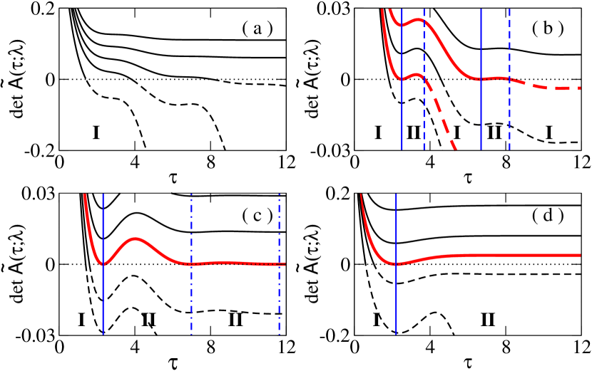
Figure 1: (Color online) Time evolution of $\det\tilde{\mathsf{A}}(\tau;\lambda)$ when $\varepsilon=3/10$ and (a) $u=0.65$, (b) $0.7$, (c) $u^{*}=\sqrt{109/200}$, and (d) $0.8$ with several values of $\lambda>1$ (lower curves represent larger values of $\lambda$). The curves tangential to the $\tau$ axis (dotted horizontal line) are drawn with thick lines (red). The characteristic function $\mathcal{G}$ is well defined only when $\det\tilde{\mathsf{A}}>0$. Curves in the unphysical regions with $\det\tilde{\mathsf{A}}<0$ are plotted with dashed lines.

The solution is the starting point for further analysis of the PDF. We found that $\det{\tilde{\mathsf{A}}(t;\lambda)}$ exhibits a complex behavior depending on values of $\varepsilon$ and $u$. There are four distinct cases, which are shown in Fig. 1. The plots are obtained for a few values of $u$ to a given $\varepsilon=3/10$.

(i) When $u$ (anisotropy) is small enough (see Fig. 1(a)), the curve is not tangential to the $\tau$ axis at any value of $\lambda$. For any given $\tau=t$, one can find $\lambda_{0}$ such that $\det\tilde{\mathsf{A}}(\tau,\lambda_{0})=0$ (non-degenerate root). Then, $\det\tilde{\mathsf{A}}(t,\lambda)\sim(\lambda_{0}-\lambda)$ near $\lambda\simeq\lambda_{0}$ and, from Eq. (5), $\mathcal{G}(t,\lambda)\sim(\lambda_{0}-\lambda)^{-1/2}$. Hence, the PDF has a tail $P(W)\sim|W|^{-1/2}e^{\lambda_{0}W}$ in the $W\to-\infty$ limit (type I), with $\lambda_{0}=\lambda_{0}(t)$ monotonically decreasing with $t$ to an asymptotic value $\lambda_{c}(u,\varepsilon)>1$.

(ii) In the intermediate values of $u$ (see Fig. 1(b)), the curve is tangential to the $\tau$ axis at multiple values of $\lambda$. We will denote the time for the $n$-th tangential point as $t_{n}^{+}$ (marked with vertical solid lines) and the corresponding $\lambda$ value as $\lambda_{n}$. The curve, $\det\tilde{\mathsf{A}}(\tau,\lambda_{n})$, that is tangential at $\tau=t_{n}^{+}$ may cross the $\tau$ axis at a later time denoted as $\tau=t_{n}^{-}$ (marked with vertical dashed lines). This crossing is linear (non-degenerate root) and never happens again later. Within the time interval $t_{n}^{+}<t<t_{n}^{-}$, the characteristic function $\mathcal{G}(t;\lambda)$ is finite for $\lambda<\lambda_{n}$, and then it diverges discontinuously at $\lambda=\lambda_{n}$. Hence the PDF has a tail $P(W)\sim|W|^{-2}e^{\lambda_{n}W}$ in the $W\to-\infty$ limit (type II) exp2 . Note that $\lambda_{n}$ is a constant of time within the finite time interval. Outside the interval, the PDF belongs to type I. Hence, the PDF alternates between type I and type II many times as $t$ increases.

(iii) At the special value of $u=u^{*}\equiv\sqrt{(1+\varepsilon^{2})/2}$, the curve, $\det\tilde{\mathsf{A}}(\tau,\lambda^{*})$, with $\lambda^{*}=(1+\varepsilon)/(2\varepsilon)$ is tangential to the $\tau$ axis infinitely many times as

$$\det\tilde{\mathsf{A}}(\tau;\lambda^{*})=\frac{\varepsilon(1-\varepsilon)(1+\varepsilon)\left(1+\cos\omega\tau\right)}{4\left(e^{2\varepsilon\tau}-\frac{1-\varepsilon}{1+\varepsilon}-\varepsilon\frac{1-\varepsilon}{1+\varepsilon}\cos\omega\tau\right)}\ ,$$ (13)

with $\omega=\sqrt{2(1-\varepsilon^{2})}$ and the tangential points at $t_{n}^{+}=(2n-1)\pi/\omega$ $(n=1,2,\ldots)$. Note that $t_{n}^{-}=t_{n+1}^{+}$. Hence, the PDF belongs to type I when $t<t_{1}^{+}$ (marked with the vertical solid line) and changes to type II afterwards except periodic instantaneous moments at $t=t_{n}^{+}$ ($n\geq 2$) (marked with vertical dot-dashed lines).

(iv) When $u>u^{*}$, the curve is tangent to the $\tau$ axis at a single value of $\lambda$ at $\tau=t_{1}^{+}$ (marked with the vertical solid line) without crossing the $\tau$ axis later. Hence, the PDF belongs to type I for $\tau<t_{1}^{+}$ and type II afterwards forever.

Our analysis reveals that the system undergoes a dynamic transition in the tail shape of the PDF between type I characterized by $P(W)\sim|W|^{-1/2}e^{\lambda_{0}W}$ and the type II characterized by $P(W)\sim|W|^{-2}e^{\lambda_{0}W}$ for large negative $W$. The same applies for large positive $W$ due to the fluctuation theorem symmetry. The parameter $\lambda_{0}$, which corresponds to the inverse of the characteristic fluctuation size $|W_{-}|$ for the negative PDF tail, decreases smoothly in time for type I, while it is locked for type II. For example, in case of (ii), $\lambda_{0}$ decreases up to $t=t_{1}^{+}$, and is locked for a while till $t=t_{1}^{-}$, then is unlocked and decreases again till $t=t_{2}^{+}$, and so on. These locking-unlocking transitions occur many times as $t$ goes by.

For given values of $u$ and $\varepsilon$, the time dependence of $\lambda_{0}(t)$ can be calculated numerically exactly from the roots of $\det\tilde{\mathsf{A}}(t;\lambda)=0$, using the solution given in Eq. (10). In Fig. 2, we plot $\lambda_{0}$ as function of $t$ for several values of $u$ at $\varepsilon=3/10$. When the anisotropy is weak (small $u$), the inverse characteristic work $\lambda_{0}(t)$ decreases smoothly with time (upper curves in Fig. 2). With the intermediate anisotropy, it decreases being locked for a while in multiple or infinite number of plateaus (middle curves). When the anisotropy is strong (large $u$), it decreases at small $t$ and then is locked to a constant value forever (lower curves). Consequently, the PDF undergoes a single dynamic transition for large values of $u$, infinitely many transitions for intermediate values of $u$, and no transition for small $u$. From the plots in Fig. 2, one can construct the phase diagram in the $u$-$t$ plane, which is drawn in Fig. 3. The phase diagram separates the regions with PDF of type I and type II. When the anisotropy is weak (strong), the system tends to display the PDF of type I (II). The phase boundary becomes complex in between, where multiple dynamic transitions can be observed in the system with intermediate anisotropy.

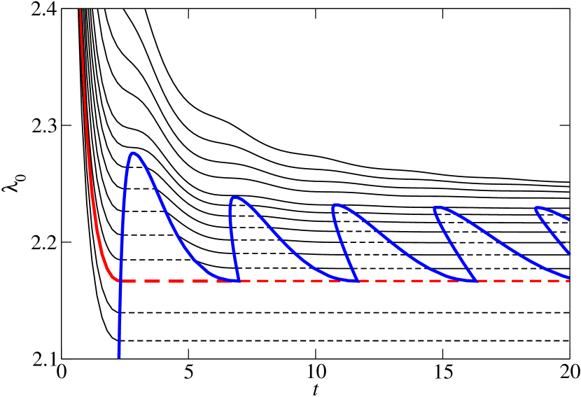
Figure 2: (Color online) Plots of $\lambda_{0}$ vs $t$ for several values of $u$ at $\varepsilon=3/10$. The value of $u$ ranges from $0.55$ (top) to $0.76$ (bottom). The solid curves correspond to the PDF of type I, while the dashed line corresponds to the PDF of type II with the boundary drawn with the thick zigzag (blue) curve. The thick (red) curve corresponds to the case with $u=u^{*}$.

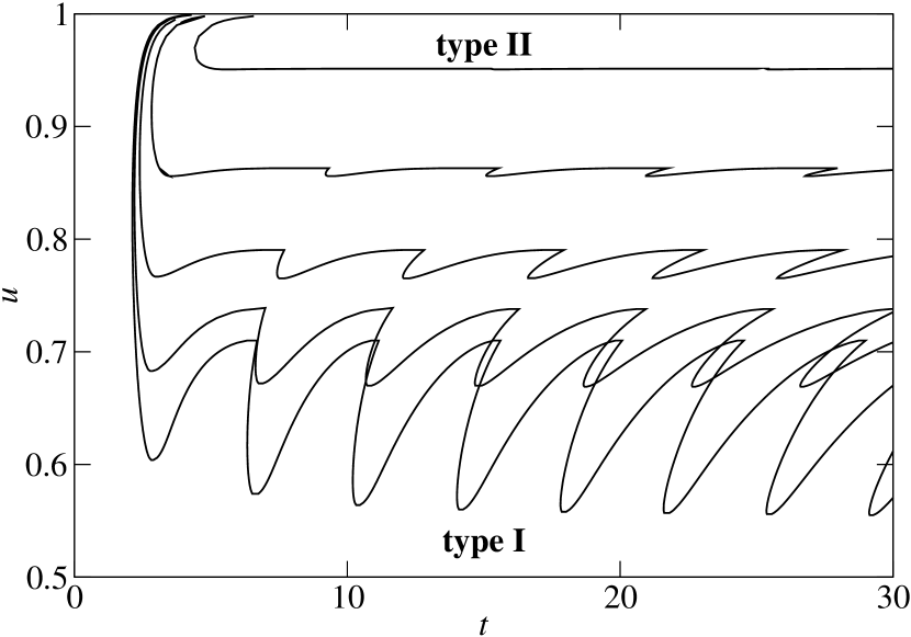
Figure 3: Phase diagram in the $u$-$t$ plane for several values of $\varepsilon=0.1$ (bottom), $0.3$, $0.5$, $0.7$, and $0.9$ (top). The PDF belongs to type II in the region surrounded by the phase boundary curve, and type I elsewhere except the line $u=0$ where the type-0 PDF is found. For $\varepsilon\geq 1$, the phase boundary disappears completely and no type II exists.

In summary, our analytic result shows that such a simple LDS exhibits surprisingly complex nonequilibrium fluctuations. It raises interesting questions for the mechanism of the dynamic transition. The conservative part of the drift force generates an anisotropic harmonic potential, which attracts the particle toward the origin. The nonconservative part acts like a torque, which drives the particle into a rotational motion. It is useful to introduce the polar coordinate to focus on the rotational dynamics separately. Then, the dynamics of the polar angle may be written down effectively as $d\phi/dt=a\sin\phi+b+\xi$, where the potential amplitude $a$ should be proportional to the anisotropy $\sigma$ and the constant driving force $b$ should be proportional to the strength of the nonconservative force $\varepsilon$. This is the equation of motion in a tilted periodic potential Blickle07 . For $a\ll b$ (small $\sigma$), the particle has no time to relax in the potential well and drifts down into the steady state with a constant velocity. So there is no extra time scale except for the relaxation into the steady state. Thus, we expect no dynamic transitions and type-I PDF forever. For $a\gg b$ (large $\sigma$), the particle sits at the potential well long enough and fully relaxes inside the well. Then, it can hop to the neighboring well due to the noise after a finite time, which can be determined by the noise strength. This additional time scale exists and may set the transition time $t_{1}^{+}$. As the particle relaxation in the first well is fully developed already, there will be no additional time scale needed for successive hoppings. Thus, we expect one dynamic transition from type-I to type-II PDF. When $a\approx b$ (intermediate $\sigma$), it needs additional time scales for successive hoppings with incomplete relaxations within each potential well, which leads to multiple dynamic transitions. The above argument provides a plausible understanding of existence of multiple time scales, but does not fully capture underlying mechanisms of dynamic locking-unlocking transitions. Since the radial component also fluctuates in our model, there are more possible complex routes to relax into the steady state. It is remarkable to find no smearing out of sharp dynamic transitions with fully locking states. We leave full intuitive physical understanding of these dynamic transitions for future works.

As can be seen in our analysis, the remarkable characteristics of multiple dynamic transitions should not be a pathological property of some special systems. Hence, we expect that any high-dimensional dynamical system driven by a nonconservative force should exhibit similar or more complex multiple dynamic transitions in a reasonably large parameter space. It would be interesting to observe these locking-unlocking features in experimental setups such as in Hayashi10 ; Blickle07 ; Filliger07 ; Ciliberto13 and also in direct numerical simulations of the Langevin equation. However, it demands extremely high-precision and time-dependent work PDF measurements in rare-event regimes.

H.P. thanks David Mukamel and Haye Hinrichsen for useful discussions. This work was supported by the Basic Science Research Program through the NRF Grant No. 2013R1A2A2A05006776(J.D.N.), 2013R1A1A2011079(C.K.), and 2013R1A1A2A10009722(H.P.).

References

- (1) U. Seifert, Rep. Prog. Phys. 75, 126001 (2012).
- (2) D. J. Evans, E. G. D. Cohen, and G. P. Morriss, Phys. Rev. Lett. 71, 2401 (1993).
- (3) G. Gallavotti and E. G. D. Cohen, Phys. Rev. Lett. 74, 2694 (1995).
- (4) C. Jarzynski, Phys. Rev. Lett. 78, 2690 (1997).
- (5) G. E. Crooks, Phys. Rev. E 60, 2721 (1999); ibid. 61, 2361 (2000).
- (6) J. Lebowitz and H. Spohn, J. Stat. Phys. 95, 333 (1999).
- (7) T. Hatano and S.-I. Sasa, Phys. Rev. Lett. 86, 3463 (2001).
- (8) U. Seifert, Phys. Rev. Lett. 95, 040602 (2005).
- (9) J. Kurchan, J. Stat. Mech.: Theor. Exp. 2007, P07005 (2007).
- (10) E. M. Sevick, R. Prabhakar, S. R. Williams, and D. J. Searles, Ann. Rev. Phys. Chem. 59, 603 (2008).
- (11) J. D. Noh and J.-M. Park, Phys. Rev. Lett. 108, 240603 (2012).
- (12) D. M. Carberry, J. C. Reid, G. M. Wang, E. M. Sevick, D. J. Searles, and D. J. Evans, Phys. Rev. Lett. 92, 140601 (2004).
- (13) J. C. Reid, D. M. Carberry, G. M. Wang, E. M. Sevick, D. J. Searles, and D. J. Evans, Phys. Rev. E 70, 016111 (2004).
- (14) D. Collin, F. Ritort, C. Jarzynski, S. B. Smith, I. Tinoco, and C. Bustamante, Nature 437, 231 (2005).
- (15) N. Garnier and S. Ciliberto, Phys. Rev. E 71, 060101 (2005).
- (16) S. Ciliberto, S. Joubaud, and A. Petrosyan, J. Stat. Mech. P12003 (2010).
- (17) K. Hayashi, H. Ueno, R. Iino, and H. Noji, Phys. Rev. Lett. 104, 218103 (2010).
- (18) T. Harada and S.-I. Sasa, Phys. Rev. Lett. 95, 130602 (2005).
- (19) T. Speck and U. Seifert, Europhys. Lett. 74, 391 (2006).
- (20) V. Blickle, T. Speck, C. Lutz, U. Seifert, and C. Bechinger, Phys. Rev. Lett. 98, 210601 (2007); T. Speck, V. Blickle, C. Bechinger, and U. Seifert, EPL 79, 30002 (2007).
- (21) J. Prost, J.-F. Joanny, and J. M. R. Parrondo, Phys. Rev. Lett. 103, 090601 (2009).
- (22) K. Mallick, M. Moshe, and H. Orland, J. Phys. A 44, 095002 (2011).
- (23) C. Kwon, J. D. Noh, and H. Park, Phys. Rev. E 83, 061145 (2011).
- (24) R. Filliger and P. Reimann, Phys. Rev. Lett. 99, 230602 (2007).
- (25) J. S. Lee, C. Kwon, and H. Park, Phys. Rev. E 87, 020104(R) (2013).
- (26) D. J. Evans and D. J. Searles, Adv. Phys. 51, 1529 (2002).
- (27) R. van Zon and E. G. D. Cohen, Phys. Rev. Lett. 91, 110601 (2003); Phys. Rev E 69, 056121 (2004).
- (28) R. van Zon, S. Ciliberto, and E. G. D. Cohen, Phys. Rev. Lett. 92, 130601 (2004); S. Ciliberto, S. Joubaud, and A. Petrosyan, J. Stat. Mech. P12003 (2010).
- (29) S. Ciliberto, A. Imparato, A. Naert, and M. Tanase, Phys. Rev. Lett. 110, 180601 (2013).
- (30) J. Farago, J. Stat. Phys. 107, 781 (2002).
- (31) H. C. Fogedby and A. Imparato, J. Stat. Mech. P05015 (2011).
- (32) P. Visco, J. Stat. Mech. P06006 (2006) .
- (33) A. Puglisi, L. Rondoni, and A. Vulpiani, J. Stat. Mech. P08010 (2006).
- (34) C.W. Gardiner, Stochastic Methods: A Handbook for the Natural and Social Sciences (Springer, Berlin, 2009).
- (35) H. Risken, The Fokker-Planck Equation: Methods of Solution and Applications (Springer, New York, 1989).
- (36) J. B. Weiss, Phys. Rev. E 76, 061128 (2007); Geophy. Res. Lett. 36, L10705 (2009).
- (37) R. Talmon, D. Kushnir, R. R. Coifman, I. Cohen, and S. Gannot, IEEE Transactions on Signal Processing, 60, 1159 (2012).
- (38) A nonconservative force matrix needs not be antisymmetric, in general (see Kwon11 ).
- (39) may have a nonzero symmetric offdiagonal element. But it can be set to be zero without loss of generality by a rotational coordinate transformation.
- (40) J. D. Noh, C. Kwon, H. Park, unpublished.
- (41) Detailed analysis of Type II can be found in Kwon11 .