Near-UV Absorption, Chromospheric Activity, and Star-Planet Interactions in the WASP-12 system.

Abstract

Extended gas clouds have been previously detected surrounding the brightest known close-in hot Jupiter exoplanets, HD 209458 b and HD 189733 b; we observed the distant but more extreme close-in hot Jupiter system, WASP-12, with HST. Near-UV (NUV) transits up to three times deeper than the optical transit of WASP-12 b reveal extensive diffuse gas, extending well beyond the Roche lobe. The distribution of absorbing gas varies between visits. The deepest NUV transits are at wavelength ranges with strong photospheric absorption, implying the absorbing gas may have temperature and composition similar to the stellar photosphere. Our spectra reveal significantly enhanced absorption (greater than $3\sigma$ below the median) at $\sim 200$ individual wavelengths on each of two HST visits; 65 of these wavelengths are consistent between the two visits, using a strict criterion for velocity matching which excludes matches with velocity shifts exceeding $\sim 20\,{\rm km\,s^{-1}}$. Excess transit depths are robustly detected throughout the inner wings of the Mg II resonance lines independently on both HST visits. We detected absorption in Fe II 2586Å, the heaviest species yet detected in an exoplanet transit. The Mg II line cores have zero flux, emission cores exhibited by every other observed star of similar age and spectral type are conspicuously absent. WASP-12 probably produces normal Mg II profiles, but the inner portions of these strong resonance lines are likely affected by extrinsic absorption. The required Mg⁺ column is an order of magnitude greater than expected from the ISM, though we cannot completely dismiss that possibility. A more plausible source of absorption is gas lost by WASP-12 b. We show that planetary mass loss can produce the required column. Our Visit 2 NUV light curves show evidence for a stellar flare. We show that some of the possible transit detections in resonance lines of rare elements may be due instead to non-resonant transitions in common species. We present optical observations and update the transit ephemeris.

1 Introduction

WASP-12 b is one of the most extreme of the hot Jupiter exoplanets: it orbits only one stellar diameter away from the photosphere of its late F type host star, and is thus one of the most irradiated planets known (Hebb et al. 2009). The brightest hot Jupiters, HD 189733 b and HD 209458 b, are known to be surrounded by extended clouds of absorbing gas which have been detected through observations of their transits in the far UV (FUV; Vidal-Madjar et al. 2003, 2004; Ben-Jaffel 2007; Vidal-Madjar et al. 2008; Lecavelier Des Etangs et al 2010; Linsky et al. 2010; Lecavelier Des Etangs et al 2012). These FUV transits occult the patchy and time-variable chromospheric emission from the star (Haswell, 2010): the FUV continuum from even the nearest transiting-planet host stars is faint (see e.g. Linsky et al. 2010) . The FUV transit light curve therefore depends on the locus the planet follows across this constantly changing irregular chromospheric emission distribution and also depends on the velocity range of the emission line adopted for analysis (Ben-Jaffel 2007; Vidal-Madjar et al. 2008).

Several mechanisms have been proposed to explain the extended absorbing gas. A hydrodynamic ‘blow-off’ of the planet’s outer atmosphere caused by the intense irradiation was the first and most obvious (Vidal-Madjar et al. 2004). This model has been extensively discussed and refined, most recently by Guo (2011) and Ehrenreich and Desert (2011). Adams (2011) considers how these outflows might be influenced by the planetary magnetic field, while Lecavelier Des Etangs et al (2004); Lecavelier Des Etangs (2007) and Erkaev et al. (2007) consider the effect of the Roche equipotentials on the outflow.

Li et al. (2010) suggested that for eccentric hot Jupiters, tidal disruption might drive mass loss orders of magnitude greater than that from irradiation-driven hydrodynamic outflow. This was motivated by the implications in the discovery paper that WASP-12 b had a significantly non-zero eccentricity (Hebb et al. 2009). The most recent measurements of the orbital eccentricity of WASP-12 b are, however, consistent with zero eccentricity (Lopez-Morales et al 2009; Husnoo et al 2011), so tidal disruption is not expected to play a significant role for WASP-12 b. It could nonetheless play an important role for hot Jupiters found to have non-zero eccentricity, for example due to perturbations by other planets in the system.

A third explanation proposes that the planet is surrounded by a cloud of energetic neutral atoms caused by interactions with the host star’s stellar wind (Holmström et al. 2008; Ekenbäck et al. 2010). Tremblin & Chiang (2012) simulate these colliding winds reproducing the observed Lyman$\alpha$ transit profiles. Raiput & Safvan (2011) report the formation of energetic neutral atoms from ion-impact dissociation of water in the laboratory, and suggest this process may contribute to the absorbing gas in hot Jupiter exospheres.

Lai et al (2010) considered mass loss via Roche lobe overflow in WASP-12, while others (e.g. Vidotto, Jardine & Helling 2010) suggest the absorbing gas may simply be entrained material from the stellar corona, in which case it provides an opportunity to measure the planetary magnetic field. Llama et al (2011) model the radiative transfer through compressed material behind the magnetospheric bow shock produced in this scenario.

Since WASP-12 b is such an extreme hot Jupiter it was an obvious target for observations to examine the properties of the extended absorbing gas around these systems. The UV spectral region contains many resonance lines of common elements, including Lyman $\alpha$ which provided the first detection of this phenomenon (Vidal-Madjar et al. 2003). These resonance lines provide a sensitive probe for the presence of absorbing gas. WASP-12’s distance is 300 pc or more (Fossati et al. 2010b), and this means the predicted FUV emission would be extremely hard to detect. Thus we chose to observe in the near UV (NUV) using the COS spectrograph on HST to cover the strong Mg II resonance lines and a host of other spectral lines from a rich variety of chemical elements. Our choice of the NUV spectral region has the additional benefit that our transit light curves are measured using the well-understood intensity distribution from the stellar photosphere, which is expected to remain constant with time. In the NUV we are also able to detect absorption from gas with any velocity: in the FUV, gas ceases to produce an observable effect once its velocity exceeds the velocity width of the stellar chromospheric line emission which is being absorbed.

Our observations comprised two visits, and we published a short paper on the results from the first visit in Fossati et al. (2010a, hereafter Paper 1). In Paper 1 we presented light curves revealing an exosphere which appears to overfill its Roche lobe and wavelength resolved data, identifying enhanced transit depths at the wavelengths of a number of resonance lines.

In this paper, we report on our full complement of HST/COS NUV observations of WASP-12 and on contemporaneous ground-based optical photometry. In §2 we describe our observations and data reduction. §3 gives our observational results and develops their interpretation. §4 critically examines the interpretation suggested by our observational results and presents calculations demonstrating their plausibility. While the conclusions of Paper 1 are not significantly changed by our re-examination with the benefit of more extensive data, the new data demands a more complex interpretation than our first analysis in Paper 1 suggested.

2 Observations and data reduction

We observed WASP-12 with HST/ COS; and from the ground with PIRATE (Holmes et al. 2011), Faulkes Telescope North, and the James Gregory Telescope. These observations are described in §§2.1, 2.2, 2.3 and  2.4 respectively.

2.1 HST/COS observations

Table 1: The temporal and wavelength coverage of our two HST/COS Visits.

Visit	Wavelength	Temporal coverage
	range [Å]	[HJD-2455000]
	NUVA: 2539–2580	099.274652 - 099.296111 (orb1)
1	NUVB: 2655–2696	099.330823 - 099.369516 (orb2)
	NUVC: 2770–2811	099.397468 - 099.432689 (orb3)
		099.464090 - 099.499311 (orb4)
		099.530735 - 099.565956 (orb5)
	NUVA: 2551–2594	283.695216 - 283.722230 (orb1)
2	NUVB: 2669–2711	283.753387 - 283.788606 (orb2)
	NUVC: 2789–2829	283.819948 - 283.855168 (orb3)
		283.886510 - 283.921729 (orb4)
		283.953072 - 283.988291 (orb5)

COS is a slitless spectrograph which we used to obtain R$\sim$20 000 NUV spectroscopy. COS maximises the spectroscopic sensitivity of HST in the UV; a full instrument description and on-orbit performance characteristics can be found in Osterman et al. (2011) and Green et al. (2012).

Our HST observations are summarised in Table 1. Visits 1 and 2 each comprised five consecutive HST orbits and were executed on 2009 September 24/25 and 2010 March 28 respectively. A first analysis and brief discussion of Visit 1 was given in Paper 1. For Visit 1 we used the NUV G285M grating at the 2676 Å setting, which provides non-contiguous spectra over three wavelength ranges; see Table 1. For Visit 2 we used the 2695 Å setting of the same grating which gives a slight shift to the red as detailed in Table 1. Our set-up for the two visits was otherwise identical, with spectral resolution of $R\sim$20 000, without the use of offset FP-POS positions. We obtained simultaneous lamp spectra during science exposures using “FLASH = YES”.

The settings for Visit 1 optimized coverage of the region around the core of the strong Mg II UV resonance lines; for Visit 2 we chose to cover the Fe II resonance line at $\lambda$2586 Å while maximising the overlap in wavelength between the two sets of observations. Obtaining a homogeneous data-set may have had advantages, as we are photon starved, and the behavior of the WASP-12 system appears different on the two visits. The wavelength shift means that only a subset of our spectral coverage can be combined to make light curves which can be straightforwardly interpreted. In §§3.6 and 4.1, however, we use the Fe II resonance line to disentangle a complicated story, and it is decisive in one of the major interpretative questions of this paper.

In each visit the exposure time was 2334 s in the first HST orbit and about 3000 s per subsequent HST orbit. We designed the timings of the two visits so they interleave to give full phase coverage of the transit with out of transit (OOT) coverage before ingress and after egress. Our observations were obtained in TIME-TAG observing mode, in which individual photon events are recorded at a resolution of 32 ms, but our effective time-resolution is much poorer due to the faintness of the target. The count rates summed over wavelength are $\sim 10$ count s^-1; $\sim 28$ count s^-1; and $\sim 13$ count s^-1  respectively for the NUVA, NUVB, and NUVC ranges (see Table 1 for definitions). The data were reduced using the calibration files provided by STScI; these were updated following Paper 1, so we re-reduced all the HST data using the updated calibration files for the present paper. We downloaded data from MAST adopting CALCOS V.2.11b for calibration. The COS data comprise exposures of the science target with corresponding lamp spectra displaced in the spatial direction. The effects of the new reduction on the data presented in Paper 1 are shown at the end of this section.

The reduced Visit 2 data as downloaded from the MAST archive suffered from a problem in the extraction of the science spectra and in the determination of the background level. We characterised the location of the science spectra by fitting Gaussians to the profile in the spatial direction. The center of the extraction box for the NUVA region, as defined in the extraction reference file, is about 5 pixels from the central peak of the science spectrum. Similarly, the center of one of the two extraction boxes used by CALCOS to compute the background level is misplaced so that a portion of the science spectrum falls into the background extraction box. To solve this problem, we compared the position of the central pixel of each of the NUVA, NUVB and NUVC spectra as given in the reference file for different settings of the same grating. The prescribed central pixel differs for different settings, but NUVA, NUVB and NUVC are always at the same relative positions, except for the 2695 Å setting. For this reason we simply corrected the extraction box for the NUVA and background region by adopting the same shift as for the NUVB and NUVC regions, we then re-ran CALCOS and the extraction succeeded.

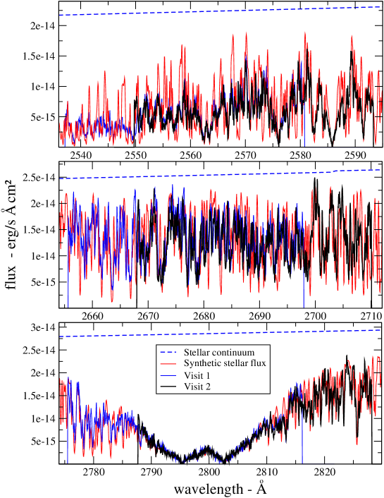
Figure 1: HST/COS NUV spectra of WASP-12 (Visit 1: blue line; Visit 2: black line) and a scaled model WASP-12 stellar spectrum (red line). The stellar continuum (dashed blue line) lies well above the observed flux due to overlapping stellar absorption features throughout the spectrum. The mean flux is slightly lower in Visit 2; see text. The three panels show the NUVA, NUVB, and NUVC spectral regions.

Figure 1 shows the flux-calibrated grand sum spectra obtained in Visit 1 and Visit 2 in comparison with synthetic fluxes, as discussed in §3.2. The mean fluxes are $9\pm 1$%, $7\pm 1$% and $3.5\pm 1.0$% lower in Visit 2 for NUVA, NUVB, and NUVC respectively. This is largely attributable to the declining throughput (Osten et al 2010), but also due to the varying mean obscuration of the WASP-12 stellar flux by the planet and diffuse gas. We will discuss a likely third contributor to varying fluxes in §3.6.

In our time-series analysis we used the count rates obtained after background subtraction, rather than the flux calibrated spectra. The high quality flat-field and the relatively low background of the NUV channel mean the uncertainties are dominated by Poisson statistics. The resulting signal to noise ratio (SNR) in our extracted NUVB spectra is $\sim$8 per pixel for each 3000 sec exposure. This is consistent with the expected photon counting noise, and propagates to a fractional uncertainty of $\sim 0.007$ when a 3000 s exposure is averaged.

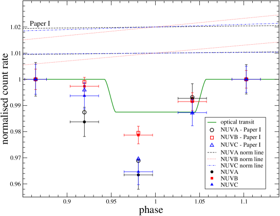
Figure 2: The Visit 1 results from Paper 1 (open symbols) compared to the same data re-reduced with the updated calibration files (closed symbols). The normalisation lines indicate the tilt which has been removed from the data in setting the first and last point to unity (i.e. the first two points in the NUVB light curve were moved slightly upwards). The upper set of normalisation lines correspond to the Paper 1 reduction. The green line shows the model transit of the optically opaque planet across a uniform brightness stellar disc.

Figure 2 shows our Visit 1 light curves. These were produced by summing across wavelength for each of NUVA, NUVB and NUVC to produce a photometric point for each HST orbit. Fig. 2 compares the results from Paper 1 with those from our revised calibration. The first and last data points for both reductions are set to unity with the normalisation procedure applied in Paper 1; all the remaining points are within 1$\sigma$ of their previous positions. For all three wavelength regions, the normalisation lines (see Paper 1) are slightly improved (flatter) with the new calibration files. The normalisation applied does not significantly affect the shape of the observed NUV transit, as no point moves by as much as 1$\sigma$.

The NUVA point immediately preceding optical ingress and the NUVA and NUVC points at mid-transit have been moved down almost $1\sigma$ relative to the reduction presented in Paper 1. The refined reduction therefore strengthens the case (made in Paper 1) for an early ingress and an extended asymmetric cloud of absorbing gas: the NUVA and NUVC transit depths are now $\sim 4\sigma$ below the depth of the optical transit. When we consider the data from both visits together, however, these conclusions become more complicated, as discussed in §3.3.

2.2 PIRATE optical photometry

Table 2: WASP-12 observations with PIRATE.

Date	HJD start	HJD end	Exp.	Comments
(BON)	-2455000	-2455000	Time (s)
15/10/2009	121.53078	121.68142	120s	OOT only
18/10/2009	123.49117	123.67301	120s	OOT only
11/11/2009	147.47507	147.62549	120s	Egress & OOT.
				High humidity ($>$ 90%)
12/11/2009	148.47187	148.51421	60s	OOT & ingress
22/11/2009	158.37221	158.69467	60s	Egress & OOT
23/11/2009	159.44126	159.59863	60s	Mid-transit, egress & OOT
13/01/2011	575.26270	575.36230	45s	Used PIRATE Mk. 2
				Holmes et al. (2011)

In conjunction with our first HST visit we undertook a program of optical photometry with The Open University’s remotely operable optical telescope, PIRATE (Holmes et al. 2011). The goal of these observations was to verify or, if necessary, update the WASP-12 b orbital ephemeris. The PIRATE observations are logged in Table 2. We used the R filter on all 7 nights, and either 120s, 60s, or 45s exposures. The dead time between exposures is 15s, resulting in a cadence of 135s, 75s, or 60s. We captured one ingress, four egresses, and on two nights OOT coverage only. The control computer’s real-time clock was synchronized every hour with a USNO time server, typically requiring 11-13s correction each time. Light curve precision was 2.5-2.8 mmag, which we achieved through an iterative comparison-ensemble procedure (Holmes et al. 2011). The light curve of one egress is published in Holmes et al. (2011, their Fig. 7), and we present our phase-folded optical light curve in Sect. 3.1 below.

2.3 Faulkes Telescope North optical photometry

The Spectral camera on the 2m Faulkes Telescope North, Hawai’i, was used to observe WASP-12 on 2010 December 17 UT through a Bessell-B filter. The Spectral camera is a 4096x4096 pixel Fairchild CCD486 BI which was used in bin 2x2 mode giving a 0.304 arcsec/pixel scale over the $10\times 10$ arcmin field of view. We used a 22 s exposure time, which gave a cadence of about 47 s. The start and end time of the observations were HJD_UTC 2455547.913994473 and 2455548.085096728 respectively. The timeseries data were preprocessed using the standard ARI pipeline and aperture photometry was performed using IRAF/DAOphot.

2.4 James Gregory Telescope photometry

A partial transit was obtained in photometric conditions on 30 November 2008 with a 1k $\times$ 1k CCD detector mounted on the James Gregory Telescope (JGT), a $0.95$ m Schmidt-Cassegrain telescope at the University of St Andrews. The full field of view (FOV) of the detector is $17^{\prime}$ with a 1 arcsec/pixel platescale, however vignetting and aberrations create an effective FOV for photometry of approximately $10^{\prime}$. Cousins-R band exposures of 90s duration were taken over 3 hours from HJD_UTC = 2454801.388296 to 2454801.517059, with a total of 104 photometric points. Standard image processing, source detection and aperture photometry were performed using the Cambridge Astronomical Survey Unit catalogue extraction software (Irwin & Lewis 2001). The software has been compared with SExtractor and found to be very similar in the completeness, astrometry and photometry tests. We adopted an 8 pixel radius aperture to match the typical seeing for the night (FWHM $\sim 8^{\prime\prime}$). Differential photometry was generated from the instrumental magnitudes using the combined flux of 7 nearby stars of similar brightness to WASP-12.

3 Results and Interpretation

3.1 The Orbital Ephemeris

The elapsed time between the WASP-12 b discovery paper photometry (Hebb et al. 2009) and our two HST visits was 18 months and two years respectively. Since we anticipated the interpretation of our NUV time-series data could be critically dependent on the WASP-12 orbital ephemeris, we re-examined it. We took our PIRATE, FTN and JGT data, the Liverpool Telescope Z band from Hebb et al. (2009), together with all available SuperWASP data, and determined a new linear ephemeris using the MCMC fitting routine of Collier Cameron et al. (2007), updated by Enoch et al. (2010), as used by the SuperWASP consortium. We obtained a new ephemeris of

$$T_{\rm mid}({\rm HJD})=2454852.7739^{+0.00014}_{-0.00014}+N\times 1.09142206^{+0.00000033}_{-0.00000031}$$ (1)

Excluding the SuperWASP data and those observations that did not capture any part of the transit, we then examined the data for transit timing variations (TTVs). We phase-folded the 15 remaining light curves, and renormalised each observation against a model light-curve appropriate to its color using $\chi^{2}$ minimisation. A phase offset from Eqn. 1 was determined by $\chi^{2}$ minimisation for each individual light curve. These offsets define the observed (‘O’) mid-transit time for each observation and the deviations (‘O-C’) from the mid-transit time calculated from Eqn. 1 (‘C’) are tabulated in Table 3.

Table 3: Transit mid-times

$T_{\rm mid}$ (‘O’)	$\sigma(T_{\rm mid})$	‘O-C’	Source
(HJD- 2450000)	(s)	(s)
4515.52455	11.32	5.65793	LT (Z)
4801.47593	35.83	-98.07082	JGT (R)
5123.44587	60.35	-60.35127	PIRATE (R)
5147.45781	77.33	-3.77195	PIRATE (R)
5148.55083	113.16	133.90439	PIRATE (R)
5158.37107	49.04	-86.75496	PIRATE (R)
5159.46575	52.81	194.25566	PIRATE (R)
5548.00980	20.75	3.77195	FTN (B)
5575.29570	54.69	33.94759	PIRATE (R)

Our linear ephemeris is well constrained at either end by precise measurements from Liverpool Telescope and the Faulkes Telescope North. Maciejewski et al (2011) observed two transits and suggested their measurements might constitute TTV detections. We note that our new ephemeris is consistent with the Chan et al (2011) transit timings and that we suspect the error estimates of Maciejewski et al (2011) are rather optimistic. Other light curves gathered with comparable facilities lead to larger timing uncertainties.

None of the PIRATE or JGT observations captured complete transits, which is one reason why they have large timing uncertainties. We would not claim a detection of TTVs/TDVs based on these data alone. WASP-12 b may exhibit TTVs with amplitudes of $\sim 200$ s. Further high quality light curves are needed to address this hypothesis.

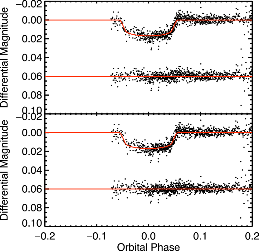
Figure 3: PIRATE R band data folded about our linear ephemeris (Eqn. 1); the residuals after subtracting the R band model from the SuperWASP MCMC run (red line) are shown offset. Top panel: with phase-offsets corresponding to the O-C values applied to the data. Bottom panel: without the phase-offsets applied.

3.2 NUV Spectroscopic coverage

Figure 1 shows the grand total flux calibrated spectra for our two HST visits. The Visit 2 spectral coverage is redwards of the Visit 1 coverage, and the two ranges overlap for about half of the total coverage. As noted in §2.1 the Visit 2 spectra have slightly lower fluxes, largely due to the (uncalibrated) decline in COS throughput. Both spectra are RV-corrected to the WASP-12 rest frame by line profile fitting to the two spectra, thus determining an empirical wavelength offset between the two visits. This correction was applied before generating Figure 1 and subsequent figures.

Figure 1 also shows the stellar continuum level (dashed line). There is prodigious stellar photospheric absorption in WASP-12’s atmosphere throughout; no point in our NUV spectra is consistent with unabsorbed continuum. Figure 1 shows synthetic fluxes calculated using the LLmodels stellar model atmosphere code (Shulyak et al. 2004), assuming the fundamental parameters, metallicity and detailed abundance pattern given by Fossati et al. (2010b). LLmodels assumes Local Thermodynamical Equilibrium (LTE) for all calculations, adopts a plane-parallel geometry, and uses direct sampling of the line opacity allowing the computation of model atmospheres with individualised (not scaled to solar) abundance patterns. We used the VALD database (Piskunov et al. 1995; Kupka et al. 1999; Ryabchikova et al. 1999) for the atomic line parameters. The resolution applied to the synthetic fluxes matches that of COS, but we did not model the peculiar line spread function (LSF) of HST. The differences between the synthetic and observed spectra are predominantly caused by the HST LSF.

All three regions are affected throughout by many blended photospheric absorption lines. We observe no unabsorbed stellar continuum. The NUVA region is strongly absorbed by many overlapping lines, with lines of MgI and FeI predominating; the NUVB region for both visits is closest to the continuum; while the NUVC region is dominated by absorption in the broad wings of the strong Mg II doublet at 2795.5 Å and 2802.7 Å.

3.3 NUV Transit Light Curve

Table 4: Simple transit model fits to NUV light curves. The free parameters are the phase offset from the optical ephemeris, $\Delta\phi$, and the radius, $R$, of a circular occulting disc, expressed as a fraction of the stellar radius. We constrained our search to $R/R_{*}\geq 0.1119=R_{\rm P}/R_{*}$.

BAND	VISIT(S)	$\chi^{2}_{\nu}$	$N_{params}-$	$R/R_{*}$	$\Delta\phi$
			$N_{data}$
A	1	0.276	2	0.189	-0.0279
B	1	0.864	2	0.146	-0.0186
C	1	0.276	2	0.186	-0.0170
A	2	7.77	2	0.118	-0.124
B	2	4.11	2	0.113	0.0050
C	2	8.32	2	0.136	-0.1271
A	2NF	11.5	1	0.237	-0.0475
B	2NF	8.22	1	0.116	-0.0204
C	2NF	15.8	1	0.224	-0.0499
AO	1,2	4.002	6	0.147	-0.0241
BO	1,2	1.823	6	0.129	0.0034
CO	1,2	4.74	6	0.122	0.0198
AO	1,2NF	4.38	5	0.1633	-0.0268
BO	1,2NF	1.25	5	0.1415	-0.0159
CO	1,2NF	3.53	5	0.1424	-0.0368

In Paper 1 we observed an NUV transit which was significantly deeper than the optical transit, and which began with an early ingress compared to the optical ephemeris. These conclusions from our Visit 1 data alone are strengthened by the re-reduction described in §2.1. We quantify this by fitting the simplest possible transit model, assuming a circular occulting disc transiting a uniform brightness (no limb-darkening) star. We fix all the parameters of this model to the values demanded by WASP-12 b’s optical transit except for two free parameters: $R/R_{*}\geq R_{\rm P}/R_{*}$, and $\Delta\phi$, describing the radius and phase offset of the NUV occulting disc compared to the transit of the optically opaque planet with $R=R_{\rm P}$ and $\Delta\phi=0$ across the star of radius $R_{*}$. The normalisation of the data to the model is also a free parameter. We report our model fitting in Table 4, using the reduced-$\chi^{2}$ statistic, $\chi^{2}_{\nu}$, which is the appropriate statistic for assessing the goodness of fit. For completeness we also report the number of degrees of freedom, i.e. the number of parameters including normalisation, minus the number of fitted data points. The results for Visit 1 shown in Fig. 4 and at the top of Fig. 5 and Table 4 are consistent with Paper 1: for NUVA, NUVB, and NUVC the best-fit transits are early by 43 min, 29 min, and 26 min respectively. As Table 4 shows, the best-fit radii for the occulting disc are significantly enhanced compared to that of the optically opaque planet ($R_{\rm P}/R_{*}=0.1119$, Chan et al 2011) with an enhancement in radius of $70\%$, i.e. almost a factor of three in area, for the NUVA and NUVC bands. The NUVA and NUVC bands provide extremely sensitive probes for the presence of low density gas at temperatures of several thousand degrees because these bands contain $\sim 10^{3}$ overlapping spectral lines. We discuss the spectral information in detail in §3.4 below. We do not imagine that the low density gas we have detected surrounding and preceding WASP-12 b actually presents a circular cross-section to us during its transit; this was the simplest model we could imagine, and we have few data points to fit. As the upper panels in Fig. 5 show, with two free parameters (three including normalisation) the model is already able to produce an improbably good fit to the data, and this suggests that our error bars (derived from photon-counting statistics) are not under-estimated.

Figure 4: $\chi_{\nu}^{2}$ grids from fitting model transits to our Visit 1 NUV data. We model circular opaque discs transiting a uniform brightness stellar disc. By allowing the normalisation of the model light curves to vary we find the best-fit transit for each value of phase and radius ratio without making any assumptions about which of the empirical points represent out of transit coverage. All three light curves are best fit by transits which occur early, and the best fit models in all cases correspond to discs much larger than that of the optical planet: $R_{\rm P}/R_{*}=0.1119$, which is the smallest value of $R/R_{*}$ shown.

Figure 5: The best-fitting simple transit models (solid lines) for each of our NUV light curves (diamonds). Triangles show the integral of the best-fit model over the exposure times used. In Visit 1 we obtain good fits which reveal an NUV transit deeper than the optical transit, and an early ingress. Visit 2 is less clear-cut: the 3rd data point in all three bands is high compared to the models fitting Visit 1, particularly for NUVA and NUVC. For these two bands the best fit model places this anomalously high point after egress so the ‘best-fit’ transit does not overlap the optical transit (dotted line).

Visit 2 was timed to provide coverage of the orbital phases missing due to Earth-occultation in our Visit 1 data. The two visits provide well-sampled coverage between $-0.17<\phi_{\rm orb}<0.12$. Unfortunately the Visit 2 data defy straightforward interpretation. The lower panels of Fig. 5 show the Visit 2 data along with the best-fit simple transit models to the three NUV bands. As the corresponding entries in Table 4 show, none of these fits are formally acceptable, with $\chi^{2}_{\nu}$ significantly above 1 in all cases. The NUVB band produces the best fit transit for Visit 2, but this fit essentially reproduces the transit of the optically opaque planet (dotted line in Fig. 5), with points before and after the transit deviating significantly from the model. The best-fit NUVB model is slightly late compared to the optical transit because the Visit 2 point which samples optical ingress is higher than the optical transit would predict. The Visit 2 NUVA and NUVC light curves strongly resemble each other. Throughout, the point-to-point deviations in the two light curves appear similar. In both cases the Visit 2 data is strongly absorbed before optical first contact, with the point sampling optical ingress lying above the out of transit level, while the Visit 1 data appears more strongly absorbed between optical second and third contacts. The best-fitting model for the Visit 2 NUVA and NUVC light curves is a transit which occurs so early that it fails to overlap the optical transit. This is clearly unphysical: the planet is surely opaque to NUV light. These fits result from the anomalously high third data point (arising from the third HST orbit) in the Visit 2 NUVA and NUVC light curves: in both cases the exposure spanning the optical ingress is the 2nd-highest in the light curve. Our simple model requires a strict relationship between the depth and duration of the fitted transit. Since the ‘orbit 3 point’ is high, the model places it above the out-of-transit level and as the pre-optical-ingress NUVA and NUVC data points are both lower than the fitted out of transit level, the best-fit transit model places the entire transit early.

The aberrantly high Visit 2 orbit 3 data point in the NUVA and NUVC light curves thus defies the simple explanation we developed from Visit 1. We can think of three plausible explanations for this: (i) these are noisy data and this simply happens to be a point with a positive deviation; (ii) there was a short-lived stellar flare during Visit 2 orbit 3; (iii) the gas which absorbs before first contact is clumpy, and there was a clear window to the star during Visit 2 orbit 3. Vidotto, Jardine & Helling (2011)’s bow shock model can produce such a ‘window’ configuration. The same pattern independently appearing in both the NUVA and NUVC light curves makes the first explanation far less likely than it would otherwise be, and our fits to the Visit 1 light curve suggest our error estimations are ample. We will discuss the stellar flare hypothesis in §§3.6 and  4.1, and the window hypothesis in §4.1.

Figure 6: The fits which result for Visit 2 if we mask out the aberrant third data point. The NUVA and NUVC fits have absurd depths because the observed transit has a long duration and we fit a circular occulter. A more plausible model would have absorbing gas extended in the orbital plane. Symbols as in Fig. 5.

The Visit 2 data with the aberrant 3rd-orbit data masked out produces the fits shown in Fig 6 and Table 4 (entries for visit ‘2NF’). The NUVB fit now has a slightly deeper transit which occurs earlier because the fit has placed the orbit 4 point to span the beginning of egress. This fit, and the adjustments to it we might make if we relax our arbitrary assumption that the extended gas presents a circular cross-section, is consistent with the interpretation we made in Paper 1. The NUVA and NUVC ‘best’ fits are comical. Because the orbit 1, 2, and 4 points in both cases lie so far below the orbit 5 point, the relationship between transit depth and duration favors fits in which the transit depth is much deeper than any data point. A more sensible interpretation would be that the absorbing gas is extended along the orbital plane and presents a significantly non-circular cross-section, so the duration is longer than that of the models while the depth is shallower.

The fits we have performed separately on the two individual visits suggest that the configuration of the absorbing gas changed between the two visits. Indeed Vidotto, Jardine & Helling (2011) interpret this variability. Nonetheless for completeness we now proceed to examine the data from the two visits together.

Fig. 7 interleaves the two visits using only the photons detected within the overlapping wavelength regions of the RV-corrected spectra. It is immediately apparent that the Visit 1 data (black circles) lies above the Visit 2 data (red triangles). We attribute this to the known declining throughput of the COS/G285M configuration (Osten et al 2011). We corrected for this by boosting the Visit 2 count-rates by 5.52% using an estimate from Osten et al (2010), but the rate of sensitivity decline is not precisely known for our instrument configurations. The ‘corrected’ Visit 2 data are shown as blue squares.

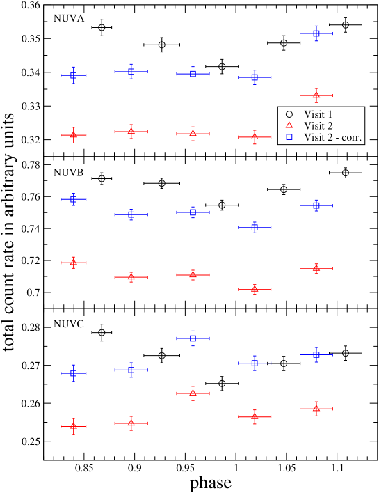
Figure 7: Count rates from the NUVA, NUVB, and NUVC overlapping spectral regions in the two HST visits. Circles show Visit 1, triangles show Visit 2, and squares show Visit 2 after multiplying by 1.052 to correct for the decline in instrument sensitivity between the two visits.

The background level differed between the two visits, with roughly twice as many background counts during Visit 2. The temporal behaviour of the background also differed, with a gradual increase in background during Visit 1 contrasting with a decrease in background during Visit 2. We corrected for background, so this should not affect our light curves. The corrected Visit 2 data appear to match well at phases following the transit for NUVA and NUVC, but the corrected NUVB light curve from Visit 2 appears systematically lower than the Visit 1 light curve. The Visit 2 orbit 3 point remains aberrant in NUVC, but restricting the wavelength coverage to only the overlapping region has dramatically lowered the NUVA orbit 3 point. We will return to discuss the reasons for this in §4.1.

Our NUV light curves, particularly the NUVA and NUVC bands, suggest that in Visit 2 perhaps the absorbing gas obscured the stellar disc at phases as early as $\phi_{\rm orb}=0.83$, in which case Visit 2 contains no genuine pre-transit data. Fig. 8 shows the light curves produced using all the data (i.e. not just the overlapping wavelength regions), arbitrarily setting the last point in each visit to (an out-of-transit level of) 1.0. The NUVB light curve now looks perfectly consistent with the interpretation we made in Paper 1: the transit is deeper than the optical transit and appears to be preceded by absorption occurring before optical ingress. The NUVA and NUVC light curves also look reasonably consistent with this interpretation, with much more significant pre-ingress absorption occurring in Visit 2.

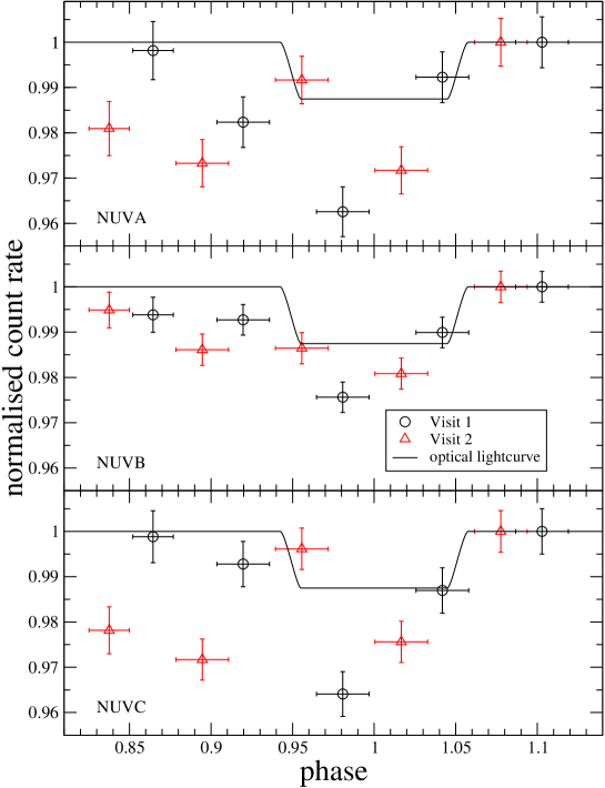
Figure 8: The light curves from all of our HST data, with each HST visit normalised to unity in the last HST orbit. Note the wavelength regions contributing to the two visits differ, as indicated in Figure 1.

We performed simple transit fits (as described above) to the combined data from the overlapping wavelength regions in the two visits, allowing the normalisation of each visit to vary independently. These fits thus have four free parameters in total: $R$, $\Delta\phi$, and two independent normalisation values. Fig 9 shows the best fitting models, along with the data after applying the best fit normalisations. As Table 4 quantifies (entries for bands AO, BO, CO; Visits ‘1,2’), none of the three fits in Fig. 9 are formally acceptable. Nonetheless, the NUVA and NUVB fits are broadly consistent with our interpretation in Paper 1. The best-fit transit is significantly deeper than the optical transit and the light curves show signs of absorption from diffuse gas before optical ingress. The NUVC band produces formally the worst fit, and the first half of the light curve shows enormous scatter between the sets of points from the two visits. The best fit model transit is late compared to the optical transit: a fit which moved the ingress to after the anomalously high Visit 2 orbit 3 point has been preferred.

Figure 9: The best-fitting simple transit models for our interleaved NUV data. None of the fits are formally acceptable, but the NUVA and NUVB results are broadly consistent with a deeper transit than the optical and absorption from diffuse gas which precedes the optical transit (dotted line). The best-fit NUVC transit occurs late, but the first half of the interleaved lightcurve has extremely high scatter so this fit should clearly not be taken at face value. Symbols as in Fig. 5.

Figure 10: The best-fitting simple transit models for our interleaved NUV data with the Visit 2 Orbit 3 point masked out. None of the fits are formally acceptable, but the results are broadly consistent with a deeper transit than the optical and absorption from gas preceding optical transit (dotted line). Symbols as in Fig. 5.

Figure 10 shows the best fits to the interleaved data without the Visit 2 orbit 3 point. These fits (entries for Visits ‘1,2NF’) are all broadly consistent with our Paper 1 conclusions. For the NUVB and NUVC bands, the best $\chi^{2}_{\nu}$ is better than the fits shown in Fig. 9.

In both NUVA and NUVC, as Figure 1 shows, the wavelength ranges covered only by the Visit 1 data are strongly absorbed by the stellar photosphere, while the wavelength ranges covered only by the Visit 2 data are significantly less strongly absorbed. If the diffuse absorbing gas has broadly the same ionic composition (i.e. abundance mix and temperature) as the stellar photosphere, this would predict a deeper transit in Visit 1 NUVA and NUVC than in Visit 2 NUVA and NUVC. This is exactly what Fig. 5 and Table 4 show.

Figure 1 shows that the NUVB spectral region, for both visits, is the closest to the stellar continuum: there is relatively little photospheric absorption, and we might similarly expect relatively little absorption from the extended cloud of diffuse gas. Of course, without knowing the composition and physical conditions of this gas, it is impossible to assert this is definitely true, but it is the simplest assumption one could make a priori. Our NUVB data suggests a deeper transit than that of the optical light curve, but of the three spectral regions it is the closest to the optical curve. Note the NUVB data have the smallest uncertainties because, being relatively unabsorbed, we detect most photons from the star in NUVB.

Each (version of the) NUVB light curve (Figs. 5,  6,  7,  8,  9 and  10) shows indications of an early ingress in NUVB. Our NUVA and NUVC light curves are also broadly consistent with this, except for the anomalous count rates observed in Visit 2 orbit 3. This aberrant point appears in both NUVA and NUVC when we considered the entire wavelength range (Figs. 5 and  8) but only in NUVC when we extract light curves from the overlapping wavelength ranges (Figs. 7 and  9). The Visit 2 orbit 3 NUVA point shifts downwards by $4\sigma$ when we restrict the wavelength range. We think this is significant and will return to discuss the implications of this piece of evidence in §4.1.

In summary, the NUV light curves are broadly consistent with our principal conclusions in Paper 1. The transit is deeper than in the optical, and is preceded by an early ingress, though the point for the third orbit in Visit 2 deviates from this description when some wavelength regions are considered. There is clearly NUV absorption occurring before optical first contact.

3.4 The wavelength resolved transit

The enhanced transit depths seen in Figs. 4, 5, 6, 8, 9 and 10 result from summing over the $\sim 40\AA$ covered in each of our NUVA, NUVB and NUVC spectra (or the $\sim 30\AA$ of overlapping wavelength coverage for the last two figures listed). The enhancement of the NUV transit depth compared to the optical transit depth is due to absorption in the diffuse gas surrounding the planet. This absorption is caused by bound-bound transitions in atomic and ionic species. A priori we do not know which species are present in this gas, but we do know that there are thousands of overlapping spectral lines within the wavelength ranges we have observed. Since we have time-series spectral data, we can examine the transit at any spectral resolution greater than or equal to that of the data. In Paper 1 we presented evidence for detections of enhanced transit depths in Mg II and other lines of neutral and ionised metals. With the addition of Visit 2 we have extended our wavelength coverage, our temporal coverage, and increased the SNR of the overlapping wavelength region, so we examined our Visit 1 and Visit 2 data afresh for evidence of enhanced transit depths at particular wavelengths.

Table 5: online material Wavelength of the Visit 1 and Visit 2 spectral points deviating more than 3$\sigma$, adopting two different $\sigma$s: $\sigma_{d_{\lambda}|_{exp}}$ and $\sigma_{d_{\lambda}|_{prop}}$. The deviating points highlighted in bold face are the Visit 2 points which are one resolution element away from a Visit 1 point. All wavelengths are given in Å.

Wavelength	Wavelength	Wavelength	Wavelength	Wavelength	Wavelength	Wavelength	Wavelength	Wavelength	Wavelength	Wavelength	Wavelength
$\lambda-2000$Å	$\lambda-2000$Å	$\lambda-2000$Å	$\lambda-2000$Å	$\lambda-2000$Å	$\lambda-2000$Å	$\lambda-2000$Å	$\lambda-2000$Å	$\lambda-2000$Å	$\lambda-2000$Å	$\lambda-2000$Å	$\lambda-2000$Å
Visit 1	Visit 2	Visit 1	Visit 2	Visit 1	Visit 2	Visit 1	Visit 2	Visit 1	Visit 2	Visit 1	Visit 2
3$\times\sigma_{d_{i}|_{exp}}$	3$\times\sigma_{d_{i}|_{exp}}$	3$\times\sigma_{d_{i}|_{prop}}$	3$\times\sigma_{d_{i}|_{prop}}$	3$\times\sigma_{d_{i}|_{exp}}$	3$\times\sigma_{d_{i}|_{exp}}$	3$\times\sigma_{d_{i}|_{prop}}$	3$\times\sigma_{d_{i}|_{prop}}$	3$\times\sigma_{d_{i}|_{exp}}$	3$\times\sigma_{d_{i}|_{exp}}$	3$\times\sigma_{d_{i}|_{prop}}$	3$\times\sigma_{d_{i}|_{prop}}$
NUVA				NUVB				NUVC
538.484		537.535		661.605		657.054			792.434	776.577
539.002		537.880		662.022		664.316		793.963		776.818
539.045		538.139		663.649		664.816		794.442		778.785
543.442		538.312		666.649		666.691		794.842		779.026
546.758		538.916			667.763	666.733		794.922		784.399
557.028		538.959			667.888		667.763	795.401		785.040
562.344		539.520		669.522			669.432	795.561			787.704
562.473		539.606		670.313			669.474	795.641			787.945
	563.215	540.166			671.851		672.310	797.957			788.065
563.501		540.641			672.018		678.558	801.428		788.524
	575.914	540.856			678.807		680.804	802.185			790.952
575.980		540.900		678.956		684.179		802.425		791.004
	575.999	541.072		682.895			686.995	802.504		791.084
576.151		541.158		682.978		687.491		803.023		791.164
	576.342	541.201		684.759			687.908	803.142			791.513
	576.385	541.891			689.360	690.056				791.604
	576.470	542.107			690.936	691.089					792.274
	577.883	542.193			690.978		692.470				792.314
580.925		542.537		695.261		692.618					792.674
	582.286	542.581			698.681		692.802			793.123
	585.873	543.873			698.805	694.601					793.235
	586.043	543.916			698.847	695.261				793.243
		544.347			706.904		695.370			793.403
		544.390			710.368		695.784			793.443
		544.433					697.233			793.483
		546.155					700.873				793.635
		546.198					703.146				793.715
		546.241					706.408			793.723
		546.715					710.080				793.755
		547.490					710.203			793.803
		547.705					710.327			793.843
		548.952					710.368			794.003
		549.425								794.083
			549.902								794.116
		549.984								794.402
		550.027									794.436
			550.248							794.522
			550.291								794.956
			550.550								794.996
			550.636								795.196
			550.680								795.276
		550.887									795.316
			551.629								795.356
			551.758								795.397
			551.802								795.477
			552.708							795.481
			553.010								795.517
			553.139							795.521
		553.465									795.597
			554.131							795.601
			554.691								795.637
			555.424							795.721
			555.510							795.920
			556.975							796.080
			557.277							796.120
			557.578							796.160
			558.310							796.200
			558.396							796.280
			558.870								796.357
		558.916								796.479
		559.173									796.557
			559.387								796.597
			559.430								796.637
			559.774							796.639
		559.816								796.679
		559.859									796.717
			560.075								796.797
			560.549								796.917
			561.237							796.919
			561.280								796.957
			561.796								797.197
			561.925							797.318
			562.312							797.358
		562.558								797.438
			562.570							797.478
		562.601								797.518
			562.871								797.717
			562.914							797.797
		563.372								797.837
			563.387							797.917
		563.415								797.997
			563.430								798.157
			563.516								798.517
			563.645								798.756
			563.731							798.875
			564.161							799.114
			564.548							799.633
			564.762								799.956
			565.063								800.355
			566.824								800.395
			566.996								800.475
		567.823									800.515
			568.026								800.675
		568.635									800.715
			569.314							800.790
			569.700								800.994
			569.828								801.434
			569.957							801.548
		570.857									801.634
		570.900								801.707
			571.115								801.754
		571.541								801.787
		571.712									801.873
			572.101								801.913
			572.873							801.986
		574.444									802.033
			574.544							802.146
			574.886								802.153
		575.212									802.233
			576.171							802.305
			576.299								802.353
		576.450								802.385
			576.642								802.432
			576.770							802.465
			576.813							802.544
		577.473								802.584
			577.540								802.592
		578.070								802.624
			578.096							802.704
		578.240								802.744
			578.310								802.872
		579.519									803.151
		579.732									803.391
			581.517								803.990
			584.251							804.059
			584.550								804.349
			585.190							804.975
			585.275							805.015
			585.361								805.187
			585.659							805.254
			585.915							805.334
			586.299							805.453
			586.342								805.785
			586.427							806.091
			586.897							806.569
			587.963							806.688
			588.432								806.743
			592.309								806.783
											806.942
											807.102
											807.261
										807.524
											807.580
											807.700
											807.860
										809.116
											810.052
										810.111
											811.008
											811.367
										811.861
											814.034
										814.444
										816.192
										816.232
											816.421
											817.455
											817.813
											819.363
											820.833
											822.978
											828.253
											828.293

Table 5: continued.

We used the methods of Paper 1 to detect wavelengths with significantly over-deep transits. In Paper 1, we used the average of orbits 1 and 5 for the out of transit (OOT) spectrum, and orbit 3 for the in transit (IN) spectrum. As Fig. 2 and Fig. 5 demonstrates, there is no reason to change this, so we used the same portions of data (re-reduced as detailed in Section 2.1). Visit 2 shows no clear pre-ingress OOT data, so in this case we used orbit 5 for the OOT spectrum, and orbit 4 for the IN spectrum. Consequently the propagated error estimate for our Visit 2 OOT spectrum is larger that that for the Visit 1 OOT spectrum.

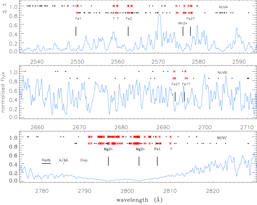
Figure 11: The wavelengths at which significantly over-deep transits were detected are indicated with a black cross, except for those wavelengths detected in both visits where we use a large red asterix instead. The upper row and lower rows of symbols correspond to Visit 1 and Visit 2 respectively. The horizontal scale bars in the bottom (NUVC) panel indicate the spectral dispersion, the spectral resolution, and the magnitude of WASP-12 b’s orbital velocity. The blue line is the synthetic stellar spectrum, normalised to the continuum level, with a resolution of $R=10,000$, adopted to simulate the HST LSF. We do not use the synthetic stellar spectrum in our analysis. Wavelengths of a few absorbing species are identified, with a small asterix after the ion identification for resonance lines.

For each visit, we define the ratio spectrum, $d_{i}$ (= IN / OOT ), where IN is the in-transit flux and OOT is the out of transit flux, to measure the transit depth at wavelength $\lambda_{i}$. We examine $d_{i}$ to determine wavelengths $\lambda_{i}$ with statistically significant excess transit depths. These are the wavelengths where the diffuse gas absorbs. These individual contributions combine to produce the excess depth in the light curves examined in §3.3. We report the wavelengths of these points in Table LABEL:tab:lam_id and in Fig. 11. In Table LABEL:tab:lam_id we use two different criteria to assess anomalously low points, i.e. those deviating by 3$\sigma$, as we did in Paper 1. The first of these examines the ratio spectrum against the error estimate we obtain from the propagated (Poisson-dominated) errors in the reduction. We label this error estimate as $\sigma{d_{i}|_{prop}}$, and report in Table LABEL:tab:lam_id wavelengths where the ratio spectrum is 3$\sigma{d_{i}|_{prop}}$ or more below the median value of the ratio. These wavelengths are also indicated in Fig. 11. The second assessment uses the RMS scatter, $\sigma_{d_{i}|_{exp}}$, within the ratio spectrum itself in the criterion. As Fig. 3 of Paper 1 showed, the $\sigma_{d_{i}|_{exp}}$ criterion is more likely to pick out points where the signal in the observed stellar spectrum is low.

Our ratio spectra have a total of just under 3100 points, so if the noise is Gaussian-distributed we expect $\sim 9$ distinct points in each to deviate by more than 3$\sigma{d_{i}|_{prop}}$. As Table LABEL:tab:lam_id shows, we find many more deviating points than this. In every case the points which deviate by more than 3$\sigma{d_{i}|_{prop}}$ are deviations below the median of the ratio spectrum, indicating extra absorption compared to the median. Where there are positive deviations, these are accompanied by large values of $\sigma{d_{i}|_{prop}}$ due to the low flux, and hence low SNR of the WASP-12 spectrum at that wavelength. Consequently, none of these positive deviations are 3$\sigma{d_{i}|_{prop}}$. We would expect, nonetheless, to find a small number ($\sim 4\pm 2$) of positive deviations due to white noise, but we do not. Possibly our propagated errors are slightly over-estimated. This leads us to conclude we have detected statistically significant excess absorption at $\sim 200$ distinct wavelengths in each visit from the gas around WASP-12.

As noted in §3.3 the NUVA and NUVC spectral regions are more strongly absorbed within the stellar photosphere than is NUVB. In §3.3 we showed that the transit is deeper in wavelength regions where the photospheric absorption is strong. These wavelength regions contain overlapping spectral lines which produce strong photospheric absorption of the underlying stellar continuum. To the extent that the extended diffuse gas cloud has similar abundances and temperature as the stellar photosphere, it too will produce strong absorption in these wavelength regions. Fig. 11 supports this: it is immediately obvious that there are far more wavelengths exhibiting enhanced transit depths in NUVA and NUVC than there are in NUVB. It is also clear that the wavelengths exhibiting excess transit depths generally occur where the emergent stellar flux is low. This shows our rule of thumb works well: the photospheric absorption within a wavelength range is a good predictor of the likely diffuse absorption.

Fig. 11 shows that our identified wavelengths in NUVC from the two distinct visits are largely associated with absorption in the wings of the Mg II resonance lines. This is clearly and unambiguously detected in both visits, and at so many distinct wavelength-pixels that the median value of the ratio spectrum must be lowered by them. Away from the cores of Mg II at $\sim 2788-2789\AA$, $\sim 2811-2812\AA$ and $\sim 2815\AA$ there is a suggestion of a consistent wavelength shift between the Visit 2 (upper) and Visit 1 (lower) detections, with the Visit 1 transits being redshifted by $\sim 0.5-1\AA$ ($\sim$ 50-100 $\mathrm{km\,s}^{-1}$). This shift is much greater than our spectral resolution, but less than the magnitude of the planet’s orbital velocity (230   $\mathrm{km\,s}^{-1}$), which is the natural velocity scale for motions of material orbiting the star. The NUVA and NUVB identified wavelengths show less consistency between the two visits, except for wavelengths consistent with resonance lines which are picked out in both visits.

The next step is to attempt to identify the spectral lines causing these enhanced transit depths. In Paper I we arbitrarily restricted our line identifications to resonance lines, and the consistently detected wavelengths in Fig. 11 show this was a sensible first step. Nonetheless, strong non-resonance lines of abundant elements may be more prominent than the resonance lines of rare elements. We attempted to assess this with a procedure which accounts for the stellar abundances derived for WASP-12 (Fossati et al. 2010b); the velocity shift required to match the rest wavelength of the line to the observed deviation; the excitation potential of the line; and the ${gf}$ value of the line. We introduce three simple functions: $P_{a}$, $P_{\Delta\lambda}$, and $P_{\chi}$, (each defined below) to estimate the effects of the first three of these factors on the likelihood of a particular identification being correct.

We wish to estimate the probability that an observed 3$\sigma$ deviation at wavelength $\lambda$, arises from absorption by spectral line $i$ of element $el$ which has rest wavelength $\lambda_{i}$. We consider a wavelength range $\lambda_{i}\pm\Delta\lambda$ and adopt $\Delta\lambda=$ 3 Å in our analysis to recover the full range of deviating points we identified in the broad wings of the Mg II lines in Paper 1 (see Fig. 3 therein.) This corresponds to a velocity shift slightly greater than the magnitude of the orbital velocity of WASP-12 b, but our procedure favours the smallest possible value of wavelength/velocity shift.

The wavelength shift required to match the observed point to rest wavelength is accounted for in the factor $P_{\Delta\lambda}$; the excitation potential, $\chi_{i}$, of the lower level in the factor $P_{\chi}$; and the abundance in the factor $P_{a}$. We define these probability factors by

$$P_{\Delta\lambda}=1-{\left({{|\lambda_{i}-\lambda|}\over{\Delta\lambda}}\right)};\quad~{}~{}~{}~{}~{}~{}~{}P_{\chi}=e^{-\frac{\chi_{i}}{kT}}\quad~{}~{}~{}~{}~{}P_{a}=\frac{N_{el}}{Z}$$ (2)

where $N_{el}$ is the abundance of the element considered, and $Z$ is the ‘metal’ abundance. Each gives a value of unity for the most favorable value of the quantity concerned; $P_{a}$ is unity if the proposed gas composition comprises only H, He and the element under consideration. $P_{\Delta\lambda}$ was designed to have a weak dependence on the shift $|\lambda_{i}-\lambda|$ as we expect the gas to have non-zero velocity w.r.t. the stellar rest-frame. $P_{\chi}$ is proportional to the expected population in the lower level, and $P_{a}$ is proportional to the number of absorbing atoms/ions.

$P_{\Delta\lambda}$, $P_{\chi}$ and $P_{a}$ are multiplied together and further multiplied by the ${\it gf}$ value of the line under consideration to give our estimated overall probability measure, $P_{i}$, that the deviation is associated with the specified spectral line, $i$. P_i in Eq.3 is thus not normalised to 1.

$$P_{i}=(P_{\Delta\lambda}P_{\chi}P_{a})\cdot({\it gf})_{i}$$ (3)

We then use this framework to assess the likely contribution to the measured deviation of all known spectral lines within $\Delta\lambda$. $P_{i}$ estimates the likely relative contribution of each of these lines to the detected absorption; summing over all lines estimates the total absorbing capacity, $P_{\rm tot}$. The fraction of this due to any given spectral line is our proxy for the likelihood, $L_{i}$ that this is the correct line identification.

$$P_{\rm tot}=\sum_{i}P_{i};\quad L_{i}=\frac{P_{i}}{P_{\rm Tot}}$$ (4)

This framework indicates, with some physical justification for our estimates, how the likely line identification depends on the assumed temperature and abundance pattern. Our factor to account for a decreasing likelyhood as the shift from the line’s rest wavelength increases is arbitrary, but adequate, given the complex COS LSF, the unknown velocity distribution in the absorbing gas, and the SNR of our data. The temperature dependence is only indicative: we have not used the Saha equation to determine the ionic balance. Figure 12 shows examples of applying this procedure to a selection of four points detected as having enhanced transit depths at significance of $3\sigma$ or more in Visit 1. Similarly Figure 13 shows a selection of line ID assessments from the Visit 2 data.

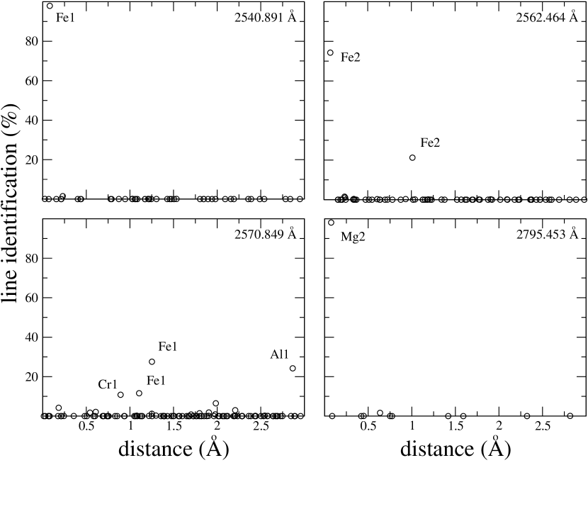
Figure 12: Line identifications from the Visit 1 data. The adopted temperature was 3000 K and an abundance pattern consistent with Fossati et al. (2010b) was assumed. The examples show three fairly firm identifications and one point where no firm conclusion is possible. $L_{i}$ is shown for every spectral line where it exceeded a value of $10^{-5}$, many lines considered had values of $L_{i}$ below this threshold.

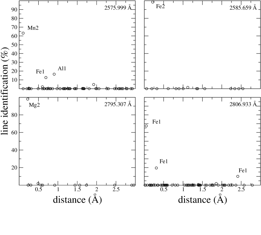
Figure 13: Line identifications from the Visit 2 data. The adopted temperature was 3000 K and an abundance pattern consistent with Fossati et al. (2010b) was assumed. The examples show three fairly firm identifications and one (top left) probable identification. $L_{i}$ is shown for every spectral line where it exceeded a value of $10^{-5}$, many lines considered had values of $L_{i}$ below this threshold.

In Fig. 12 the two upper panels reveal absorption from Fe I and Fe II causing enhanced transit depths at 2540.891 $\AA$ and 2562.464 $\AA$. The lower right panel shows the overwhelming probability that the enhanced transit depth at 2795.453 $\AA$ is caused by Mg II. This is because the imputed line is one of the pair of resonance lines with large ${\it gf}$ values which dominate the NUVC spectral region. For this line the $P_{\chi}$ and ${\it gf}$ factors are so large that the assumed Mg II abundance would need to be vanishingly small to identify any other nearby spectral line as likely to contribute significantly to the total absorption. Our Paper 1 detection of absorption in Mg II during Visit 1 remains unassailable under this more careful scrutiny. Visit 2 provides independent data, and as the lower left hand panel of Fig. 13 demonstrates, it shows the Visit 2 detection of an enhanced transit depth at 2795.307 $\AA$ can be confidently attributed to Mg II. Note the wavelength solutions produced by the simultaneous arc lamp spectra differ for the two visits, so we cannot compare pixels with identical wavelength sampling without rebinning. Rebinning is undesirable because adjacent pixels are then no longer independent.

Not all deviating points could be unambiguously associated with absorption by a single ionic species: the lower left panel of Fig. 12 and the upper left panel of Fig. 13 show examples where there are plausibly large contributions from a number of different elements. The detected absorption is likely to be a mix of the various spectral lines, with the dominant contributor(s) depending on the the unknown composition and physical conditions of the gas. We can, however, conclude from Figs. 12 and  13 that we have detected absorption from Fe I, Fe II, Mg II, and probably Mn II.

Table LABEL:tab:lam_id gives the full list of wavelengths where we detected enhanced transit depths. We used a relative shift of $0.2\AA$ as our measure of wavelength consistency, this is approximately the value of the formal resolution plus the dispersion (the wavelength solution and hence the pixelation of the ratio spectra differs between the two spectra). It is far less than the magnitude of WASP-12 b’s orbital velocity, so as the motions in the gas are probably time-dependent, we are imposing a very strict criterion for consistency between the two visits. Where enhanced transit depths are detected within $0.2\AA$ of each other in both visits, these are listed in bold in Table LABEL:tab:lam_id. We have two independent measurements of the ratio spectrum, one from each visit, so enhanced depths which are detected at consistent wavelengths in both are unlikely to be due to noise. We would expect a match for any wavelength pixel picked out in Visit 1 to occur due to gaussian-distributed noise in 2.7% of cases. In NUVA (NUVB, NUVC) 53% (28%, 70%) of Visit 1 detections using the 3$\sigma{d_{i}|_{prop}}$ statistic are matched by the same statistic in Visit 2.

A definitive assignment of identifications to these many wavelengths exhibiting enhanced transit depths requires more certain knowledge of the properties of the diffuse gas than we currently have. We can, however, examine how changing our assumptions affects our line identifications. Fig. 14 examines how the identification of the absorber at $2672.018\AA$ depends on the assumed abundance distribution. In Paper 1, by including only resonance lines in our analysis, we excluded many plausible spectral lines from our consideration. This led us to identify enhanced absorption at wavelengths around 2680  $\AA$ with V II (see Table 2 of Paper 1). Fig. 14 shows a more careful examination of the line identification of one of these points. The black open circles show our likelihood estimates for an abundance pattern which matches our current best estimate of that of the WASP-12 stellar photosphere (Fossati et al. 2010b). With this abundance pattern, vanadium is too rare to make a dominant contribution to the absorption; instead we are led to conclude that Fe I and Ti I are more likely than V II. Iron is generally rather abundant, and in common with many other iron-peak elements including vanadium, has a complex electronic structure, leading to a large number of blended iron lines, particularly in the NUV. If, on the other hand, we were to assume that vanadium is abundant in WASP-12 b’s exosphere and we arbitrarily increased the vanadium abundance to match that of iron in WASP-12’s photosphere, we would introduce a significant change to our assessment of the line identification. The open red triangles in Fig. 14 show the results we obtain if we adopt this assumption. In this case, we identify V II and V I as the species most likely to be responsible for the enhanced transit depth. It is worth noting that VO has been widely discussed as a possible constituent of the stratospheres of hot Jupiter exoplanets (e.g. Desert et al. 2008; Speigel et al. 2010; Fortney et al. 2010) and it is possible that the gases lost from the upper atmosphere of a hot Jupiter could have enhanced vanadium abundances.

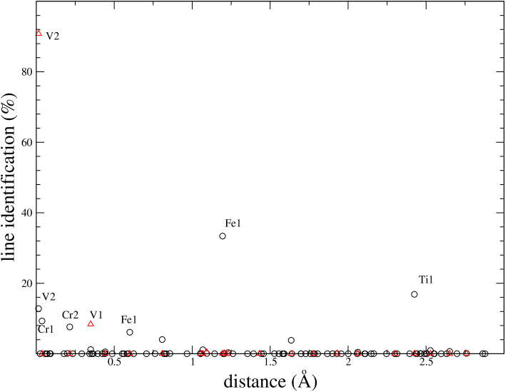
Figure 14: Results of applying our line identification procedure to the deviating point at $2672.018$ Å. The black points assume our best estimate of the abundances of the WASP-12 stellar photosphere, while the red triangles instead apply the analysis with an arbitrary increase in the abundance of vanadium so that it has the same abundance as iron (by number). This makes it clear that the results of our line identification are strongly dependent on the assumptions we make.

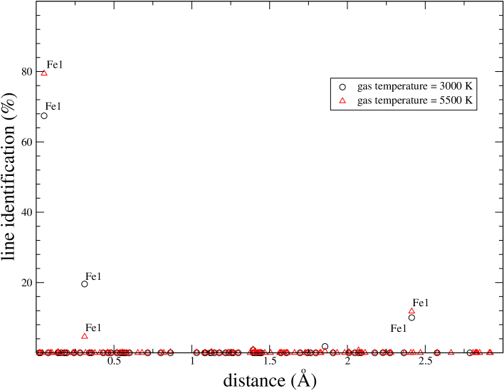
Figure 15: Results of applying our line identification procedure to the deviating point at $2806.933-T5500$ Å. The two sets of points correspond to 3000 K and 5500 K. This makes it clear that the results of our line identifications depend on the temperature as well as the abundance pattern assumed for the absorbing gas.

Fig. 15 shows an example of how the imputed line differs for values of 3000 K and 5500 K in $P_{\chi}$, both plausible values for the exosphere of WASP-12. None of our clear identifications changed between these two temperatures, but we note we have not included the temperature dependence of the ionisation balance in our assessments.

Figs. 14 and 15 show that our line identifications depend on the assumptions we make. This is generally true in astrophysics, but in more mature fields, we have a sound basis for confidently adopting likely assumptions. For example we have a very good understanding of the physical conditions prevailing in stellar atmospheres, and much high SNR ratio data has been used to hone models such as the one we plotted in Figs. 1 and 11. The study of hot Jupiter exospheres is not so well-developed.

To be sure of all line identifications in WASP-12 b and other hot Jupiters, we need sound assumptions for the likely abundances in the absorbing material, and measurements of its physical properties. Hot Jupiter atmospheres probably have prodigious winds and disequilibrium chemistry which will affect the abundances of the exospheric material (e.g. Moses et al 2011). The models have many degrees of freedom, and for WASP-12 b constraining them will be challenging, as the system is relatively distant (380$\pm$85 pc Fossati et al. 2010b) and hence at the limit of what we can do with HST/COS. WASP-12 b is roughly the most distant exoplanetary system for which NUV transit observations can realistically be obtained with technology available in the forseeable future. The best chance to put our understanding of hot Jupiter exospheres on a firm foundation would be to observe the two brightest hot Jupiters, HD 209458 b and HD 189733 b in the NUV. In some cases, however, we already have robust identifications of spectral lines exhibiting enhanced transit depths in WASP-12 b, for example for the Mg II resonance lines.

3.5 Chromospheric Activity in WASP-12 and Tenuous Gas Surrounding the System

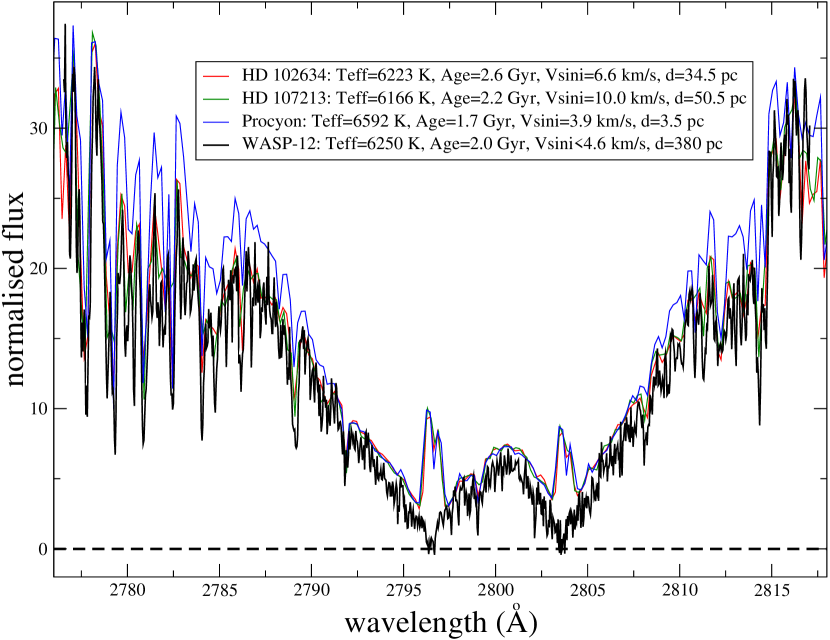
Figure 16: Our Visit 1 NUVC coverage of the cores of the Mg II resonance lines compared with those of three other stars (see text). The cores of the WASP-12 lines show no emission whatsoever, and are suggestive of narrow absorption components which reduce the flux in the cores of these lines to zero. WASP-12 is remarkable in the appearance of its Mg II resonance line cores.

Our HST/COS data raise questions concerning stellar activity in WASP-12. Can we attribute the high point at phase $\phi=0.95$ in the Visit 2 light curves to stellar activity as we speculated in §3.3? Fossati et al. (2010b) found an age of 1.0-2.65 Gyr for WASP-12, and an effective temperature of $T_{\rm eff}=6250\pm 100\,{\rm K}$, in agreement with Hebb et al. (2009) but with tighter uncertainties. Generally, stars of this $T_{\mathrm{eff}}$ and age are expected to exhibit activity, and emission cores in the MgII resonance lines are one clear observable consequence of this. As Figure 16 demonstrates, however, MgII emission cores are conspicuously absent in WASP-12.

To produce Figure 16 we normalised the spectra of WASP-12 and two stars of the same age and $T_{\mathrm{eff}}$ to match the flux in the far wings of the Mg II lines (the regions used in the normalisation are further from the line cores than the edges of Fig. 16). These two stars, HD 102634 and HD 107213, are plotted in red and green in Fig. 16. As expected for such similar stars, the line profiles of WASP-12, HD 102634 and HD 107213 match well throughout the profile of the Mg II lines, except within about $10\,\AA$ of either of the line cores, where WASP-12’s spectrum lies below the others. Fig. 16 also shows Procyon, which is a commonly used reference star, slightly hotter, slightly younger and more slowly rotating ($v\sin i=3.9\,{\rm km\,s}^{-1}$, Schroder, Reiners & Schmitt 2009) than the other three objects. Procyon is noted for its low stellar activity. Procyon, HD 102634 and HD 107213 all have very similar line profiles between $2792\,\AA$ and $2807\,\AA$, with similar emission cores in all three cases surrounded by fairly steep declines in flux towards the line cores, with very similar gradients in all three examples. WASP-12 has anomalously low fluxes within about $10\,\AA$ of the Mg II line cores, with steeper gradients towards the line cores and absolutely no sign of emission in the line cores.

Figure 16 shows that WASP-12, HD 102634 and HD 107312, which have similar ages and temperatures, match extremely well, except for in the line cores. Indeed, the WASP-12 line cores show no sign of the anticipated emission reversals, and appear essentially as saturated absorption profiles: the line cores have zero flux. As the point-to-point deviations in the WASP-12 spectrum make clear, we would definitely have detected emission cores in WASP-12 if even if they were present at a strength significantly less than that in the three comparison stars. Even if WASP-12 were a slowly-rotating sub-giant, Mg II emission cores would be expected (Ayres 2010). Even very inactive Sun-like stars have significant chromospheric spectra with prominent Mg II emission powered by acoustic shock heating and local dynamo action which converts hydrodynamic turbulence into magnetic flux.

Our interpretation of Fig. 16 is that the inner parts of WASP-12’s Mg II lines are absorbed by gas beyond the stellar chromosphere, with sufficient column density to completely obliterate the expected emission reversals, and to perhaps also depress the line wings just outside the cores. Because the star is distant, one possibility is interstellar absorption. As we demonstrate below, however, the necessary Mg⁺ column density is quite substantial, and is implausible unless the ISM in that direction is unusual. Another possibility, which we favor, is that the absorption is local to the WASP-12 system.

Gas immediately surrounding WASP-12 b cannot account for the absorption we have just described. The planet itself covers only a small fraction of the stellar disc: to completely remove the predicted Mg II chromospheric emission would require a much more spatially extended distribution of absorbing material, blanketing the entire stellar disc. We propose, in fact, that the entire system is shrouded in diffuse gas, very likely stripped from WASP-12 b itself under the harsh radiation and stellar wind conditions so close to the parent star. Knutson, Howard & Isaacson (2010) measured the Ca II H & K emission lines of 50 transiting planet host stars including WASP-12. WASP-12’s Ca II H & K lines are completely devoid of detected emission cores, as are the majority of Knutson, Howard & Isaacson (2010)’s sample. Knutson, Howard & Isaacson (2010) interpreted their results in terms of a correlation between stellar activity and hot Jupiter atmosphere type, but our hypothesis suggests an alternative/additional explanation. Many of these systems could be shrouded in diffuse gas which absorbs any emission cores produced by stellar activity.

Chromospheric activity is strongly correlated with stellar age and rotational velocity. WASP-12’s rotational velocity is unknown, but the transit of WASP-12 b is accompanied by an undetected Rossiter-McLaughlin (RM) effect (Husnoo et al. 2011), so either the rotational velocity is low or the orbital angular momentum of WASP-12 b is misaligned with the stellar rotation axis (see e.g. Haswell 2010, for explanation). If the chromospheric activity is low, as expected for a middle-aged slowly rotating dwarf, a stellar flare is a very unlikely explanation for the high flux in orbit 3 of our Visit 2 light curves. We must then conclude either our data are intrinsically noisy beyond the assigned photometric error, or that we are viewing WASP-12 through diffuse gas at all observed orbital phases, and there happened to be a relatively clear view to the stellar surface during orbit 3 of Visit 2. This latter possibility might be produced by a bow shock in a very extended planetary magnetosphere (Vidotto, Jardine & Helling 2011).

3.6 Resonance Line Absorption in WASP-12 and the ISM

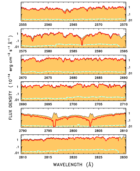
Figure 17: Our WASP-12 NUV spectrum (red) in comparison to that of $\alpha$ Cen (black line, filled beneath). A logarithmic flux scale has been adopted to emphasize the deepest absorption. The green dotted line indicates the errors on the WASP-12 spectrum: data are truncated at levels consistent with zero flux.

Figure 17 shows our Visit 2 WASP-12 spectrum compared to HST/STIS data on $\alpha$ Cen from the archive. The STIS data have been convolved with the COS NUV LSF and scaled by the multiplicative factor $4\times 10^{-5}$. Both spectra have been smoothed for display purposes. The flux axis is logarithmic to emphasize the deep absorption in the cores of strong lines. The photometric error is per resolution element, and the flux densities have been truncated at the $1\,\sigma$ error level. As in Fig. 16, the spectra have been normalised to agree in the far wings of the Mg II absorption. Generally stellar Mg II line profiles scale so that normalising in the far wings produces good agreement in the inner wings for stars of the same luminosity class (Ayres 2010), but as we saw in Fig. 16, WASP-12’s inner wings are depressed relative to other main sequence stars. The Mg II resonance line cores in WASP-12 have total absorption, which is perhaps blue-shifted by $\sim$ 20 $\mathrm{km\,s}^{-1}$.

In the NUVA region of Fig. 17, WASP-12 exhibits similar total absorption in the core of the Fe II resonance line at $\lambda$2586 Å  where $\alpha$ Cen’s absorption is shallower by over a factor of 10. Appearing slightly less strong is WASP-12’s Mn II resonance line at $\lambda$2577 Å.

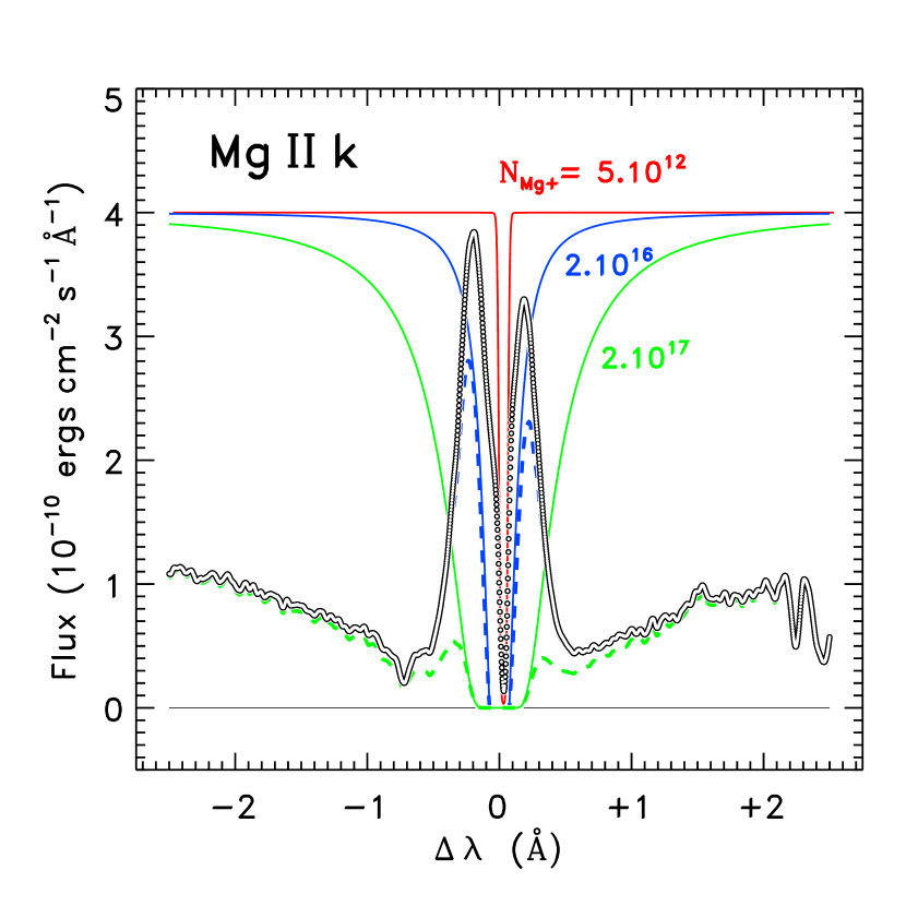
Figure 18: Calculations of interstellar absorption applied to the center of the Mg II line profile of $\alpha$ Cen. The observed line profile is plotted as open circles which overlap to form a double line; the solid lines show the predicted absorption for column densities of N$(Mg^{+})$ of $5\times 10^{12}\,{\rm cm^{-2}}$ (red), $2\times 10^{16}\,{\rm cm^{-2}}$ (blue) and $2\times 10^{17}\,{\rm cm^{-2}}$ (green). The modified line profiles produced by applying the two higher column densities are indicated in dashed lines of corresponding colour.

These absorption features in the WASP-12 stellar spectrum are too deep to have their origin in the photosphere itself. Our favoured interpretation is that the absorption arises in gas within the WASP-12 system, but we now examine the plausibility of the alternative explanation that the absorption might arise in the ISM. Figure 18 shows the central part of the observed $\alpha$ Cen A Mg II k-line profile. The solid red line shows the absorption we expect from the ISM along the very short pathlength (1.3 pc) to the star, using the Mg II column density of $5\times 10^{12}$ cm^-2 reported by Linsky & Wood (1996). The absorption profile was calculated using a temperature of 7000 K and a turbulent velocity of 1.5 km/s, typical values for the local warm cloud in which $\alpha$ Cen A and the Sun are embedded. The calculated absorption fits the narrow slightly redshifted absorption dip in the extreme core of the line, noting that the broader “absorption” between the twin peaks of the profile is a central reversal of chromospheric origin (see Linsky & Wood 1996). The blue curve indicates the attenuation predicted for a plausible N(Mg⁺) in the line of sight to WASP-12: $2\times 10^{16}$ cm^-2. We arrived at this estimate assuming $E(B-V)\sim 0.2$ magnitudes for WASP-12 (based on a nominal 0.6 magnitudes kpc^-1 of reddening for an average Galactic sightline and the $\sim 350$ pc estimated distance of WASP-12), which yields a hydrogen column density of $\sim 1.2\times 10^{21}$ from the standard Milky Way reddening law (e.g., Savage & Mathis 1979). If we then assume that roughly half the magnesium is in the form of Mg⁺ — about what is deduced from the $\alpha$ Cen A sightline, albeit perhaps not typical — then we obtain: $N(Mg^{+})\sim 2\times 10^{16}$ cm^-2. Applying the corresponding absorption profile to the $\alpha$ Cen A Mg II k line results in the dashed blue curve, which still preserves substantial core emission.

The green line in Fig. 16 depicts the absorption profile for a Mg II column density a factor of 10 greater than the interstellar estimate above, i.e. $N(Mg^{+})=2\times 10^{17}$ cm^-2. Here broad damping wings have developed, strongly suppressing the emission core, and even affecting the inner wings of the k line. While the predicted profile is not an exact match to that of WASP-12 (cf., Fig. 14), it does demonstrate the plausibility of the absorption mechanism, albeit requiring a very substantial column of Mg⁺. The required column is excessive enough, in fact, to make an interstellar origin seem much less plausible than a more local source, especially given the existence of the hot Jupiter and the possibility of strong atmospheric stripping. We examine this possibility in more detail later (§4.2, below).

4 Discussion and Conclusions

The conclusions we reached in Paper 1 more or less stand in the light of our Visit 2 data and our interpretation of the entire COS/NUV dataset. As §3 shows, the Visit 2 data did not neatly fill in the phase-folded NUV light curves we produced from Visit 1. Instead, a rather more complex reinterpretation was required. Our principle conclusions in Paper 1 (from Visit 1 data alone) were that the NUV transit depth is deeper than the optical, that this is due to absorption in metal atoms/ions within WASP-12 b’s exosphere, and that this exospheric gas was spatially distributed such that an early ingress occurs. To make sense of our combined NUV light curves, we needed to adopt two further hypotheses: (i) the absorbing gas is (at least sometimes) even more spatially extended than we inferred from Visit 1; (ii) a short-lived stellar flare occurred during Visit 2 orbit 3 or Visit 2 orbit 3 had a line of sight through a relatively low density window in the absorbing gas.

In Section 3 we presented several lines of indirect evidence in favour of the hypothesis that WASP-12 has some chromospheric activity, despite the resounding lack of observed emission cores in the Mg II and Ca II lines. We now examine our data to see if it contains direct evidence in favor of this hypothesis over the alternative low density window hypothesis.

4.1 A stellar flare during Visit 2 orbit 3?

We have attributed the high NUV fluxes during Visit 2 orbit 3 to a stellar flare. To check this interpretation, Fig. 19 shows a direct comparison of the NUV spectra from orbit 3 of Visit 2 with orbit 3 of Visit 1. The two spectra are plotted with the pipeline calibration, no normalisation was applied to account for the declining throughput. These spectra are clearly noisier that those shown in earlier figures as they comprise only about a fifth of the exposure time on each visit. The two spectra broadly agree, but there is a hint in the Visit 2 spectrum of a small emission component redwards of the center of each of the Mg II line cores. This is not an unassailable detection. The appearance of these two small bumps is very similar to the remnant line core emission on the red side of the line profile in Figure 18 after application of absorption by a column of N${\rm(Mg^{+})}=2\times 10^{17}\,{\rm cm^{-2}}$. The remnant emission on the blue side of the line core is absent in Fig. 19, but as we noted in our description of Fig. 17, the absorption in WASP-12’s line cores appears slightly blue-shifted (by about $0.25\AA$) relative to the photospheric spectral lines. The damping wings of a blue-shifted absorption profile (see Figure 18) would extinguish the blue side of the emission core before the red side.

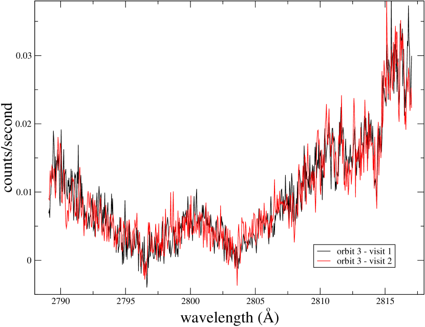
Figure 19: A direct comparison of the NUVC overlapping spectral region in orbit 3 of each the two visits.

Thus Fig. 19 provides us with (noisy) direct evidence for chromospheric emission in the Mg II line cores. Further it shows an increase in this emission or a decrease in the absorption between the stellar chromosphere and the telescope during Visit 2 orbit 3.

The dramatic movement of the Visit 2 orbit 3 NUVA data point when Figs. 5 and 9 (or Figs.  7 and  8) are compared suggests we are seeing a veiled stellar flare rather than a low density window. In Figs. 5 and  8 the Fe II resonance line at $\lambda$2586 Å is included, and the flux is high. In Figs. 7 and  9, this line is excluded and the flux is much lower. A flare would increase the chromospheric emission in the Mg II and Fe II resonance lines. When the NUVA data excludes the Fe II line (Fig. 9) there is no sign of a high point in the photometry. It is only where chromospheric activity indicators are included within the passband, i.e. always in NUVC (Figs. 5,  7,  8 and  9) and in NUVA in Figs. 5 and 8 but not Figs. 7 and 9, that the light curve has a high point. We infer that the enhanced chromospheric emission in Fe II is absorbed by the obscuring gas, and re-emitted isotropically and across the line profile. Thus the line core emission is distributed across the line profile and rendered undetectable at any individual pixel in the spectrum. When we sum over wavelength to produce light curves, however, the signal becomes apparent above the noise.

Since the flux from the stellar photosphere in the Fe II $\lambda$2586 Å  line is low (Fig. 17), whether or not this line is included within the wavelength coverage should make little difference to the light curve in the low density window hypothesis. We therefore interpret the 4$\sigma$ movement of Visit 2 orbit 3 NUVA point between Fig. 7 and Fig. 8, i.e. between data including and excluding this line as evidence in favour of the stellar flare hypothesis over the low density window hypothesis. Only when we include features which we expect to show a significant flux increase during a stellar flare do we see the NUV flux in Visit 2 orbit 3 lying significantly above the other data. Several aspects of our data thus suggest we caught a stellar flare which occurred during the ingress of the optical transit in Visit 2.

4.2 The column density of Mg II

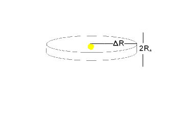
Figure 20: Geometry assumed in our estimate of plausible limits to the column density due to mass loss from WASP-12 b. Material is assumed to be spread within a squat cylinder of radius $\Delta R$ and height $2R_{*}$ centered on the star.

In Section 3.6 we showed that a high column density of Mg II between us and the stellar chromosphere can absorb WASP-12’s Mg II emission cores, assuming the intrinsic emission is similar to that of $\alpha$ Cen. Here we consider whether the value we deduced, N${\rm(Mg^{+})}\sim 2\times 10^{17}\,{\rm cm^{-2}}$, can be plausibly attributed to mass loss from the planet WASP-12 b. Since this extremely close-in planet is the most obviously unusual characteristic of the star, it seems likely that the anomalous Mg II line profiles are ultimately caused by the planet.

Various mechanisms have been proposed for mass loss from WASP-12 b and similar planets. There are several variants of the ‘blow-off’ hypothesis, which assumes hydrodynamic outflow driven by energy input from irradiation by the host star. Tidal heating can drive planetary envelope expansion and consequent Roche lobe overflow (Li et al 2010). For the early eccentricity estimates of WASP-12 b, for example, this mechanism was predicted to cause a mass loss rate of $10^{-7}\,{\rm M_{J}\,yr^{-1}}$ (ibid).

Mass lost from the planet will carry specific angular momentum from the planet’s orbit, and will thus tend to be confined to the orbital plane. To absorb chromospheric emission from the entire visible disc of the star, the material must extend about one stellar radius above and below the orbital plane. To derive an upper limit on the absorbing column density due to mass lost from the planet, therefore, we begin with the geometry shown in Fig. 20. Gas is present within a squat cylinder of radius $\Delta R$ and height $2R_{*}$, centered on the star and aligned with the orbital plane.

The mean density, $\bar{\rho}$ within the cylinder is

$$\bar{\rho}\leq\frac{\dot{m}\Delta t}{2\pi\Delta R^{2}R_{*}}$$ (5)

where $\dot{m}$ is the mass loss rate and $\Delta t$ is the time over which mass has been lost. The equality arises when all mass lost from the planet is confined to the cylinder we require to be populated. This is obviously an upper limit as some mass will accrete on to the star or diffuse in the vertical direction out of our line of sight to the star.

The column density of particles is

$$N_{tot}\leq\int_{{\rm LOS}}\frac{\rho}{\mu}\,{\rm d}l\approx\frac{\dot{m}\Delta t}{2\pi\Delta RR_{*}\mu}\approx\frac{\dot{m}}{2\pi vR_{*}\mu}$$ (6)

where the integral is carried out along our line of sight (LOS), $\mu$ is the mean molecular weight of the gas and $v=\Delta R/\Delta t$ is the velocity with which the gas moves outwards from the orbit of the planet. We have used the mean density and implicitly assumed that the velocity is approximately constant for outflow over the distance $\Delta R$. The integral is effectively performed over the distance $\Delta R$ which contributes appreciably to the column density. This avoids addressing our ignorance of the functions $\rho(l)$ and $v(l)$. The approximations are sufficient for an order of magnitude estimate, particularly since our empirical estimate of $v$ will ensure our approximation is weighted to the appropriate part of the velocity field. If the fraction of the total number density in the form of Mg II is $f$, then

$$N({\rm Mg^{+}})\leq\frac{\dot{m}f}{2\pi vR_{*}\mu}$$ (7)

To obtain $N({\rm Mg^{+}})$, we adopt the mass loss rate predicted by evaporation processes, for example Ehrenreich and Desert (2011) give $\dot{m}\sim 3\times 10^{7}{\rm kg\,s^{-1}}$ for WASP-12 b. We take $f\approx 10^{-5}$, which is based on a number fraction of $10^{-4}$ for Mg in the solar elemental abundance mix, and a (conservative) assumption that one in 10 magnesium nuclei is in the Mg II ionic state; $R_{*}=1.1\times 10^{9}\,{\rm m}$ (Chan et al 2011); we assume a mean molecular weight of $\mu={\rm m_{\rm p}=1.7\times 10^{-27}\,{\rm kg}}$ which will be correct to within a factor of a few for material predominately composed of hydrogen. We can estimate $v$ from our data: the absorption appears to be blue-shifted by roughly $0.25\AA$ (Fig. 17, 5th panel from the top), implying $v\sim 2.5\times 10^{4}{\rm m\,s^{-1}}$ Using these values in Eqn. 7 we obtain $N({\rm Mg^{+}})\leq 4\times 10^{21}\,{\rm cm^{-2}}$. The required column density is below this crude upper limit by a factor of $\sim 2\times 10^{4}$. Obviously, some material will move inwards and be captured by the star, and some will spread in the vertical direction beyond the cylinder we require to be filled with gas, but we have a comfortable factor to allow for this and other losses of Mg II.

4.3 Exospheric Gas or Coronal Gas?

WASP-12 b is only about one stellar diameter from the stellar surface, so this planet is orbiting within the star’s corona. This raises the possibility that absorption we observed around WASP-12b may be attributable to entrained or bow-shocked coronal gas, rather than from mass lost from the planet (e.g. Vidotto, Jardine & Helling 2010, 2011). Indeed Vidotto, Jardine & Helling (2011) show how a ‘double’ transit can arise if a transiting planet is preceded by a bow shock in a very extended planetary magnetosphere. This does not completely explain our Visit 2 light curves as the observed absorption begins very early and the curves which do not contain activity-indicating lines differ in shape from those which do (see § 4.1). The typical coronal temperatures at the distance of the planet are, however, probably inconsistent with the absorption we detect. Fig. 11 gives us very strong indications that the absorption causing our NUV transit is from gas at a similar temperature to the stellar photosphere. The densities in the gas causing the NUV transit exceed those of a typical stellar corona (otherwise the NUV transit would be indistinguishable from the optical transit), so naturally, by energy arguments, the temperature of this gas is lower. This argument does not, however, rule out entrainment of coronal gas by the planet. § 4.2 strongly suggests, however, that most of the gas around WASP-12 is due to mass loss from the planet: stars without extreme planets like WASP-12 b offer us clear sight of their Mg II chromospheric emission cores. Our observations show the emission cores are completely absorbed throughout our temporal coverage. This requires gas at considerable distances from the planet itself.

4.4 The Roche lobe of WASP-12 b

Fig. 21 shows the Roche lobe of WASP-12 b. The y-z cross-section is approximately that presented to us during transit; $i=86^{\circ}\pm 3^{\circ}$ (Chan et al 2011), so the y-z plane is inclined to the plane of the sky by $4^{\circ}\pm 3^{\circ}$. The lowest panel of Fig. 21 shows the cross-section of the critical equipotential surface is not much larger than that of the planet itself. We have detected transit depths in the NUVA and NUVC spectra regions which are up to a factor of 3 deeper than the optical transit (see Figs. 5 and 9). As the optical depth of the absorbing gas will vary with both wavelength and position, it is clear that we require the projection of the spatial distribution of the absorbing gas on the plane of the sky to exceed that of the Roche lobe by a factor of more than a few. Our observations thus show that the absorbing gas far overfills the planet’s Roche lobe. This is consistent with our Visit 2 data, which suggest absorption is occurring at phase 0.83 (see Fig. 8), i.e. the absorbing gas extends $\sim 20\%$ of the way around the orbit.

Figure 21: The Roche lobe of WASP-12. The y-z cross-section (lowest panel) is presented to us during transit. The solid black lines indicate the equipotential surface defined by the area determined by the optical transit. A fluid planet will fill this surface. The dotted circles have area equal to the y-z cross-section of the planet. The dashed lines show the critical equipotential surface which delimits the planet’s Roche lobe.

Fig. 21 also shows the deviation from spherical of WASP-12 b. The fluid planet will fill the equipotential surface corresponding to the area occulted in the optical transit. The y-z cross-section of this equipotential surface deviates slightly from circular as a result of the centripetal force, with the x-y and x-z cross-sections each being noticeably distorted by the combination of the tidal distortion due to the stellar gravity and the centripetal force. The volume of the planet is consequently $\sim 20\%$ greater than that of a sphere producing the same optical transit depth.

4.5 NUV versus FUV

As we discussed in the introduction, most of the observations of diffuse gas around hot Jupiter exoplanets have been carried out in the FUV, with our WASP-12 program being the single published exception. Our observations are clearly limited by the SNR of the data, but it must be remembered that WASP-12 is 4 magnitudes fainter than either HD 209458 b or HD 189733 b, the two objects where FUV transit observations exist. Even with the 4 magnitudes advantage, conclusions from the FUV transit data can be compromised by the fact that the FUV stellar emission is patchy and variable in time and/or severely limited by poor SNR. To demonstrate how FUV observations can be irrevocably compromised by these issues, we present a brief case study using FUV COS data. The target, HD 189733 b, is a hot Jupiter transiting a bright nearby early K-star, and has been widely and informatively studied.

The observations were obtained on 16 September 2009 as part of HST program 11673. The data were acquired with the FUV G130M mode (Osterman et al. 2011), spanning 1134 $\leq$ $\lambda$ $\leq$ 1429 Å at a velocity resolution of $\approx$ 17 km s ^-1. A total of 9.9 ksec of exposure time was obtained over five spacecraft orbits, allowing time for instrumental settling and stabilization (see Vidal-Madjar et al. 2004 and references therein) prior to the transit observations. Observations covered orbital phases from -0.074 to 0.051 (adopting the orbital parameters of Knutson et al. 2007). The data were obtained from the Multi-Mission Archive at STScI (MAST) and calibrated one-dimensional spectra were coadded with the custom IDL procedures described by Danforth et al. (2010). The coadded spectrum is displayed in Fig. 22. The SNR per resolution element is $>50$ in the chromospheric CII 1334, 1335 A lines.

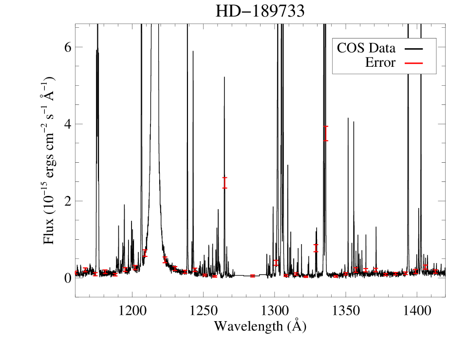
Figure 22: Coadded far-UV observations of the well-studied exoplanet host HD 189733, obtained with the $HST$-Cosmic Origins Spectrograph. Despite the relatively low flux levels, COS can produce high SNR emission line spectra of planet host stars.

As COS is a slitless spectrograph, geocoronal emission complicates observations at discrete wavelengths (most notably H I Ly$\alpha$, 1216 Å, and the O I multiplet at 1304 Å). However, the high sensitivity and low instrumental background allow high-SNR observations in emission lines of several other chromospheric and transition region ions, including C III $\lambda$1175, Si III $\lambda$1206, N V $\lambda$1240, C II $\lambda$1335, and Si IV $\lambda$1400. Unfortunately the very processes powering these emission lines (e.g., Ayres & France 2010) also limit the capability of far-UV transit studies.

Light curves of the bright chromospheric emission lines from the spectrum in Fig. 22 were created from the calibrated two-dimensional data by exploiting the TIME-TAG capability (France et al. 2010). These are shown in Fig. 23. We extracted an [$x_{i}$,$y_{i}$,$t_{i}$] photon list from each exposure $i$ and coadded these to create a master [$x$,$y$,$t$] photon list. The total number of counts in a [$\Delta$$x$,$\Delta$$y$] box was integrated over a timestep of 120s. The instrument background level is computed in a similar manner, with the background integrated over the same wavelength interval as the emission lines, but offset below the active science region. The instrumental background is $<$ 6% of the total line flux for all species presented in Fig. 23. Following the extraction of the light curves in photons s^-1, the data are normalized for a relative comparison of the line flux as a function of time. For each species, we created a linear fit to the out-of-transit light curves (orbital phase $<$ -0.015 and $>$ 0.030), excluding time bins at the beginning or end of an orbit. This is similar to the normalisation procedure adopted in Paper 1 and in Fig 2. These normalized light curves are plotted in Fig. 23. The variation on timescales of minutes to hours is significantly larger than the statistical error in an individual bin.

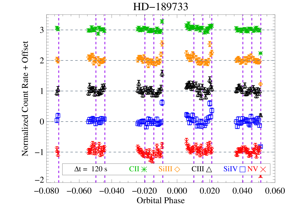
Figure 23: Count rates of the brightest far-UV emission lines not contaminated by geocoronal airglow (e.g, H I Ly$\alpha$ and O I $\lambda$1304). The light curves were created from the two-dimensional COS data files, with the total number of counts in given line (defined by an [$x$,$y$] location on the COS detector) integrated in 120s intervals. Error bars are taken to be the square-root of the number of counts in a given time bin. We note that the variability on minute to hour timescales exceeds the photon noise and can be the limiting factor for transit studies of chromospherically active, low-mass stars. The dashed lines denote the end of an individual COS exposure.

If we assume that exposures taken on the fourth spacecraft orbit represent the in-transit spectrum, we can compare the coadded, one-dimensional in-transit and out-of-transit spectra. Integrating the total flux over airglow-free wavelength intervals, $\Delta\lambda$ = [1150 – 1210 Å, 1220 – 1270 Å, 1308 – 1425 Å], we find a in-transit/out-of-transit flux ratio of 1.000 $\pm$ 0.017. These FUV observations therefore give no detection of the transit. Other FUV transit observations have given more reliable information, partly because HD 209458 is an older, solar-type star with less activity than HD 189733, but any FUV light curve results from the unknown and un-reproducible locus of the transit light curve across the patchy and changing stellar chromospheric emission distribution (Haswell, 2010). Lecavelier Des Etangs et al (2012) report STIS FUV observations of two transits of HD 189733 b. They too fail to detect the transit in observations made in 2010 April. In 2011 September the STIS observations were accompanied by contemporaneous X-ray observations in which stellar flaring activity was detected. This time the Lyman $\alpha$ profile showed variations attributed to exospheric absorption, but no signal was detected in Si III, O V or N V. Lecavelier Des Etangs et al (2012), perhaps because of the brevity required for a Letter, give no assessment of the variability inherent in the observed stellar Lyman $\alpha$ emission. Intriguingly, the X-ray lightcurve of Lecavelier Des Etangs et al (2012) shows a high point during optical ingress which is reminiscent of our Visit 2 NUVA and NUVC orbit 3 anomaly.

Like the FUV observations of HD 189733, our Visit 2 NUV light curve of WASP-12 was also complicated by stellar activity, but we were able to isolate and ameliorate its effect (c.f. the NUVA lightcurve in Fig. 9). The NUV can provide more robust information on absorption by diffuse gas than the FUV. The COS/FUV observations of HD 209458 b (Linsky et al. 2010) have exquisitely high SNR; NUV observations of this planet would clearly reveal much information about the composition and velocity structure of its exosphere.

4.6 Summary

1. We observed WASP-12 in the NUV, a spectral region which proves to be an extremely sensitive probe for the presence of absorbing gas.

2. We have detected asymmetric absorbing material in the WASP-12 system which is more extensive than the Roche lobe of WASP-12 b.

3. The stellar photospheric absorption appears to be a fairly good predictor of the wavelength-dependence of the excess absorption, indicating the extended gas may be similar in composition and ionisation state to the WASP-12 photosphere. The NUVB spectral region, which has the least photospheric absorption and is devoid of strong resonance lines yields the most straight-forward light curve. This gives us confidence in our interpretation.

4. In HST Visit 1 we detected enhanced absorption during and before the optical transit.

5. In HST Visit 2 our NUV light curve appeared to be below the out-of-transit flux level for all the pre-ingress coverage, despite this extending to earlier phases than that of Visit 1. Thus the spatial distribution of the absorbing gas appears to vary.

6. The cores of the Mg II and Fe II resonance lines are very dark throughout our coverage. WASP-12 would be completely unique amongst all stars of similar age and spectral type if this lack of observed Mg II chromospheric emission reversals was intrinsic to the star. We attribute it instead to absorption occurring in gas between us and WASP-12. The required column density is at least $\sim 2\times 10^{17}$ cm^-2. This value is about a factor of 10 greater than a plausible estimate of the interstellar column density, but is consistent with gas loss from WASP-12 b via photo-evaporation. Nevertheless, the ISM explanation cannot be dismissed completely, since there is substantial “cosmic variance” in ISM properties, and the WASP-12 sightline might just be unusually opaque in Mg II.

7. The lack of Mg II chromospheric emission cores from the star could be explained by absorbing gas not confined to the region immediately surrounding the planet. Absorbing gas would need to occupy the lines-of-sight to at least the mid-latitude regions of the stellar disc at all orbital phases. We show that an outflow of some fraction of the mass loss expected from WASP-12 b can plausibly provide this obscuration, though we have not proved the gas will necessarily fulfill the geometric requirements.

8. In HST Visit 2 the NUV flux was near its maximum value at optical ingress. Such a fast change in flux is a signature of a stellar flare, although such an event would be very rare on a low-activity star like WASP-12. Nevertheless, there are (albeit very noisy) hints in the Mg II line profile of some chromospheric emission at this time.

9. FUV transit observations can be far more affected by stellar activity than our NUV observations were. In the NUV we have the opportunity to isolate the effects of activity by excluding spectral lines which are strongly affected.

10. We obtained new optical photometry and combined this with archive optical photometry to derive an improved linear ephemeris

    $$T_{\rm mid}({\rm HJD})=2454852.7739^{+0.00014}_{-0.00014}+N\times 1.09142206^{+0.00000033}_{-0.00000031}$$ (8)

4.7 Concluding remarks

Given its spectral type and probable age, we have suggested that WASP-12 should have a normal level of chromospheric activity, despite the lack of observed emission cores in the Mg II resonance lines. This hypothesis in principle could be tested by obtaining far-UV (FUV) spectra, which should show the normal complement of chromospheric (e.g., O I 1305 Å triplet; C II 1335 Å multiplet) and higher-temperature features (e.g., C IV 1550 Å doublet). However, the great distance of WASP-12 (at least 300 pc, Fossati et al. 2010b) would imply line peak flux densities below $10^{-16}$ erg cm^-2 s${}^{-1}\AA^{-1}$ (scaling from the FUV spectrum of $\alpha$ Cen A), which even with the high sensitivity G140L grating of COS would require an exposure of $\sim 25$ ks to reach a secure S/N$\sim 10$, or nearly 10 HST orbits. Even worse, the estimated interstellar reddening of $E(B-V)\sim 0.2$ magnitudes would imply an additional factor of $\sim 5$ attenuation of the FUV lines, further lengthening the necessary COS or STIS exposures to beyond the realm of practicality. Furthermore, this does not even account for the additional absorption deduced from the WASP-12 Mg II lines, which — if truly interstellar and accompanied by the normal dust-to-gas ratio — would completely extinguish the FUV radiation. Similarly, and again scaling from $\alpha$ Cen A, WASP-12 would be predicted to be a 0.02 counts ks^-1 coronal X-ray source in the Chandra imagers, which is about a factor of two below the average cosmic background rate. In that background-limited regime, it would require at least 1 Ms of exposure to achieve a minimal 3$\,\sigma$ detection, again completely impractical.

We need to look at more close-in exoplanets using this highly informative NUV wavelength region. Most known hot Jupiters are less distant than WASP-12, and consequently will offer higher NUV fluxes and thus better signal to noise. Our conclusions throughout this paper are limited by the noise level in our data.

Many related studies have been performed in the FUV. The FUV does provide access to higher ionization state lines that can be good proxies for activity and suffer less confusion with the lower-ionization ISM (CIII, NV, SiIV). Additionally, the CIII FUV multiplet is not a resonant transition, its lower level lies about 6.5 eV above the ground state, therefore this line is effectively never seen in the diffuse ISM. Despite this, as Fig. 5.10 of Haswell (2010) makes clear, the NUV has some clear advantages over the FUV for studies of exospheric absorbing gas. NUV transits are measured against the relatively uniform and well-understood stellar photospheric light, whereas the FUV emission from the stellar disc is patchy, time-variable, and limited to the wavelengths of strong chromospheric emission lines. In addition to the consequent improvement in robustness of the inferences drawn about the absorbing gas, the NUV also has a huge advantage in stellar flux and thus SNR. There are many open questions and much theoretical and modeling activity connected with the handful of extant UV observations of transiting hot Jupiters. It is vital that more UV transit observations are made while HST remains available.

References

- Adams (2011) Adams, F.C. 2011 ApJ730, 27
- Ayres (2010) Ayres, T. 2010, Mem. Soc. Astron. Italiana, 81, 553
- Ben-Jaffel (2007) Ben-Jaffel, L. 2007, ApJ, 671, L61
- Carter & Winn (2009) Carter, J. A. & Winn, J. N. 2009, ApJ704, 51
- Chan et al (2011) Chan,T., Ingemyr, M., Winn, J.N., Holman, M.J., Sanchis-Ojeda, R., Esquerdo, G., Everett, M. 2011, AJ, 141, 179
- Collier Cameron et al. (2007) Collier Cameron, A. et al. 2007, MNRAS, 380, 1230
- Desert et al. (2008) Desert, J.-M., Vidal-Madjar, A., Lecavalier des Etangs, A., Sing, D., Ehrenreich, D., Ferlet, R. 2008, A&A, 492, 585.
- Ehrenreich and Desert (2011) Ehrenreich, D. Desert, J.-M. 2011, A&A, 529, A136.
- Ekenbäck et al. (2010) Ekenbäck, A., Holmström, M., Wurz, P., et al. 2010, ApJ, 709, 670
- Enoch et al. (2010) Enoch, B. et al. 2010, A&A, 516, 33
- Erkaev et al. (2007) Erkaev, N. V., Kulikov, Yu. N., Lammer, H., Selsis, F., Langmayr, D., Jaritz, G. F., Biernat, H. K. 2007, A&A, 472, 329
- Fortney et al. (2010) Fortney, J.J., Shabram, M., Showman, A.P., Lian, Y., Freedamn, R.S., Marley, M.S., Lewis, N.K. 2010, ApJ, 709, 149
- Fossati et al. (2010a) Fossati, L., et al. 2010a, ApJ, 714L, 222
- Fossati et al. (2010b) Fossati, L., et al. 2010b, ApJ, 720, 872
- Gazak et al. (2011) Gazak, J. Z. et al. 2011, (arXiv:1102.1036)
- Green et al. (2012) Green, J. C., Froning, C. S., Osterman, S., et al. 2012, ApJ, 744, 60
- Guo (2011) Guo, J.H. 2011, ApJ733, 98
- Haswell, (2010) Haswell, C. 2010, ’Transiting exoplanets’, CUP ISBN 978-0521139380.
- Hebb et al. (2009) Hebb, L., et al. 2009, ApJ, 693, 1920
- Holmes et al. (2011) Holmes, S., et al. 2011, PASP, submitted. See pirate.open.ac.uk/publications
- Holmström et al. (2008) Holmström, M., Ekenbäck, A., Selsis, F., et al. 2008, Nature, 451, 970
- Husnoo et al (2011) Husnoo, N., Pont, F., Hébrard, G., Simpson, E., Mazeh, T., Bouchy, F., Moutou, C., Arnold, L., Boisse, I., Díaz, R.F., Eggenberger, A., Shporer, A. 2011, MNRAS, 413, 2500.
- Irwin & Lewis (2001) Irwin, Lewis
- Knutson, Howard & Isaacson (2010) Knutson, H.A., Howard, A.W., Isaacson, H. 2010, ApJ, 720, 1569
- Kochukhov (2007) Kochukhov, O. 2007, Proc. Int. Conf., Physics of Magnetic Stars, ed. I. I. Romanyuk & D. O. Kudryavtsev, 109
- Kupka et al. (1999) Kupka, F., Piskunov, N., Ryabchikova, T. A., Stempels, H. C., & Weiss, W. W. 1999, A&AS, 138, 119
- Lai et al (2010) Lai, D., Helling, Ch., van den Heuvel, E.P.J. 2010 ApJ, 721, 923
- Llama et al (2011) Llama, J., Wood, K., Jardine, M., Vidotto, A.A., Helling, Ch., Fossati, L., Haswell, C.A. 2001 MNRAS, in prep; arXiv:1106.2935
- Lecavelier Des Etangs et al (2010) Lecavelier Des Etangs, Ehrenreich, D., Vidal-Madjar, A., Ballester, G.E., Desert, J.-M., Ferlet, R., Hebrard, G., Sing, D.K., Tchakoumegni, K.-O., Udry, S. 2010, A&A, 514, 72
- Lecavelier Des Etangs (2007) Lecavelier Des Etangs, A. 2007, A&A, 461, 1185.
- Lecavelier Des Etangs et al (2004) Lecavelier Des Etangs, A., Vidal-Madjar, A., McConnell, J.C., Hebrard, G. 2004, A&A, 418, 1
- Lecavelier Des Etangs et al (2012) Lecavelier Des Etangs, A., Bourrier, V., Wheatley, P.J., Dupuy, H., Ehrenreich, D., Vidal-Madjar, A., Hébrard, G., Ballester, G.E., Désert, J.-M., Ferlet, R., Sing, D.K. 2012, A&A. 543, L4 (arXiv:1206.6274)
- Li et al. (2010) Li, S., Miller, N., Lin, D. N. C. & Fortney, J. J. 2010, Nature, 463, 1054
- Linsky & Wood (1996) Linsky, J. L., & Wood, B. E. 1996, ApJ, 463, 254
- Linsky et al. (2010) Linsky, J.L., Yang, H., France, K., Froning, C.S., Green, J.C., Stocke, J.T., Osterman, S.N. 2010 ApJ717, 1291
- Lopez-Morales et al (2009) Lopez-Morales M., Coughlin J. L., Sing D. K., Burrows A., Apai D., Rogers J. C., Spiegel D. S., Adams E. R., 2010, ApJ, 716, L36
- Maciejewski et al (2011) Maciejewski, G., Errmann, R., Raetz, St., Seeliger, M., Spaleniak, I., & Neuhauser, R. 2011, A&A, 528, A65.
- Miller et al (2012) Miller, B.P., Gallo, E., Wright, J.T., Dupree, A.K. 2012 ApJin press arXiV:1206.0746
- Moses et al (2011) Moses, J.I., Visscher, C., Fortney, J.J., Showman, A.P., Lewis, N.K., Griffith, C.A., Klippenstein, S.J., Shabram, M., Friedson, A.J., Marley, M.S., Freedman, R.S. 2011, ApJin press arXiv:1102.0063.
- Martinez-Arnaiz et al (2010) Martinez-Arnaiz, J., Maldonado, J., Montes, D., Eiroa, C., Montesinos, B. 2010, A&A, 520, A79.
- Osten et al (2011) Osten, R., Massa, D., Bostroem, A., Aloisis, A., Proffitt, C. 2010 Instrument Science Report COS 2011-02. Baltimore: STScI.
- Osten et al (2010) Osten, R., Ghavmian, P., Nemi, S.-M., Massa, D., Penton, S., Aloisi, A., Keyes, C., Osterman, S., Proffitt, C. 2010 Instrument Science Report COS 2010-15 (v1). Baltimore: STScI.
- Osterman et al. (2011) Osterman, S., Green, J., Froning, C. et al. 2011, Ap&SS, 335, 257
- Piskunov et al. (1995) Piskunov, N. E., Kupka, F., Ryabchikova, T. A., Weiss, W. W., & Jeffery, C. S. 1995, A&AS, 112, 525
- Raiput & Safvan (2011) Raiput, J. & Safvan, C.P. 2011, J. Chem. Phys., 134, 201101
- Ryabchikova et al. (1999) Ryabchikova, T. A., Piskunov, N. E., Stempels, H. C., Kupka, F., & Weiss, W. W. 1999, Phis. Scr., T83, 162
- Savage & Mathis (1979) Savage, B. D., & Mathis, J. S. 1979, ARA&A, 17, 73
- Schroder, Reiners & Schmitt (2009) Schroder, C., Reiners, A., Schmitt, J.H.M.M. 2009, A&A, 493, 1099
- Speigel et al. (2010) Spiegel, D.S., Burrows, A., Ibgui, L., Hubeny, I., Milsom, J.A. 2010, ApJ, 709, 149
- Shulyak et al. (2004) Shulyak, D., Tsymbal, V., Ryabchikova, T., Stütz, Ch., & Weiss, W. W. 2004, A&A, 428, 993
- Tremblin & Chiang (2012) Tremblin, P., Chiang, E. 2012 arXiv:1206.5003
- Vidal-Madjar et al. (2003) Vidal-Madjar, A., Lecavelier des Etangs, A., Désert, J.-M., et al. 2003, Nature, 422, 143
- Vidal-Madjar et al. (2004) Vidal-Madjar, A., Désert, J.-M., Lecavelier des Etangs, A., et al. 2004, ApJ, 604L, 69
- Vidal-Madjar et al. (2008) Vidal-Madjar, A., Lecavelier des Etangs, A., Désert, J.-M., et al. 2008, ApJ, 676, L57
- Vidotto, Jardine & Helling (2010) Vidotto, A.A., Jardine, M., & Helling, Ch. 2010, ApJ, 722, 168
- Vidotto, Jardine & Helling (2011) Vidotto, A.A., Jardine, M., & Helling, Ch. 2011, MNRAS, 414, 1573