Low-frequency and shot noises in CoFeB/MgO/CoFeB magnetic tunneling junctions

Abstract

The low-frequency and shot noises in spin-valve CoFeB/MgO/CoFeB magnetic tunneling junctions were studied at low temperature. The measured $1/f$ noise around the magnetic hysteresis loops of the free layer indicates that the main origin of the $1/f$ noise is the magnetic fluctuation, which is discussed in terms of a fluctuation-dissipation relation. Random telegraph noise (RTN) is observed to be symmetrically enhanced in the hysteresis loop with regard to the two magnetic configurations. We found that this enhancement is caused by the fluctuation between two magnetic states in the free layer. Although the $1/f$ noise is almost independent of the magnetic configuration, the RTN is enhanced in the antiparallel configuration. These findings indicate the presence of spin-dependent activation of RTN. Shot noise reveals the spin-dependent coherent tunneling process via a crystalline MgO barrier.

I Introduction

The magnetic tunneling junction (MTJ), which consists of a tunnel barrier sandwiched between two ferromagnetic electrodes, is one of the central topics in spintronics. TMR1 MTJs exhibit tunneling magnetoresistance (TMR); their resistance depends on the relative magnetic configurations (parallel or antiparallel). Since the TMR effect was discovered by Julliere, TMR2 amorphous Al₂O₃ has been mainly used as a tunnel barrier. TMR3 ; TMR3_add However, in 2004, large magnetoresistance (MR) was obtained in MTJs with a crystalline MgO barrier TMR4 ; TMR5 supported by theoretical prediction. TMR6 ; TMR7 ; TMR7_add These days, MgO-based MTJs are extensively studied from the viewpoints of fundamental physics and device applications.

Although most MTJ studies have thus far been performed via conventional resistance measurements, noise measurements can serve to further clarify the intrinsic properties in MTJs. The noise results from the fluctuation of the current (thermal noise and shot noise) and of the resistance such as the $1/f$ noise and the random telegraph noise (RTN). Thermal noise and shot noise are due to the thermal agitation of electrons and the partition process of electrons, respectively, whereas the resistance fluctuation in MTJs is attributed to a nonmagnetic origin (charge trap in the tunneling barrier) and a magnetic origin (magnetic fluctuations and domain wall motion in the free and/or fixed magnetic layers).

Shot noise offers information on the interactions and/or quantum correlations of conducting electrons. Noise1 ; Noise2 When the average current I is fed to a tunnel junction, the current noise $S_{I}$ resulting from the shot noise can be expressed as $S_{I}=2eIF$ (in the zero-temperature limit) with Fano factor $F$. It is well established that $F=1$ in normal-insulator-normal junctions, Noise3 which means that the electron partition at the junction obeys a Poissonian process. In the MTJ case, when the tunnel barrier is composed of amorphous Al₂O₃, electron tunneling can be explained by the conventional Julliere’s model. However, a coherent tunneling via highly spin-polarized $\Delta_{1}$ Bloch states TMR8 ; TMR9 plays a central role in MTJs with crystalline MgO barriers. Although information obtained by conventional $I\text{-}V$ measurements cannot directly address the coherence of electron transport, shot noise offers further insight into the mechanism of electron transport. MTJshot1 ; MTJshot2 ; MTJshot3 ; MTJshot4 ; MTJshot5 ; MTJshot6 ; MTJshot8 ; Othernoise2 In fact, we reported sub-Poissonian shot noise ($F<1$), which is attributed to coherent tunneling, in a previous work. MTJshot6 Our experimental work is quantitatively reproduced by the recent theoretical work with first-principles calculations. MTJshot7

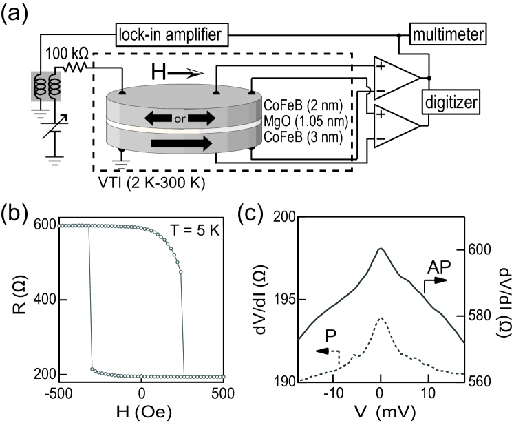
Figure 1: (a) Schematics of measurement setup and device structure. (b) Typical MR curves of the present MTJ measured at 5 K. (c) Typical differential resistance for P (dashed line) and AP (solid line) configurations as a function of bias voltage.

Resistance fluctuations are also important, as MTJs have found broad application, such as for magnetic field detectors, TMRapply1 magnetic random-access memory, TMRapply2 ; SekiAPL2011 random number generators SekiAPL2011 , and microwave oscillators. TMRapply3 For these applications, the signal-to-noise ratio is critically important, where the $1/f$ noise and RTN limit device performance at low frequency. There have been many reports of $1/f$ noise and RTN in MTJs with Al₂O₃-based, AlOnoise1 ; AlOnoise2 ; AlOnoise3 ; AlOnoise4 ; AlOnoise5 ; AlOnoise6 ; AlOnoise7 MgO-based, MgOnoise1 ; MgOnoise2 ; MgOnoise3 ; MgOnoise4 ; MgOnoise6 ; MgOnoise6_add ; MgOnoise7 ; MgOnoise8 ; MgOnoise9 ; MgOnoise9_add ; MgOnoise9_add2 ; MgOnoise10 ; MgOnoise11 and other tunneling barriers. Othernoise1 ; Othernoise2 Nevertheless, little is known about the noise properties of MTJs with submicron-sized junctions with a thin tunneling barrier, MgOnoise10 ; MgOnoise11 which are envisaged for memory and oscillator applications.

In this paper, we report on noise properties, including shot noise, $1/f$ noise, and RTN in well-crystalline MgO-based MTJs with submicron-sized junctions with thin tunneling barriers. The noise measurement was carried out at low temperature with high experimental accuracy, with a focus on the noise properties around the magnetic hysteresis loops of the free layer. We investigated each noise source systematically as a function of magnetic field and bias voltage. The clear dependence of the $1/f$ noise on the applied magnetic field indicates that the main origin of the $1/f$ noise is magnetic fluctuation in the free layer, which is discussed in terms of a fluctuation-dissipation relation. Based on the bias dependence of RTN, we discuss the origin of RTN, which is different from that of the $1/f$ noise. The analysis of shot noise is also presented to further support our previous report. MTJshot6

This paper is organized as follows: In Sec. IIA, we provide information on the sample fabrication and basic properties of our sample. Then the measurement system is described. In Sec. IIB, the analysis method to extract the frequency-dependent and frequency-independent components is explained. Section III is devoted to the experimental results and discussion. First, we show the magnetic field and bias-current dependence of frequency-dependent noise in Sec. IIIA, and then the origin of the $1/f$ noise is discussed by using the fluctuation-dissipation relation in Sec. IIIB. We estimate the fluctuating magnetic moment of the RTN in Sec. IIIC. The bias voltage dependence of the measured RTN is analyzed to obtain information on the excitation mechanism in Sec. IIID, and, finally, we show the result of the white noise component in Sec. IIIE. In Sec. IV, we conclude our study.

II Experiment

II.1 Device and measurement

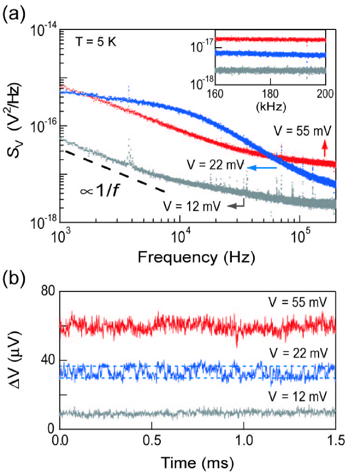
Figure 2: (a) Typical voltage noise spectral density of our MTJs in the AP configuration for different bias voltages: $V=12$, 22, and 55 mV at 5 K. The dashed line is a guide to the eye. The inset shows the same spectra between 160 and 200 kHz (but note that the bottom axis is a linear scale). (b) Measured real-time voltage fluctuations (with vertical offset for clarity) for the same condition as (a). The trace for $V=22$ mV contains two-level fluctuations, as indicated by the two horizontal dashed lines.

Multilayer stacks of MTJs were deposited in a magnetron sputtering system on a SiO₂ layer on a silicon substrate. The order of the layer structure from the substrate is as follows; buffer, PtMn(15), CoFe(2.5), Ru(0.85), CoFeB(3), MgO(1.05), CoFeB(2), and cap, where the top CoFeB layer serves as a free layer [see Fig. 1(a)]. The thickness of each layer is indicated in ($\ldots$) in nanometers. The multilayer stacks are patterned into elliptic pillars with $160\times 60$ nm dimensions by milling up to the middle of the PtMn layer. To crystallize CoFeB layers, the stack is annealed in $10,000$ Oe for 120 min at 330${\,}^{\circ}$C. TMR10 ; TMR11

All of the results presented here were obtained at low temperature (3–5 K) in the variable temperature insert (Oxford VTI) in a magnetic field ($H$) between $-40,000$ and 500 Oe. The schematic setup of our measurement system is shown in Fig. 1(a). A dc bias is applied under a constant current condition ($I$) by using the dc voltage source through a 100 k$\Omega$ resistor. The differential resistance ($dV/dI$) and the dc bias voltage ($V$) are measured by a lock-in amplifier and a digital multimeter, respectively. Figure 1(b) shows the typical MR curve around the hysteresis loop of the free layer at 5 K. The clear square shape of the curve without any steps indicates that there is no pinning site on a macroscopic domain wall. The MR ratio defined as $(R_{AP}-R_{P})/R_{P}$ is 208%, where $R_{P}$ and $R_{AP}$ are the sample resistances in the parallel (P) and antiparallel (AP) configurations, respectively. Figure 1(c) shows the typical bias dependence of the differential resistance, where the solid and dashed curves correspond to the AP ($-$500 Oe) and P (500 Oe) configurations, respectively. In the differential resistance, as temperature decreases below 10 K, a peak structure appears around the zero bias in both P and AP configurations, which is consistent with the several previous reports. TMR2 ; TMR3_add ; MTJshot2 Interestingly, in the P configuration, additional satellite peaks seem to appear around $V$ = $-$5 and 5 mV. Such a feature may be related to the observation reported before. TMRzero

To obtain the voltage noise spectral density $S_{V}$, we measure the time-domain voltage fluctuation signal by using a two-channel digitizer (National Instruments PCI-5922), which yields $S_{V}$ by a fast Fourier transformation. In this process, two sets of voltage signals are simultaneously measured after being independently amplified by two room-temperature amplifiers (NF Corporation LI-75A). The cross-correlation technique is used here to reduce the external noise and amplifier noise by long-time averaging. CrossCorr The frequency range of our system is 100 Hz to 200 kHz. In addition to $S_{V}$, the real-time voltage signal is also recorded by the digitizer at a sampling rate of 1 MHz.

The $S_{V}$ measurement is carefully calibrated with the thermal noise of several commercial resistors (MCY100R00T, MCY250R00T, MCY350R00T, and MCY1K0000T) with a precision of 0.01%. The typical resolution of $S_{V}$ for shot noise estimation is below $10^{-20}$ V${}^{2}/$Hz. As a result, we achieved an experimental precision for the Fano factor well below 1%. We measured three devices with the same geometry (samples 1, 2, and 3) which are made out of the single wafer, and obtained consistent results.

II.2 Analysis of noise

In the present experiment, we found that the voltage noises in MTJs consist of a white noise ($S_{\rm{white}}$), which is a frequency-independent component, $1/f$ noise ($S_{1/f}$), and RTN ($S_{\rm{RTN}}$): sum_add

$$S_{V}=S_{\rm{white}}+S_{1/f}+S_{\rm{RTN}}.$$ (1)

The white noise ($S_{\rm{white}}$) is attributed to the thermal agitation of electrons (thermal noise) and the partition process of electrons (shot noise). Then $S_{\rm{white}}$ is described by

$$S_{\rm{white}} = 4k_{B}TR_{d}$$ (2)

$$+ 2F\left[eIR_{d}^{2}\coth\left(\frac{eV}{2k_{B}T}\right)-2k_{B}TR_{d}\right],$$

where $k_{B}$ is Boltzmann’s constant, $e$ is the electron charge, $R_{d}$ is the differential resistance ($dV/dI$) at a given $V$ (or $I$), and $F$ is the Fano factor. The $1/f$ noise ($S_{1/f}$) in MTJs is parameterized by AlOnoise2

$$S_{1/f}=\frac{\alpha^{\ast}I^{2}R_{d}^{2}}{{A}f},$$ (3)

where $\alpha^{\ast}$, $f$, and $A$ are the Hooge parameter, frequency, and junction area, respectively. The RTN is the fluctuation between two levels, where $S_{\rm{RTN}}$ exhibits a Lorentzian character in an ideal case.

Typical results of $S_{V}$ for the AP configurations for $V=12$, 22, and 55 mV at 5 K are shown in Fig. 2(a). In the data, the resistor-capacitor (RC) damping owing to the capacitance (760 pF) of the measurement lines has already been corrected for. MTJshot6 In the inset of Fig. 2(a), which shows the region between 160 and 200 kHz, the spectra are almost flat, and thus the increase of $S_{V}$ with increasing $V$ corresponds to the shot noise. In contrast, the spectra for the low-frequency region strongly depend on the frequency, as shown in the main panel of Fig. 2(a). The spectra for $V=55$ and 12 mV are clearly dominated by the $1/f$ noise except for the high-frequency region. The spectrum for $V=22$ mV has a clear Lorentzian character, MgOnoise11 indicating that the source of the noise is two-level fluctuation of the resistance, namely, RTN. Figure 2(b) shows the real-time voltage signal for $V=12$, 22, and 55 mV. Apparently, the time-domain signal has a two-level nature only for $V=22$ mV, as indicated by the two horizontal dashed lines in Fig. 2(b).

We performed a histogram analysis between 160 and 200 kHz to estimate $S_{\rm{white}}$. MTJshot4 To investigate the $1/f$ noise and RTN, we first subtract the white noise component from the measured $S_{V}$ and then define the Hooge parameter $\alpha$ as

$$\alpha={A}\int_{f_{1}}^{f_{2}}\left(S_{V}-S_{\rm{white}}\right)df/I^{2}R_{d}^{2}\ln\left(\frac{f_{2}}{f_{1}}\right),$$ (4)

where the frequencies $f_{1}$ and $f_{2}$ are chosen to be 1 and 100 kHz, respectively. The value of $\alpha$ thus obtained equals the $\alpha^{\ast}$ in Eq. (3) when RTN is negligibly small. In this study, we mainly use the $\alpha$ that is a well-defined parameter even if RTN is present.

III Results and discussion

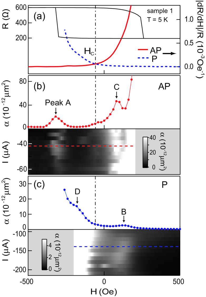
Figure 3: The magnetic field and bias current dependence of $\alpha$ measured at 5 K for sample 1. (a) MR curves of this MTJ and $|dR/dH|/R$ values for P (dashed line) and AP (solid line) configurations numerically estimated from the MR curves. The vertical dashed line marks $H=H_{c}$ at which $|dR/dH|/R$ for AP and P have the same value. (b) The measured $\alpha$ for AP (solid mark) configuration, where we marked the peaks of $\alpha$ as A and C (upper panel), and a color plot of $\alpha$ as a function of magnetic field and bias current (lower panel). The dashed line corresponds to $\alpha$ in the upper panel. (c) Counterpart of Fig. 3(b) for the P configuration, where the peaks of $\alpha$ are marked as B and D. $\alpha$ values for the two configurations were measured in almost the same bias voltage region.

III.1 Frequency-dependent noise

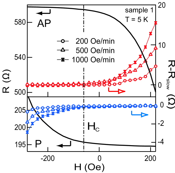
Figure 4: Field sweep rate dependence of dc resistance. The solid line is the dc resistance measured with the slowest sweep rate (50 Oe/min) as the field was ramped from $-500$ to 240 Oe for AP and 500 to $-300$ Oe for P. Results for other sweep rates (200, 500, and 1000 Oe/min) are plotted as differences from the slowest one.

We start with the experimental result of the frequency-dependent noise. There have been several studies on the field dependence of the $1/f$ noise in Al₂O₃-based AlOnoise1 ; AlOnoise2 ; AlOnoise3 ; AlOnoise4 ; AlOnoise5 ; AlOnoise7 and MgO-based MgOnoise1 ; MgOnoise2 ; MgOnoise3 ; MgOnoise6 ; MgOnoise6_add ; MgOnoise9 ; MgOnoise9_add ; MgOnoise9_add2 ; MgOnoise11 MTJs. In these reports, the measured $1/f$ noise consists of field-independent and field-dependent components. The former component has a nonmagnetic origin (charge trap in the tunneling barrier), whereas the latter component has a magnetic origin (magnetic fluctuations and domain wall motion in the free and/or fixed magnetic layers). Recent studies on the $1/f$ noise in MgO-based MTJs have shown that the nonmagnetic $1/f$ noise is no longer important owing to the improvement of tunneling barrier quality. MgOnoise9 For RTN, both magnetic and nonmagnetic origins were reported in Al₂O₃-based AlOnoise1 ; AlOnoise3 ; AlOnoise4 ; AlOnoise5 ; AlOnoise6 and MgO-based MgOnoise2 ; MgOnoise4 ; MgOnoise6 ; MgOnoise10 MTJs. Nevertheless, there are only a few systematic studies on the magnetic field and bias voltage dependence of RTN. Here we focus on the magnetic $1/f$ noise and RTN in the hysteresis loop of the free layer.

Figure 3(a) shows the resistance and $|dR/dH|/R$ at 5 K, which is obtained as the field is ramped from $-500$ to 200 Oe for AP and from 500 to $-240$ Oe for P configurations. The value of $\alpha$ measured at each field for AP and P configurations is shown in the upper panels of Figs. 3(b) and 3(c), respectively. It is clear that the magnetic field dependencies between $\alpha$ and $|dR/dH|/R$ resemble each other for the two configurations: MagLoss They increase with the reversal of the free layer, except for a few peaks observed in $\alpha$ [peaks A, B, C, and D in Figs. 3(b) and 3(c)]. Whereas the measured spectra are dominated by the $1/f$ noise outside of these peak regions, strong enhancement of Lorentzian character is always seen in such peak regions. The lower panels of Figs. 3(b) and 3(c) show image plots of $\alpha$ as a function of the magnetic field and the bias current for the AP and P configurations, respectively. In these figures, the ranges of the bias current for the two configurations are set to be almost the same with respect to the bias voltage. The curves shown in the upper panel of Figs. 3(b) and 3(c) correspond to the cross sections indicated by the dashed line in each image plot.

We define $H_{c}$ as the field at which $|dR/dH|/R$ gives the same value for the AP and P configurations [see Fig. 3(a)]. The behaviors of $\alpha$ and $|dR/dH|/R$ are found to be well symmetric with respect to $H_{c}$, except for the peaks. The values of $\alpha$ for AP and P configurations at their baselines are $3.3\times 10^{-12}$ and $2.7\times 10^{-13}$ $\mu$m², respectively. This subtle difference is presumably due to the magnetic fluctuation of the fixed layer. Remarkably, the peak positions are roughly symmetric with respect to $H_{c}$ (namely, peaks A and B, and peaks C and D). Finally, these symmetric behaviors with respect to $H_{c}$ are always observed on all three samples. We will discuss the implications of these observations later in Sec. IIID again.

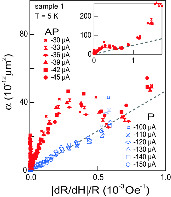
Figure 5: $\alpha$ at several bias currents vs $|dR/dH|/R$ for P (open symbols) and AP (solid symbols). The inset shows the full scale of the same data for AP. The dashed line is a guide to the eye.

The influence of the magnetic field sweep rate on the MR curve is shown in Fig. 4, where $H_{c}$ is also a relevant parameter. The resistance measured by each sweep rate is plotted as the difference of the data from that obtained with the slowest sweep rate (50 Oe/min), where the field was ramped from $-$500 to 240 Oe for AP and from 500 to $-$300 Oe for P configurations. Although initially there is no sweep rate dependence on the resistance for either configuration, a sweep rate dependence appears as the magnetic field crosses $H_{c}$. This observation strongly indicates that the free electrode feels zero effective field at $H_{c}$. The shift of $H_{c}$ from zero field is explained by taking a magnetic interaction between the free and fixed layers into account.

III.2 $1/f$ noise

Now, we discuss what we can learn from the $1/f$ noise. Previously, Ingvarsson et al. AlOnoise3 scaled $\alpha$ versus $|dR/dH|/R$ and explained the result in terms of a fluctuation-dissipation (FD) relation. The scaling of the $1/f$ noise by the FD relation has been tested against Al₂O₃-based AlOnoise3 ; AlOnoise4 and MgO-based MgOnoise9 ; MagLoss MTJs with micron-sized junction areas. Here, we test the scaling by the FD relation on the free layer of MgO-based MTJs with submicron-sized junctions following Ingvarsson et al. We replot the data in Figs. 3(c) and 3(d) and obtain the relation between $\alpha$ and $|dR/dH|/R$ as shown in Fig. 5. Remarkably, the values of $\alpha$ for the P configuration (open symbols) are almost proportional to $|dR/dH|/R$. For the AP configuration, the $\alpha$ values (solid symbols) first deviate from the dashed line (drawn to guide the eye) because of peaks A and C, and then fall onto the dashed line again. In the inset of Fig. 5, $\alpha$ for the AP configuration is shown over the wider range of $|dR/dH|/R$. After dropping onto the dashed line, $\alpha$ for AP rapidly increases with $|dR/dH|/R$ beyond $\sim$1 mOe^-1. In this region, the measured spectra exhibit a complicated enhancement of Lorentzian character possibly from several RTNs.

If one assumes thermal equilibrium, then the FD relation for this magnetic system is given by AlOnoise3

$$S_{m}=\frac{2k_{B}T}{\pi\mu_{0}f}\chi_{m}^{\prime\prime}\left(f\right),$$ (5)

where $S_{m}$, $\mu_{0}$, and $\chi_{m}^{\prime\prime}$ denote, respectively, the spectral density of magnetic fluctuation, the vacuum permeability, and the imaginary part of the magnetic susceptibility. Then by using a typical equation of $1/f$ noise [Eq. (3)] and the Kramers-Kronig relation, Eq. (5) reduces to AlOnoise3

$$\alpha^{\ast}=\frac{k_{B}T\textrm{A}\Delta R}{2m\mu_{0}R\ln\left(f_{max}/f_{min}\right)}\left(\frac{1}{R}\frac{dR}{dH}\right),$$ (6)

where 2$m$ and $\Delta R$ are the respective changes of the magnetic moment and resistance associated with the reversal of the free layer. Thus, the measured linear relation between $\alpha$ and $|dR/dH|/R$ for the P state in Fig. 5 can be explained by Eq. (6); namely, the origin of $1/f$ noise is thermal agitation of the magnetic moment of the free electrode. The dashed line corresponds to Eq. (6), where we take the saturation magnetization $M_{S}$ of CoFeB to be $1.3\times 10^{6}$ A/m. MgOnoise9 From rough estimation, we obtained $f_{max}/f_{min}\sim 10^{10\pm 2}$, which is consistent with the result $f_{max}/f_{min}\sim 10^{9}$ that Ingvarsson et al. AlOnoise3 reported. The nonlinear behavior with $|dR/dH|/R$ beyond $\sim$1 mOe^-1 is possibly caused by deviation from the thermal equilibrium state of the free layer. In fact, the measured dc resistance corresponding to this region strongly depends on the field sweep rate (see Fig. 4). According to previous works, MgOnoise9 ; MagLoss2 ; MagLoss3 the linear relation between $\alpha$ and $|dR/dH|/R$ corresponds to constant magnetic losses and has been shown by Stearrett et al. MagLoss in the P and AP configurations.

III.3 Random telegraph noise

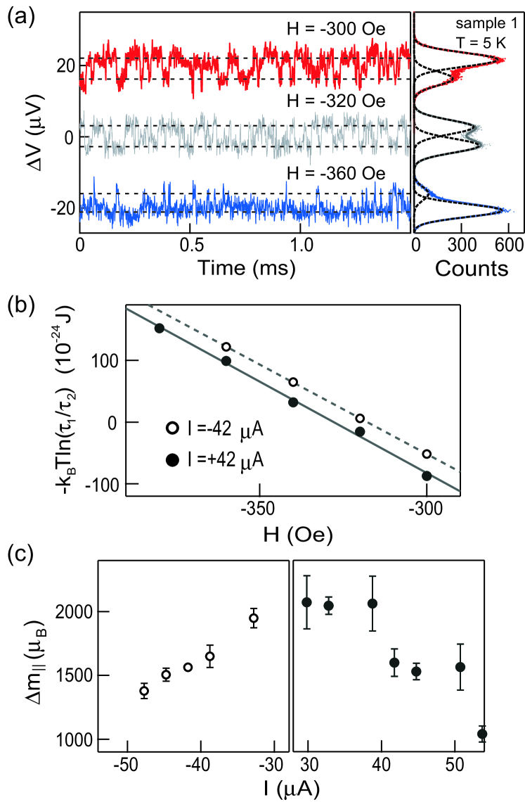
Figure 6: (a) Magnetic field dependence of the voltage fluctuations (offset for clarity) measured around peak A in Fig. 3(b) (left panel) and the corresponding histograms (dots) ($2\times 10^{5}$ points) (right panel). The solid and dashed curves are the fitted curves (double Gauss function) and each Gaussian component. (b) Logarithm of the rate of the dwell times for $I=-42$ $\mu$A (open circle) and 42 $\mu$A (solid circle) as a function of $H$. The dashed and solid lines are the results of the linear fitting. (c) Bias dependence of estimated fluctuation magnetic moments.

Previously magnetic RTN have been observed in Al₂O₃-based AlOnoise3 ; AlOnoise4 and MgO-based MgOnoise4 ; MgOnoise6 ; MgOnoise10 MTJs, which are typically sensitive to the magnetic field and bias voltage. Although it is difficult to deal with the RTN systematically in general, a few authors successfully estimated the effective magnetic moment of the fluctuator and discussed possible origins of magnetic RTN. In Al₂O₃-based MTJs with micron-sized junctions, Ingvarsson et al. AlOnoise3 and Jiang et al. AlOnoise4 suggested a small rotation of a single domain or domain wall hopping between pinning sites. Recently, Herranz et al. MgOnoise10 reported that the magnetic RTN is caused by magnetic inhomogeneities and domain walls in free and fixed layers.

We observed a strong enhancement of the Lorentzian components in regions with specific bias voltages and magnetic fields. Here we consider peaks A, B, C, and D in Fig. 3(b) as typical examples. Generally, the Lorentzian component in the noise spectral density indicates that the noise is caused by the fluctuation between two levels, namely, RTN. The real-time voltage signals near peak A for $H=-300$, $-$320, and $-$360 Oe are shown in the left panel of Fig. 6(a); the right panel shows the corresponding histograms for the voltage signals ($2\times 10^{5}$ points for 200 ms). These signals have two distinct voltage levels, and hence we attribute the measured Lorentzian components to RTN. The histograms are fitted by a double-Gaussian function, which is shown in the same panel by the dashed lines. Let us call the two states “1” and “2.” From the area of each Gaussian, which is proportional to the dwell time of each state ($\tau_{1}$ and $\tau_{2}$), we estimate the ratio of the dwell times between these states ($\tau_{1}/\tau_{2}$). Figure 6(b) shows a logarithmic plot of $\tau_{1}/\tau_{2}$ versus $H$ for $I=\pm 42$ $\mu$A. Remarkably, $\log\tau_{1}/\tau_{2}$ is proportional to the magnetic field. The strong dependence of the dwell time for each state as a function of magnetic field indicates that the RTN is due to a magnetic fluctuator.

We assume that two states with dwell times of $\tau_{1}$ and $\tau_{2}$ have activation energies of $E\pm\Delta\textbf{m}\cdot\textbf{H}$. By further assuming the Arrhenius relation, we express the dwell times $\tau_{1}$ and $\tau_{2}$ as

$$\frac{1}{\tau_{1,2}\left(H\right)}=\frac{1}{\tau_{0}}\exp\left(-\frac{E\pm\Delta\textbf{m}\cdot\textbf{H}}{k_{B}T}\right),$$ (7)

where $E$, $\Delta\textbf{m}$, and $1/\tau_{0}$ are the field-independent activation energy, the total magnetic moment of the fluctuator, and an attempt frequency, respectively (where we take + for the 1 state and $-$ for the 2 state). To estimate the effective magnetic moment parallel to $H$ ($\Delta m_{\parallel}$), we take the ratio of each dwell time: AlOnoise3 ; AlOnoise4 ; MgOnoise10 $\tau_{1}/\tau_{2}\propto\exp\left(-2\Delta m_{\parallel}H/k_{B}T\right)$. By a linear fit of $\ln\left(\tau_{1}/\tau_{2}\right)$ versus $H$ [see Fig. 6(b)], we estimated the effective magnetic moment $\Delta m_{\parallel}$ to be $1.6\times 10^{3}\mu_{B}$ for both positive and negative currents ($I=\pm 42$ $\mu$A), where $\mu_{B}$ is the Bohr magneton. This value corresponds to 0.08% of the total magnetic moment of the free electrode ($2.0\times 10^{6}\mu_{B}$). However, the change in resistance $\Delta R$ resulting from RTN was estimated from the real-time voltage signal to be 0.13 $\Omega$, which is about 0.035% of the total resistance change for the reversal of the free layer, which is consistent with the above value (0.08%). This observation strongly suggests that the observed RTN is responsible for the magnetic fluctuator. The bias dependence of the estimated $\Delta m_{\parallel}$ is shown in Fig. 6(c). With increasing bias current, $\Delta m_{\parallel}$ is monotonically decreased for both bias polarities. This means that as the injection current gets higher, smaller magnetic fluctuations are allowed.

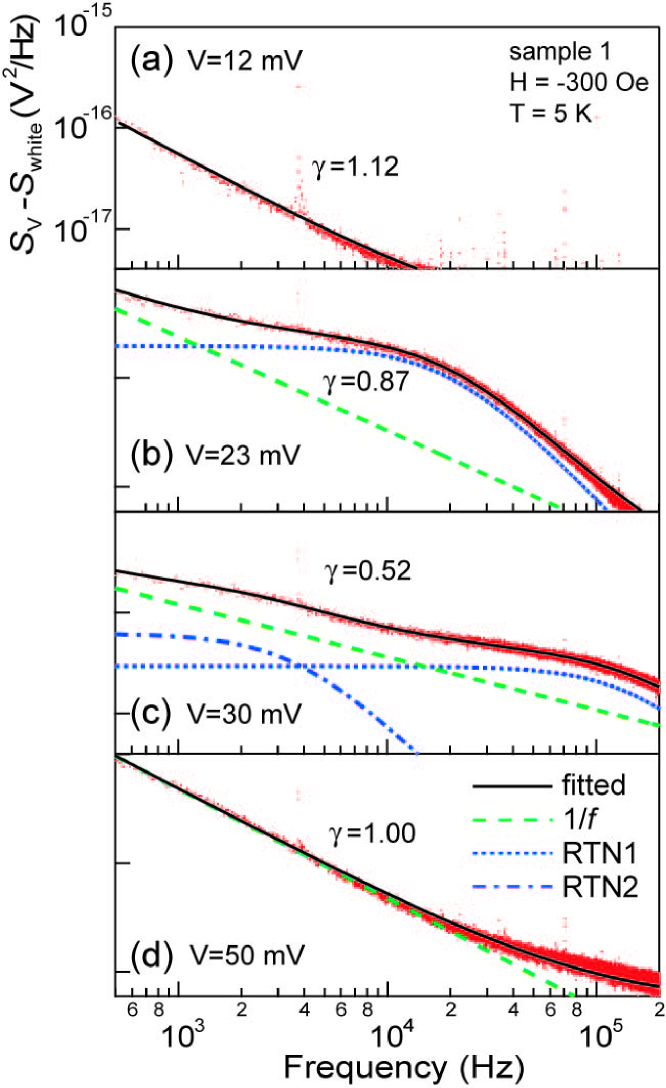
Figure 7: (a)–(d) The frequency-dependent component of the spectrum for $V=12$, 23, 30, and 50 mV, respectively. The solid curves are the fitted curves obtained by summing the $1/f$ noise, RTN1, and RTN2, where each component is shown as a dashed curve.

The $\Delta m_{\parallel}$ values in the previous reports AlOnoise3 ; AlOnoise4 ; MgOnoise10 are larger than those in our result by at least two orders of magnitude. Here we discuss the origin of the fluctuator that contributes to the measured magnetic RTN. If one assumes full reversal of a single domain in the free layer, a typical area size of the magnetic fluctuator is $5.9\times 10^{-6}\;\mu\text{m}^{2}$, where the junction area is $7.4\times 10^{-3}\;\mu\text{m}^{2}$. This small value and the absence of any step in the magnetic hysteresis loops in Fig. 4 indicate that the contribution of a macroscopic domain wall can be ruled out. The estimated $\Delta m_{\parallel}$ and $\Delta R$ for the AP configuration have almost the same percentages against the full reversal of the free layer. Finally, enhancement of magnetic RTN is observed for both configurations. Based on these results, we attribute the fluctuator to two quasistable single-domain states with some strain in the free layer. SekiAPL2011

III.4 Crossover from the $1/f$ noise to RTN

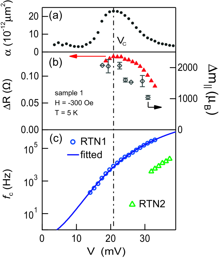
Figure 8: Bias dependence of the parameters characterizing the RTN at $-$300 Oe for AP. (a) Bias voltage dependence of $\alpha$. (b) The triangle is the resistance change of RTN1. The open diamond is the estimated fluctuating magnetic moments in Fig. 6(c). (c) $f_{c}$ for RTN1 (circle) and RTN2 (triangle). The solid curve is the fit to $f_{c}$ for RTN1

To understand the excitation mechanism of the RTN we focus on the bias dependence of the noise property at peak A. Figure 7 represents the frequency-dependent component of measured spectra at $-$300 Oe (AP configuration) for $V=12$, 23, 30, and 50 mV. Although pure $1/f$ noise is observed in the low-bias region as shown in Fig. 7(a), RTN is dominant at $V=23$ mV, resulting in the strong enhancement of the Lorentzian component (“RTN1”) [Fig. 7(b)]. The characteristic frequency of the RTN is given by the full width at half maximum of the Lorentzian ($f_{c}$). For example, $f_{c}=20$ kHz for RTN1 in Fig. 7(b). With increasing bias voltage, the characteristic frequency of RTN1 increases and another Lorentzian component (“RTN2”) with different $f_{c}$ appears [Fig. 7(c)]. Finally, the $1/f$ noise becomes dominant again in the spectrum [Fig. 7(d)]. To fit the obtained spectra as a summation of $1/f$ noise ($S_{\rm{1/f}}$) and a few Lorentzians ($S_{\rm{RTNi}}$), we use $\beta/f^{\gamma}$ and $\beta_{i}^{\ast}/[1+(f/f_{ci})^{2}]$, respectively. Here $\gamma$ and $f_{ci}$ are the spectral exponent and characteristic frequency of the Lorentzian for “RTN$i$” ($i=1$ and 2). Outside the peak region, the estimated $\gamma$ is close to 1, whereas it is reduced from 1 as the Lorentzian components are enhanced. By taking the Dutta-Dimon-Horn model, Dutta in which the $1/f$ noise is the result of a superposition of many RTNs with a broad distribution of activation energies, this suppression of $\gamma$ accompanied by the enhancement of RTN can be explained by a change of the energy distribution of the magnetic fluctuators.

The bias dependence of the parameters characterizing RTN at $-300$ Oe for the AP configuration is summarized in Fig. 8. $V_{c}\sim 21$ mV is the bias voltage where $\alpha$ shows its maximum. The effective magnetic moment of the fluctuator, $\Delta m_{\parallel}$, and the change in resistance, $\Delta R$, are compared in Fig. 8(b). The behaviors of $\alpha$, $\Delta m_{\parallel}$, and $\Delta R$ are similar to each other in that they have their maxima at $V_{c}$ and then decrease as the bias is increased. Finally, both $\Delta m_{\parallel}$ and $\Delta R$ become almost half of their maxima at the bias at which the peak of $\alpha$ disappears. Figure 8(c) shows that, although the estimated $f_{c}$ for RTN1 and RTN2 exhibits almost an exponential increase with the bias for their whole curves, there is a kneelike structure in the curve for RTN1 at $V_{c}$. We fit $f_{c}$ for RTN1 to $f_{c}=f_{0}\exp\left(-E/k_{B}T^{\ast}\right)$ using the Arrhenius relation and taking Joule heating into account, where $f_{0}$ is an attempt frequency. We also assume that the activation energy $E$ is independent of the bias voltage and that the effective temperature $T^{\ast}=T+\zeta V^{2}$. The solid curve in Fig. 8(c) corresponds to the fitted curve, where the estimated $E$ and $\zeta$ are $1.3\times 10^{-21}\text{ J}$ and $1.3\times 10^{4}\text{ K}/\text{V}^{2}$, respectively. Comparing this result to the previous one, AlOnoise6 in which the activation energy for nonmagnetic RTN in Al₂O₃-based MTJs was found to be $0.3\times 10^{-19}\text{ J}$, we see that our value is much smaller. This is consistent with the absence of nonmagnetic RTN in high-quality MTJs in the low-temperature, low-bias regime.

Returning to the magnetic configuration dependence of the RTN, one sees that $\alpha$ values for peaks A and B are enhanced at roughly symmetric positions with respect to $H_{c}$ [see lower panels in Figs. 3(b) and 3(c)]. The values of $\alpha$ for peaks A and B have their maxima at almost the same bias voltage, whereas the amplitude of the maximum for peak A is almost seven times as large as that of peak B. We assume that the same magnetic fluctuator contributes to these two peaks. The symmetric hysteresis loop of the free layer with respect to $H_{c}$ also supports this assumption (see Fig. 4). Here, the difference in the peak amplitude between A and B cannot be accounted for by conventional Joule heating. That is, because the Joule heating effect is proportional to the bias current at a fixed bias voltage, this effect for peak A is only 1/3 that for peak B. These results may imply a spin-dependent heating process of a localized spin system in the free layer depending on the magnetic configurations.

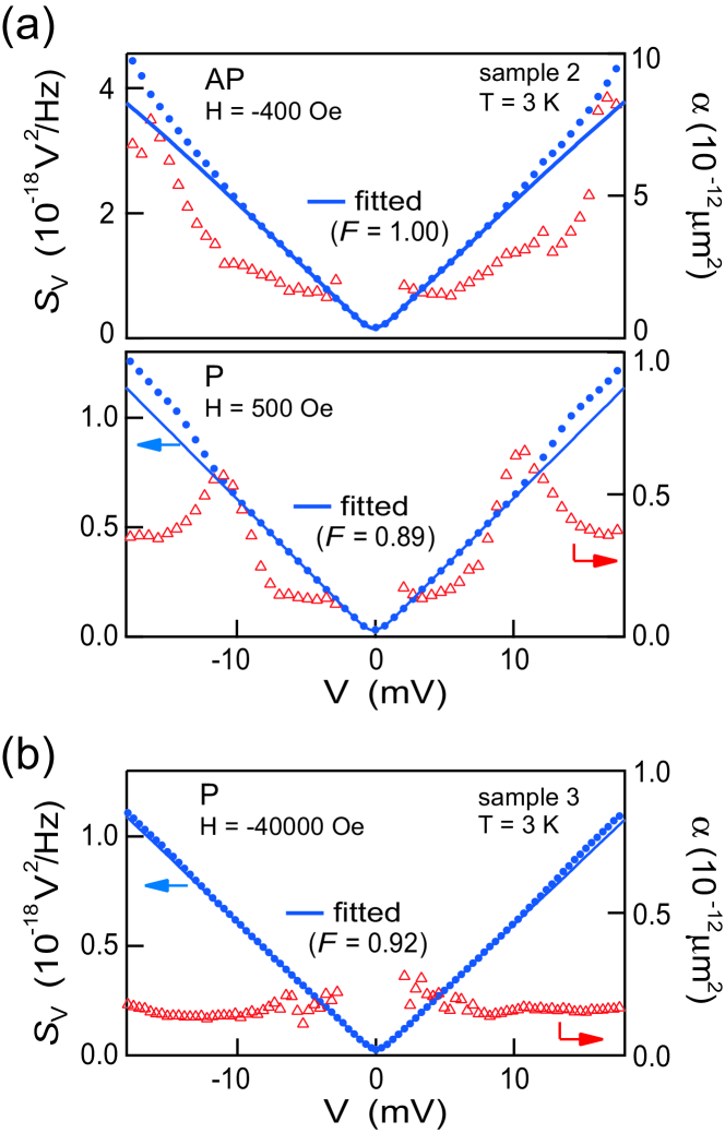
Figure 9: (a) White noise component and $\alpha$ measured at 3 K in the P ($H=500$ Oe) and AP ($H=-400$ Oe) configurations on sample 2 as a function of $V$. The solid curve is the fitted curve between $V=-10$ and 10 mV. (b) Counterpart of Fig. 9(a) in the P configuration ($H=-40,000$ Oe) on sample 3.

III.5 Shot noise

Finally, we discuss the shot noise to connect our previous work with the present one and to support further evidence of our claim made before. The frequency-independent component of the spectrum is well described by Eq. (1). $F$ describes how the noise deviates from the Poissonian value and thus characterizes the partition process of the electron tunneling. Conventional tunnel junctions exhibit $F=1$, reflecting the Poissonian process. Regarding Al₂O₃-based MTJs, after the first report of the full shot noise ($F\sim 1$), AlOnoise4 reduced Fano factors ranging from 0.45 to 1 were reported. MTJshot1 ; MTJshot2 This reduction can be explained by the sequential tunneling model, MTJshot2 where the process of two-step tunneling through impurities within the barrier is assumed. In this theoretical model, $F$ strongly depends on the asymmetry of the each tunneling and can be 0.5 to 1.

Full shot noise in MgO-based MTJs was reported by Guerrero et al. and some of the authors of the present paper in experiments where the MgO barriers were as thick as 3 and 1.5 nm, respectively. MTJshot3 ; MTJshot4 This indicates that MgO-based MTJs are free from the process through impurity sites, possibly resulting from the high quality of the crystallized MgO. Later, we reported the suppression of the Fano factor for the P configuration (typically 0.91) with a 1.05-nm-thick MgO barrier, whereas the $F$ for the AP configuration is almost unitary (typically 0.99). MTJshot6 To explain this subtle reduction of $F$ within the above sequential tunneling model, we have to assume a very asymmetric barrier (1:100), which is unrealistic as the barrier of our MTJ is thin. Moreover, by using this model, we cannot explain the magnetic configuration dependence of the reduced $F$, and hence we can rule out this scenario. We note that all of the experimental results for $F$ values including the thick-barrier case can be explained by recent theoretical work based on a first-principles calculation. MTJshot7 Namely, the Fano factor, which is reduced from 1, is a direct consequence of the Pauli exclusion principle, signaling that there are coherent channels with high transmission probabilities through the epitaxial MgO barriers. Thus, our result on the shot noise gives unique evidence for coherent tunneling through a crystallized MgO barrier.

We show in Fig. 9 the typical results of the white-noise component $S_{V}$ and $\alpha$ at 3 K as a function of bias voltage. In Fig. 9(a), $S_{V}$ is nicely fitted by Eq. (2) for $|V|\leq 10$ mV. For $|V|>10$ mV, $\alpha$ increases due to enhancement of RTN for both configurations, and, as a result, $S_{V}$ deviates from the fitted curve. It is noted that the effect of the $1/f$ noise on $S_{V}$ is negligibly small in this bias range. The above observation indicates that to accurately estimate the Fano factor immune to the frequency-dependent noise, it is necessary to analyze the noise in the low-bias regime at low temperature. Experimentally, we can suppress magnetic RTN by stabilizing the magnetization by applying a large magnetic field for the P configuration. In fact, in Fig. 9(b), the enhancement of RTN is suppressed, and thus $S_{V}$ is almost perfectly fitted by the shot-noise formula with $F=0.92$.

IV Conclusion

The low-frequency noise properties in submicron-sized CoFeB/MgO/CoFeB-based MTJs with thin tunneling barriers are systematically investigated. The measurements are carried out at low temperature by controlling the magnetic field and bias current (voltage), where we focus on the noise properties on the magnetic hysteresis loops of the free layer. A clear correlation between $\alpha$ and $|dR/dH|/R$ is observed. The nice scaling of the observation by the FD relation indicates that the main origin for the $1/f$ noise is thermal magnetic fluctuation of the free layer. RTN is observed inside the magnetic hysteresis loops for both configurations. We found that this is due to the magnetic fluctuation between two quasistable single-domain states with some strain in the free layer. Although the $1/f$ noise is almost independent of the magnetic configuration, RTN is remarkably enhanced for the AP configuration and at specific bias voltages. Such results indicate a spin-dependent activation process of RTN. Shot noise measurement gives us quantitative information for coherent tunneling.

Our study shows that a systematic study on the noise of MTJs is possible by using devices with well-crystallized thin MgO barriers and by measuring the noise at low temperature and low bias. Further study of the noise properties in MgO-based MTJs with various barrier thicknesses is necessary to systematically elucidate the mechanism of the noise and improve the device properties.

References

- (1) S. Yuasa, J. Phys. Soc. Jpn. 77, 031001 (2008).
- (2) M. Julliere, Phys. Lett. A 54, 225 (1975).
- (3) T. Miyazaki and N. Tezuka, J. Magn. Magn. Mater. 139, L231 (1995).
- (4) J. S. Moodera, L. R. Kinder, T. M. Wong, and R. Meservey, Phys. Rev. Lett. 74, 3273 (1995).
- (5) S. Yuasa, T. Nagahama, A. Fukushima, Y. Suzuki, and K. Ando, Nature Mater. 3, 868 (2004).
- (6) S. S. P. Parkin, C. Kaiser, A. Panchula, P. M. Rice, B. Hughes, M. Samant, and S. H. Yang, Nature Mater. 3, 862 (2004).
- (7) W. H. Butler, X.-G. Zhang, T. C. Schulthess, and J. M. MacLaren, Phys. Rev. B 63, 054416 (2001).
- (8) J. Mathon and A. Umerski, Phys. Rev. B 63, 220403R (2001).
- (9) X.-G. Zhang and W. H. Butler, Phys. Rev. B 70, 172407 (2004).
- (10) R. Landauer, Nature (London) 392, 659 (1998).
- (11) Ya. M. Blanter and M. Büttiker, Phys. Rep. 336, 1 (2000).
- (12) L. Spietz, K. W. Lehnert, I. Siddiqi, and R. J. Schoelkopf, Science 300, 1929 (2003).
- (13) S. Yuasa, T. Nagahama, and Y. Suzuki, Science 297, 234 (2002).
- (14) T. Nagahama, S. Yuasa, E. Tamura, and Y. Suzuki, Phys. Rev. Lett. 95, 086602 (2005).
- (15) L. Jiang, J. F. Skovholt, E. R. Nowak, and J. M. Slaughter, Proc. SPIE 5469, 13 (2004).
- (16) R. Guerrero, F. G. Aliev, Y. Tserkovnyak, T. S. Santos, and J. S. Moodera, Phys. Rev. Lett. 97, 266602 (2006).
- (17) R. Guerrero, D. Herranz, F. G. Aliev, F. Greullet, C. Tiusan, M. Hehn, and F. Montaigne, Appl. Phys. Lett. 91, 132504 (2007).
- (18) K. Sekiguchi, T. Arakawa, Y. Yamauchi, K. Chida, M. Yamada, H. Takahashi, D. Chiba, K. Kobayashi, and T. Ono, Appl. Phys. Lett. 96, 252504 (2010).
- (19) A. Gokce, R. Stearrett, E. R. Nowak, C. Nordman, Fluctuation Noise Lett. 10, 381 (2011)
- (20) T. Arakawa, K. Sekiguchi, S. Nakamura, K. Chida, Y. Nishihara, D. Chiba, K. Kobayashi, A. Fukushima, S. Yuasa, and T. Ono, Appl. Phys. Lett. 98, 202103 (2011).
- (21) J. P. Cascales, D. Herranz, F. G. Aliev, T. Szczepański, V. K. Dugaev, J. Barnaś, A. Duluard, M. Hehn, and C. Tiusan, Phys. Rev. Lett. 109, 066601 (2012).
- (22) T. Tanaka, T. Arakawa, K. Chida, Y. Nishihara, D. Chiba, K. Kobayashi, T. Ono, H. Sukegawa, S. Kasai, and S. Mitani, Appl. Phys. Express 5, 053003 (2012).
- (23) K. Liu, K. Xia, and G. E. W. Bauer, Phys. Rev. B 86, 020408R (2012).
- (24) R. C. Chaves, P. P. Freitas, B. Ocker, and W. Maass, Appl. Phys. Lett. 91, 102504 (2007).
- (25) Z. M. Zeng, P. K. Amiri, G. Rowlands, H. Zhao, I. N. Krivorotov, J.-P. Wang, J. A. Katine, J. Langer, K. L. Wang, and H. W. Jiang, Appl. Phys. Lett. 98, 072512 (2011).
- (26) T. Seki, A. Fukushima, H. Kubota, K. Yakushiji, S. Yuasa, and K. Ando, Appl. Phys. Lett. 99, 112504 (2011).
- (27) D. Houssameddine, S. H. Florez, J. A. Katine, J.-P. Michel, U. Ebels, D. Mauri, O. Ozatay, B. Delaet, B. Viala, L. Folks, B. D. Terris, and M.-C. Cyrille, Appl. Phys. Lett. 93, 022505 (2008).
- (28) E. R. Nowak, R. D. Merithew, M. B. Weissman, I. Bloom, and S. S. P. Parkin, J. Appl. Phys. 84, 6195 (1998).
- (29) E. R. Nowak, M. B. Weissman, and S. S. P. Parkin, Appl. Phys. Lett. 74, 600 (1999).
- (30) S. Ingvarsson, G. Xiao, S. S. P. Parkin, W. J. Gallagher, G. Grinstein, and R. H. Koch, Phys. Rev. Lett. 85, 3289 (2000).
- (31) L. Jiang, E. R. Nowak, P. E. Scott, J. Johnson, J. M. Slaughter, J. J. Sun, and R. W. Dave, Phys. Rev. B 69, 054407 (2004).
- (32) P. Dhagat, A. Jander, and C. A. Nordman, J. Appl. Phys. 97, 10C911 (2005).
- (33) F. Liu, Y. Ding, R. Kemshetti, K. Davies, P. Rana, and S. Mao, J. Appl. Phys. 105, 07C927 (2009).
- (34) F. Guo, G. McKusky, and E. D. Dahlberg, Appl. Phys. Lett. 95, 062512 (2009).
- (35) R. Guerrero, F. G. Aliev, R. Villar, J. Hauch, M. Fraune, G. Gunterodt, K. Rott, H. Bruckl, and G. Reiss, Appl. Phys. Lett. 87, 042501 (2005).
- (36) A. F. M. Nor, T. Kato, S. J. Ahn, T. Daibou, K. Ono, M. Oogane, Y. Ando, and T. Miyazaki, J. Appl. Phys. 99, 08T306 (2006).
- (37) A. Gokce, E. R. Nowak, S. H. Yang, and S. S. P. Parkin, J. Appl. Phys. 99, 08A906 (2006).
- (38) J. Scola, H. Polovy, C. Fermon, M. Pannetier-Lecoeur, G. Feng, K. Fahy, and J. M. D. Coey, Appl. Phys. Lett. 90, 252501 (2007).
- (39) D. Mazumdar, X. Liu, B. D. Schrag, M. Carter, W. Shen, and G. Xiao, Appl. Phys. Lett. 91, 033507 (2007).
- (40) F. G. Aliev, R. Guerrero, D. Herranz, R. Villar, F. Greullet, C. Tiusan, and M. Hehn, Appl. Phys. Lett. 91, 232504 (2007).
- (41) R. Guerrero, M. Pannetier-Lecoeur, C. Fermon, S. Cardoso, R. Ferreira, and P. P. Freitas, J. Appl. Phys. 105, 113922 (2009).
- (42) Z. Diao, J. F. Feng, H. Kurt, G. Feng, and J. M. D. Coey, Appl. Phys. Lett. 96, 202506 (2010).
- (43) R. Stearrett, W. G. Wang, L. R. Shah, J. Q. Xiao, and E. R. Nowak, Appl. Phys. Lett. 97, 243502 (2010).
- (44) R. Stearrett, W. G. Wang, L. R. Shah, A. Gokce, J. Q. Xiao, and E. R. Nowak, J. Appl. Phys. 107, 064502 (2010).
- (45) G. Q. Yu, Z. Diao, J. F. Feng, H. Kurt, X. F. Han, and J. M. D. Coey, Appl. Phys. Lett. 98, 112504 (2011).
- (46) D. Herranz, A. Gomez-Ibarlucea, M. Schäfers, A. Lara, G. Reiss, and F. G. Aliev, Appl. Phys. Lett. 99, 062511 (2011).
- (47) B. Zhong, Y. Chen, S. Garzon, T. M. Crawford, and R. A. Webb, J. Appl. Phys. 109, 07C725 (2011).
- (48) R. Guerrero, A. Solignac, C. Fermon, M. Pannetier-Lecoeur, Ph. Lecoeur, and P. Fernández-Pacheco, Appl. Phys. Lett. 100, 142402 (2012).
- (49) D. D. Djayaprawira, K. Tsunekawa, M. Nagai, H. Maehara, S. Yuasa, Y. Suzuki, and K. Ando, Appl. Phys. Lett. 86, 092502 (2005).
- (50) S. Yuasa, Y. Suzuki, T. Katayama, and K. Ando, Appl. Phys. Lett. 87, 242503 (2005).
- (51) J. M. Teixeira, J. Ventura, J. P. Araujo, J. B. Sousa, P. Wisniowski, S. Cardoso, and P. P. Freitas, Phys. Rev. Lett. 106, 196601 (2011).
- (52) M. Sampietro, L. Fasoli, and G. Ferrari, Rev. Sci. Instrum. 70, 2520 (1999).
- (53) W. F. Egelhoff Jr., P. W. T. Pong, J. Unguris, R. D. McMichael, E. R. Nowak, A. S. Edelstein, J. E. Burnette, and G. A. Fischer, Sens. Actuators A 155, 217 (2009).
- (54) R. Stearrett, W. G. Wang, X. Kou, J. F. Feng, J. M. D. Coey, J. Q. Xiao, and E. R. Nowak, Phys. Rev. B 86, 014415 (2012).
- (55) N. Smith, A. M. Zeltser, D. L. Yang, and P. V. Koeppe, IEEE Trans. Magn. 33, 3385 (1997).
- (56) A. Ozbay, A. Gokce, T. Flanagan, R. A. Stearrett, E. R. Nowak, and C. Nordman, Appl. Phys. Lett. 94, 202506 (2009).
- (57) P. Dutta, P. Dimon, and P. M. Horn, Phys. Rev. Lett. 43, 646 (1979).