The role of viscoelastic contrast in orientation selection of block copolymer lamellar phases under oscillatory shear

Abstract

The mesoscale rheology of a lamellar phase of a block copolymer is modeled as a structured fluid of uniaxial symmetry. The model predicts a viscoelastic response that depends on the angle between the the local lamellar planes and velocity gradients. We focus on the stability under oscillatory shear of a two layer configuration comprising a parallel and a perpendicularly oriented domain, so that the two layers have a different viscoelastic modulus $G^{*}(\omega)$. A long wave, low Reynolds number expansion is introduced to analytically obtain the region of stability. When the response of the two layers is purely viscous, we recover earlier results according to which the interface is unstable for non zero Reynolds number flows when the thinner layer is more viscous. On the other hand, when viscoelasticity is included, we find that the interface can become unstable even for zero Reynolds number. The interfacial instability is argued to dynamically favor perpendicular relative to parallel orientation, and hence we suggest that the perpendicular orientation would be selected in a multi domain configuration in the range of frequency $\omega$ in which viscoelastic contrast among orientations is appreciable.

I Introduction

A stability analysis of two superposed fluid layers to oscillatory shear is given when the frequency dependent viscoelastic modulus of each layer is different. At vanishing Reynolds number, we find that an initially planar interface can be rendered linearly unstable to long wavelength perturbations by viscoelastic contrast. Our analysis is motivated by rheology and alignment studies of structured phases, mostly in soft and biological matter, in which local viscoelastic response couples to a broken symmetry variable of the phase (e.g., orientation). The specific case considered is related to alignment studies of lamellar phases in bulk block copolymer melts. There by reason of symmetry, the complex viscoelastic modulus $G^{*}(\omega)$ depends on the relative orientation between local lamellar normal and velocity gradient. We argue that given the dependence of $G^{*}(\omega)$ on orientation, the hydrodynamic instability discussed here would dynamically favor domains of perpendicular orientation over parallel in a bulk, multi domain configuration.

Block copolymers are currently being investigated for a wide variety of applications in nanotechnology park03 ; re:black05 ; re:zschech07 ; tang08 ; re:pujari12 ; re:xie13 due to their ability to self-assemble into ordered nanophases of different symmetry (lamellar, cylindrical, spherical, close packed spherical, or bi-continuous phases such as gyroid). re:yamada04 ; re:guo08 ; re:lee10 Equilibrium morphologies and characteristic length scales can be easily controlled by chemical manipulation of the polymer blocks. In general, however, quenched block copolymer samples are macroscopically disordered in that they contain a large number of domains of different orientation, all degenerate by symmetry. Given that disordered or defected samples are not generally suitable for applications re:harrison00b ; re:kim03 ; re:kramer05 ; re:bosworth07 , a number of strategies have been put forward to accelerate annealing of defects, or to post process polycrystalline samples in order to increase the characteristic size of ordered domains. Applied shears have been particularly effective in aligning thin films of in-plane cylinder re:angelescu04 , sphere forming re:angelescu05 , and lamellar re:pujari12 phases. The same strategy has been used on bulk samples re:zhang95b ; re:patel95 ; chen98 ; wu05 , although there is no explanation yet as to the selected orientation relative to the shear as a function of material parameters, and amplitude and frequency of the shear wu05 . This lack of understanding of the non equilibrium processes involved in the alignment of bulk samples has led to alternative strategies including, for example, solvent annealing and applied electric fields re:olszowka09 .

Our current understanding of shear alignment in bulk samples is well summarized by Wu et al. wu05 . They conducted a systematic analysis in styrene-isoprene (SI) multiblocks (from diblocks to undecablocks). Results for diblocks confirm earlier experimental findings that show a sequence of transitions from parallel orientation at low frequencies, to perpendicular, and again to parallel as the frequency is increased. The sequence of transitions is qualitatively different in poly-(ethylene-propylene) - poly-(ethylethylene) (PEP-PEE) diblocks, presumably because a marked viscoelastic contrast between styrene and isoprene blocks which is largely absent in PEP-PEE. This issue was already emphasized by Fredrickson re:fredrickson96 who noted that styrene is largely unentangled, whereas isoprene is entangled, and hence a large contrast in relaxation times of the blocks is anticipated. Further, the experiments of Wu et al.wu05 show that this double transition is observed in diblocks and triblocks, but surprisingly not in higher order multiblocks, in which entanglement effects among longer chains would be expected to be more important.

A further complicating factor in the elucidation of the orientation selected under shear is the non terminal viscoelastic response of the block copolymer melt in the range of frequencies in which orientation switching is observed. koppi92 ; larson93 ; gupta95 ; wu05 (terminal behavior has an elastic modulus that vanishes with frequency as $G^{\prime}\sim\omega^{2}$ whereas the loss modulus reflects Newtonian viscous dissipation $G^{\prime\prime}\sim\omega$). In fact, non terminal rheology is observed even at the lowest frequencies at which $G^{*}(\omega)$ has been measured, a range well below that which can be attributed to individual chain dynamics.rosedale90 Interestingly, a dependence of the non terminal viscoelasticity on lamellar orientation has also been found in largely oriented samples. koppi92 ; larson93 ; gupta95 ; wu05 Except for diblocks, all multiblocks in Ref. wu05, show terminal behavior as $\omega\rightarrow 0$ when aligned along the perpendicular orientation, whereas none of them are terminal in the parallel orientation. This observation, together with the prominent entanglement effects described above, calls into question existing theoretical analyses that either neglect hydrodynamics or, if they don’t, they assume Newtonian flows. Viscoelastic response appears to be closely correlated with orientation, and is certainly not negligible even at the lowest frequencies probed.

We propose a new viscoelastic model of block copolymer melts that explicitly takes into account the fact that the melt in a lamellar phase is a uniaxial (not isotropic) fluid. As such, local viscoelastic response involves the coupling between local orientation of the lamellae and local strain and velocity gradients. For an incompressible system, such a symmetry requires three viscosity coefficients and three elastic moduli re:martin72 . We extend here the earlier analysis of a purely viscous uniaxial fluid huang07 , to incorporate viscoelasticity. As shown below, a uniaxial viscoelastic medium readily allows for differential rheology in, say, parallel and perpendicular orientations, including the observed terminal behavior of the perpendicular orientation versus viscoelastic response of other orientations.

For simplicity, our analysis does not address a macroscopically disordered sample, but rather a configuration comprising only two perfectly oriented domains and the boundary separating them. Of the three possible orientations of an ordered lamellar domain relative to the imposed shear we focus here on parallel and perpendicular only. The third independent component (the so called transverse, in which the lamellar normal is parallel to the velocity direction), is less stable as it is being compressed by the shear re:chen02 . Both parallel and perpendicularly oriented domains are marginal with respect to the flow, and as such have been the subject of most orientation selection studies to date.

Section II describes the model equations and the fluid configuration under consideration. We introduce a general linear viscoelastic constitutive law for a incompressible system with uniaxial symmetry, and derive the reference flow under oscillatory shear and a planar boundary separating two layers of different orientation. Section III presents our results concerning the linear instability of the base state by considering small perturbations of large wavelength, also in the limit of small Reynolds number. The implications of our findings on orientation selection in a lamellar block copolymer are discussed in Sec. IV.

II Viscoelastic mesoscopic model

Although the description below can be generalized to the case of a multi block (see, e.g., Ref. re:xie13, ), we start by introducing the two fluid model of a diblock copolymer for monomers of type A and B. At sufficiently low frequencies so that the individual polymer chains have relaxed to their equilibrium conformation, the state of the copolymer can be described by a local order parameter $\psi\sim\rho_{\text{A}}-\rho_{B}$, where $\rho_{A}$ and $\rho_{B}$ are the number fractions of monomers A and B respectively. The evolution of the order parameter has a relaxational component that is driven by free energy reduction re:fredrickson94 If fluid flow is allowed, there is a reversible contribution to the order parameter equation that incorporates advection by the local flow. If $v_{i}$ is the $i-th$ component of the local fluid velocity, the advection term for an incompressible fluid is $v_{i}\partial_{i}\psi$, where sum over repeated indices is assumed. The flow velocity $v_{i}$ satisfies the momentum conservation equation with the stress tensor being the momentum density current. We now introduce a general linear constitutive law for the stress tensor of the form,

$$\sigma_{ij}=\int_{-\infty}^{t}dt^{\prime}\;G_{ijkl}(t-t^{\prime})\Big{[}\partial_{k}v_{l}(t^{\prime})+\partial_{l}v_{k}(t^{\prime})\Big{]}.$$ (1)

The independent contributions to a fourth rank tensor compatible with incompressible condition ($\delta_{ij}\partial_{i}v_{j}=0$) and uniaxial symmetry ($\hat{q}_{i}$ is the $i-th$ component of the local unit normal to the lamellar planes, and assume that the constitutive law is invariant under $\hat{q}_{i}\rightarrow-\hat{q}_{i}$) can be written as

$$\begin{split}G_{ijkl}(t)=&G_{1}(t)\hat{q}_{i}\hat{q}_{j}\hat{q}_{k}\hat{q}_{l}+G_{4}(t)(\delta_{ik}\delta_{jl}+\delta_{il}\delta_{jk})\\ &+G_{56}(t)\Big{[}\hat{q}_{i}(\hat{q}_{k}\delta_{jl}+\hat{q}_{l}\delta_{kj})+\hat{q}_{j}(\hat{q}_{k}\delta_{il}+\hat{q}_{l}\delta_{ki})\Big{]},\end{split}$$ (2)

where $\delta_{ij}$ is the Kronecker’s delta. There are, in this case, three independent modulus components $G_{1},G_{4}$ and $G_{56}$ and, as a consequence, the viscoelastic response depends on the local lamellar orientation. For example, for perfect parallel lamellae ($\hat{\bf q}\parallel\nabla v$) $G_{\parallel}(t)=G_{4}(t)+G_{56}(t)$, and for perfect perpendicular lamellae ($\hat{\bf q}\parallel\nabla\times{\bf v}$) $G_{\perp}(t)=G_{4}(t)$. Therefore, any viscoelastic contrast between these two orientations is contained in the component $G_{56}(t)$. Note, in particular, that if the response of the material in the parallel configuration is terminal, this has to be the case for a perpendicular orientation as well. The reverse, however, is not true, fact that is consistent with experiments wu05 .

We focus here on extending the results of Ref. huang07, to include uniaxial viscoelasticity. We consider two semi infinite layers of a lamellar block copolymer, one on top of the other (Fig. 1), confined between two infinite and parallel planes. The phase at the top has thickness $H$, and the lower phase $h$. The upper plane oscillates with a velocity ${\bf U}$ of frequency $\omega$ and amplitude $U$ while the lower plane is at rest. The densities of two layers, $\rho$, are constant and equal since they are the same copolymer, differing only on lamellar orientation. For simplicity, we neglect any variation in the vorticity direction ($\nabla\times{\bf U}$), or $\hat{y}$ in Fig. 1. Hence we focus on a two dimensional system in which the fluid velocity has components $v_{i}^{(\alpha)}=(u^{(\alpha)},0,w^{(\alpha)})$ with $\alpha=1,2$ denoting fluid 1 (lower) or 2 (upper).

When the two layers in this configuration contain parallel and perpendicular phases, the state of the system is unaffected by the flow since ${\mathbf{v}}\cdot\nabla\psi=0$ for both orientations. Furthermore, if as is customary, both phases are assumed to be isotropic fluids, then the configuration shown is stable, the order parameter is stationary, and the flow is a simple linear shear. If, on the other hand, Eq. (2) is assumed, then the two layers have a different viscoelastic modulus and the configuration can be linearly unstable. This instability is the subject of our study below.

The response of stratified fluids to shear flows has been studied in detail. Following pioneering work on the interfacial stability of two superposed, incompressible and Newtonian fluids under steady and oscillatory shears by Yih yih67 ; yih68 , there have been a series of additional studies involving viscous fluids under steady hooper83 ; hinch84 and oscillatory shears king99 , or viscoelastic fluids under steady shear li69 ; waters87 ; renardy88 ; chen91 . To our knowledge, however, there has been no stability analysis of stratified viscoelastic fluids subjected to oscillatory shears. In the case of purely viscous fluids, a stratified configuration can be unstable because of a phase lag between the velocity fields on either side of the interface. For this to be possible in a Newtonian fluid, the Reynolds number must be finite. This case is unlikely to be of relevance to block copolymers as typical Reynolds numbers are extremely small. In the viscoelastic case, on the other hand, a differential elastic response between the two phases, even at zero Reynolds number, provides for a mechanism for instability as detailed below.

Figure 1: Schematic configuration studied. As the top and bottom fluids represent lamellar phases of parallel or perpendicular orientation, the complex modulus $G^{*(\alpha)}(\omega)$ of the two is different. The distortion of interface away from planarity is given by $z_{s}=z_{s}(x,t)$.

In each fluid layer, the velocity field satisfies

$$\rho\partial_{t}v_{i}^{(\alpha)}+\partial_{j}\left(\rho v_{j}^{(\alpha)}v_{i}^{(\alpha)}\right)=\partial_{j}\pi_{ij}^{(\alpha)},$$ (3)

where the stress tensor is

$$\pi_{ij}^{(\alpha)}=-P^{(\alpha)}\delta_{ij}+\sigma_{ij}^{(\alpha)},$$ (4)

where we have separated $P^{(\alpha)}$, the hydrostatic pressure, from the stress $\sigma_{ij}^{(\alpha)}$. Incompressible flow is assumed in both layers

$$\partial_{i}v_{i}^{(\alpha)}=0.$$ (5)

We now consider a different viscoelastic modulus in each layer and write

$$\sigma_{ij}^{(\alpha)}=\int_{-\infty}^{t}dt^{\prime}\;G^{(\alpha)}(t-t^{\prime})\Big{[}\partial_{j}v_{i}^{(\alpha)}(t^{\prime})+\partial_{i}v_{j}^{(\alpha)}(t^{\prime})\Big{]}.$$ (6)

In order to make the problem as general as possible, we do not specify any functional form of the moduli of the two viscoelastic fluids, although we must point out that our study is confined to linear viscoelasticity. We next define the complex modulus re:ferry.viscoelasticity.70

$$G^{*}(\omega)=i\omega\int^{\infty}_{0}dt\;G(t)e^{-i\omega t}=G^{\prime}(\omega)+iG^{\prime\prime}(\omega),$$ (7)

where $G^{\prime}(\omega)$ is the storage modulus, and $G^{\prime\prime}(\omega)$ the loss modulus.

The interface separating the two layers is $z_{s}=z_{s}(x,y,t)$. Since fluid particles move with the interface (no mass transport across the interface is allowed) we have,

$$\partial_{t}z_{s}+u^{(\alpha)}|_{z=z_{s}}\partial_{x}z_{s}=w^{(\alpha)}|_{z=z_{s}}.$$ (8)

The set of governing equations (3) - (5) is to be supplemented by boundary conditions. We use the no-slip and no-penetration boundary condition on the planes. For the upper fluid,

$$v_{i}^{(2)}(z=H,t)=(U\cos(\omega t),0,0),$$ (9)

and, for the lower fluid,

$$v_{i}^{(1)}(z=-h,t)=0.$$ (10)

At the interface ($z=z_{s}$) the velocity is continuous

$$v_{i}^{(2)}(z=z_{s})=v_{i}^{(1)}(z=z_{s}).$$ (11)

The stress tangential to the interface is continuous whereas the stress normal to the interface is discontinuous and balanced with the interfacial tension $T$

$$\pi_{ij}^{(2)}n_{j}t_{i}|_{z=z_{s}}=\pi_{ij}^{(1)}n_{j}t_{i}|_{z=z_{s}},$$ (12)

$$\pi_{ij}^{(2)}n_{j}n_{i}|_{z=z_{s}}-\pi_{ij}^{(1)}n_{j}n_{i}|_{z=z_{s}}=-T(\partial_{x}^{2}+\partial_{y}^{2})z_{s},$$ (13)

where $n_{i}$ and $t_{i}$ are the unit vectors normal and tangential to the interface. Therefore, Eqs. (3) - (13) completely describe the dynamics of two superposed viscoelastic fluids under oscillatory shears.

II.1 Reference state

In the base reference state the interface is planar ($z_{s}=0$), and the flow is stratified and parallel to the planes, with a gradient along $\hat{z}$-axis, and oscillating with the driving frequency $\omega$. Hence ${\bf v}_{b}^{(\alpha)}=u_{b}^{(\alpha)}(z,t)\hat{x}$ and we assume

$$u_{b}^{(\alpha)}(z,t)=u_{-}^{(\alpha)}(z)e^{-i\omega t}+u_{+}^{(\alpha)}(z)e^{i\omega t}.$$ (14)

When ${\bf v}_{b}^{(\alpha)}$ is substituted into the momentum conservation equation, its $z$-component becomes $\partial_{i}P^{(\alpha)}=0$, leading a constant hydrostatic pressure $P_{b}^{(\alpha)}$. On the other hand, the equation for the $x$-component involving the mode $e^{-i\omega t}$ is

$$-i\omega\rho u_{-}^{(\alpha)}e^{-i\omega t}=\int_{-\infty}^{t}dt^{\prime}\;G^{(\alpha)}(t-t^{\prime})e^{-i\omega t^{\prime}}\partial_{z}^{2}u_{-}^{(\alpha)}.$$ (15)

For the $e^{i\omega t}$ mode, $u_{+}$ satisfies the complex conjugate of Eq. (15); therefore, $u_{+}^{(\alpha)}=[u_{-}^{(\alpha)}]^{*}$ and $u_{b}^{(\alpha)}$ is real. With the definition of the complex modulus Eq. (7), Eq. (15) becomes

$$-\omega^{2}\rho u_{-}^{(\alpha)}=G^{*(\alpha)}(-\omega)\partial_{z}^{2}u_{-}^{(\alpha)}.$$ (16)

Note that, since $G(t)$ is real, $G^{*}(-\omega)=\Big{[}G^{*}(\omega)\Big{]}^{*}=G^{\prime}(\omega)-iG^{\prime\prime}(\omega)$.

The boundary conditions for the Fourier $e^{-i\omega t}$ mode are $u_{-}^{(2)}(z=H)=U/2$ and $u_{-}^{(1)}(z=-h)=0.$ At the planar interface $n_{i}=(0,0,-1)$, $t_{i}=(1,0,0)$ so that continuity of velocity is $u_{-}^{(2)}(z=0)=u_{-}^{(1)}(z=0).$ In addition, the continuity of tangential stresses at the interface leads to a pressure that is continuous and constant across the interface $P_{b}^{(\alpha)}=P_{b}$. The balance condition of the normal stresses at the interface provides the following restriction to fluid motion in the layers

$$G^{*(2)}(-\omega)\partial_{z}u_{-}^{(2)}(z=0)=G^{*(1)}(-\omega)\partial_{z}u_{-}^{(1)}(z=0).$$ (17)

Since the interface is not distorted in the base state, the effect of the surface tension is absent.

We now solve the differential equation (16) by assuming

$$u_{-}^{(\alpha)}(z)=A_{-}^{(\alpha)}e^{k^{(\alpha)}z}+B_{-}^{(\alpha)}e^{-k^{(\alpha)}z}.$$ (18)

Upon substitution into Eq. (16), and using all four boundary conditions, we find

$$u_{-}^{(1)}(z)=\frac{U}{2K}\sinh k^{(1)}(h+z),$$ (19)

$$u_{-}^{(2)}(z)=\frac{U}{2K}\bigg{[}\sinh k^{(1)}h\cosh k^{(2)}z+\frac{G^{*(1)}(-\omega)k^{(1)}}{G^{*(2)}(-\omega)k^{(2)}}\cosh k^{(1)}h\sinh k^{(2)}z\bigg{]},$$ (20)

where

$$k^{(\alpha)}=i\sqrt{\frac{\omega^{2}\rho}{G^{*(\alpha)}(-\omega)}},$$ (21)

and

$$K=\sinh k^{(1)}h\cosh k^{(2)}H+\frac{G^{*(1)}(-\omega)k^{(1)}}{G^{*(2)}(-\omega)k^{(2)}}\cosh k^{(1)}h\sinh k^{(2)}H.$$ (22)

Note that the reference state explicitly depends on the complex moduli at the driving frequency $\omega$. In the next section we study the linear stability of this base flow against a small perturbation of the interface.

III Linear Stability Analysis

We introduce small perturbations away from the base state ${\bf v}={\bf v}_{b}+\delta{\bf v}^{(\alpha)}$, with $\delta{\bf v}^{(\alpha)}=(\delta u^{(\alpha)},0,\delta w^{(\alpha)})$, and $P^{(\alpha)}=P_{b}+\delta P^{(\alpha)}.$ Since our system is effectively two dimensional, we introduce the stream function $\phi^{(\alpha)}$ such that $\delta{u}^{(\alpha)}=\partial_{z}\phi^{(\alpha)}$ and $\delta{w}^{(\alpha)}=-\partial_{x}\phi^{(\alpha)}$. We decompose the perturbations into normal modes in the $x$ direction

$$\phi^{(\alpha)}=\hat{\phi}^{(\alpha)}(z,t)e^{iq_{x}x},\quad\delta P^{(\alpha)}=\delta\hat{P}^{(\alpha)}(z,t)e^{iq_{x}x}$$ (23)

and

$$z_{s}=\hat{z}_{s}(t)e^{iq_{x}x}$$ (24)

In general, $\hat{\phi}^{(\alpha)}(z,t)$, $\hat{z}_{s}(t)$ and $\delta\hat{P}^{(\alpha)}(z,t)$ are complex and depend on $q_{x}$. The resulting differential equations, after linearizing in the amplitude of the perturbations, have time periodic coefficients in $2\pi/\omega$, and hence we use Floquet theory. We therefore write

$$\hat{\phi}^{(\alpha)}=\bar{\phi}^{(\alpha)}(z,t)e^{\sigma t},\quad\delta\hat{P}^{(\alpha)}=\delta\bar{P}^{(\alpha)}(t)e^{\sigma t},$$ (25)

and

$$\hat{z}_{s}^{(\alpha)}=\bar{z}^{(\alpha)}_{s}(t)e^{\sigma t},$$ (26)

where $\bar{\phi}^{(\alpha)}(z,t)$, $\bar{z}_{s}^{(\alpha)}(t)$ and $\delta\bar{P}^{(\alpha)}(t)$ are periodic functions of time with period $2\pi/\omega$, and $\sigma$ is the Floquet exponent which determines stability. When $\Re[\sigma]$ becomes positive, perturbations grow exponentially and the system becomes unstable. The remainder of this paper concerns the calculation of the Floquet exponent.

Upon applying Floquet theory, the resulting equations of motion in terms of the stream function $\bar{\phi}^{(\alpha)}$ and the interface $\bar{z}_{s}$ are

$$\begin{split}\rho(\partial_{t}+\sigma)(\partial_{z}^{2}-&q_{x}^{2})\bar{\phi}^{(\alpha)}+i\rho q_{x}u_{b}^{(\alpha)}(\partial_{z}^{2}-q_{x}^{2})\bar{\phi}^{(\alpha)}-i\rho q_{x}\bar{\phi}^{(\alpha)}(\partial_{z}^{2}u_{b}^{(\alpha)})\\ &=\int_{-\infty}^{t}dt^{\prime}\;G^{(\alpha)}(t-t^{\prime})(\partial_{z}^{2}-q_{x}^{2})^{2}\bar{\phi}^{(\alpha)}e^{\sigma(t^{\prime}-t)},\end{split}$$ (27)

and

$$(\partial_{t}+\sigma)\bar{z}_{s}+iq_{x}u_{b}^{(\alpha)}|_{z=0}\bar{z}_{s}=-iq_{x}\bar{\phi}^{(\alpha)}|_{z=0}.$$ (28)

In addition, the no-slip and no-penetration boundary conditions at the planes become

$$\bar{\phi}^{(2)}(z=H)=\partial_{z}\bar{\phi}^{(2)}(z=H)=\bar{\phi}^{(1)}(z=-h)=\partial_{z}\bar{\phi}^{(1)}(z=-h)=0.$$ (29)

and the interface conditions are

$$\bar{\phi}^{(2)}(z=0)=\bar{\phi}^{(1)}(z=0),$$ (30)

and

$$\partial_{z}u_{b}^{(2)}(z=0)\bar{z}_{s}+\partial_{z}\bar{\phi}^{(2)}(z=0)=\partial_{z}u_{b}^{(1)}(z=0)\bar{z}_{s}+\partial_{z}\bar{\phi}^{(1)}(z=0).$$ (31)

For small $z_{s}$ we have $n_{i}=(\partial_{x}z_{s},0,-1)$ and $t_{i}=(1,0,\partial_{x}z_{s})$. Then, the continuity of the tangential shear stresses implies that

$$\delta\bar{\sigma}_{xz}^{(2)}|_{z=0}=\delta\bar{\sigma}_{xz}^{(1)}|_{z=0},$$ (32)

where

$$\delta\bar{\sigma}_{xz}^{(\alpha)}=\int_{-\infty}^{t}dt^{\prime}\;G^{(\alpha)}(t-t^{\prime})(\partial_{z}^{2}+q_{x}^{2})\bar{\phi}^{(\alpha)}(t^{\prime})e^{\sigma(t^{\prime}-t)}.$$ (33)

Note that the pressure term in the stress tensor vanishes because $\delta_{ij}n_{i}t_{j}=0$, and the contribution of the base flow to this boundary condition is not present because the base flow is continuous at $z=0$, and there is no density difference between two fluids. If the densities of two fluids are different, one cannot neglect the contribution of base flow. On the other hand, the normal component of the stress tensor must be balanced with the surface tension as

$$\Big{[}-iq_{x}\delta\bar{P}^{(2)}+iq_{x}\delta\bar{\sigma}_{zz}^{(2)}\Big{]}_{z=0}-\Big{[}-iq_{x}\delta\bar{P}^{(1)}+iq_{x}\delta\bar{\sigma}_{zz}^{(1)}\Big{]}_{z=0}=iq_{x}^{3}T\bar{z}_{s},$$ (34)

where

$$-iq_{x}\delta\bar{P}^{(\alpha)}+iq_{x}\delta\bar{\sigma}_{zz}^{(\alpha)} = \rho(\partial_{t}+\sigma)\partial_{z}\bar{\phi}^{(\alpha)}+i\rho q_{x}u_{b}^{(\alpha)}\partial_{z}\bar{\phi}^{(\alpha)}-i\rho q_{x}\bar{\phi}^{(\alpha)}(\partial_{z}u_{b}^{(\alpha)})$$ (35)

$$-\int_{-\infty}^{t}dt^{\prime}\;G^{(\alpha)}(t-t^{\prime})(\partial_{z}^{2}-3q_{x}^{2})\partial_{z}\bar{\phi}^{(\alpha)}e^{\sigma(t^{\prime}-t)}.$$

In order to make analytic progress, we focus only on long-wavelength perturbations. For small $q_{x}$, we expand the perturbations equations (25) and (26) in $q_{x}$ such that

$$\bar{\phi}^{(\alpha)}(z,t)=\bar{\phi}^{(\alpha)}_{0}(z,t)+\bar{\phi}^{(\alpha)}_{1}(z,t)q_{x}+\bar{\phi}^{(\alpha)}_{2}(z,t)q_{x}^{2}+\ldots,$$ (36)

$$\bar{z}_{s}(t)=\bar{z}_{s,0}(t)+\bar{z}_{s,1}(t)q_{x}+\bar{z}_{s,2}(t)q_{x}^{2}+\ldots,$$ (37)

$$\sigma=\sigma_{0}+\sigma_{1}q_{x}+\sigma_{2}q_{x}^{2}+\ldots,$$ (38)

where at each order in $q_{x}$ the coefficients of $\bar{\phi}^{(\alpha)}(z,t)$ and $\bar{z}_{s}(t)$ are time-periodic functions of $2\pi/\omega$, whereas the coefficients of $\sigma$ are independent of time. Next, after substituting these perturbations into Eqs. (27) and (28) we solve the set of dynamic equations order by order in $q_{x}$.

Before delving into the calculation, we can determine first from the equation of motion of the interface, Eq. (28), at which order in $q_{x}$ the first non-vanishing Floquet exponent appears, and its functional form in the base flow $u_{b}$ and the perturbed stream function. At $\mathcal{O}(1)$ in $q_{x}$ the equation of motion of the interface becomes

$$\sigma_{0}\bar{z}_{s,0}+\partial_{t}\bar{z}_{s,0}=0$$ (39)

According to Floquet theory $\bar{z}_{s,0}$ must be a periodic function of time. Then it follows from this equations that $\sigma_{0}=0$ and $\bar{z}_{s,0}=\zeta_{0}$, constant.

At $\mathcal{O}(q_{x})$, with $\sigma_{0}=0$ and $\bar{z}_{s,0}=\zeta_{0}$, we have

$$\sigma_{1}\zeta_{0}+\partial_{t}\bar{z}_{s,1}+iu_{b}|_{z=0}\zeta_{0}=-i\bar{\phi}_{0}|_{z=0}.$$ (40)

The time-dependence of $\bar{\phi}_{0}^{(\alpha)}(t)$ can be inferred from the continuity condition of the $\hat{x}$ component velocity at the interface Eq. (31). Since $\bar{z}_{s,0}=\zeta_{0}$ and $u_{b}\sim e^{\pm i\omega t}$, $\bar{\phi}_{0}$ is also periodic in time, and we take

$$\bar{\phi}_{0}^{(\alpha)}(z,t)=\bar{\phi}_{0,-}^{(\alpha)}(z)e^{-i\omega t}+\bar{\phi}_{0,+}^{(\alpha)}(z)e^{i\omega t}.$$ (41)

Then, since $\bar{z}_{s,1}$ must be a periodic function in time because of Floquet theory, it should follow again from Eq. (40) that $\sigma_{1}=0$ and

$$\partial_{t}\bar{z}_{s,1}=-i\Big{(}u_{b}|_{z=0}\zeta_{0}+\bar{\phi}_{0}|_{z=0}\Big{)},$$ (42)

from which we find

$$\bar{z}_{s,1}=\frac{1}{\omega}\Big{[}\zeta_{0}u_{-}^{(\alpha)}+\bar{\phi}_{0,-}^{(\alpha)}\Big{]}_{z=0}e^{-i\omega t}-\text{c.c.},$$ (43)

where c.c. stands for complex conjugation. Note that $[\bar{z}_{s,1}]^{*}=-\bar{z}_{s,1}$. In calculating $\bar{z}_{s,1}$ it does not matter whether we use the base flow and stream function of fluid 1 or the fluid 2 because of the continuity condition at the interface. Since $\sigma_{1}=0$, the first non-vanishing contribution to the Floquet exponent appears at $\mathcal{O}(q_{x}^{2})$.

Consider then the problem at $\mathcal{O}(q_{x}^{2})$, with $\sigma_{0}=\sigma_{1}=0$ and $\bar{z}_{s,0}=\zeta_{0}$. We have

$$\sigma_{2}\zeta_{0}+\partial_{t}\bar{z}_{s,2}=-iu_{b}^{(\alpha)}|_{z=0}\bar{z}_{s,1}-i\bar{\phi}_{1}^{(\alpha)}|_{z=0}.$$ (44)

Similarly to the case at $\mathcal{O}(q_{x})$ the time-dependence of $\bar{\phi}_{1}^{(\alpha)}$ is determined from the boundary condition Eq. (31). In this case, since $\bar{z}_{s,1}$ is a periodic function of time rather than a constant, and $\partial_{z}u_{b}^{(\alpha)}(z=0)\bar{z}_{s,1}$ has both a non periodic part and a time periodic part, the perturbed stream function at $\mathcal{O}(q_{x})$ is also a sum of non-periodic and periodic parts as $\bar{\phi}_{1}^{(\alpha)}=\bar{\phi}_{1,\text{periodic}}^{(\alpha)}+\bar{\phi}_{1,\text{NP}}^{(\alpha)}$. Thus, from Eq. (44) we find the periodic part

$$\partial_{t}\bar{z}_{s,2}=-i\Big{[}u_{b}^{(1)}|_{z=0}\bar{z}_{s,1}+\bar{\phi}_{1}^{(1)}|_{z=0}\Big{]}_{\text{periodic}},$$ (45)

and the first non-vanishing contribution to the Floquet exponent is $\sigma=\sigma_{2}q_{x}^{2}$ where

$$\sigma_{2}=-\frac{i}{\zeta_{0}}\Big{[}u_{b}^{(1)}|_{z=0}\bar{z}_{s,1}+\bar{\phi}_{1}^{(1)}|_{z=0}\Big{]}_{\text{NP}},$$ (46)

with

$$\Big{[}u_{b}^{(1)}|_{z=0}\bar{z}_{s,1}\Big{]}_{\text{NP}}=\frac{1}{\omega}\Big{[}u_{+}^{(1)}\bar{\phi}_{0,-}^{(1)}-\text{c.c}\Big{]}_{z=0}.$$ (47)

Therefore, in order to determine the stability of the configuration under study, we need the first order distortion of interface $\bar{z}_{s,1}$ and the non-periodic part of $\bar{\phi}_{1}^{(\alpha)}(z=0)$.

We show the details of the calculation of the required contributions in Appendix A. A complete analytic solution can be found in the limits of small Reynolds number and small elasticity. We mention that a complete analytic solution for arbitrary Reynolds number can also be found; however, it is too complicated to present here, and the Floquet eigenvalue needs to be evaluated numerically. As the limit of relevance in the copolymer case is that of vanishing Reynolds number, we do not pursue this general case here. Nevertheless, Appendix B describes the steps necessary to find the Floquet eigenvalue for arbitrary Reynolds numbers and elasticity.

For convenience, we define a complex Reynolds number

$$cRe^{(\alpha)}=\frac{\rho\omega^{2}h^{2}}{G^{*(\alpha)}(\omega)}=-i\frac{Re^{(\alpha)}}{1-ig^{(\alpha)}},$$ (48)

where $g^{(\alpha)}=G^{\prime(\alpha)}(\omega)/G^{\prime\prime(\alpha)}(\omega)$, and $Re^{(\alpha)}=\rho\omega^{2}h^{2}/G^{\prime\prime(\alpha)}(\omega)$ are the conventional Reynolds numbers of fluids 1 and 2 with $Re=Re^{(1)}$. In addition, we define $n^{(\alpha)}=G^{\prime\prime(1)}(\omega)/G^{\prime\prime(\alpha)}(\omega)$ with $n=n^{(2)}$. The limit of small Reynolds number implies that both $Re^{(1)}$ and $Re^{(2)}H^{2}/h^{2}$ are small. Now we solve the equations of motion (27) for the stream function order by order in $q_{x}$ by taking the expansion in $Re$ and $g^{(\alpha)}$ as

$$\bar{\phi}_{0,-}^{(\alpha)}(z)=\bar{\phi}_{0,-,0}^{(\alpha)}(z)+Re\bar{\phi}_{0,-,1}^{(\alpha)}(z)+\mathcal{O}(Re^{2},(g^{(\alpha)})^{2}),$$ (49)

and

$$\bar{\phi}_{1,\text{NP}}^{(\alpha)}(z)=\bar{\phi}_{1,\text{NP},0}^{(\alpha)}(z)+Re\bar{\phi}_{1,\text{NP},1}^{(\alpha)}(z)+\mathcal{O}(Re^{2},(g^{(\alpha)})^{2}),$$ (50)

where $\bar{\phi}_{0,-,0}^{(\alpha)}(z)$ and $\bar{\phi}_{1,\text{NP},0}^{(\alpha)}(z)$ are linearly proportional to $g^{(\alpha)}$ and $\bar{\phi}_{0,-,1}^{(\alpha)}(z)$ and $\bar{\phi}_{1,\text{NP},1}^{(\alpha)}(z)$ do not depend on $g^{(\alpha)}$ (See Appendix A for details). For long wavelength perturbations it is found that the surface tension $T$ does not enter in the calculation because it appears at third order in $q_{x}$.

From Eq. (46) with Eqs. (66), (80), (113) and (117), we find for small $Re$ and $g^{(\alpha)}$

$$\sigma_{2}=\sigma_{\text{el}}+\sigma_{\text{vis}}Re+\mathcal{O}(Re^{2},(g^{(\alpha)})^{2}),$$ (51)

where the explicit expressions of $\sigma_{\text{el}}$ and $\sigma_{\text{vis}}$ are given in Eqs. (123) and (124). The term $\sigma_{\text{el}}$ that remains as $Re\rightarrow 0$ is a contribution of elastic origin. We find that $\sigma_{\text{el}}\propto(n-1)(nH^{2}-h^{2})(g^{(2)}-g^{(1)})$, where the proportionality factor is positive. This term vanishes if either the elasticity ($g^{(2)}=g^{(1)}$) or viscosity ($n=1$) of both fluids is the same. In short, we find a long wavelength instability due to elasticity stratification when $(n-1)(nH^{2}-h^{2})(g^{(2)}-g^{(1)})>0$. Figure 2 shows a typical stability diagram.

In addition, there is a contribution purely of viscous origin that appears linearly in $Re$, $\sigma_{\text{vis}}$. It agrees with the earlier calculation of Ref. huang07, in which the constitutive relation of the phases was assumed to be uniaxial but Newtonian. In this latter case, a long wavelength interfacial instability occurs whenever the thinner layer is more viscous.

(a) $n<1$

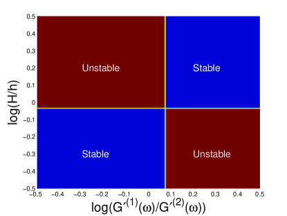
(b) $n>1$

Figure 2: Stability Diagram of the two layer configuration. The vertical neutral stability line is set by $G^{\prime(1)}(\omega)=nG^{\prime(2)}(\omega)$ while the horizontal line $h=\sqrt{n}H$. For example, we have taken: a) $n=5/6$ and b) $n=6/5$.

An important difference between our calculation and the case of Newtonian layers is the fact that here the up-down symmetry of the configuration is lost: $\sigma_{\text{el}}$ changes sign upon reversing the position of the fluid layers and their thicknesses. The sign of $\sigma_{\text{el}}(H,h,G^{*(2)}(\omega),G^{*(1)}(\omega))$ is opposite to the sign of $\sigma_{\text{el}}(h,H,G^{*(1)}(\omega),G^{*(2)}(\omega))$. Therefore, stability depends on which layer is adjacent to the boundary being sheared.

The instability mechanism in the Newtonian case arises from the out of phase evolution of the vorticity in both fluids hinch84 ; king99 . Small periodic distortions of the interface induce a vorticity perturbation of the same sign across the interface, but its sign alternates at each trough and peak. With negligible inertia, the vorticities are advected by the shear to create out of phase components of vorticity because of the viscosity contrast. As a result, vorticities of opposite sign at adjacent troughs and peaks get close together, and induce a vertical motion of the interface. The interfacial instability due to elasticity contrast found here has a similar origin in the out of phase vorticity as in the viscous case. The requirement that a viscosity contrast must exist ($n\neq 1$) for instability to occur ensures that there should exist an imbalance of vorticity across the interface. The essential difference between the viscous and elastic cases is that the out of phase motion of vorticity is driven in our case by the elasticity response. As can be seen from the complex wavevector of the base state, Eq. (21), elasticity induces a phase shift relative to the driving shear flow. Similarly, the elastic contrast of two fluids generates out of phase components of perturbed vorticity, and drives the interfacial instability.

IV Discussion

We discuss in this section the possible implications of our findings on orientation selection of block copolymers under shear. Following a quench of a large aspect ratio configuration (the aspect ratio being the ratio between the lateral dimension of the system and the lamellar spacing), a spontaneous distribution of locally ordered lamellar domains with random orientation results that coarsens with time re:elder92 . Under the application of a shear, the wavelength of those domains with orientation that has a transverse component ($\mathbf{\hat{q}}\parallel\mathbf{v}$) changes, fact that greatly reduces their range of stability re:chen02 . Therefore, after some initial transient, it is expected that a majority of domains would be oriented either parallel or perpendicular to the shear. Within the order parameter description used here, the local free energy of domains along the two orientations is the same, even under shear (since $\mathbf{\hat{q}}\cdot\mathbf{v}=0$). Hence, they are in coexistence.

As noted above, however, viscosity or elasticity of A or B rich regions are typically different. In PS-PI the glass transition temperature of the two blocks is quite different, and hence their mechanical response within the copolymer is expected to be different. However, given the small size of the blocks (on the order of tens of nm) and the large average viscosity of polymer melts, flows at the lamellar scale are expected to be negligible under most conditions of interest re:tamate08 . Furthermore, their contribution in slightly distorted lamellar configurations is of second order in the distortion, and do not contribute appreciably to their relaxation or stability re:chen02 . Therefore viscoleastic contrast between blocks seems insufficient to drive short scale flows that could account for differences between parallel and perpendicular orientations under shear.

Whereas short scale flows are strongly damped, this is not so for flows that couple to long range distortions of a lamellar configuration yoo12 , or flows at the scale of the characteristic domain size in a polycrystalline configuration. The analysis undertaken here has aimed at establishing the relative dynamic stability of parallel and perpendicular domains when long wavelength hydrodynamic flows are allowed. We have found that there exists an interfacial instability of hydrodynamic origin in that limit due to viscoelastic contrast between the two phases even for zero Reynolds number.

Domain coarsening and orientation selection are intrinsically nonlinear problems whereas we have only addressed here the linear stability of a particular configuration. The two can be qualitatively related as follows: Assume that after some transient there will be a preponderance of parallel and perpendicular domains in a large aspect ratio sample under oscillatory shear. The instability described will set in whenever two such domains meet, and the conditions for instability are satisfied (viscoelastic contrast) and low enough wavelength (or equivalently, a large enough characteristic domain size). Once any boundary between two such domains becomes unstable, a secondary flow is established which is normal to the boundary (shown schematically in Fig. 3). Advection of order parameter by this secondary flow distorts the parallel domain ($\mathbf{v}\parallel\mathbf{q}$) but not the perpendicular ($\mathbf{v}\perp\mathbf{q}$). The region with locally distorted parallel lamellae will have a higher free energy than the adjacent region of perpendicular lamellae, and boundary motion will follow to reduce the free energy imbalance. As a consequence, we would expect systematic motion of the boundary towards the parallel region every time there is a boundary instability. Although we cannot predict the nonlinear evolution of the boundary, and hence the evolution of an ensemble of domains in a large aspect ratio sample, this instability can provide for a dynamical selection mechanism that favors the perpendicular orientation whenever there is viscoelastic contrast between the two orientations. This result is generally consistent with the experimental survey of Ref. wu05, .

Three main issues remain unresolved. First, the argument presented does not account for the preponderance of the parallel orientation when there is no contrast. Second, as shown in Fig. 2, there are regions of parameter space in which the parallel-perpendicular boundary is stable. Therefore, whether a distribution of domains in a large aspect ratio sample would ultimately coarsen or evolve into coexistence cannot be conclusively answered by our analysis. Third, although there is ample evidence of viscoelastic contrast between differently oriented lamellae, there is no experimental study that we are aware of that has directly probed the uniaxial hydrodynamic properties of a bulk lamellar phase.

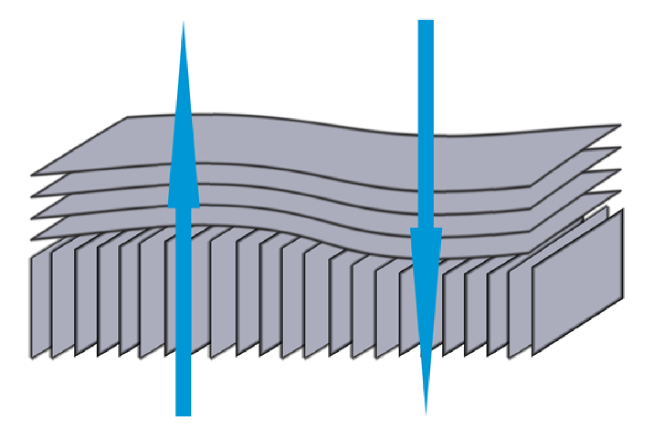
Figure 3: Orientation selection. The secondary flow induced by the unstable configuration is indicated by light blue arrows. This flow distorts the parallel lamellae without affecting the perpendicular lamellae.

Appendix A Expansion results for low Reynolds number and small elasticity

A.1 $\mathcal{O}(1)$ in $q_{x}$

At zeroth order in $q_{x}$ the momentum conservation equation Eq. (27) reduces to, with $\sigma_{0}=0$,

$$\rho\partial_{t}\partial_{z}^{2}\bar{\phi}_{0}^{(\alpha)}=\int_{-\infty}^{t}dt^{\prime}\;G^{(\alpha)}(t-t^{\prime})\partial_{z}^{4}\bar{\phi}_{0}^{(\alpha)}.$$ (52)

We have shown earlier that $\bar{\phi}_{0}^{(\alpha)}$ is time-periodic in $2\pi/\omega$, and given by Eq (41). For $e^{-i\omega t}$ mode, we have

$$-\frac{[cRe^{(\alpha)}]^{*}}{h^{2}}\partial_{z}^{2}\bar{\phi}_{0,-}^{(\alpha)}=\partial_{z}^{4}\bar{\phi}_{0,-}^{(\alpha)}.$$ (53)

For small $Re$, with Eq. (49), the above equation (52) becomes at zeroth order in $Re$

$$\partial_{z}^{4}\bar{\phi}_{0,-,0}^{(\alpha)}(z)=0,$$ (54)

and at first order in $Re$

$$\partial_{z}^{4}\bar{\phi}_{0,-,1}^{(\alpha)}=-\frac{i}{h^{2}}\frac{n^{(\alpha)}}{1+ig^{(\alpha)}}\partial_{z}^{2}\bar{\phi}_{0,-,0}^{(\alpha)}.$$ (55)

First, the general solution of Eq. (54) is

$$\bar{\phi}_{0,-,0}^{(\alpha)}(z)=A_{0}^{(\alpha)}+B_{0}^{(\alpha)}z+C_{0}^{(\alpha)}z^{2}+D_{0}^{(\alpha)}z^{3}.$$ (56)

The coefficients are determined by applying the boundary conditions Eqs. (29) - (34). At zeroth order in $Re$ the boundary conditions are

$$\bar{\phi}^{(2)}_{0,-,0}(z=H)=0,$$ (57)

$$\partial_{z}\bar{\phi}_{0,-,0}^{(2)}(z=H)=0,$$ (58)

$$\bar{\phi}_{0,-,0}^{(1)}(z=-h)=0,$$ (59)

$$\partial_{z}\bar{\phi}_{0,-,0}^{(1)}(z=-h)=0,$$ (60)

$$\bar{\phi}^{(2)}_{0,-,0}(z=0)=\bar{\phi}^{(1)}_{0,-,0}(z=0),$$ (61)

$$\partial_{z}u_{-,0}^{(2)}(z=0)\bar{z}_{s,0}+\partial_{z}\bar{\phi}^{(2)}_{0,-,0}(z=0)=\partial_{z}u_{-,0}^{(1)}(z=0)\bar{z}_{s,0}+\partial_{z}\bar{\phi}^{(1)}_{0,-,0}(z=0),$$ (62)

$$G^{*(2)}(-\omega)\partial_{z}^{2}\bar{\phi}_{0,-,0}^{(2)}(z=0)=G^{*(1)}(-\omega)\partial_{z}^{2}\bar{\phi}_{0,-,0}^{(1)}(z=0),$$ (63)

$$G^{*(2)}(-\omega)\partial_{z}^{3}\bar{\phi}_{0,-,0}^{(2)}(z=0)=G^{*(1)}(-\omega)\partial_{z}^{3}\bar{\phi}_{0,-,0}^{(1)}(z=0),$$ (64)

where the base flow is also expanded in $Re$

$$u_{-}^{(\alpha)}(z)=u_{-,0}^{(\alpha)}(z)+u_{-,1}^{(\alpha)}(z)Re+\mathcal{O}(Re^{2},(g^{(\alpha)})^{2}).$$ (65)

In terms of the coefficients of $\bar{\phi}_{0,-,0}^{(\alpha)}$ this set of boundary condition can be expressed as a 8$\times$8 matrix. We solve this linear system for the coefficients of $\bar{\phi}_{0,-,0}^{(\alpha)}(z)$ for small elasticity $g^{(\alpha)}\ll 1$, obtaining

$$A_{0}^{(1)} = A_{0}^{(2)}$$ (66)

$$= \frac{(H+h)h^{2}(n-1)nH^{2}\zeta_{0}U}{(h+nH)(n^{2}H^{4}+4nH^{3}h+6nH^{2}h^{2}+4nh^{3}H+h^{4})}$$

$$+i\frac{nU(H+h)\zeta_{0}H^{2}h^{2}(g^{(2)}-g^{(1)})}{(h+nH)^{2}(n^{2}H^{4}+4nH^{3}h+6nH^{2}h^{2}+4nh^{3}H+h^{4})^{2}}\times$$

$$\times(n^{4}H^{5}-2n^{3}H^{5}-5H^{4}n^{2}h-10n^{2}H^{3}h^{2}-10n^{2}H^{2}h^{3}$$

$$-5n^{2}Hh^{4}-2h^{5}n+h^{5})$$

$$B_{0}^{(1)} = \frac{(4nH^{3}+h^{3}+3nH^{2}h)(n-1)h\zeta_{0}U}{2(h+nH)(n^{2}H^{4}+4nH^{3}h+6nH^{2}h^{2}+4nh^{3}H+h^{4})}$$ (67)

$$+i\frac{nU\zeta_{0}h(g^{(2)}-g^{(1)})}{2(h+nH)^{2}(n^{2}H^{4}+4nH^{3}h+6nH^{2}h^{2}+4nh^{3}H+h^{4})^{2}}\times$$

$$\times(-5Hh^{7}-3H^{2}h^{6}+4n^{4}H^{8}-h^{8}-73n^{2}H^{5}h^{3}+2n^{3}H^{5}h^{3}$$

$$-20nH^{3}h^{5}-6n^{3}H^{7}h-10H^{4}nh^{4}-55H^{6}n^{2}h^{2}-45H^{4}n^{2}h^{4}$$

$$+4h^{6}n^{2}H^{2}-14h^{6}nH^{2}-9n^{2}H^{3}h^{5}+3n^{4}H^{7}h-20hH^{7}n^{2}-8n^{3}H^{8})$$

$$B_{0}^{(2)} = \frac{(H^{3}n+4h^{3}+3h^{2}H)(n-1)nH\zeta_{0}U}{2(h+nH)(n^{2}H^{4}+4nH^{3}h+6nH^{2}h^{2}+4nh^{3}H+h^{4})}$$ (68)

$$+i\frac{nUH\zeta_{0}(g^{(2)}-g^{(1)})}{2(h+nH)^{2}(n^{2}H^{4}+4nH^{3}h+6nH^{2}h^{2}+4nh^{3}H+h^{4})^{2}}\times$$

$$\times(n^{4}H^{8}+5n^{4}H^{7}h+3n^{4}H^{6}h^{2}+14n^{3}H^{6}h^{2}+20n^{3}H^{5}h^{3}$$

$$+10n^{3}H^{4}h^{4}-4n^{2}H^{6}h^{2}+9n^{2}h^{5}h^{3}+45n^{2}H^{4}h^{4}+73n^{2}H63h^{5}$$

$$+55n^{2}H^{2}h^{6}+20n^{2}Hh^{7}-2nH^{3}h^{5}+6nHh^{7}+8nh^{8}-3Hh^{7}-4h^{8})$$

$$C_{0}^{(1)} = \frac{1}{n}\Big{[}1+i(g^{(2)}-g^{(1)})\Big{]}C_{0}^{(2)}$$ (69)

$$= \frac{(H^{3}n+h^{3})(n-1)\zeta_{0}U}{(h+nH)(n^{2}H^{4}+4nH^{3}h+6nH^{2}h^{2}+4nh^{3}H+h^{4})}$$

$$+i\frac{nU\zeta_{0}(g^{(2)}-g^{(1)})}{(h+nH)^{2}(n^{2}H^{4}+4nH^{3}h+6nH^{2}h^{2}+4nh^{3}H+h^{4})^{2}}\times$$

$$\times(H^{8}n^{4}-2n^{3}H^{8}+2H^{5}n^{3}h^{3}-5hH^{7}n^{2}-10H^{6}n^{2}h^{2}$$

$$-13H^{5}n^{2}h^{3}+6n^{2}H^{3}h^{5}+4h^{6}n^{2}H^{2}-10H^{4}nh^{4}-14H^{3}nh^{5}$$

$$-8h^{6}n*H^{2}-3h^{5}H^{3}-6h^{6}H^{2}-5h^{7}H-h^{8})$$

$$D_{0}^{(1)} = \frac{1}{n}\Big{[}1+i(g^{(2)}-g^{(1)})\Big{]}D_{0}^{(2)}$$ (70)

$$= \frac{(h^{2}-nH^{2})(n-1)\zeta_{0}U}{2(h+nH)(n^{2}H^{4}+4nH^{3}h+6nH^{2}h^{2}+4nh^{3}H+h^{4})}$$

$$+i\frac{nU\zeta_{0}(g^{(2)}-g^{(1)})}{2(h+nH)^{2}(n^{2}H^{4}+4nH^{3}h+6nH^{2}h^{2}+4nh^{3}H+h^{4})^{2}}\times$$

$$\times(2n^{3}H^{7}-12h^{4}H^{3}n+4h^{5}n^{2}H^{2}+5n^{2}H^{6}h-7h^{5}H^{2}-5h^{6}H-h^{7}$$

$$-6h^{5}nH^{2}+15h^{3}H^{4}n^{2}+11h^{4}H^{3}n^{2}+2h^{2}n^{3}*H^{5}+7n^{2}H^{5}h^{2}$$

$$-10nH^{4}h^{3}-n^{4}H^{7}-4H^{3}h^{4})$$

At $\mathcal{O}(Re)$ the general solution to Eq. (55) is given by

$$\bar{\phi}_{0,-,1}^{(\alpha)}(z)=E_{0}^{(\alpha)}+F_{0}^{(\alpha)}z+J_{0}^{(\alpha)}z^{2}+L_{0}^{(\alpha)}z^{3}-\frac{i}{4h^{2}}\frac{n^{(\alpha)}}{1+ig^{(\alpha)}}\left(\frac{C_{0}^{(\alpha)}}{3}z^{4}+\frac{D_{0}^{(\alpha)}}{5}z^{5}\right)$$ (71)

where we have used Eq. (56) for the inhomogeneous term of Eq. (55). The boundary conditions at $\mathcal{O}(Re)$ are

$$\bar{\phi}^{(2)}_{0,-,1}(z=H)=0$$ (72)

$$\partial_{z}\bar{\phi}_{0,-,1}^{(2)}(z=H)=0$$ (73)

$$\bar{\phi}_{0,-,1}^{(1)}(z=-h)=0$$ (74)

$$\partial_{z}\bar{\phi}_{0,-,1}^{(1)}(z=-h)=0$$ (75)

$$\bar{\phi}^{(2)}_{0,-,1}(z=0)=\bar{\phi}^{(1)}_{0,-,1}(z=0)$$ (76)

$$\partial_{z}u_{-,1}^{(2)}(z=0)\bar{z}_{s,0}+\partial_{z}\bar{\phi}^{(2)}_{0,-,1}(z=0)=\partial_{z}u_{-,1}^{(1)}(z=0)\bar{z}_{s,0}+\partial_{z}\bar{\phi}^{(1)}_{0,-,1}(z=0)$$ (77)

$$G^{*(2)}(-\omega)\partial_{z}^{2}\bar{\phi}_{0,-,1}^{(2)}(z=0)=G^{*(1)}(-\omega)\partial_{z}^{2}\bar{\phi}_{0,-,1}^{(1)}(z=0)$$ (78)

$$G^{*(2)}(-\omega)\partial_{z}^{3}\bar{\phi}_{0,-,1}^{(2)}(z=0)=G^{*(1)}(-\omega)\partial_{z}^{3}\bar{\phi}_{0,-,1}^{(1)}(z=0)$$ (79)

which can also be written as a 8$\times$8 matrix for the coefficients of $\bar{\phi}_{0,-,1}^{(\alpha)}$. The solution is

$$E_{0}^{(1)} = E_{0}^{(2)}$$ (80)

$$= i\frac{(n-1)nU\zeta_{0}H^{2}}{60(h+nH)^{2}(n^{2}H^{4}+4nH^{3}h+6nH^{2}h^{2}+4nh^{3}H+h^{4})^{2}}\times$$

$$\times(8n^{4}H^{8}+9n^{4}H^{7}h+68n^{3}H^{7}h+140n^{3}H^{5}h^{3}+60H^{4}n^{3}h^{4}+152n^{3}H^{6}h^{2}$$

$$+120n^{2}H^{6}h^{2}+323n^{2}H^{5}h^{3}+370n^{2}H^{4}h^{4}+173n^{2}H^{3}h^{5}-130nH^{3}h^{5}$$

$$-82h^{7}nH-148nH^{2}h^{6}-60nH^{4}h^{4}-22h^{8}-21h^{7}H)$$

$$F_{0}^{(1)} = -i\frac{n(n-1)HU\zeta_{0}}{120h^{2}(h+nH)^{2}(n^{2}H^{4}+4nH^{3}h+6nH^{2}h^{2}+4nh^{3}H+h^{4})^{2}}\times$$ (81)

$$\times(10n^{5}H^{10}+80H^{7}n^{4}h^{3}+93H^{8}n^{4}h^{2}+78n^{4}H^{9}h+160H^{4}n^{3}h^{6}$$

$$+477H^{6}n^{3}h^{4}+128n^{3}H^{8}h^{2}+300H^{5}n^{3}h^{5}+305H^{7}n^{3}h^{3}+212H^{6}n^{2}h^{4}$$

$$+588H^{3}n^{2}h^{7}+1003H^{4}n^{2}h^{6}+817H^{5}n^{2}h^{5}-535h^{8}nH^{2}-497H^{3}nh^{7}$$

$$-328h^{9}nH-180nh^{6}H^{4}-88h^{10}-63h^{9}H)$$

$$F_{0}^{(2)} = i\frac{(n-1)U\zeta_{0}}{120h(h+nH)^{2}(n^{2}H^{4}+4nH^{3}h+6nH^{2}h^{2}+4nh^{3}H+h^{4})^{2}}\times$$ (82)

$$\times(32n^{5}H^{10}+27H^{9}n^{5}h+272n^{4}H^{9}h+515H^{8}n^{4}h^{2}+463H^{7}n^{4}h^{3}$$

$$+180H^{6}n^{4}h^{4}+480n^{3}H^{8}h^{2}+1068H^{7}n^{3}h^{3}+1123H^{6}n^{3}h^{4}+397H^{5}n^{3}h^{5}$$

$$-28H^{4}n^{3}h^{6}-320H^{6}n^{2}h^{4}-540H^{5}n^{2}h^{5}-543H^{4}n^{2}h^{6}-175H^{3}n^{2}h^{7}$$

$$+8h^{8}n^{2}H^{2}-160H^{3}nh^{7}-147h^{8}nH^{2}-72h^{9}nH-20h^{10})$$

$$J_{0}^{(1)} = \frac{1}{n}J_{0}^{(2)}$$ (83)

$$= i\frac{(n-1)U\zeta_{0}}{30h^{2}(h+nH)^{2}(n^{2}H^{4}+4nH^{3}h+6nH^{2}h^{2}+4nh^{3}H+h^{4})^{2}}\times$$

$$\times(4n^{5}H^{10}+20H^{7}n^{4}h^{3}+34n^{4}H^{9}h+27H^{8}n^{4}h^{2}-20H^{4}n^{3}h^{6}-16H^{6}n^{3}h^{4}$$

$$+37H^{7}n^{3}h^{3}-81H^{5}n^{3}h^{5}+60n^{3}H^{8}h^{2}+22H^{3}n^{2}h^{7}-80H^{6}n^{2}h^{4}$$

$$-96H^{5}n^{2}h^{5}-76H^{4}n^{2}h^{6}-48h^{8}nH^{2}-41h^{9}nH-55H^{3}nh^{7}-11h^{10})$$

$$L_{0}^{(1)} = -i\frac{(n-1)U\zeta_{0}}{120h^{2}(h+nH)^{2}(n^{2}H^{4}+4nH^{3}h+6nH^{2}h^{2}+4nh^{3}H+h^{4})^{2}}\times$$ (84)

$$\times(9n^{5}H^{9}+113n^{4}hH^{8}+106n^{4}h^{2}H^{7}+60n^{4}h^{3}H^{6}+324n^{3}h^{2}H^{7}$$

$$+522n^{3}h^{3}H^{6}+440n^{3}h^{4}H^{5}+64n^{3}h^{5}H^{4}+160n^{2}h^{3}H^{6}+176n^{2}h^{4}H^{5}$$

$$+160n^{2}h^{5}H^{4}-42n^{2}h^{6}H^{3}+36n^{2}h^{7}H^{2}+140nh^{6}H^{3}+134nh^{7}H^{2}$$

$$+127nh^{8}H+31h^{9})$$

$$L_{0}^{(2)} = i\frac{(n-1)nU\zeta_{0}}{120h^{2}(h+nH)^{2}(n^{2}H^{4}+4nH^{3}h+6nH^{2}h^{2}+4nh^{3}H+h^{4})^{2}}\times$$ (85)

$$\times(n^{5}H^{9}-23n^{4}hH^{8}+14n^{4}h^{2}H^{7}+20n^{4}h^{3}H^{6}-84n^{3}h^{2}H^{7}+78n^{3}h^{3}H^{6}$$

$$+340n^{3}h^{4}H^{5}+416n^{3}h^{5}H^{4}+160n^{3}h^{6}H^{3}+304n^{2}h^{4}H^{5}+620n^{2}h^{5}H^{4}$$

$$+642n^{2}h^{6}H^{3}+204n^{2}h^{7}H^{2}-60nh^{6}H^{3}-14nh^{7}H^{2}-37nh^{8}H-21h^{9})$$

A.2 $\mathcal{O}(q_{x})$

At $\mathcal{O}(q_{x})$, with $\sigma_{0}=\sigma_{1}=0$ the momentum conservation equation becomes

$$\rho\partial_{t}\partial_{z}^{2}\bar{\phi}_{1}^{(\alpha)}-\int_{-\infty}^{t}dt^{\prime}\;G^{(\alpha)}(t-t^{\prime})\partial_{z}^{4}\bar{\phi}_{1}^{(\alpha)}=i\rho\bar{\phi}_{0}^{(\alpha)}(\partial_{z}^{2}u_{b}^{(\alpha)})-i\rho u_{b}^{(\alpha)}\partial_{z}^{2}\bar{\phi}_{0}^{(\alpha)}$$ (86)

Since we are interested in the time-independent non-periodic part of $\bar{\phi}_{1}^{(\alpha)}$ in order to obtain the non-vanishing Floquet exponent $\sigma_{2}$, $\partial_{t}\bar{\phi}_{1,\text{NP}}=0$ and the momentum conservation equation reduces to

$$\partial_{z}^{4}\bar{\phi}_{1,\text{NP}}^{(\alpha)}=i\frac{\rho}{\eta^{(\alpha)}}\Big{[}u_{b}^{(\alpha)}\partial_{z}^{2}\bar{\phi}_{0}^{(\alpha)}-\bar{\phi}_{0}^{(\alpha)}\partial_{z}^{2}u_{b}^{(\alpha)}\Big{]}_{\text{NP}}$$ (87)

where the definition of the steady state viscosity is used

$$\eta^{(\alpha)}=\int_{0}^{\infty}dt\;G^{(\alpha)}(t),$$ (88)

and the non-periodic part of the RHS is given by

$$\Big{[}u_{b}^{(\alpha)}\partial_{z}^{2}\bar{\phi}_{0}^{(\alpha)}-\bar{\phi}_{0}^{(\alpha)}\partial_{z}^{2}u_{b}^{(\alpha)}\Big{]}_{\text{NP}}=\Big{[}u_{+}^{(\alpha)}\partial_{z}^{2}\bar{\phi}_{0,-}^{(\alpha)}+u_{-}^{(\alpha)}\partial_{z}^{2}\bar{\phi}_{0,+}^{(\alpha)}-\bar{\phi}_{0,-}^{(\alpha)}\partial_{z}^{2}u_{+}^{(\alpha)}-\bar{\phi}_{0,+}^{(\alpha)}\partial_{z}^{2}u_{-}^{(\alpha)}\Big{]}.$$ (89)

Again, in the same way to calculate the solution at $\mathcal{O}(1)$ in $q_{x}$ we take a solution expanding in small $Re$ as Eq. (50). Thus, at first two orders in $Re$ it is the case that

$$\partial_{z}^{4}\bar{\phi}_{1,\text{NP},0}^{(\alpha)}(z)=0,$$ (90)

$$\partial_{z}^{4}\bar{\phi}_{1,\text{NP},1}^{(\alpha)}=i\frac{n^{(\alpha)}}{\omega h^{2}}\Big{[}u_{+,0}^{(\alpha)}\partial_{z}^{2}\bar{\phi}_{0,-,0}^{(\alpha)}+u_{-,0}^{(\alpha)}\partial_{z}^{2}.\bar{\phi}_{0,+,0}^{(\alpha)}\Big{]}$$ (91)

The general solutions of Eqs. (90) and (91) are

$$\bar{\phi}_{1,\text{NP},0}^{(\alpha)}(z)=A_{1}^{(\alpha)}+B_{1}^{(\alpha)}z+C_{1}^{(\alpha)}z^{2}+D_{1}^{(\alpha)}z^{3}$$ (92)

$$\bar{\phi}_{1,\text{NP},1}^{(\alpha)}(z)=E_{1}^{(\alpha)}+F_{1}^{(\alpha)}z+J_{1}^{(\alpha)}z^{2}+L_{1}^{(\alpha)}z^{3}+\frac{\Lambda_{0}^{(\alpha)}}{24}z^{4}+\frac{\Lambda_{1}^{(\alpha)}}{120}z^{5}+\frac{\Lambda_{2}^{(\alpha)}}{360}z^{6}$$ (93)

where

$$\Lambda_{1}^{(\alpha)}=\frac{2in^{(\alpha)}}{\omega h^{2}}\Big{(}[u_{-,0}^{(\alpha)}(0)]^{*}C_{0}^{(\alpha)}+\text{c.c.}\Big{)}$$ (94)

$$\Lambda_{2}^{(\alpha)}=\frac{2in^{(\alpha)}}{\omega h^{2}}\Big{(}[\partial_{z}u_{-,0}^{(\alpha)}(0)]^{*}C_{0}^{(\alpha)}+3[u_{-,0}^{(\alpha)}(0)]^{*}D_{0}^{(\alpha)}+\text{c.c}\Big{)}$$ (95)

$$\Lambda_{3}^{(\alpha)}=\frac{6in^{(\alpha)}}{\omega h^{2}}\Big{(}[\partial_{z}u_{-,0}^{(\alpha)}(0)]^{*}D_{0}^{(\alpha)}+\text{c.c.}\Big{)}.$$ (96)

Similarly to the calculation at $\mathcal{O}(1)$ in $q_{x}$, the boundary conditions for $\bar{\phi}_{1,\text{NP},0}^{(\alpha)}(z)$ are

$$\bar{\phi}^{(2)}_{1,\text{NP},0}(z=H)=0,$$ (97)

$$\partial_{z}\bar{\phi}_{1,\text{NP},0}^{(2)}(z=H)=0,$$ (98)

$$\bar{\phi}_{1,\text{NP},0}^{(1)}(z=-h)=0,$$ (99)

$$\partial_{z}\bar{\phi}_{1,\text{NP},0}^{(1)}(z=-h)=0,$$ (100)

$$\bar{\phi}^{(2)}_{1,\text{NP},0}(z=0)=\bar{\phi}^{(1)}_{1,\text{NP},0}(z=0),$$ (101)

$$\partial_{z}\bar{\phi}^{(2)}_{1,\text{NP},0}(z=0)-\partial_{z}\bar{\phi}^{(1)}_{1,\text{NP},0}(z=0) = \frac{1}{\omega}\Big{[}\partial_{z}u_{+,0}^{(1)}-\partial_{z}u_{+,0}^{(2)}(z=0)\Big{]}_{z=0}\Big{[}z_{s,0}u_{-,0}^{(1)}+\bar{\phi}_{0,-,0}^{(1)}\Big{]}_{z=0}$$ (102)

$$-\text{c.c.},$$

$$\partial_{z}^{2}\bar{\phi}_{1,\text{NP},0}^{(2)}(z=0)=n\partial_{z}^{2}\bar{\phi}_{1,\text{NP},0}^{(1)}(z=0),$$ (103)

$$\partial_{z}^{3}\bar{\phi}_{1,\text{NP},0}^{(2)}(z=0)=n\partial_{z}^{3}\bar{\phi}_{1,\text{NP},0}^{(1)}(z=0),$$ (104)

and for $\bar{\phi}_{1,\text{NP},1}^{(\alpha)}(z)$

$$\bar{\phi}^{(2)}_{1,\text{NP},1}(z=H)=0,$$ (105)

$$\partial_{z}\bar{\phi}_{1,\text{NP},1}^{(2)}(z=H)=0,$$ (106)

$$\bar{\phi}_{1,\text{NP},1}^{(1)}(z=-h)=0,$$ (107)

$$\partial_{z}\bar{\phi}_{1,\text{NP},1}^{(1)}(z=-h)=0,$$ (108)

$$\bar{\phi}^{(2)}_{1,\text{NP},1}(z=0)=\bar{\phi}^{(1)}_{1,\text{NP},1}(z=0),$$ (109)

$$\partial_{z}\bar{\phi}^{(2)}_{1,\text{NP},1}(z=0)-\partial_{z}\bar{\phi}^{(1)}_{1,\text{NP},1}(z=0) = \frac{1}{\omega}\Big{[}\partial_{z}u_{+,0}^{(1)}-\partial_{z}u_{+,0}^{(2)}\Big{]}_{z=0}\Big{[}z_{s,0}u_{-,1}^{(1)}+\bar{\phi}_{0,-,1}^{(1)}\Big{]}_{z=0}$$ (110)

$$+\frac{1}{\omega}\Big{[}\partial_{z}u_{+,1}^{(1)}-\partial_{z}u_{+,1}^{(2)}\Big{]}_{z=0}\Big{[}z_{s,0}u_{-,0}^{(1)}+\bar{\phi}_{0,-,0}^{(1)}\Big{]}_{z=0}$$

$$-\text{c.c.},$$

$$\partial_{z}^{2}\bar{\phi}_{1,\text{NP},1}^{(2)}(z=0)=n\partial_{z}^{2}\bar{\phi}_{1,\text{NP},1}^{(1)}(z=0),$$ (111)

$$\partial_{z}^{3}\bar{\phi}_{1,\text{NP},1}^{(2)}(z=0)-n\partial_{z}^{3}\bar{\phi}_{1,\text{NP},1}^{(1)}(z=0) = \frac{in}{\omega h^{2}}\bar{\phi}_{0,-,0}^{(1)}(z=0)\Big{(}\partial_{z}u_{+,0}^{(1)}-\partial_{z}u_{+,0}^{(2)}\Big{)}_{z=0}$$ (112)

$$-\frac{in}{\omega h^{2}}u_{+,0}^{(1)}(z=0)\Big{(}\partial_{z}\bar{\phi}_{0,-,0}^{(1)}-\partial_{z}\bar{\phi}_{0,-,0}^{(2)}\Big{)}_{z=0}$$

$$-\text{c.c.},$$

can also be separately written as a $8\times 8$ matrix. The solutions are

$$A_{1}^{(1)} = A_{1}^{(2)}$$ (113)

$$= i\frac{h^{3}n^{2}U^{2}\zeta_{0}H^{2}(H+h)(g^{(2)}-g^{(1)})}{\omega(h+nH)^{2}(n^{2}H^{4}+4nH^{3}h+6nH^{2}h^{2}+4nh^{3}H+h^{4})^{3}}\times$$

$$\times(12nH^{3}h^{5}+14n^{2}h^{6}H^{2}+8h^{7}nH+16nH^{2}h^{6}+2n^{4}H^{6}h^{2}+18n^{2}H^{6}h^{2}-2h^{6}H^{2}$$

$$+h^{8}-2H^{3}h^{5}+n^{4}H^{8}+2n^{4}H^{7}h+4n^{3}H^{7}h+2n^{2}H^{7}h+46n^{2}H^{3}h^{5}+48n^{2}H^{5}h^{3}$$

$$+8n^{3}H^{5}h^{3}+8n^{3}H^{6}h^{2}+70n^{2}H^{4}h^{4})$$

$$B_{1}^{(1)} = -\frac{(4H^{3}n+h^{3}+3nH^{2}h)h}{n(H^{3}n+4h^{3}+3h^{2}H)H}B_{1}^{(2)}$$ (114)

$$= i\frac{nU^{2}\zeta_{0}h^{2}(4H^{3}n+h^{3}+3nH^{2}h)(g^{(2)}-g^{(1)})}{2\omega(h+nH)^{2}(n^{2}H^{4}+4nH^{3}h+6nH^{2}h^{2}+4nh^{3}H+h^{4})^{3}}\times$$

$$\times(8H^{5}n^{3}h^{3}+H^{8}n^{4}+70H^{4}n^{2}h^{4}+2n^{4}H^{6}h^{2}+12H^{3}nh^{5}+48H^{5}n^{2}h^{3}$$

$$+18H^{6}n^{2}h^{2}+2hH^{7}n^{2}+8H^{6}n^{3}h^{2}+46n^{2}H^{3}h^{5}+4H^{7}n^{3}h-2h^{5}H^{3}$$

$$+h^{8}+2n^{4}H^{7}h+16h^{6}nH^{2}-2h^{6}H^{2}+14h^{6}n^{2}H^{2}+8h^{7}nH)$$

$$C_{1}^{(1)} = \frac{1}{n}C_{1}^{(2)}$$ (115)

$$= i\frac{nU^{2}\zeta_{0}h(H^{3}n+h^{3})(g^{(2)}-g^{(1)})}{\omega(h+nH)^{2}(n^{2}H^{4}+4nH^{3}h+6nH^{2}h^{2}+4nh^{3}H+h^{4})^{3}}\times$$

$$\times(8H^{5}n^{3}h^{3}+H^{8}n^{4}+70H^{4}n^{2}h^{4}+2n^{4}H^{6}h^{2}+12H^{3}nh^{5}+48H^{5}n^{2}h^{3}$$

$$+18H^{6}n^{2}h^{2}+2hH^{7}n^{2}+8H^{6}n^{3}h^{2}+46n^{2}H^{3}h^{5}+4H^{7}n^{3}h-2h^{5}H^{3}$$

$$+h^{8}+2n^{4}H^{7}h+16h^{6}nH^{2}-2h^{6}H^{2}+14h^{6}n^{2}H^{2}+8h^{7}nH)$$

$$D_{1}^{(1)} = \frac{1}{n}D_{1}^{(2)}$$ (116)

$$= i\frac{nU^{2}\zeta_{0}h(h^{2}-nH^{2})(g^{(2)}-g^{(1)})}{2\omega(h+nH)^{2}(n^{2}H^{4}+4nH^{3}h+6nH^{2}h^{2}+4nh^{3}H+h^{4})^{3}}\times$$

$$\times(8H^{5}n^{3}h^{3}+H^{8}n^{4}+70H^{4}n^{2}h^{4}+2n^{4}H^{6}h^{2}+12H^{3}nh^{5}$$

$$+48H^{5}n^{2}h^{3}+18H^{6}n^{2}h^{2}+2hH^{7}n^{2}+8H^{6}n^{3}h^{2}+46n^{2}H^{3}h^{5}$$

$$+4H^{7}n^{3}h-2h^{5}H^{3}+h^{8}+2n^{4}H^{7}h+16h^{6}nH^{2}-2h^{6}H^{2}$$

$$+14h^{6}n^{2}H^{2}+8h^{7}nH)$$

$$E_{1}^{(1)} = E_{1}^{(2)}$$ (117)

$$= i\frac{n(n-1)\zeta_{0}U^{2}H^{2}}{120\omega(h+nH)^{2}(n^{2}H^{4}+4nH^{3}h+6nH^{2}h^{2}+4nh^{3}H+h^{4})^{3}}\times$$

$$\times(-224h^{8}n^{3}H^{4}+766h^{10}nH^{2}+304nh^{8}H^{4}+3884h^{7}n^{2}H^{5}+43h^{12}+2268h^{9}n^{2}H^{3}$$

$$632h^{10}n^{2}H^{2}-32H^{5}h^{7}n^{4}-16H^{8}h^{4}n^{5}+760h^{9}H^{3}n-12h^{3}H^{9}n^{5}+9h^{4}H^{8}n^{4}$$

$$-64h^{5}n^{4}H^{7}+332h^{11}nH-40h^{6}n^{4}H^{6}+176h^{5}H^{7}n^{3}+2040h^{6}H^{6}n^{2}-68h^{6}n^{3}H^{6}$$

$$+4027h^{8}n^{2}H^{4}-288h^{7}n^{3}H^{5}+4n^{6}hH^{11}+22n^{5}h^{2}H^{10}+94n^{4}h^{3}H^{9}+160n^{3}h^{4}H^{8}$$

$$n^{6}H^{12}+38h^{11}H+8n^{5}hH^{11}+24n^{4}h^{2}H^{10}+512n^{2}h^{5}H^{7})$$

$$F_{1}^{(1)} = i\frac{(n-1)\zeta_{0}U^{2}}{120h\omega(h+nH)^{2}(n^{2}H^{4}+4nH^{3}h+6nH^{2}h^{2}+4nh^{3}H+h^{4})^{3}}\times$$ (118)

$$\times(20h^{6}H^{8}n^{5}+452H^{6}h^{8}n^{4}+29H^{12}h^{2}n^{6}+384H^{10}h^{4}n^{4}$$

$$+2372H^{5}h^{9}n^{2}+6n^{7}hH^{13}+242H^{3}h^{11}n+307h^{12}nH^{2}+5046H^{5}h^{9}n^{3}$$

$$+1488h^{11}n^{2}H^{3}+1050H^{8}h^{6}n^{4}+103H^{10}h^{4}n^{5}+1340h^{10}H^{4}n^{3}+788H^{7}h^{7}n^{4}$$

$$+928H^{6}h^{8}n^{2}+58H^{9}h^{5}n^{5}+48n^{5}h^{2}H^{12}+166H^{11}h^{3}n^{5}-20n^{6}h^{3}H^{11}$$

$$+16n^{6}hH^{13}+154h^{13}nH+8820H^{6}h^{8}n^{3}+292h^{12}n^{2}H^{2}+240h^{9}H^{5}n^{4}$$

$$+2n^{7}H^{14}+2789H^{4}h^{10}n^{2}-24h^{4}H^{10}n^{6}+1120H^{9}h^{5}n^{3}-48h^{7}H^{7}n^{5}$$

$$+20h^{14}+828H^{9}h^{5}n^{4}+4432H^{8}h^{6}n^{3}+8536H^{7}h^{7}n^{3})$$

$$F_{1}^{(2)} = i\frac{n(n-1)\zeta_{0}U^{2}H}{120h\omega(h+nH)^{2}(n^{2}H^{4}+4nH^{3}h+6nH^{2}h^{2}+4nh^{3}H+h^{4})^{3}}\times$$ (119)

$$\times(-76n^{5}h^{4}H^{9}-848n^{4}h^{6}H^{7}-608n^{4}h^{7}H^{6}+2n^{6}h^{2}H^{11}-160n^{4}h^{8}H^{5}$$

$$-664nh^{12}H+10n^{6}hH^{12}-1337nh^{10}H^{3}-1020n^{3}h^{8}H^{5}-2400n^{3}h^{7}H^{6}$$

$$-3556n^{2}h^{7}H^{6}-2782n^{3}h^{6}H^{7}+12n^{5}hH^{12}-1264n^{2}h^{11}H^{2}+16n^{3}h^{9}H^{4}$$

$$-7100n^{2}h^{8}H^{5}-429n^{4}h^{4}H^{9}-768n^{2}h^{6}H^{7}-352n^{3}h^{4}H^{9}-7742n^{2}h^{9}H^{4}$$

$$-822n^{4}h^{5}H^{8}-1540n^{3}h^{5}H^{8}+23n^{5}h^{2}H^{11}-1406nh^{11}H^{2}-456nh^{9}H^{4}$$

$$-4434n^{2}h^{10}H^{3}-60n^{4}h^{3}H^{10}-86h^{13}+32n^{4}h^{2}H^{11}-34n^{5}h^{3}H^{10}$$

$$-32n^{5}h^{5}H^{8}+2n^{6}H^{13}-57h^{12}H)$$

$$J_{1}^{(1)} = \frac{1}{n}J_{1}^{(2)}$$ (120)

$$= i\frac{(n-1)\zeta_{0}U^{2}}{120\omega h^{2}(h+nH)^{2}(n^{2}H^{4}+4nH^{3}h+6nH^{2}h^{2}+4nh^{3}H+h^{4})^{3}}\times$$

$$\times(-8H^{12}h^{2}n^{6}+n^{7}H^{14}+6008H^{7}h^{7}n^{3}-4n^{6}h^{3}H^{11}+2464H^{7}h^{7}n^{4}$$

$$+1576H^{6}h^{8}n^{4}+2704H^{5}h^{9}n^{2}+480h^{9}H^{5}n^{4}+6093H^{6}h^{8}n^{3}+400H^{3}h^{11}n$$

$$+3574H^{4}h^{10}n^{2}+24n^{5}h^{2}H^{12}+1224H^{9}h^{5}n^{4}+832h^{10}H^{4}n^{3}+3080H^{8}h^{6}n^{3}$$

$$+8n^{6}hH^{13}+524h^{12}nH^{2}+2148h^{11}n^{2}H^{3}+332h^{13}nH+336H^{10}h^{4}n^{4}$$

$$+56H^{11}h^{3}n^{5}+1040H^{6}h^{8}n^{2}+800H^{9}h^{5}n^{3}+632h^{12}n^{2}H^{2}+308H^{9}h^{5}n^{5}$$

$$+3552H^{5}h^{9}n^{3}+160h^{6}H^{8}n^{5}+43h^{14}+2391H^{8}h^{6}n^{4}+182H^{10}h^{4}n^{5})$$

$$L_{1}^{(1)} = -i\frac{(n-1)\zeta_{0}U^{2}}{120\omega h^{2}(h+nH)^{2}(n^{2}H^{4}+4nH^{3}h+6nH^{2}h^{2}+4nh^{3}H+h^{4})^{3}}\times$$ (121)

$$\times(2n^{7}H^{13}-252nh^{10}H^{3}-29h^{13}-16n^{5}h^{6}H^{7}-1046n^{3}h^{8}H^{5}$$

$$-334nh^{11}H^{2}-90n^{5}h^{3}H^{10}-684n^{4}h^{4}H^{9}-436n^{2}h^{11}H^{2}-4n^{6}h^{2}H^{11}$$

$$-1104n^{3}h^{5}H^{8}-1896n^{3}h^{7}H^{6}+15n^{6}hH^{12}-186n^{5}h^{4}H^{9}-900n^{4}h^{7}H^{6}$$

$$-2060n^{3}h^{6}H^{7}-1296n^{2}h^{1}0H^{3}-100n^{5}h^{5}H^{8}-1492n^{2}h^{8}H^{5}-226nh^{12}H$$

$$-156n^{3}h^{9}H^{4}-176n^{4}h^{3}H^{10}-2059n^{2}h^{9}H^{4}-576n^{2}h^{7}H^{6}+8n^{5}h^{2}H^{11}$$

$$-320n^{3}h^{4}H^{9}-8n^{6}h^{3}H^{10}-1367n^{4}h^{5}H^{8}-240n^{4}h^{8}H^{5}-1404n^{4}h^{6}H^{7})$$

$$L_{1}^{(2)} = -i\frac{n(n-1)\zeta_{0}U^{2}}{120\omega h^{2}(h+nH)^{2}(n^{2}H^{4}+4nH^{3}h+6nH^{2}h^{2}+4nh^{3}H+h^{4})^{3}}\times$$ (122)

$$\times(320n^{4}h^{9}H^{4}+2n^{7}H^{13}+800n^{3}h^{10}H^{3}-152nh^{10}H^{3}-19h^{13}$$

$$+144n^{5}h^{6}H^{7}+4554n^{3}h^{8}H^{5}-174nh^{11}H^{2}+230n^{5}h^{3}H^{10}+676n^{4}h^{4}H^{9}$$

$$+64n^{2}h^{11}H^{2}+16n^{6}h^{2}H^{11}+496n^{3}h^{5}H^{8}+4184n^{3}h^{7}H^{6}+25n^{6}hH^{12}$$

$$+334n^{5}h^{4}H^{9}+1940n^{4}h^{7}H^{6}+2060n^{3}h^{6}H^{7}+4n^{2}h^{10}H^{3}+300n^{5}h^{5}H^{8}$$

$$-452n^{2}h^{8}H^{5}-106nh^{12}H+2804n^{3}h^{9}H^{4}+144n^{4}h^{3}H^{10}-389n^{2}h^{9}H^{4}$$

$$-256n^{2}h^{7}H^{6}+108n^{5}h^{2}H^{11}+12n^{6}h^{3}H^{10}+1583n^{4}h^{5}H^{8}+1040n^{4}h^{8}H^{5}$$

$$+2236n^{4}h^{6}H^{7})$$

We now obtain the Floquet exponent Eq. (51) using Eqs. (66), (80), (113) and (117), resulting in

$$\sigma_{\text{el}} = \frac{U^{2}h^{3}H^{2}n(H+h)(n-1)(nH^{2}-h^{2})(nH^{2}+h^{2})(g^{(2)}-g^{(1)})}{\omega(h+nH)^{2}}\times$$ (123)

$$\times\frac{n^{2}H^{4}+2hn^{2}H^{3}+2H^{2}n^{2}h^{2}+2nH^{3}h+4nH^{2}h^{2}+4h^{3}nH+h^{4}}{(h^{4}+6nH^{2}h^{2}+n^{2}H^{4}+4h^{3}nH+4nH^{3}h)^{3}}$$

and

$$\sigma_{\text{vis}} = \frac{U^{2}H^{2}n(n-1)(4hn^{2}H^{3}+n^{2}H^{4}+h^{4}+4h^{3}H+6nH^{2}h^{2})}{120\omega(h+nH)^{2}(h^{4}+6nH^{2}h^{2}+n^{2}H^{4}+4h^{3}nH+4nH^{3}h)^{3}}\times$$ (124)

$$\times(n^{4}H^{8}+4n^{3}H^{7}h-2n^{3}H^{6}h^{2}-4h^{3}n^{3}H^{5}+8n^{2}H^{6}h^{2}+8n^{2}H^{5}h^{3}$$

$$\hskip 14.22636pt-8h^{5}n^{2}H^{3}-8h^{6}n^{2}H^{2}+4h^{5}nH^{3}+2h^{6}nH^{2}-4h^{7}nH-h^{8})$$

Appendix B Expansion for general Reynolds number

Now we present a general framework to obtain a solution of the equations of motion for an arbitrary Reynolds number, but still in the limit of small $q_{x}$.

B.1 $\mathcal{O}(1)$

For arbitrary Reynolds number we can find a general solution to Eq. (52) by taking Eq. (41) for $\bar{\phi}_{0}^{(\alpha)}$. For $e^{-i\omega t}$ mode the general solution to Eq. (52) is

$$\bar{\phi}_{0,-}^{(\alpha)}(z)=\hat{A}_{0}^{(\alpha)}+\hat{B}_{0}^{(\alpha)}z+\hat{C}_{0}^{(\alpha)}e^{k^{(\alpha)}z}+\hat{D}_{0}^{(\alpha)}e^{-k^{(\alpha)}z}$$ (125)

where $k^{(\alpha)}$ is given by Eq. (21). Again, the coefficients of $\bar{\phi}_{0,-}^{(\alpha)}(z)$ are determined by applying the boundary conditions, Eqs. (29) - (34) which are

$$\hat{A}_{0}^{(2)}+\hat{B}_{0}^{(2)}H+\hat{C}_{0}^{(2)}e^{k^{(2)}H}+\hat{D}_{0}^{(2)}e^{-k^{(2)}H}=0$$ (126)

$$\hat{B}_{0}^{(2)}+k^{(2)}\hat{C}_{0}^{(2)}e^{k^{(2)}H}-k^{(2)}\hat{D}_{0}^{(2)}e^{-k^{(2)}H}=0$$ (127)

$$\hat{A}_{0}^{(1)}-\hat{B}_{0}^{(1)}h+\hat{C}_{0}^{(1)}e^{-k^{(1)}h}+\hat{D}_{0}^{(1)}e^{k^{(1)}h}=0$$ (128)

$$\hat{B}_{0}^{(1)}+k^{(1)}\hat{C}_{0}^{(1)}e^{-k^{(1)}h}-k^{(1)}\hat{D}_{0}^{(1)}e^{k^{(1)}h}=0$$ (129)

$$\hat{A}_{0}^{(2)}+\hat{C}_{0}^{(2)}+\hat{D}_{0}^{(2)}=\hat{A}_{0}^{(1)}+\hat{C}_{0}^{(1)}+\hat{D}_{0}^{(1)}$$ (130)

$$\frac{1}{2}\partial_{z}u_{0}^{(2)}(z=0)\zeta_{0}+\hat{B}_{0}^{(2)}+k^{(2)}\hat{C}_{0}^{(2)}-k^{(2)}\hat{D}_{0}^{(2)}=\frac{1}{2}\partial_{z}u_{0}^{(1)}(z=0)\zeta_{0}+\hat{B}_{0}^{(1)}+k^{(1)}\hat{C}_{0}^{(1)}-k^{(1)}\hat{D}_{0}^{(1)}$$ (131)

$$\hat{C}_{0}^{(2)}+\hat{D}_{0}^{(2)}=\hat{C}_{0}^{(1)}+\hat{D}_{0}^{(1)}$$ (132)

$$\hat{B}_{0}^{(2)}=\hat{B}_{0}^{(1)}$$ (133)

Therefore we obtain $\bar{\phi}_{0}^{(\alpha)}$ by solving this 8$\times$8 linear system.

B.2 $\mathcal{O}(q_{x})$

At $\mathcal{O}(q_{x})$, we have to solve Eq. (87) for $\bar{\phi}_{1,\text{NP}}^{(\alpha)}$. If Eq. (125) is used in the RHS of Eq. (87), we get

$$\eta^{(\alpha)}\partial_{z}^{4}\bar{\phi}_{1,\text{NP}}^{(\alpha)} = i\rho\Big{[}(k^{(\alpha)})^{2}-(k^{(\alpha)*})^{2}\Big{]}u_{+}^{(\alpha)}\Big{[}\hat{C}_{0}^{(\alpha)}e^{k^{(\alpha)}z}+\hat{D}_{0}^{(\alpha)}e^{-k^{(\alpha)}z}\Big{]}$$ (134)

$$-i\rho(k^{(\alpha)*})^{2}u_{+}^{(\alpha)}(\hat{A}_{0}^{(\alpha)}+\hat{B}_{0}^{(\alpha)}z)-\text{c.c.}$$

The solution to the above differential equation has a homogeneous solution $\bar{\phi}_{1,\text{NP},h}^{(\alpha)}$ and a particular solution $\bar{\phi}_{1,\text{NP},p}^{(\alpha)}$. First, the particular solution can be found by using the fact that

$$\partial_{z}^{4}f(z)=(A+Bz)e^{\pm kz},$$ (135)

so that

$$f_{p}(z)=\Bigg{(}\frac{A}{k^{4}}\mp 4\frac{B}{k^{5}}+\frac{B}{k^{4}}z\Bigg{)}e^{\pm kz},$$ (136)

and, similarly,

$$\partial_{z}^{4}g(z)=Ce^{\pm kz},$$ (137)

$$g_{p}(z)=\frac{C}{k^{4}}e^{\pm kz}.$$ (138)

The resulting particular solution for fluid 1 is

$$\bar{\phi}^{(1)}_{1,\text{NP},p} = -\frac{i}{4}\frac{\rho}{\eta^{(1)}}(k^{(1)*})^{2}\frac{U}{K^{*}}\Bigg{[}\frac{\hat{A}_{0}^{(1)}}{(k^{(1)*})^{4}}-4\frac{\hat{B}_{0}^{(1)}}{(k^{(1)*})^{5}}+\frac{\hat{B}_{0}^{(1)}}{(k^{(1)*})^{4}}z\Bigg{]}e^{k^{(1)*}(z+h)}$$ (139)

$$+\frac{i}{4}\frac{\rho}{\eta^{(1)}}(k^{(1)*})^{2}\frac{U}{K^{*}}\Bigg{[}\frac{\hat{A}_{0}^{(1)}}{(k^{(1)*})^{4}}+4\frac{\hat{B}_{0}^{(1)}}{(k^{(1)*})^{5}}+\frac{\hat{B}_{0}^{(1)}}{(k^{(1)*})^{4}}z\Bigg{]}e^{-k^{(1)*}(z+h)}$$

$$+\frac{i}{4}\frac{\rho}{\eta^{(1)}}\Big{[}(k^{(1)})^{2}-(k^{(1)*})^{2}\Big{]}\frac{U}{K^{*}}e^{k^{(1)*}h}$$

$$\hskip 28.45274pt\times\Bigg{[}\frac{\hat{C}_{0}^{(1)}}{(k^{(1)*}+k^{(1)})^{4}}e^{(k^{(1)*}+k^{(1)})z}+\frac{\hat{D}_{0}^{(1)}}{(k^{(1)*}-k^{(1)})^{4}}e^{(k^{(1)*}-k^{(1)})z}\Bigg{]}$$

$$-\frac{i}{4}\frac{\rho}{\eta^{(1)}}\Big{[}(k^{(1)})^{2}-(k^{(1)*})^{2}\Big{]}\frac{U}{K^{*}}e^{-k^{(1)*}h}$$

$$\hskip 28.45274pt\times\Bigg{[}\frac{\hat{C}_{0}^{(1)}}{(k^{(1)*}-k^{(1)})^{4}}e^{-(k^{(1)*}-k^{(1)})z}+\frac{\hat{D}_{0}^{(1)}}{(k^{(1)*}+k^{(1)})^{4}}e^{-(k^{(1)*}+k^{(1)})z}\Bigg{]}$$

$$-\text{c.c.}$$

and for fluid 2

$$\bar{\phi}^{(2)}_{1,\text{NP},p} = -\frac{i}{4}\frac{\rho}{\eta^{(2)}}(k^{(2)*})^{2}\frac{U}{K^{*}}\sinh(k^{(1)*}h)\Bigg{[}\frac{\hat{A}_{0}^{(2)}}{(k^{(2)*})^{4}}-4\frac{\hat{B}_{0}^{(2)}}{(k^{(2)*})^{5}}+\frac{\hat{B}_{0}^{(2)}}{(k^{(2)*})^{4}}z\Bigg{]}e^{k^{(2)*}z}$$ (140)

$$-\frac{i}{4}\frac{\rho}{\eta^{(2)}}(k^{(2)*})^{2}\frac{U}{K^{*}}\sinh(k^{(1)*}h)\Bigg{[}\frac{\hat{A}_{0}^{(2)}}{(k^{(2)*})^{4}}+4\frac{\hat{B}_{0}^{(2)}}{(k^{(2)*})^{5}}+\frac{\hat{B}_{0}^{(2)}}{(k^{(2)*})^{4}}z\Bigg{]}e^{-k^{(2)*}z}$$

$$-\frac{i}{4}\frac{\rho}{\eta^{(2)}}(k^{(2)*})^{2}\frac{U}{K^{*}}\frac{G^{*(1)}(\omega)k^{(1)*}}{G^{*(2)}(\omega)k^{(2)*}}\cosh(k^{(1)*}h)\Bigg{[}\frac{\hat{A}_{0}^{(2)}}{(k^{(2)*})^{4}}-4\frac{\hat{B}_{0}^{(2)}}{(k^{(2)*})^{5}}+\frac{\hat{B}_{0}^{(2)}}{(k^{(2)*})^{4}}z\Bigg{]}e^{k^{(2)*}z}$$

$$+\frac{i}{4}\frac{\rho}{\eta^{(2)}}(k^{(2)*})^{2}\frac{U}{K^{*}}\frac{G^{*(1)}(\omega)k^{(1)*}}{G^{*(2)}(\omega)k^{(2)*}}\cosh(k^{(1)*}h)\Bigg{[}\frac{\hat{A}_{0}^{(2)}}{(k^{(2)*})^{4}}+4\frac{\hat{B}_{0}^{(2)}}{(k^{(2)*})^{5}}+\frac{\hat{B}_{0}^{(2)}}{(k^{(2)*})^{4}}z\Bigg{]}e^{-k^{(2)*}z}$$

$$+\frac{i}{4}\frac{\rho}{\eta^{(2)}}\Big{[}(k^{(2)})^{2}-(k^{(2)*})^{2}\Big{]}\frac{U}{K^{*}}\sinh(k^{(1)*}h)$$

$$\hskip 14.22636pt\times\Bigg{[}\hat{C}_{0}^{(2)}\Bigg{(}\frac{e^{(k^{(2)*}+k^{(2)})z}}{(k^{(2)*}+k^{(2)})^{4}}+\frac{e^{(k^{(2)*}-k^{(2)})z}}{(k^{(2)*}-k^{(2)})^{4}}\Bigg{)}+\hat{D}_{0}^{(1)}\Bigg{(}\frac{e^{-(k^{(2)*}+k^{(2)})z}}{(k^{(2)*}-k^{(2)})^{4}}+\frac{e^{-(k^{(2)*}-k^{(2)})z}}{(k^{(2)*}+k^{(2)})^{4}}\Bigg{)}\Bigg{]}$$

$$+\frac{i}{4}\frac{\rho}{\eta^{(2)}}\Big{[}(k^{(2)})^{2}-(k^{(2)*})^{2}\Big{]}\frac{U}{K^{*}}\frac{G^{*(1)}(\omega)k^{(1)*}}{G^{*(2)}(\omega)k^{(2)*}}\cosh(k^{(1)*}h)$$

$$\hskip 14.22636pt\times\Bigg{[}\hat{C}_{0}^{(2)}\Bigg{(}\frac{e^{(k^{(2)*}+k^{(2)})z}}{(k^{(2)*}+k^{(2)})^{4}}-\frac{e^{-(k^{(2)*}-k^{(2)})z}}{(k^{(2)*}-k^{(2)})^{4}}\Bigg{)}+\hat{D}_{0}^{(1)}\Bigg{(}\frac{e^{(k^{(2)*}+k^{(2)})z}}{(k^{(2)*}-k^{(2)})^{4}}-\frac{e^{-(k^{(2)*}-k^{(2)})z}}{(k^{(2)*}+k^{(2)})^{4}}\Bigg{)}\Bigg{]}$$

$$-\text{c.c.}$$

Note that $\bar{\phi}_{1,\text{NP},p}^{(\alpha)}(z)$ is purely imaginary. On the other hand, the homogeneous solution is

$$\bar{\phi}^{(\alpha)}_{1,\text{NP},h}=\hat{A}_{1}^{(\alpha)}+\hat{B}_{1}^{(\alpha)}z+\hat{C}_{1}^{(\alpha)}z^{2}+\hat{D}_{1}^{(\alpha)}z^{3}$$ (141)

The eight coefficients of $\bar{\phi}^{(\alpha)}_{1,\text{NP},h}$ are determined by imposing the eight boundary conditions.

$$\bar{\phi}_{1,\text{NP},h}^{(2)}(z=H)+\bar{\phi}_{1,\text{NP},p}^{(2)}(z=H)=0$$ (142)

$$\partial_{z}\bar{\phi}_{1,\text{NP},h}^{(2)}(z=H)+\partial_{z}\bar{\phi}_{1,\text{NP},p}^{(2)}(z=H)=0$$ (143)

$$\bar{\phi}_{1,\text{NP},h}^{(1)}(z=-h)+\bar{\phi}_{1,\text{NP},p}^{(1)}(z=-h)=0$$ (144)

$$\partial_{z}\bar{\phi}_{1,\text{NP},h}^{(1)}(z=-h)+\partial_{z}\bar{\phi}_{1,\text{NP},p}^{(1)}(z=-h)=0$$ (145)

$$\bar{\phi}_{1,\text{NP},h}^{(2)}(z=0)+\bar{\phi}_{1,\text{NP},p}^{(2)}(z=0)=\bar{\phi}_{1,\text{NP},h}^{(1)}(z=0)+\bar{\phi}_{1,\text{NP},p}^{(1)}(z=0)$$ (146)

$$\begin{split}\Big{[}\partial_{z}u_{b}^{(2)}(z=0)&\bar{z}_{s,1}\Big{]}_{\text{NP}}+\partial_{z}\Big{[}\bar{\phi}_{1,\text{NP},h}^{(2)}+\bar{\phi}_{1,\text{NP},p}^{(2)}\Big{]}_{z=0}\\ &=\Big{[}\partial_{z}u_{b}^{(1)}(z=0)\bar{z}_{s,1}\Big{]}_{\text{NP}}+\partial_{z}\Big{[}\bar{\phi}_{1,\text{NP},h}^{(1)}+\bar{\phi}_{1,\text{NP},p}^{(1)}\Big{]}_{z=0}\end{split}$$ (147)

$$\eta^{(2)}\partial_{z}^{2}\Big{[}\bar{\phi}_{1,\text{NP},h}^{(2)}+\bar{\phi}_{1,\text{NP},p}^{(2)}\Big{]}_{z=0}=\eta^{(1)}\partial_{z}^{2}\Big{[}\bar{\phi}_{1,\text{NP},h}^{(1)}+\bar{\phi}_{1,\text{NP},p}^{(1)}\Big{]}_{z=0}$$ (148)

$$\begin{split}&i\rho\Big{[}u_{b}^{(2)}\partial_{z}\bar{\phi}_{0}^{(2)}-\bar{\phi}_{0}^{(2)}\partial_{z}u_{b}^{(2)}\Big{]}_{\text{NP},z=0}-\eta^{(2)}\partial_{z}^{3}\Big{[}\bar{\phi}_{1,\text{NP},h}^{(2)}+\bar{\phi}_{1,\text{NP},p}^{(2)}\Big{]}_{z=0}\\ &=i\rho\Big{[}u_{b}^{(1)}\partial_{z}\bar{\phi}_{0}^{(1)}-\bar{\phi}_{0}^{(1)}\partial_{z}u_{b}^{(1)}\Big{]}_{\text{NP},z=0}-\eta^{(1)}\partial_{z}^{3}\Big{[}\bar{\phi}_{1,\text{NP},h}^{(1)}+\bar{\phi}_{1,\text{NP},p}^{(1)}\Big{]}_{z=0}\end{split}$$ (149)

Again, the general solution can be found by solving this 8$\times$8 matrix for the coefficients of $\bar{\phi}_{1,\text{NP},h}^{(\alpha)}$

In principle, we can get $\sigma_{2}$ of Eq. (46) from the derived solutions $\bar{\phi}_{1,\text{NP},h}^{(\alpha)}$ and $\bar{\phi}_{1,\text{NP},p}^{(\alpha)}$

$$\sigma_{2}=-i\frac{q^{2}}{\zeta_{0}}\bigg{\{}\Big{[}u_{b}^{(1)}|_{z=0}\bar{z}_{s,1}\Big{]}_{\text{NP}}+\bar{\phi}_{1,\text{NP},h}^{(\alpha)}|_{z=0}+\bar{\phi}_{1,\text{NP},p}^{(\alpha)}|_{z=0}\bigg{\}}$$ (150)

where

$$\Big{[}u_{b}^{(\alpha)}|_{z=0}\bar{z}_{s,1}\Big{]}_{\text{NP}}=\frac{1}{\omega}\Big{\{}[u_{0,-}^{(1)}]^{*}\hat{A}_{0}^{(1)}-\text{c.c.}\Big{\}}_{z=0}$$ (151)

and

$$\bar{\phi}_{1,\text{NP},h}^{(\alpha)}|_{z=0}=\hat{A}_{1}^{(1)}$$ (152)

$$\bar{\phi}_{1,\text{NP},p}^{(\alpha)}|_{z=0} = -\frac{i}{4}\frac{\rho}{\eta^{(1)}}(k^{(1)*})^{2}\frac{U}{K^{*}}e^{k^{(1)*}h}\Bigg{[}\frac{\hat{A}_{0}^{(1)}}{(k^{(1)*})^{4}}-4\frac{\hat{B}_{0}^{(1)}}{(k^{(1)*})^{5}}\Bigg{]}$$ (153)

$$+\frac{i}{4}\frac{\rho}{\eta^{(1)}}(k^{(1)*})^{2}\frac{U}{K^{*}}e^{-k^{(1)*}h}\Bigg{[}\frac{\hat{A}_{0}^{(1)}}{(k^{(1)*})^{4}}+4\frac{\hat{B}_{0}^{(1)}}{(k^{(1)*})^{5}}\Bigg{]}$$

$$+\frac{i}{4}\frac{\rho}{\eta^{(1)}}\Big{[}(k^{(1)})^{2}-(k^{(1)*})^{2}\Big{]}\frac{U}{K^{*}}e^{k^{(1)*}h}\Bigg{[}\frac{\hat{C}_{0}^{(1)}}{(k^{(1)*}+k^{(1)})^{4}}+\frac{\hat{D}_{0}^{(1)}}{(k^{(1)*}-k^{(1)})^{4}}\Bigg{]}$$

$$-\frac{i}{4}\frac{\rho}{\eta^{(1)}}\Big{[}(k^{(1)})^{2}-(k^{(1)*})^{2}\Big{]}\frac{U}{K^{*}}e^{-k^{(1)*}h}\Bigg{[}\frac{\hat{C}_{0}^{(1)}}{(k^{(1)*}-k^{(1)})^{4}}+\frac{\hat{D}_{0}^{(1)}}{(k^{(1)*}+k^{(1)})^{4}}\Bigg{]}$$

$$-\text{c.c.}$$

In general, $\sigma_{2}$ is too a complicated function of fluid parameters to present explicitly, but we can readily evaluate it numerically. However, one should be careful in the numerical evaluation as we have observed numerical instabilities in certain limits. For example, in the limit of small Reynolds number $\Re[k^{(\alpha)}]$ becomes too small, and causes singular behavior, leaving the numerical result unreliable. In this regard, we decided to work directly on the limit of small Reynolds number as done in Appendix A

References

(1)
C. Park, J. Yoon, and E. Thomas, Polymer 44, 7779 (2003).
(2)
C. Black, Appl. Phys. Lett. 87, 163116 (2005).
(3)
D. Zschech et al., Nano Lett. 42, 1516 (2007).
(4)
C. Tang et al., Science 322, 429 (2008).
(5)
S. Pujari, M. Keaton, P. Chaikin, and R. Register, Soft Matter 8, 5358
(2012).
(6)
N. Xie, W. Li, F. Qiu, and A.-C. Shi, Soft Matter 9, 536 (2013).
(7)
K. Yamada, M. Nonomura, and T. Ohta, Macromolecules 37, 5762 (2004).
(8)
Z. Guo et al., Phys. Rev. Lett. 101, 028301 (2008).
(9)
S. Lee, M. Bluemle, and F. Bates, Science 330, 349 (2010).
(10)
C. Harrison et al., Science 290, 1558 (2000).
(11)
S. Kim et al., Nature 424, 411 (2003).
(12)
E. Kramer, Nature 437, 824 (2005).
(13)
J. K. Bosworth et al., J. Photopolymer Sci. and Tech. 20, 519
(2007).
(14)
D. Angelescu et al., Adv. Mater. 16, 1736 (2004).
(15)
D. Angelescu, J. Waller, R. Register, and P. Chaikin, Adv. Mater. 17,
1878 (2005).
(16)
Y. Zhang, U. Wiesner, and H. Spiess, Macromolecules 28, 778 (1995).
(17)
S. Patel, R. Larson, K. Winey, and H. Watanabe, Macromolecules 28, 4313
(1995).
(18)
Z.-R. Chen and J. A. Kornfield, Polymer 39, 4679 (1998).
(19)
L. Wu, T. Lodge, and F. Bates, J. Rheol. 49, 1231 (2005).
(20)
V. Olszowka, L. Tsarkova, and A. Boker, Soft Matter 5, 812 (2009).
(21)
G. Fredrickson and F. Bates, Annu. Rev. Mater. Sci. 26, 501 (1996).
(22)
K. Koppi et al., J. Phys. II France 2, 1941 (1992).
(23)
R. Larson et al., Rheologica Acta 32, 245 (1993).
(24)
V. Gupta, R. Krishnamoorti, J. Kornfield, and S. Smith, Macromolecules 28, 4464 (1995).
(25)
J. Rosedale and F. Bates, Macromolecules 23, 2329 (1990).
(26)
P. Martin, O. Parodi, and P. Pershan, Phys. Rev. A 6, 2401 (1972).
(27)
Z.-F. Huang and J. Viñals, J. Rheol. 51, 99 (2007).
(28)
P. Chen and J. Viñals, Macromolecules 35, 4183 (2002).
(29)
G. Fredrickson, J. Rheol. 38, 1045 (1994).
(30)
C.-S. Yih, J. Fluid Mech. 27, 337 (1967).
(31)
C.-S. Yih, J. Fluid Mech. 31, 737 (1968).
(32)
A. Hooper and W. Boyd, J. Fluid Mech. 128, 507 (1983).
(33)
E. Hinch, J. Fluid Mech. 144, 463 (1984).
(34)
M. King, D. Leighton, and M. McCready, Phys. Fluids 11, 833 (1999).
(35)
C.-H. Li, Phys. Fluids 12, 531 (1969).
(36)
N. Waters and A. Keeley, J. Non-Newtonian Fluid Mech. 24, 161 (1987).
(37)
Y. Renardy, J. Non-Newtonian Fluid Mech. 28, 99 (1988).
(38)
K. Chen, J. Non-Newtonian Fluid Mech. 40, 261 (1991).
(39)
J. Ferry, Viscoelastic properties of polymers (New York, Wiley, New York,
1970), (John D.) Includes bibliographies.
(40)
K. Elder, J. Viñals, and M. Grant, Phys. Rev. Lett. 68, 3024
(1992).
(41)
R. Tamate, K. Yamada, J. Viñals, and T. Ohta, J. Phys. Soc. Jpn. 78,
034802 (2008).
(42)
C.-D. Yoo and J. Viñals, Macromolecules 45, 4848 (2012).