Abstract. The unified gas kinetic scheme (UGKS) of K. Xu et al. [37], originally developed for multiscale gas dynamics problems, is applied in this paper to a linear kinetic model of radiative transfer theory. While such problems exhibit purely diffusive behavior in the optically thick (or small Knudsen) regime, we prove that UGKS is still asymptotic preserving (AP) in this regime, but for the free transport regime as well. Moreover, this scheme is modified to include a time implicit discretization of the limit diffusion equation, and to correctly capture the solution in case of boundary layers. Contrary to many AP schemes, this method is based on a standard finite volume approach, it does neither use any decomposition of the solution, nor staggered grids. Several numerical tests demonstrate the properties of the scheme.

Key words. Transport equations, diffusion limit, asymptotic preserving schemes, stiff terms

1 Introduction

Kinetic models are efficient tools to describe the dynamics of systems of particles, like in rarefied gas dynamics (RGD), neutron transport, semi-conductors, or radiative transfer. Numerical simulations based on these models require important computational resources, but modern computers make it possible to simulate realistic problems.

These simulations can be made much faster when the ratio between the mean free path of particles and a characteristic macroscopic length (the so-called Knudsen number in RGD, denoted by $\varepsilon$ in this paper) is small. In such cases, the system of particles is accurately described by a macroscopic model (Euler or Navier-Stokes equations in RGD, diffusion equations in neutron or photon transport) that can be numerically solved much faster than with kinetic models.

However, there are still important problems in which the numerical simulation is difficult: in multiscale problems, $\varepsilon$ can be very small in some zones, and very large elsewhere (opaque vs. transparent regions in radiative transfer). Standard numerical methods for kinetic equations are very expensive in such cases, since, for stability and accuracy reasons, they must resolve the smallest microscopic scale, which is computationally expensive in small $\varepsilon$ zones. By contrast, macroscopic solvers are faster but may be inaccurate in large $\varepsilon$ zones.

This is why multiscale numerical methods have been presented in the past 20 years: the asymptotic-preserving (AP) schemes. Such schemes are uniformly stable with respect to $\varepsilon$ (thus their computational complexity does not depend on $\varepsilon$), and are consistent with the macroscopic model when $\varepsilon$ goes to $0$ (the limit of the scheme is a scheme for the macroscopic model).

AP schemes have first been studied (for steady problems) in neutron transport by Larsen, Morel and Miller [26], Larsen and Morel [25], and then by Jin and Levermore [12, 13]. For unstationary problems, the difficulty is the time stiffness due to the collision operator. To avoid the use of expensive fully implicit schemes, several semi-implicit time discretizations schemes, based on a decomposition of the distribution function between an equilibrium part and its deviation, have been proposed by Klar [19], and Jin, Pareschi and Toscani [18] (see preliminary works in [17, 11] and extensions in [16, 15, 32, 20, 21]). Similar ideas have also been used by Buet et al. in [2], Klar and Schmeiser [22], Lemou and Mieussens [29, 1], and Carrillo et al. [4, 5]. The theory of well balanced schemes is another way to obtain AP schemes, as in the work of Gosse an Toscani [8, 9]. Other approaches have been recently proposed by Lafitte and Samaey [24] and Gosse [7], but there extensions to more complex cases is not clear. Finally, the idea of [14] has been renewed to obtain an AP scheme for linear equations on two-dimensional unstructured meshes in the work of Buet, Després, and Franck [3]. All these methods have advantages and drawbacks, and there is still a need for other AP schemes.

A rather different approach has recently been proposed by K. Xu and his collaborators, in the context of rarefied gas dynamics [37]. This method is called unified gas kinetic scheme (UGKS) and is based on a gas kinetic scheme which has been developed by K. Xu since 2000 (see [36] for the first reference and many other references in [37]). Roughly speaking, the UGKS is based on a finite volume approach in which the numerical fluxes contain information from the collision operator. In some sense, it has some connexions with the well balanced schemes developed for hyperbolic problems with source terms in [14, 8, 9], even if the construction is completely different. While this approach to design AP schemes looks very promising, it seems that it has not yet received the attention it deserves from the kinetic community. This is probably due to the fact that the nice properties of the UGKS presented in [37] are difficult to understand for people who are not specialist of gas kinetic schemes.

However, we believe that the UGKS approach is very general and can benefit to many different kinetic problems. Let us mention that the big advantage of the UGKS with respect to other methods is that is does not require any decomposition of the distribution function (hence there is no problem of approximation of the boundary conditions), it does not use staggered grids (which is simpler for multi-dimensional problems), and it is a finite volume method (there is no need of discontinuous Galerkin schemes that are more expensive).

In this paper, our first goal is to present UGKS in a very simple framework, so that it can be understood by any researcher interested in numerical method for kinetic equations. We also want to show that the UGKS can be successfully applied to other fields than RGD. Here, it is used to design an AP scheme for linear kinetic equations, namely a simple model of radiative transfer. Such an extension is not obvious, since linear models exhibit a purely diffusive (parabolic) behavior in the small $\varepsilon$ regimes, while models from RGD (like the Boltzmann equations) have a rather convection (hyperbolic) behavior. Indeed, even if the UGKS is originally made to correctly describe this convection regime and to capture the small viscous effects (like in the compressible Navier-Stokes equations), we prove in this paper that it can also capture a purely diffusive effect. Moreover, we propose several extensions: implicit diffusion, correct boundary conditions for boundary layers, treatment of collision operator with non isotropic scattering kernel. The scheme is proved to be AP in both free transport and diffusion regimes, and is validated with several numerical tests.

The outline of our paper is the following. In section 2, we present the linear kinetic model, and its approximation by the UGKS. Its asymptotic properties are analyzed in section 3. Some extensions are given in section 4, and the scheme is validated with various numerical tests in section 5.

2 The UGKS for a linear transport model

2.1 A linear transport model and its diffusion limit

The linear transport equation is a model for the evolution (by transport and interaction) of particles in some medium. In this paper, we are mainly concerned by the radiative transfer equation, which reads

$$\frac{1}{c}\partial_{t}\phi+\Omega\cdot\nabla_{r}\phi=\sigma(\frac{1}{4\pi}\int\phi\,d\Omega-\phi)-\alpha\phi+G,$$

where $\phi(t,r,\Omega)$ is the spectral intensity in the position-direction phase space that depends on time $t$, position $r=(x,y,z)\in{\mathbb{R}}^{3}$, and angular direction of propagation of particles $\Omega\in S^{2}$, while $c$ is their velocity (the speed of light). Moreover, $\sigma$ is the scattering cross section, $\alpha$ is the absorption cross section, and $G$ is an internal source of particles. These three last quantities may depend on $x$, but they are independent of $\Omega$. The linear operator $\phi\mapsto\frac{1}{4\pi}\int\phi\,d\Omega-\phi$ models the scattering of the particles by the medium and acts only on the angular dependence of $\phi$. This simple model does not allow for particles of possibly different energy (or frequency); it is called “one-group” or “monoenergetic” equation.

In order to study the diffusion regime corresponding to this equation, a standard dimensional analysis is made (see [26] for details). We choose a macroscopic length scale $r^{*}$, like the size of the computational domain. We assume that this length is much larger than the typical mean free path $\lambda^{*}$ (defined by a typical value of $1/\sigma$), and we denote by $\varepsilon$ the ratio $\lambda^{*}/r^{*}$ which is supposed to be much smaller than $1$. We choose a macroscopic time scale $t^{*}$ which is much larger than the typical mean free time $\tau^{*}=\lambda^{*}/c$, so that $\frac{\tau^{*}}{t^{*}}=\varepsilon^{2}$. Finally, we assume that the absorption cross section $\alpha$ and the source $G$ are of the order $O(\varepsilon^{2})$ as compared to $\sigma$. Then, with the non dimensional scaled variables $t^{\prime}=t/t^{*}$, $r^{\prime}=r/r^{*}$, $\sigma^{\prime}=\sigma/\sigma^{*}$, $\alpha^{\prime}=\alpha/\alpha^{*}$, $G^{\prime}=G/G^{*}$, we get the following equation

$$\varepsilon\partial_{t^{\prime}}\phi+\Omega\cdot\nabla_{r^{\prime}}\phi=\frac{\sigma^{\prime}}{\varepsilon}(\frac{1}{4\pi}\int\phi\,d\Omega-\phi)-\varepsilon\alpha^{\prime}\phi+\varepsilon G^{\prime}.$$

In the following, we drop all the ’ in the equations, since we always work with the non dimensional variables.

In this paper, we consider this one-group equation in the slab geometry: we assume that $\phi$ depends only on the slab axis variable $x\in{\mathbb{R}}$. Then it can be shown that the average of $\phi$ with respect to the $(y,z)$ cosine directions of $\Omega$, denoted by $f(t,x,v)$, satisfies the one-dimensional equation

$$\varepsilon\partial_{t}f+v\partial_{x}f=\frac{\sigma}{\varepsilon}(\langle f\rangle-f)-\varepsilon\alpha f+\varepsilon G,$$ (1)

where $v\in[-1,1]$ is the $x$ cosine direction of $\Omega$ and the operator $\langle.\rangle$ is such that $\langle\phi\rangle=\frac{1}{2}\int_{-1}^{1}\phi(v)\,dv$ is the average of every $v$-dependent function $\phi$.

When $\varepsilon$ becomes small, it is well known that the solution $f$ of (1) tends to its own average density $\rho=\langle f\rangle$, which is a solution of the asymptotic diffusion limit

$$\partial_{t}\rho-\partial_{x}\kappa\partial_{x}\rho=-\alpha\rho+G,$$ (2)

where the diffusion coefficient is $\kappa(x)=\frac{\langle v^{2}\rangle}{\sigma(x)}=\frac{1}{3\sigma(x)}$. An asymptotic preserving scheme for the linear kinetic equation (1) is a numerical scheme that discretizes (1) in such a way that it leads to a correct discretization of the diffusion limit (2) when $\varepsilon$ is small.

2.2 First ingredient of the UGKS: a finite volume scheme

The first ingredient of the UGKS is a finite volume approach. Equation (1) is integrated over a time interval $[t_{n},t_{n+1}]$ and over a space cell $[x_{i+\frac{1}{2}},x_{i-\frac{1}{2}}]$ to obtain the following relation:

$$\frac{f_{i}^{n+1}-f_{i}^{n}}{\Delta t}+\frac{1}{\Delta x}\left(\phi_{i+\frac{1}{2}}-\phi_{i-\frac{1}{2}}\right)=\frac{1}{\Delta t\Delta x}\int_{t_{n}}^{t_{n+1}}\int_{x_{i-\frac{1}{2}}}^{x_{i+\frac{1}{2}}}(\frac{\sigma}{\varepsilon^{2}}(\rho-f)-\alpha f)\,dxdt+G,$$

where $f^{n}_{i}=\frac{1}{\Delta x}\int_{x_{i-\frac{1}{2}}}^{x_{i+\frac{1}{2}}}f(t_{n},x,v)\,dv$ is the average of $f$ over a space cell and $\phi_{i+\frac{1}{2}}$ is the microscopic flux across the interface $x_{i+\frac{1}{2}}$:

$$\phi_{i+\frac{1}{2}}=\frac{1}{\varepsilon\Delta t}\int_{t_{n}}^{t_{n+1}}vf(t,x_{i+\frac{1}{2}},v)\,dt.$$ (3)

To obtain a scheme which is uniformly stable with respect to $\varepsilon$, the collision term, which is the stiffest term in the previous relation when $\varepsilon$ is small, must be discretized by an implicit approximation. For simplicity, we use here the standard right-rectangle quadrature which gives a first order in time approximation:

$$\frac{1}{\Delta t\Delta x}\int_{t_{n}}^{t_{n+1}}\int_{x_{i-\frac{1}{2}}}^{x_{i+\frac{1}{2}}}(\frac{\sigma}{\varepsilon^{2}}(\rho-f)-\alpha f)\,dxdt\approx\frac{\sigma_{i}}{\varepsilon^{2}}(\rho^{n+1}_{i}-f_{i}^{n+1})-\alpha_{i}f_{i}^{n+1}.$$

We also assume that the scattering and absorption coefficient do not vary to much inside a cell, so that the average of the products $\sigma f$ and $\alpha f$ are close to the product of the averages of each terms. Taking the absorption term implicit is not necessary, and an explicit approximation could also be used.

Then the finite volume scheme for (1) reads:

$$\frac{f_{i}^{n+1}-f_{i}^{n}}{\Delta t}+\frac{1}{\Delta x}\left(\phi_{i+\frac{1}{2}}-\phi_{i-\frac{1}{2}}\right)=\frac{\sigma_{i}}{\varepsilon^{2}}(\rho^{n+1}_{i}-f_{i}^{n+1})-\alpha_{i}f_{i}^{n+1}+G.$$ (4)

Now, it remains to approximate the flux $\phi_{i+\frac{1}{2}}$, and hence the value of $f$ at any time $t$ between $t_{n}$ and $t_{n+1}$ at the cell interface $x_{i+\frac{1}{2}}$, by using the averaged values $f_{i}^{n}$, $f_{i+1}^{n}$, $f_{i-1}^{n}$, etc. The choice made for this approximation is the core of the UGKS scheme.

Note that in this construction, $v$ is not discretized: indeed, while it can be discretized by any method, this would not change our analysis. Keeping $v$ continuous at this stage considerably simplifies the notations, what we do here. See section 5 for an example of velocity discretization.

2.3 Second ingredient: a characteristic based approximation of the cell interface value $f(t,x_{i+\frac{1}{2}},v)$

In this section, we explain how $f(t,x_{i+\frac{1}{2}},v)$ is reconstructed in the flux defined in (3). To emphasize the importance of this approximation, note that the standard first-order upwind approximation

$$f(t,x_{i+\frac{1}{2}},v)=f_{i}^{n}\mathbbm{1}_{v>0}+f_{i+1}^{n}\mathbbm{1}_{v<0},$$

where $\mathbbm{1}_{v\lessgtr 0}=1$ if $v\lessgtr 0$ and $0$ else, is not a choice that gives an AP scheme. Indeed, it introduces numerical dissipation that dominates the physical diffusion in the diffusive limit regime. This can also be interpreted as follows: this approximation is nothing but the solution at time $t$ of the Riemann problem

$$\begin{split}&\partial_{t}f+\frac{1}{\varepsilon}v\partial_{x}f=0,\\ &f(t_{n},x,v)=f_{i}^{n}\text{ if }x>x_{i+\frac{1}{2}},f_{i+1}^{n}\text{ else}.\end{split}$$

This problem does not take into account the right-hand side of the real problem (1). It is well known that hyperbolic problem with source term cannot be accurately approximated if the numerical flux is constructed by ignoring the source term, in particular in limit regimes (see [14], for instance). While it is not always easy to take the source term into account in the numerical flux, the transport+relaxation structure of (1) makes this problem particularly simple.

Indeed, in [37], Xu and Huang propose to use the integral representation of the solution of the BGK equation, which, for our model (1), is obtained as follows. If the coefficients $\sigma$ and $\alpha$ are constant in space and time, equation (1) is equivalent to

$$\frac{d}{dt}e^{\nu t}f(t,x+\frac{v}{\varepsilon}t,v)=e^{\nu t}\Bigl{(}\frac{\sigma}{\varepsilon^{2}}\rho(t,x+\frac{v}{\varepsilon}t)+G\Bigr{)},$$

where $\nu=\frac{\sigma}{\varepsilon^{2}}+\alpha$. If they are not constant but slowly varying in one cell, we consider this relation as an approximation around $t_{n}$ and $x_{i+\frac{1}{2}}$, and we denote by $\sigma_{i+\frac{1}{2}}$, $\alpha_{i+\frac{1}{2}}$ and $\nu_{i+\frac{1}{2}}$ the corresponding constant values of $\sigma$, $\alpha$ and $\nu$. Then we integrate this relation between $t_{n}$ and some $t<t_{n+1}$, and we replace $x+\frac{v}{\varepsilon}t$ by $x_{i+\frac{1}{2}}$ to get the following relation:

$$\begin{split}f(t,x_{i+\frac{1}{2}},v)&\approx e^{-\nu_{i+\frac{1}{2}}(t-t_{n})}f(t_{n},x_{i+\frac{1}{2}}-\frac{v}{\varepsilon}(t-t_{n}))\\ &\quad+\int_{t_{n}}^{t}e^{-\nu_{i+\frac{1}{2}}(t-t_{n})}\frac{\sigma_{i+\frac{1}{2}}}{\varepsilon^{2}}\rho(s,x_{i+\frac{1}{2}}-\frac{v}{\varepsilon}(t-s))\,ds\\ &\quad+\frac{1-e^{-\nu_{i+\frac{1}{2}}(t-t_{n})}}{\nu_{i+\frac{1}{2}}}G.\end{split}$$ (5)

Now, it remains to design an approximation of two terms: the first one is $f$ at $t_{n}$ around $x_{i+\frac{1}{2}}$, that is to say $f(t_{n},x_{i+\frac{1}{2}}-\frac{v}{\varepsilon}(t-t_{n}))$, and the second one is $\rho$ between $t_{n}$ and $t_{n+1}$ around $x_{i+\frac{1}{2}}$, that is to say $\rho(s,x_{i+\frac{1}{2}}-\frac{v}{\varepsilon}(t-s))$.

To approximate $f$ at $t_{n}$ around $x_{i+\frac{1}{2}}$, the simplest approach is to use a piecewise constant reconstruction:

$$f(t_{n},x,v)=\left\{\begin{split}&f_{i}^{n}\quad\text{ if }\quad x<x_{i+\frac{1}{2}}\\ &f_{i+1}^{n}\quad\text{ if }\quad x>x_{i+\frac{1}{2}}.\end{split}\right.$$ (6)

Of course, a more accurate reconstruction can be obtained (for instance a piecewise linear reconstruction with slope limiters, as in [37]), but the presentation of the scheme is simpler with this zeroth order reconstruction.

This is for the approximation of $\rho$ between $t_{n}$ and $t_{n+1}$ around $x_{i+\frac{1}{2}}$ that we need the second main idea of K. Xu: this reconstruction is piecewise continuous. This can be surprising, since $\rho$ is the velocity average of $f$ which is represented by piecewise discontinuous function, but this is the key idea that allows the scheme to capture the correct diffusion terms in the small $\varepsilon$ limit. In [37, 10], this reconstruction is piecewise linear in space and time. However, in the context of the diffusion limit, we found that the a piecewise constant in time reconstruction is sufficient, while a piecewise continuous linear reconstruction in space is necessary. First, we define the unique interface value $\rho^{n}_{i+\frac{1}{2}}$ at time $t_{n}$ by:

$$\rho^{n}_{i+\frac{1}{2}}=\langle f_{i}^{n}\mathbbm{1}_{v>0}+f_{i+1}^{n}\mathbbm{1}_{v<0}\rangle.$$ (7)

Then, we define the following reconstruction for $t$ in $[t_{n},t_{n+1}]$ and $x$ around $x_{i+\frac{1}{2}}$:

$$\rho(t,x)=\left\{\begin{split}&\rho^{n}_{i+\frac{1}{2}}+\delta_{x}\rho^{nL}_{i+\frac{1}{2}}(x-x_{i+\frac{1}{2}})\quad\text{ if }x<x_{i+\frac{1}{2}}\\ &\rho^{n}_{i+\frac{1}{2}}+\delta_{x}\rho^{nR}_{i+\frac{1}{2}}(x-x_{i+\frac{1}{2}})\quad\text{ if }x>x_{i+\frac{1}{2}}\\ \end{split}\right.$$ (8)

with left and right one-sided finite differences:

$$\delta_{x}\rho^{nL}_{i+\frac{1}{2}}=\frac{\rho^{n}_{i+\frac{1}{2}}-\rho^{n}_{i}}{\Delta x/2}\quad\text{ and }\quad\delta_{x}\rho^{nR}_{i+\frac{1}{2}}=\frac{\rho^{n}_{i+1}-\rho^{n}_{i+\frac{1}{2}}}{\Delta x/2}$$ (9)

Remark 2.1.

When $\varepsilon$ is very small, the foot of the characteristic $x_{i+\frac{1}{2}}-\frac{v}{\varepsilon}(t-s)$ in (5) can be very far from $x_{i+\frac{1}{2}}$, and hence using the reconstruction (8) might be very inaccurate. However, note that in (5), $\rho$ is multiplied by an exponential term which is very small in this case, and we can hope that the inaccuracy made in the reconstruction (8) has not a too strong influence. Indeed, our asymptotic analysis and our numerical tests show that the accuracy of the scheme is excellent, see sections 3 and 5.

2.4 Numerical flux

Now, the numerical flux $\phi_{i+\frac{1}{2}}=\frac{1}{\varepsilon\Delta t}\int_{t_{n}}^{t_{n+1}}vf(t,x_{i+\frac{1}{2}},v)\,dt$ can be computed exactly by using expressions (5,6,8) to get

$$\begin{split}\phi_{i+\frac{1}{2}}&=A_{i+\frac{1}{2}}v\left(f_{i}^{n}\mathbbm{1}_{v>0}+f_{i+1}^{n}\mathbbm{1}_{v<0}\right)\\ &\quad+C_{i+\frac{1}{2}}v\rho^{n}_{i+\frac{1}{2}}\\ &\quad+D_{i+\frac{1}{2}}v^{2}(\delta_{x}\rho^{nL}_{i+\frac{1}{2}}\mathbbm{1}_{v>0}+\delta_{x}\rho^{nR}_{i+\frac{1}{2}}\mathbbm{1}_{v<0})\\ &\quad+E_{i+\frac{1}{2}}vG\end{split}$$ (10)

where the coefficients $A_{i+\frac{1}{2}}=A(\Delta t,\varepsilon,\sigma_{i+\frac{1}{2}},\alpha_{i+\frac{1}{2}})$, $C_{i+\frac{1}{2}}=C(\Delta t,\varepsilon,\sigma_{i+\frac{1}{2}},\alpha_{i+\frac{1}{2}})$, $D_{i+\frac{1}{2}}=D(\Delta t,\varepsilon,\sigma_{i+\frac{1}{2}},\alpha_{i+\frac{1}{2}})$, and $E_{i+\frac{1}{2}}=E(\Delta t,\varepsilon,\sigma_{i+\frac{1}{2}},\alpha_{i+\frac{1}{2}})$ are defined by the following functions:

$$A(\Delta t,\varepsilon,\sigma,\alpha) =\frac{1}{\Delta t\varepsilon\nu}(1-e^{-\nu\Delta t})$$ (11)

$$C(\Delta t,\varepsilon,\sigma,\alpha) =\frac{\sigma}{\Delta t\varepsilon^{3}\nu}\Bigl{(}\Delta t-\frac{1}{\nu}\bigl{(}1-e^{-\nu\Delta t}\bigr{)}\Bigr{)}$$ (12)

$$D(\Delta t,\varepsilon,\sigma,\alpha) =-\frac{\sigma}{\Delta t\varepsilon^{4}\nu^{2}}\Bigl{(}\Delta t\bigl{(}1+e^{-\nu\Delta t}\bigr{)}-\frac{2}{\nu}\bigl{(}1-e^{-\nu\Delta t}\bigr{)}\Bigr{)}$$ (13)

$$E(\Delta t,\varepsilon,\sigma,\alpha) =\frac{1}{\Delta t\varepsilon\nu}\Bigl{(}\Delta t-\frac{1}{\nu}\bigl{(}1-e^{-\nu\Delta t}\bigr{)}\Bigr{)}$$ (14)

where we remind that $\nu=\frac{\sigma}{\varepsilon^{2}}+\alpha$.

Now, using (4), $f_{i}^{n+1}$ can be obtained, provided that we can first determine $\rho^{n+1}_{i}$. This is done by using the conservation law in the following section.

2.5 Conservation law

It is now well known that semi-implicit schemes for relaxation kinetic equations can be solved explicitly by using the corresponding discrete conservation laws: see [33] where it was first suggested for the BGK equation, and [37] for the use of this technique to design the UGKS.

The idea is to eliminate $f_{i}^{n+1}$ in (4) by taking its $v$-average, hence obtaining the following discrete conservation law

$$\frac{\rho^{n+1}_{i}-\rho^{n}_{i}}{\Delta t}+\frac{1}{\Delta x}\left(\Phi_{i+\frac{1}{2}}-\Phi_{i-\frac{1}{2}}\right)=-\alpha_{i}\rho^{n+1}_{i}+G$$ (15)

where the macroscopic numerical flux is

$$\Phi_{i+\frac{1}{2}}=\langle\phi_{i+\frac{1}{2}}\rangle.$$

By using (10), we find:

$$\Phi_{i+\frac{1}{2}}=A_{i+\frac{1}{2}}\langle vf_{i}^{n}\mathbbm{1}_{v>0}+vf_{i+1}^{n}\mathbbm{1}_{v<0}\rangle+D_{i+\frac{1}{2}}\frac{1}{3}\frac{\rho^{n}_{i+1}-\rho^{n}_{i}}{\Delta x}.$$ (16)

Note that relation (15) is still implicit, but it can be solved explicitly.

2.6 Summary of the numerical scheme

Finally, $f_{i}^{n+1}$ is computed as follows for every cell $i$:

1. compute $\rho^{n+1}_{i}$ by solving:

   $$\frac{\rho^{n+1}_{i}-\rho^{n}_{i}}{\Delta t}+\frac{1}{\Delta x}\left(\Phi_{i+\frac{1}{2}}-\Phi_{i-\frac{1}{2}}\right)=-\alpha_{i}\rho^{n+1}_{i}+G,$$ (17)

2. compute $f_{i}^{n+1}$ by solving:

   $$\frac{f_{i}^{n+1}-f_{i}^{n}}{\Delta t}+\frac{1}{\Delta x}\left(\phi_{i+\frac{1}{2}}-\phi_{i-\frac{1}{2}}\right)=\frac{\sigma_{i}}{\varepsilon^{2}}(\rho^{n+1}_{i}-f_{i}^{n+1})-\alpha_{i}f_{i}^{n+1}+G,$$ (18)

where macroscopic and microscopic fluxes are given by (16) and (10).

Of course, this scheme must be supplemented by numerical boundary conditions. This will be detailed in the next section, after the asymptotic analysis.

3 Asymptotic analysis

3.1 Free transport regime

The behavior of the scheme in the small $\sigma$, $\alpha$ limit is completely determined by the following property of the coefficient functions $A$, $C$, $D$, and $E$.

Proposition 3.1.

When $\sigma$ and $\alpha$ tend to 0 (while $\varepsilon$ is constant), we have:

• $A(\Delta t,\varepsilon,\sigma,\alpha)$ tends to $\frac{1}{\varepsilon}$

• $C$ and $D(\Delta t,\varepsilon,\sigma,\alpha)$ tend to 0

• $E(\Delta t,\varepsilon,\sigma,\alpha)$ tends to $\frac{\Delta t}{2}$.

As a consequence, the microscopic flux $\phi_{i+\frac{1}{2}}$ defined in (10) has the following limit:

$$\phi_{i+\frac{1}{2}}\xrightarrow[\sigma\rightarrow 0]{}\frac{v}{\varepsilon}(f_{i}^{n}\mathbbm{1}_{v>0}+f_{i+1}^{n}\mathbbm{1}_{v<0})+\frac{\Delta t}{2}vG.$$

This is nothing but a consistent first-order upwind flux (plus a constant term that has no influence in the scheme), and the limit finite volume scheme (4) is

$$\frac{f_{i}^{n+1}-f_{i}^{n}}{\Delta t}+\frac{1}{\Delta x}\frac{v}{\varepsilon}\left((f_{i}^{n}\mathbbm{1}_{v>0}+f_{i+1}^{n}\mathbbm{1}_{v<0})-(f_{i-1}^{n}\mathbbm{1}_{v>0}+f_{i}^{n}\mathbbm{1}_{v<0})\right)=G,$$

which is indeed a consistent approximation of the limit transport equation (1) when $\sigma$ and $\alpha$ tend to 0. As a consequence, the UGKS is AP in this limit.

3.2 Diffusion regime

Similarly, the behavior of the scheme in the small $\varepsilon$ limit is completely determined by another property of the coefficient functions $A$ and $D$.

Proposition 3.2.

When $\varepsilon$ tends to 0, we have:

• $A(\Delta t,\varepsilon,\sigma,\alpha)$ tends to 0

• $D(\Delta t,\varepsilon,\sigma,\alpha)$ tends to $-\frac{1}{\sigma}$.

As a consequence, the macroscopic flux $\Phi_{i+\frac{1}{2}}$ defined in (16) has the following limit:

$$\Phi_{i+\frac{1}{2}}\xrightarrow[\varepsilon\rightarrow 0]{}-\frac{1}{3\sigma_{i+\frac{1}{2}}}\frac{\rho^{n}_{i+1}-\rho^{n}_{i}}{\Delta x},$$ (19)

and hence the limit of the discrete conservation law (15) is

$$\frac{\rho^{n+1}_{i}-\rho^{n}_{i}}{\Delta t}-\frac{1}{\Delta x}\biggl{(}\frac{1}{3\sigma_{i+\frac{1}{2}}}\frac{\rho^{n}_{i+1}-\rho^{n}_{i}}{\Delta x}-\frac{1}{3\sigma_{i-\frac{1}{2}}}\frac{\rho^{n}_{i}-\rho^{n}_{i-1}}{\Delta x}\biggr{)}=-\alpha_{i}\rho^{n+1}_{i}+G$$ (20)

which is a consistent approximation of the diffusion limit (2), with a standard three-point centered approximation of the second order derivative of $\rho$. This proves that UGKS is AP for the limit $\varepsilon\rightarrow 0$.

Moreover, it is interesting to look at the case where the scattering coefficients are discontinuous. In the derivation of the UGKS, the assumption that the scattering coefficients do not vary too much in and around a given cell is used several times: in the rectangle formula to obtain the right-hand side of (4), and in the characteristic based solution of the Riemann problem (5). In case of discontinuous coefficients, the previous assumption is not satisfied, and the derivation is not correct. However, one can still use the same scheme, and see how the interface values $\sigma_{i+\frac{1}{2}}$ and $\alpha_{i+\frac{1}{2}}$ can be defined to obtain correct results.

Assume that $\sigma$ and $\alpha$ are piecewise continuous, that is to say that they are continuous in each cell (with cell averages denoted by $\sigma_{i}$ and $\alpha_{i}$), and have possible discontinuities across cell interfaces. If we simply define $\sigma_{i+\frac{1}{2}}$ as the arithmetic average of $\sigma$ in the two adjacent cells, that is to say $\sigma_{i+\frac{1}{2}}=(\sigma_{i}+\sigma_{i+1})/2$ (and the same for $\alpha$), then scheme (17)–(18) is unchanged, and its AP property is still satisfied.

Let us have a look to the asymptotic scheme we get in the diffusion limit: as found above, the scheme converges to (20). It means that the diffusion coefficient–which is $\kappa(x)=1/(3\sigma(x))$ in the continuous case–is approximated at the cell interface by $\kappa_{i+\frac{1}{2}}=1/(3\sigma_{i+\frac{1}{2}})$. If the definition of $\sigma_{i+\frac{1}{2}}$ is injected into this relation, it is easy to see that $\kappa_{i+\frac{1}{2}}$ can be written as

$$\kappa_{i+\frac{1}{2}}=2\frac{\kappa_{i}\kappa_{i+1}}{\kappa_{i}+\kappa_{i+1}},$$

which is the harmonic average of $\kappa$ over the two adjacent cells. Consequently, we recover a standard finite volume scheme for the diffusion equation with discontinuous coefficients, which is known to be second order accurate (see [35], for instance).

3.3 Boundary conditions

If we consider equation (1) for $x$ in the bounded domain $[0,1]$, we need the following boundary conditions:

$$f(t,x=0,v>0)=f_{L}(v)\quad\text{ and }\quad f(t,x=1,v<0)=f_{R}(v),$$ (21)

where $f_{L}$ and $f_{R}$ can be used to model inflow or reflexion boundary conditions. In the case of an inflow boundary condition, if $f_{L}$ and $f_{R}$ are independent of $v$, the diffusion limit is still (2) with the corresponding Dirichlet boundary data $\rho(t,0)=f_{L}$ and $\rho(t,1)=f_{R}$. However, when one of the boundary data (say $f_{L}$) depends on $v$ (which is called a non isotropic data), using this diffusion approximation requires some modifications. First, a boundary layer corrector must be added to $\rho$ to correctly approximate $f$. Moreover, $f$ is well approximated by the solution $\rho$ of the diffusion equation outside the boundary layer only if this equation is supplemented by the boundary condition

$$\rho(t,x=0)=\int_{0}^{1}W(v)f_{L}(v)\,dv=2\langle Wf_{L}\mathbbm{1}_{v>0}\rangle$$ (22)

where $W(v)$ is a special function that can be well approximated by $0.956v+1.565v^{2}\approx 3/2v^{2}+v$ (see [26]).

Now, we explain how these boundary conditions can be taken into account numerically in the UGKS. We assume that we have $i_{max}$ space cells in $[0,1]$. As compared to our derivation of scheme (4), the difference is that the derivation of the numerical fluxes at the boundaries $\phi^{n}_{\frac{1}{2}}$ and $\phi^{n}_{i_{max}+\frac{1}{2}}$ must take into account the boundary data. For simplicity, we only describe in details how the left boundary flux is constructed. The definition (5) is still valid, but the integral representation of $f$ at this left boundary now is

$$f(t,x_{\frac{1}{2}},v)=\left\{\begin{split}&f_{L}\qquad\text{if }v>0\\ &e^{-\nu_{\frac{1}{2}}(t-t_{n})}f(t_{n},x_{\frac{1}{2}}-\frac{v}{\varepsilon}(t-t_{n}))+\int_{t_{n}}^{t}e^{-\nu_{\frac{1}{2}}(t-t_{n})}\frac{\sigma}{\varepsilon^{2}}\rho(s,x_{\frac{1}{2}}-\frac{v}{\varepsilon}(t-s))\,ds\\ &\quad+\frac{1-e^{-\nu_{\frac{1}{2}}(t-t_{n})}}{\nu_{\frac{1}{2}}}G\qquad\text{if }v<0\end{split}\right.,$$

where $f(t_{n},x_{\frac{1}{2}}-\frac{v}{\varepsilon}(t-t_{n}))$ and $\rho(s,x_{\frac{1}{2}}-\frac{v}{\varepsilon}(t-s))$ have to be defined for $v<0$ only, that is to say on the right-hand side of the left boundary. According to the approximations (6) and (8), we set for $v<0$ and $x>x_{\frac{1}{2}}$:

$$f(t_{n},x,v)=f^{n}_{1},$$

and for $t$ in $[t_{n},t_{n+1}]$

$$\rho(t,x)=\rho^{n}_{\frac{1}{2}}+\delta_{x}\rho^{nR}_{\frac{1}{2}}(x-x_{\frac{1}{2}}),$$

where according to (7) the left boundary value of $\rho$ now should be

$$\rho^{n}_{\frac{1}{2}}=\langle f_{L}\mathbbm{1}_{v>0}+f^{n}_{1}\mathbbm{1}_{v<0}\rangle,$$ (23)

and $\delta_{x}\rho^{nR}_{\frac{1}{2}}=\frac{\rho^{n}_{1}-\rho^{n}_{\frac{1}{2}}}{\Delta x/2}$. With this definitions, the numerical flux at the left boundary is found to be

$$\phi_{\frac{1}{2}}=\frac{v}{\varepsilon}f_{L}\mathbbm{1}_{v>0}+A_{\frac{1}{2}}vf^{n}_{1}\mathbbm{1}_{v<0}+C_{\frac{1}{2}}v\rho^{n}_{\frac{1}{2}}\mathbbm{1}_{v<0}+D_{\frac{1}{2}}v^{2}\delta_{x}\rho^{nR}_{\frac{1}{2}}\mathbbm{1}_{v<0}+E_{\frac{1}{2}}vG\mathbbm{1}_{v<0},$$ (24)

where the coefficients $A_{\frac{1}{2}},B_{\frac{1}{2}},C_{\frac{1}{2}},D_{\frac{1}{2}}$ and $E_{\frac{1}{2}}$ are defined as in section 2.4. The corresponding macroscopic flux is

$$\Phi_{\frac{1}{2}}=\frac{1}{\varepsilon}\langle vf_{L}\mathbbm{1}_{v>0}\rangle+A_{\frac{1}{2}}\langle vf^{n}_{1}\mathbbm{1}_{v<0}\rangle+\langle v\mathbbm{1}_{v<0}\rangle C_{\frac{1}{2}}\rho^{n}_{\frac{1}{2}}+\langle v^{2}\mathbbm{1}_{v<0}\rangle D_{\frac{1}{2}}\delta_{x}\rho^{nR}_{\frac{1}{2}}\mathbbm{1}_{v<0}+\langle v\mathbbm{1}_{v<0}\rangle E_{\frac{1}{2}}G\mathbbm{1}_{v<0}.$$ (25)

We could have used the exact values $\langle v\mathbbm{1}_{v<0}\rangle=-1/4$ and $\langle v^{2}\mathbbm{1}_{v<0}\rangle=1/6$ in (25), but in practice, when $v$ is discretized, it is better to use the numerical approximation of $\langle v\mathbbm{1}_{v<0}\rangle$ and $\langle v^{2}\mathbbm{1}_{v<0}\rangle$ corresponding to the chosen quadrature formula: this avoids an important loss of accuracy when $\varepsilon$ goes to 0.

With these relations that define $\phi_{\frac{1}{2}}$ and $\Phi_{\frac{1}{2}}$, the numerical scheme summarized in section 2.6 can be used in every cell $i$ from $1$ to $i_{max}$.

Unfortunately, this scheme is not uniformly stable for small $\varepsilon$, hence cannot be AP in the diffusion limit. The reason is that the macroscopic flux now contains two unbounded terms that are $\frac{1}{\varepsilon}\langle vf_{L}\mathbbm{1}_{v>0}\rangle$ and $-\frac{1}{4}C_{\frac{1}{2}}\rho^{n}_{\frac{1}{2}}$ (we can prove that $C$ is asymptotically equivalent to $\frac{1}{\varepsilon}$). This fact is not observed in [37], since UGKS is not applied in a diffusive scaling, and hence the boundary data does not contribute as a $1/\varepsilon$ term in the boundary flux. However, this drawback can be easily corrected. First, we propose the following simple correction: it is sufficient to modify the definition (23) of the boundary value $\rho^{n}_{\frac{1}{2}}$ to

$$\rho^{n}_{\frac{1}{2}}=-\frac{\langle vf_{L}\mathbbm{1}_{v>0}\rangle}{\langle v\mathbbm{1}_{v<0}\rangle},$$ (26)

so that the two unbounded terms exactly cancel each other. This definition ensures that $\Phi_{\frac{1}{2}}$ is uniformly bounded with respect to $\varepsilon$, and it is reasonable to conjecture that the corresponding scheme is uniformly stable.

Now, we investigate the two numerical limits of our scheme with this modified boundary condition. Note that this definition, while not consistent with the physical boundary data, is a standard approximation of the exact Dirichlet boundary condition of the diffusion limit. This means that we can hope for a correct behavior of the scheme in the diffusion limit. Indeed, following the same analysis as in section 3.2, we find that the discrete conservation law (15) in the first cell $i=1$ tends to

$$\frac{\rho^{n+1}_{1}-\rho^{n}_{1}}{\Delta t}-\frac{1}{\Delta x}\biggl{(}\frac{1}{3\sigma_{\frac{3}{2}}}\frac{\rho^{n}_{2}-\rho^{n}_{1}}{\Delta x}-\frac{1}{3\sigma_{\frac{1}{2}}}\frac{\rho^{n}_{1}-\rho^{n}_{\frac{1}{2}}}{\Delta x}\biggr{)}=-\alpha_{i}\rho^{n+1}_{1}+G,$$ (27)

which is consistent approximation of the diffusion limit equation, with a Dirichlet boundary data $\rho^{n}_{\frac{1}{2}}$ given by (26). This boundary data is the correct one if $f_{L}$ is isotropic (since we get $\rho^{n}_{\frac{1}{2}}=f_{L}$), but is only an (standard) approximation of the exact value (22) if $f_{L}$ is not isotropic. Note that a similar problem occurs with several AP schemes in the literature, like in the schemes of [17, 29], while it seems to be greatly reduced in the recent scheme of [28]. We propose in section 4.2 a modification of the boundary condition of our scheme to increase the accuracy near the boundaries.

However, contrary to the schemes that have been mentioned, the inaccuracy of our modified boundary value $\rho^{n}_{\frac{1}{2}}$ has no influence in the free transport regime, which is another interesting property of the UGKS. Indeed, since coefficients $C,D$, and $E$ tend to 0 for small $\sigma$, the boundary fluxes $\phi_{\frac{1}{2}}$ and $\Phi_{\frac{1}{2}}$ tend to the simple first-order upwind boundary fluxes

$$\phi_{\frac{1}{2}}=\frac{v}{\varepsilon}(f_{L}\mathbbm{1}_{v>0}+f^{n}_{1}\mathbbm{1}_{v<0}),$$

$$\Phi_{\frac{1}{2}}=\langle\phi_{\frac{1}{2}}\rangle=\frac{1}{\varepsilon}\langle vf_{L}\mathbbm{1}_{v>0}+vf^{n}_{1}\mathbbm{1}_{v<0}\rangle.$$

3.4 Stability

Of course, the AP property also requires that the scheme is uniformly stable with respect to $\varepsilon$, $\sigma$, and $\alpha$. Such a property is not easily derived, but looking at the asymptotic limits can give some indications. If the scheme is indeed uniformly stable with respect to $\varepsilon$, then the CFL stability condition for infinitely small $\varepsilon$ should be that of the diffusion scheme, that is to say $\Delta t\leq\Delta x^{2}/(2\kappa)=3\Delta x^{2}\sigma/2$, since $\kappa=1/(3\sigma)$ (see the definition after (2)). At the contrary, if the scheme is uniformly stable for small $\sigma$ and $\alpha$, the CFL stability condition for infinitely small $\sigma$ and $\alpha$ should be that of the transport scheme, that is to say $\Delta t\leq\varepsilon\Delta x$.

The experience with other AP schemes (see the references given in introduction) suggests that a general condition which is sufficient for every regime is a combination of the two previous inequalities, like $\Delta t\leq A\max(3\Delta x^{2}\sigma/2,\varepsilon\Delta x)$, or $\Delta t\leq A(3\Delta x^{2}\sigma/2+\varepsilon\Delta x)$, and hence is uniform for small $\varepsilon$ and $\sigma$. This is for instance analytically proved in [23] and [30] for two different schemes. However, for the UGKS, we were not able to derive such condition so far.

Therefore, in the numerical tests of this paper, we take the empirical condition $\Delta t\leq 0.9(3\Delta x^{2}\sigma/2+\varepsilon\Delta x)$ that works well for all the regimes we have tested.

Note that if this condition is written with the non-rescaled (dimensional) variables, we get in fact $\Delta t\leq 0.9(3\Delta x^{2}\sigma/(2c)+\Delta x/c)$. One could find such a condition still too restrictive in the transport regime, since $c$ is very large. This is why implicit schemes are generally preferred in radiation hydrodynamics for instance. However, a semi-explicit scheme like the UGKS has the advantage to have a very local stencil, and hence should have a much better parallel scalability than fully implicit schemes. Indeed, for large-scale problems run on massively parallel architectures, this property might make this scheme competitive with fully implicit schemes. Moreover, there are other applications in which the time step is limited by some properties of the material, up to a value which is much lower than the one given by the CFL condition of the UGKS. Finally, in other problems, like in relativistic hydrodynamics, the time scale itself is very small, which makes the CFL condition not so restrictive. See [31] for details.

4 Extensions

In this section, we propose some extensions of the previous scheme.

4.1 Implicit diffusion

Our scheme gives for small $\varepsilon$ an explicit scheme for the limit diffusion equation. This means that at this limit, our scheme requires the following CFL like condition to be stable: $\Delta t\leq\frac{\Delta x^{2}}{2\mu}$, where $\mu=1/\min(3\sigma)$ is the largest diffusion coefficient in the domain. When $\Delta x$ is small, this condition is very restrictive. Indeed, diffusion equations are generally solved by implicit schemes that are free of such a CFL condition. It is therefore interesting to modify our scheme so as to recover an implicit scheme in the diffusion limit. Such a modification is not always trivial (it is not known for schemes of [17, 29, 19, 5, 24]), but has already been proposed for some others (see [22, 27]).

For our scheme, we first note that the explicit diffusion term in (20) comes from only one term in the microscopic numerical flux, namely the fourth term in (10): $D_{i+\frac{1}{2}}v^{2}(\delta_{x}\rho^{nL}_{i+\frac{1}{2}}\mathbbm{1}_{v>0}+\delta_{x}\rho^{nR}_{i+\frac{1}{2}}\mathbbm{1}_{v<0})$. Indeed, the left and right slopes $\delta_{x}\rho^{nL}_{i+\frac{1}{2}}$ and $\delta_{x}\rho^{nR}_{i+\frac{1}{2}}$ (defined by (9)) depend on the interface value $\rho^{n}_{i+\frac{1}{2}}$ and on the left and right values $\rho^{n}_{i}$ and $\rho^{n}_{i+1}$ at time $t_{n}$. After integration with respect to $v$, the interface value $\rho^{n}_{i+\frac{1}{2}}$ vanishes and we only get the difference of the $\rho^{n}_{i}$ and $\rho^{n}_{i+1}$ at time $t_{n}$. Consequently, to obtain an implicit diffusion term, that is to say a difference of left and right values of $\rho$ at time $t_{n+1}$, it is sufficient to modify the definition of the slopes as follows: we now set

$$\delta_{x}\rho^{nL}_{i+\frac{1}{2}}=\frac{\rho^{n}_{i+\frac{1}{2}}-\rho^{n+1}_{i}}{\Delta x/2}\quad\text{ and }\quad\delta_{x}\rho^{nR}_{i+\frac{1}{2}}=\frac{\rho^{n+1}_{i+1}-\rho^{n}_{i+\frac{1}{2}}}{\Delta x/2}.$$ (28)

Note that the interface value $\rho^{n}_{i+\frac{1}{2}}$ is still at $t_{n}$, so that the flux is still explicit with respect to $f$. All the other quantities that are defined our scheme are unchanged. This means that (17) now is an implicit relation (that leads to a tridiagonal linear system), while (18) is still explicit with respect to $f$ (in the transport part).

Now, following the same analysis as in section 3.2, our scheme converges to the following implicit discrete diffusion equation:

$$\frac{\rho^{n+1}_{i}-\rho^{n}_{i}}{\Delta t}-\frac{1}{\Delta x}\biggl{(}\frac{1}{3\sigma_{i+\frac{1}{2}}}\frac{\rho^{n+1}_{i+1}-\rho^{n+1}_{i}}{\Delta x}-\frac{1}{3\sigma_{i-\frac{1}{2}}}\frac{\rho^{n+1}_{i}-\rho^{n+1}_{i-1}}{\Delta x}\biggr{)}=-\alpha_{i}\rho^{n+1}_{i}+G.$$

4.2 More accurate boundary conditions for the diffusion limits

Here, we propose a modification of the UGKS to obtain the correct Dirichlet boundary value (22) in case of a non isotropic boundary condition. Since the incorrect value (26) is required by the first term $\frac{1}{\varepsilon}\langle vf_{L}\mathbbm{1}_{v>0}\rangle$ of $\Phi_{\frac{1}{2}}$ in (25), we propose to replace this term by the value that gives the correct limit. Indeed, we now impose the relation

$$\Phi_{\frac{1}{2}}=-\frac{2\langle v\mathbbm{1}_{v<0}\rangle}{\varepsilon}\langle Wf_{L}\mathbbm{1}_{v>0}\rangle+\cdots,$$ (29)

where $\cdots$ stands for the other terms of (25) that are unchanged. Moreover, we set

$$\rho^{n}_{\frac{1}{2}}=2\langle Wf_{L}\mathbbm{1}_{v>0}\rangle$$ (30)

in (29) and (24). These definitions ensure that $\Phi_{\frac{1}{2}}$ is uniformly bounded with respect to $\varepsilon$, and moreover, the discrete conservation law (15) in the first cell $i=1$ tends to (27) with the correct Dirichlet boundary data $2\langle Wf_{L}\mathbbm{1}_{v>0}\rangle$.

However, contrary to the definition of $\rho^{n}_{\frac{1}{2}}$ suggested in section 3.3, this definition has an influence in the free transport regime. Indeed, while $\phi_{\frac{1}{2}}$ tends to the correct first order upwind boundary flux, the macroscopic boundary flux $\Phi_{\frac{1}{2}}$ tends to $\frac{1}{\varepsilon}\langle Wf_{L}\mathbbm{1}_{v>0}+vf^{n}_{1}\mathbbm{1}_{v<0}\rangle$, which is not the correct flux for the free transport regime (it should be $\frac{1}{\varepsilon}\langle vf_{L}\mathbbm{1}_{v>0}+vf^{n}_{1}\mathbbm{1}_{v<0}\rangle$).

Finally, we can obtain the two correct limits by using a blended modification of the first term of $\Phi_{\frac{1}{2}}$ in (25). Indeed, we set

$$\Phi_{\frac{1}{2}}=\frac{1}{\varepsilon}\Bigl{\langle}\bigl{[}(1-\theta(\nu_{\frac{1}{2}}))v+\theta(\nu_{\frac{1}{2}})\times(-2\langle v\mathbbm{1}_{v<0}\rangle)W\bigr{]}f_{L}\mathbbm{1}_{v>0}\Bigr{\rangle}+\cdots,$$ (31)

where again $\cdots$ stands for the other terms of (25). We set

$$\rho^{n}_{\frac{1}{2}}=2\Bigl{\langle}\bigl{[}((1-\theta(\nu_{\frac{1}{2}}))v+\theta(\nu_{\frac{1}{2}})W\bigr{]}f_{L}\mathbbm{1}_{v>0}\Bigr{\rangle}$$ (32)

in (29) and (24), and the blending parameter is $\theta(\nu)=1-\exp(-\nu\Delta t)$. This parameter is such that $\theta(\nu)$ tends to 1 for small $\varepsilon$ and tends to 0 for small $\sigma$ and $\alpha$. This definition implies that in the diffusion limit, we get indeed the correct Dirichlet boundary condition $2\langle Wf_{L}\mathbbm{1}_{v>0}\rangle$, and that in the free transport regime, the microscopic and macroscopic boundary fluxes tend to the correct values. Note that these properties are illustrated in section 5.

4.3 General linear collision operators

In this section, we propose a way to adapt the UGKS approach to a general linear Boltzmann operator. Namely, we consider the equation

$$\varepsilon\partial_{t}f+v\partial_{x}f=\frac{1}{\varepsilon}Lf,$$ (33)

where the collision operator now is

$$Lf=\int_{-1}^{1}k(v,v^{\prime})(f(v^{\prime})-f(v))\,dv^{\prime}.$$ (34)

We ignore the absorption and source terms here, since this does not change our analysis. For such a model, it is well known that the density of $f$ satisfies in the small $\varepsilon$ limit the following diffusion equation

$$\partial_{t}\rho+\partial_{x}\kappa\partial_{x}\rho=0,$$ (35)

with $\kappa=\langle vL^{-1}v\rangle$, and where $L^{-1}$ is the pseudo-inverse of $L$. This operator is defined for functions with zero average by the following: for any $\phi$ such that $\langle\phi\rangle=0$, $\psi=L^{-1}\phi$ is the unique solution of $L\psi=\phi$ such that $\langle\psi\rangle=0$.

Since in the UGKS approach the relaxation form of the collision operator is strongly used, a natural idea is to write $Lf$ in the gain-loss form: $Lf=L_{+}f-\frac{1}{\tau(v)}f$, where $1/\tau(v)=\int_{-1}^{1}k(v,v^{\prime})\,dv^{\prime}$. Then we can try to apply the previous strategy in which the gain term $L_{+}f$ plays the role of $\rho$. However, we observed that this strategy fails completely, since the resulting scheme cannot capture the correct diffusion limit.

Then we propose a different and simple way to capture the correct asymptotic limit by using the penalization technique of Filbet and Jin [6]. First, the collision operator is written as

$$Lf=(Lf-\theta Rf)+\theta Rf,$$ (36)

where $Rf=\rho-f$ (with $\rho=\langle f\rangle$) is the corresponding isotropic operator, and where $\theta$ is a parameter adjusted to capture the correct diffusion coefficient. Therefore, equation (33) can be rewritten as

$$\varepsilon\partial_{t}f+v\partial_{x}f=\frac{\theta}{\varepsilon}(\rho-f)+\varepsilon\tilde{G},$$ (37)

where $\tilde{G}=(Lf-\theta Rf)/\varepsilon^{2}$ is considered as a time and velocity dependent source. Then our previous derivation can be readily applied to this equation: we replace $G$ by $\tilde{G}$, $\sigma$ by $\theta$, and $\alpha$ by 0 in the different steps of sections 2.2 to 2.6 to get the following scheme:

$$\frac{\rho^{n+1}_{i}-\rho^{n}_{i}}{\Delta t}+\frac{1}{\Delta x}\left(\Phi_{i+\frac{1}{2}}-\Phi_{i-\frac{1}{2}}\right)=0,$$

$$\frac{f_{i}^{n+1}-f_{i}^{n}}{\Delta t}+\frac{1}{\Delta x}\left(\phi_{i+\frac{1}{2}}-\phi_{i-\frac{1}{2}}\right)=\frac{\theta}{\varepsilon^{2}}(\rho^{n+1}_{i}-f_{i}^{n+1})+\frac{1}{\varepsilon^{2}}(Lf^{n}_{i}-\theta Rf_{i}^{n}).$$

The numerical fluxes are given by relations (10–14), in which we just have to replace $G$ by $\tilde{G}$, $\sigma$ by $\theta$, and $\alpha$ by 0 (note that $\nu$ must be modified accordingly in these relations).

Consequently, our analysis detailed in section 3 directly applies to this scheme, and we obtain that it gives for small $\varepsilon$ this limit diffusion scheme

$$\frac{\rho^{n+1}_{i}-\rho^{n}_{i}}{\Delta t}-\frac{1}{\Delta x}\biggl{(}-\frac{\langle v^{2}\rangle}{\theta}\frac{\rho^{n}_{i+1}-\rho^{n}_{i}}{\Delta x}+\frac{\langle v^{2}\rangle}{\theta}\frac{\rho^{n}_{i}-\rho^{n}_{i-1}}{\Delta x}\biggr{)}=0,$$

which is a consistent approximation of the diffusion limit (35), if and only if the parameter $\theta$ is set to

$$\theta=-\frac{\langle v^{2}\rangle}{\langle vL^{-1}v\rangle}.$$ (38)

This proves that this ”penalized” UGKS is AP for the limit $\varepsilon\rightarrow 0$.

Note that to use this scheme, we just have to compute $L^{-1}v$, which has to be done only once. This computation can be made analytically (for simple scattering kernels) or numerically. Also note that an approach with similar aspects has been proposed in [27].

However, this AP property is true only if the scheme is uniformly stable. Since this property is difficult to obtain for the complete scheme, we restrict to the space homogeneous problem, and we show that this leads to a non trivial restriction on the collision operator.

Proposition 4.1.

The penalized scheme

$$\frac{f^{n+1}-f^{n}}{\Delta t}=\frac{\theta}{\varepsilon^{2}}(\rho^{n+1}-f^{n+1})+\frac{1}{\varepsilon^{2}}(Lf^{n}-\theta Rf^{n})$$

that approximates the homogeneous equation $\partial_{t}f=Lf$ is absolutely stable if $\Delta t(k_{M}-\theta)\leq\varepsilon^{2}$, where $k_{M}=\max_{v,v^{\prime}}k$. This stability is uniform with respect to $\varepsilon$ if $\theta\geq k_{M}$.

This proposition can be easily proved by using the fact that if the scattering kernel is bounded ($0<k_{m}\leq k(v,v^{\prime})\leq k_{M}$), then $L$ is a non positive self-adjoint operator, and that its eigenvalues are all bounded in absolute value by $2k_{M}$.

Note that with $\theta$ defined by (38), this restriction reads $-\langle vL^{-1}v\rangle\leq\langle v^{2}\rangle/k_{M}$. If this inequality is not satisfied, then $\Delta t$ must be smaller and smaller as $\varepsilon$ decreases, and hence the scheme cannot be AP. This property will be studied in detail in a forthcoming work for realistic functions $k$ (like the Henyey-Greenstein function).

5 Numerical results

Almost all the test cases presented here are taken from references [19, 17]. Comparisons of several existing AP schemes with these test cases can be found in [29]. Depending on the regime, we compare UGKS to a standard upwind explicit discretization of (1) or to the explicit discretization of the diffusion limit (2). These reference solutions are obtained after a mesh convergence study: the number of points is sufficiently large to consider that the scheme has converged to the exact solution. Generally, the time step for the UGKS is taken as $\Delta t=cfl\max(\varepsilon\Delta x,3\Delta x^{2}\sigma/2)$, where $cfl=0.9$.

5.1 Various test cases with isotropic boundary conditions

Example 1

Kinetic regime:

$$x\in[0,1],\qquad f_{L}(v)=0,\qquad f_{R}(v)=1,$$

$$\sigma=1,\qquad\alpha=0,\qquad G=0,\qquad\varepsilon=1.$$

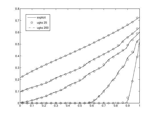
Figure 1: Kinetic regime (example 1): comparison between a reference solution and the UGKS (25 and 200 grid points). Results at times $t=0.1$, $0.4$, $1.0$, $1.6$ and $4$ ($\varepsilon=1$).

The results are plotted at times $t=0.1$, $0.4$, $1.0$, $1.6$, and $4$. We use 25 and 200 points for UGKS. The reference solution is obtained with 1000 points. In figure 1, we observe that the UGKS is very close to the reference solution, even with the coarse discretization for short times $t=0.1$ and $t=0.4$ (which is better than the AP schemes compared in [29]).

Example 2

Diffusion regime:

$$x\in[0,1],\qquad f_{L}(v)=1,\qquad f_{R}(v)=0,$$

$$\sigma=1,\qquad\alpha=0,\qquad G=0,\qquad\varepsilon=10^{-8}.$$

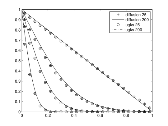
Figure 2: Diffusion regime (example 2): comparison between diffusion solution and the UGKS (25 and 200 grid points). Results at times $t=0.01$, $0.05$, $0.15$ and $2$ ($\varepsilon=10^{-8}$).

The results are plotted at times $t=0.01$, $0.05$, $0.15$ and $2$. We use 25 and 200 points for the UGKS. Here, the reference solution is obtained with the explicit discretization of the diffusion equation, since the kinetic equation cannot be solved by a the standard upwind scheme with such a small $\varepsilon$. In figure 2, we see that the UGKS and the diffusion solution are almost indistinguishable at any times for both coarse and fine discretizations.

Example 3

Intermediate regime with a variable scattering frequency and a source term:

$$x\in[0,1],\qquad f_{L}(v)=0,\qquad f_{R}(v)=0,$$

$$\sigma=1+(10x)^{2},\qquad\alpha=0,\qquad G=1,\qquad\varepsilon=10^{-2}.$$

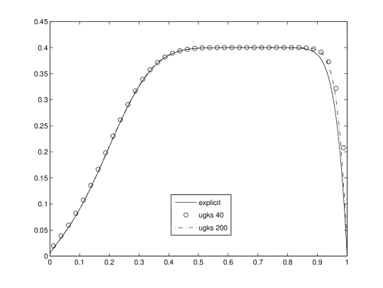
Figure 3: Intermediate regime with a variable scattering frequency and a source term (example 3): comparison between a reference solution and the UGKS (40 and 200 grid points).

The results are plotted at times $t=0.4$ with 40 and 200 points in figure 3. The reference solution is obtained with the explicit scheme using 20 000 points. We observe that the UGKS provides results that are very close to the reference solution, like the AP schemes compared in [29].

Example 4

Intermediate regime with a discontinuous scattering frequency and a source term. We take the following discontinuous values of $\sigma$:

$$x \in[0,0.1], x \in[0.1,0.5], x \in[0.5,1],$$

$$\sigma =1, \sigma =10, \sigma =100,$$

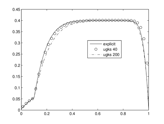
Figure 4: Intermediate regime with a discontinuous scattering frequency and a source term (example 4). Comparison between a reference solution and the UGKS (40 and 200 grid points): (top) first order schemes, (bottom) second order schemes.

while all the other parameters are like in example 3. In figure 4 (top), we show the behavior of the UGKS for coarse and thin meshes, as compared to a reference solution obtained by a fully explicit scheme with 20 000 cells. We observe that the UGKS gives results that are close to the reference solution. However, the result with the thin mesh is not as good as expected in the small to moderate scattering region ($x<0.4$). This is in fact due to the numerical dissipation induced by the first order reconstruction of $f(t_{n})$ around the cell interface (see (6)), since for small scattering, this gives a standard first order upwind scheme, which is known to be very diffusive.

This is confirmed by the following modification. We use a second order reconstruction with slope limiters to replace (6) by

$$f(t_{n},x,v)=\left\{\begin{split}&f_{i}^{n}+\frac{\Delta x}{2}\delta f^{n}_{i}\quad\text{ if }\quad x<x_{i+\frac{1}{2}}\\ &f_{i+1}^{n}-\frac{\Delta x}{2}\delta f^{n}_{i+1}\quad\text{ if }\quad x>x_{i+\frac{1}{2}},\end{split}\right.$$

where $\delta f^{n}_{i}$ is the slope computed with the MC limiter: $\delta f^{n}_{i}=\text{minmod}(\frac{f^{n}_{i+1}-f^{n}_{i-1}}{2\Delta x},\theta\frac{f^{n}_{i}-f^{n}_{i}}{\Delta x},$
$\theta\frac{f^{n}_{i+1}-f^{n}_{i}}{\Delta x})$ and $\theta=1.5$. Then, following the construction explained in section 2, we again obtain scheme (17)–(18), in which the additional term $B_{i+\frac{1}{2}}v(v\delta f^{n}_{i}\mathbbm{1}{v>0}+v\delta f^{n}_{i+1}\mathbbm{1}{v<0})$ must be added to the numerical flux given in (10), with

$$B(\Delta t,\varepsilon,\sigma,\alpha)=\frac{1}{\Delta t\varepsilon^{2}\nu}\Bigl{(}\Delta te^{-\nu\Delta t}-\frac{1}{\nu}\bigl{(}1-e^{-\nu\Delta t}\bigr{)}\Bigr{)}.$$

We also recompute the reference solution, still with 20 000 points, but with the same second order upwind reconstruction. We observe in figure 4 (bottom) that the UGKS results are now much closer to the reference solution, and that there is no visible difference between this solution and the UGKS with the thin mesh.

5.2 Comparison of different numerical boundary conditions

In this test, we compare the different numerical boundary conditions (BC) proposed for the UGKS in section 3.3 and 4.2. The BC given in (26) that ensures the stability of the scheme is called stabilized BC. We call corrected BC the one described in (29,30) that gives a correct boundary value in the diffusion limit. Finally, the blended BC is that defined in (31,32).

Example 5

First, we consider an intermediate regime with a non-isotropic boundary condition that generates a boundary layer of size $L=0.01$ at the left boundary:

$$x\in[0,1],\qquad f_{L}(v)=v,\qquad f_{R}(v)=0,$$

$$\sigma=1,\qquad\alpha=0,\qquad G=0,\qquad\varepsilon=10^{-2}$$

The results are plotted at times t = 0.4 with 25 and 200 points in figure 5 (see [29] for a comparison of other AP schemes on the same test case). The reference solution is obtained with the explicit scheme using 20 000 points. We also consider the diffusion scheme with 25 points, with a left boundary condition $\rho_{L}=17/24$ computed by formula (22) with the approximation $W(v)=3/2v^{2}+v$. With the coarse discretization, the boundary layer is of course not resolved. The stabilized BC is rather different from the reference solution in all the domain. At the contrary, we observe that the corrected and blended BC are very close to the reference solution inside the domain (far from the boundary).

With the fine discretization, the boundary layer is resolved: surprisingly, the corrected and blended BC are less close to the reference solution, while the stabilized version is now closer, even in the boundary layer. This fact is rather different from the other AP schemes already used for the this test (see [29]). We do not understand well the reason so far, but it might be linked to the fact that the coefficients $A,C,D$ of the UGKS depend in an intricate way on the numerical parameter $\Delta t$, $\Delta x$ and $\varepsilon$: for instance for a given small $\varepsilon$, $A$ and $D$ are closer to their limit value $0$ and $-1/\sigma$ for large $\Delta t$ and $\Delta x$ than for smaller values. See a similar observation in [34] about the high accuracy of the gas kinetic scheme (a macroscopic version of the UGKS) for under resolved cases.

Example 6

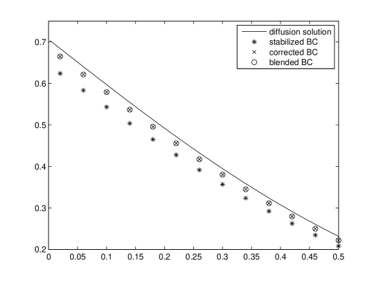
Figure 6: Boundary layer problem (example 6): stabilized, corrected, and blended boundary conditions for the UGKS are compared to the diffusion solution, $\varepsilon=10^{-4}$.

Then we take $\varepsilon=10^{-4}$ to be in a fully diffusion regime. The boundary layer is here very small and cannot be captured. The reference solution then is the solution of the diffusion equation, computed with $2000$ cells. The results are plotted at $t=0.4$ in figure 6. The comparison is almost the same as with $\varepsilon=10^{-2}$ for the coarse mesh: the stabilized BC gives a result which is not very accurate, while, as expected, the corrected and blended BC (which give the same results) are much closer to the diffusion solution. However, with the fine mesh, the corrected and blended BC now give no difference with the diffusion solution, while the stabilized BC is not accurate.

Example 7

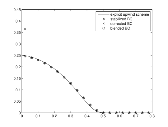
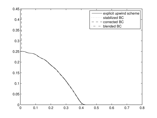
Figure 7: Free transport regime (example 7): stabilized, corrected, and blended boundary conditions for the UGKS are compared to the upwind explicit scheme, $\varepsilon=1$, $\sigma=0$.

Finally, in order to test our blended BC in all the regimes, we take $\varepsilon=1$ and $\sigma=1$, which is a purely transport regime (no collision). The results are plotted at times $t=0.4$ with 25 and 200 points in figure 7. Here, the comparison with a reference solution is difficult: indeed, it is well known that discrete ordinates methods in free transport regimes require many velocity points to be accurate. With a small number of velocities (like the 16 Gauss points we use here), the results show the well known “ray effect” that looks like several plateaus in the solution, and this phenomenon is stronger when the space mesh is refined. Consequently, we think it more interesting to compare the UGKS to a standard upwind explicit scheme with the same space resolution. As expected, we observe in figure 7 that both stabilized and blended BCs are very close to the standard scheme (for both coarse and refine space grids). At the contrary, the corrected BC (which is not consistent in the free transport regime) gives results that are far from the other schemes close to the boundary: it gives a numerical boundary layer at the left boundary that makes the solution much too large.

5.3 Implicit diffusion

Here, we illustrate the properties of the UGKS modified to recover an implicit scheme in the diffusion limit (see section 4.1). For this scheme, we take a time step defined by $\Delta t=\max(0.9\varepsilon\Delta x,cfl\Delta x)$–where $cfl$ depends on the problem (between $0.9$ and $0.1$)–such that we get $\Delta t=cfl\Delta x$ in the diffusion limit instead of $\Delta t=cfl\Delta x^{2}/2\mu$.

In figure 8, we compare this modified UGKS (denoted by UGKS-ID in the following) to the non-modified UGKS (denoted by UGKS-ED) and to the reference solutions for two unsteady cases. The data are those of example 1 (with a kinetic regime) and 2 (with a diffusion regime) shown in section 5.1. For example 1, we are in a kinetic regime where our modification is useless. However, with the fine mesh, the two UGKS give results that are very close. With the coarse mesh, there are some differences, but still quite small. For example 2, we are in a diffusion regime, where the UGKS-ID allows to take a time step which does not respect the parabolic CFL $\Delta t<\frac{\Delta x^{2}}{2\mu}$. Indeed, in the case of the fine mesh, while the UGKS-ID requires a time step of $3.37\,10^{-5}$, the UGKS-ED requires a time step of only $4.5\,10^{-2}$, which is $133$ times larger. In addition, we observe that both schemes give results that are very close. Of course, the results are different for the small times (the schemes are first order in time, hence a larger time step induces a larger numerical error), but we see that for longer times, both schemes give very close results. As expected, if the time step of the UGKS-ID is decreased, the difference with the UKGS-ED reduces too.

In figure 9, we compare our schemes for long time cases. The data are those of examples 3 (see section 5.1), and 5 (see section 5.2). We observe that for the coarse mesh, both schemes are very close. For example 3, the time step of UGKS-ID is 25 times as large as for UGKS-ED, while it is 16 times as large for example 5. For the fine mesh, UGKS-ID requires $cfl=0.1$ (it is unstable for larger CFL), and the time step is here 100 times as large as for UGKS-ED in example 3, and 10 times as large as for example 5. For example 5, UGKS-ID is different from the reference solution, but this difference is as large as the difference observed for UGKS-ED.

This study shows that the UGKS-ID can be efficiently used when the parabolic CFL condition is too much restrictive, with the same accuracy as the non-modified UGKS-ED.

6 Conclusion

In this paper, we have shown that the unified gas kinetic scheme, originally designed for rarefied gas dynamics problems, can be applied to other kinetic equations, like radiative transfer models. Moreover, the UGKS has been shown to be asymptotic preserving in the diffusion limit of such equations, as well as in the free transport regime. This scheme turns out to be an efficient multiscale method for kinetic problems, with a wide range of applications. In addition, we have shown that the UGKS can be simply modified to account for boundary layers and to obtain an implicit scheme in the diffusion limit. Finally, we have suggested an extension of the UGKS to general collision operator (in a non relaxation form) like that of neutron transport, that is still to be tested. This extension preserves the AP property of the method under some conditions.

It would be interesting to rigorously prove the stability of the UGKS, in particular to determine an explicit CFL condition: we believe that the energy method we proposed for another AP scheme in [30] could be applied. For practical applications, we would like to extend this work to multidimensional problems. This should not be difficult, since it has already been done in rarefied gas dynamics by Xu and Huang in [10].

Figure 5: Boundary layer problem (example 5): stabilized, corrected, and blended boundary conditions for the UGKS are compared to the explicit scheme (solid line with boundary layer) and the diffusion solution (solid straight line), $\varepsilon=10^{-2}$.

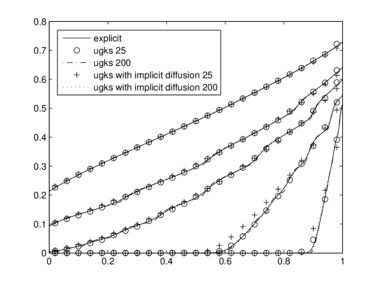
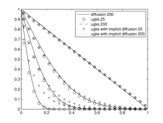
Figure 8: Comparison of the UGKS with/without implicit diffusion with a reference solution for unsteady cases. Data of of examples 1 (kinetic regime, top) and 2 (diffusion regime, bottom).

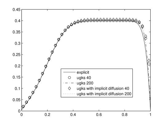
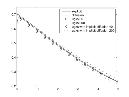
Figure 9: Comparison of the UGKS with/without implicit diffusion with a reference solution for long time cases. Data of of examples 3 (Intermediate regime with a variable scattering frequency and a source term, top) and 5 (intermediate regime with non-isotropic boundary conditions, bottom).

References

- [1] M. Bennoune, M. Lemou, and L. Mieussens. Uniformly stable numerical schemes for the Boltzmann equation preserving the compressible Navier-Stokes asymptotics. J. Comput. Phys., 227(8):3781–3803, 2008.
- [2] C. Buet, S. Cordier, B. Lucquin-Desreux, and S. Mancini. Diffusion limit of the Lorentz model: asymptotic preserving schemes. M2AN Math. Model. Numer. Anal., 36(4):631–655, 2002.
- [3] C. Buet, B. Després, and E. Franck. Design of asymptotic preserving finite volume schemes for the hyperbolic heat equation on unstructured meshes. Numerische Mathematik, 122:227–278, 2012.
- [4] J. A. Carrillo, T. Goudon, and P. Lafitte. Simulation of fluid and particles flows: asymptotic preserving schemes for bubbling and flowing regimes. J. Comput. Phys., 227(16):7929–7951, 2008.
- [5] J. A. Carrillo., T. Goudon, P. Lafitte, and F. Vecil. Numerical schemes of diffusion asymptotics and moment closures for kinetic equations. J. Sci. Comput., 36(1):113–149, 2008.
- [6] F. Filbet and S. Jin. A class of asymptotic-preserving schemes for kinetic equations and related problems with stiff sources. Journal of Computational Physics, 229(20):7625–7648, 2010.
- [7] L. Gosse. Transient radiative tranfer in the grey case: well-balanced and asymptotic-preserving schemes built on Case’s elementary solutions. Journal of Quantitative Spectroscopy and Radiative Transfer, 112:1995–2012, 2011.
- [8] L. Gosse and G. Toscani. An asymptotic-preserving well-balanced scheme for the hyperbolic heat equations. C. R. Math. Acad. Sci. Paris, 334(4):337–342, 2002.
- [9] L. Gosse and G. Toscani. Space localization and well-balanced schemes for discrete kinetic models in diffusive regimes. SIAM J. Numer. Anal., 41(2):641–658, 2003.
- [10] J.C. Huang, K. Xu, and P.B. Yu. A unified gas-kinetic scheme for continuum and rarefied flows ii: Multi-dimensional cases. Communications in Computational Physics, 3(3):662–690, 2012.
- [11] S. Jin. Efficient asymptotic-preserving (AP) schemes for some multiscale kinetic equations. SIAM J. Sci. Comput., 21(2):441–454, 1999.
- [12] S. Jin and C. D. Levermore. The discrete-ordinate method in diffusive regimes. Transport Theory Statist. Phys., 20(5-6):413–439, 1991.
- [13] S. Jin and C. D. Levermore. Fully discrete numerical transfer in diffusive regimes. Transport Theory Statist. Phys., 22(6):739–791, 1993.
- [14] S. Jin and C. D. Levermore. Numerical schemes for hyperbolic conservation laws with stiff relaxation terms. J. Comput. Phys., 126:449, 1996.
- [15] S. Jin and L. Pareschi. Discretization of the multiscale semiconductor Boltzmann equation by diffusive relaxation schemes. J. Comput. Phys., 161(1):312–330, 2000.
- [16] S. Jin and L. Pareschi. Asymptotic-preserving (AP) schemes for multiscale kinetic equations: a unified approach. In Hyperbolic problems: theory, numerics, applications, Vol. I, II (Magdeburg, 2000), volume 141 of Internat. Ser. Numer. Math., 140, pages 573–582. Birkhäuser, Basel, 2001.
- [17] S. Jin, L. Pareschi, and G. Toscani. Diffusive relaxation schemes for multiscale discrete-velocity kinetic equations. SIAM J. Numer. Anal., 35(6):2405–2439, 1998.
- [18] S. Jin, L. Pareschi, and G. Toscani. Uniformly accurate diffusive relaxation schemes for multiscale transport equations. SIAM J. Numer. Anal., 38(3):913–936, 2000.
- [19] A. Klar. An asymptotic-induced scheme for nonstationary transport equations in the diffusive limit. SIAM J. Numer. Anal., 35(3):1073–1094, 1998.
- [20] A. Klar. An asymptotic preserving numerical scheme for kinetic equations in the low Mach number limit. SIAM J. Numer. Anal., 36(5):1507–1527, 1999.
- [21] A. Klar. A numerical method for kinetic semiconductor equations in the drift-diffusion limit. SIAM J. Sci. Comput., 20(5):1696–1712, 1999.
- [22] A. Klar and C. Schmeiser. Numerical passage from radiative heat transfer to nonlinear diffusion models. Math. Models Methods Appl. Sci., 11(5):749–767, 2001.
- [23] A. Klar and A. Unterreiter. Uniform stability of a finite difference scheme for transport equations in diffusive regimes. SIAM J. Numer. Anal., 40(3):891–913, 2002.
- [24] P. Lafitte and G. Samaey. Asymptotic-preserving projective integration schemes for kinetic equations in the diffusion limit. SIAM Journal on Scientific Computing, 34(2):A579–A602, 2012.
- [25] A. W. Larsen and J. E. Morel. Asymptotic solutions of numerical transport problems in optically thick, diffusive regimes. II. J. Comput. Phys., 83(1):212–236, 1989.
- [26] A. W. Larsen, J. E. Morel, and W. F. Miller Jr. Asymptotic solutions of numerical transport problems in optically thick, diffusive regimes. J. Comput. Phys., 69(2):283–324, 1987.
- [27] M. Lemou. Relaxed micro-macro schemes for kinetic equations. C.R Acad. Sci., Serie I, 348(7-8):455–460, 2010.
- [28] M. Lemou and F. Méhats. Micro-macro schemes for kinetic equations including boundary layers. SIAM Journal on Numerical Analysis. to appear.
- [29] M. Lemou and L. Mieussens. A new asymptotic preserving scheme based on micro-macro formulation for linear kinetic equations in the diffusion limit. SIAM J. Sci. Comput., 31(1):334–368, 2008.
- [30] J. Liu and L. Mieussens. Analysis of an asymptotic preserving scheme for linear kinetic equations in the diffusion limit. SIAM Journal on Numerical Analysis, 48(4):1474–1491, 2010.
- [31] R. G. McClarren, T. M. Evans, R. B. Lowrie, and J. D. Densmore. Semi-implicit time integration for pn thermal radiative transfer. Journal of Computational Physics, 227:7561–7586, 2008.
- [32] G. Naldi and L. Pareschi. Numerical schemes for kinetic equations in diffusive regimes. Appl. Math. Lett., 11(2):29–35, 1998.
- [33] Sandra Pieraccini and Gabriella Puppo. Implicit–explicit schemes for bgk kinetic equations. Journal of Scientific Computing, 32:1–28, 2007.
- [34] Manuel Torrilhon and Kun Xu. Stability and consistency of kinetic upwinding for advection‚Äìdiffusion equations. IMA Journal of Numerical Analysis, 26(4):686–722, October 2006.
- [35] P. Wesseling. Principles of Computational Fluid Dynamics, volume 29 of Series: Springer Series in Computational Mathematics. Springer, 2001.
- [36] K. Xu. A gas-kinetic BGK scheme for the navier–stokes equations and its connection with artificial dissipation and godunov method. Journal of Computational Physics, 171(1):289 – 335, 2001.
- [37] K. Xu and J.-C. Huang. A unified gas-kinetic scheme for continuum and rarefied flows. J. Comput. Phys., 229:7747–7764, 2010.