Segmentation of the Poisson and negative binomial rate models: a penalized estimator

Abstract

We consider the segmentation problem of Poisson and negative binomial (i.e. overdispersed Poisson) rate distributions. In segmentation, an important issue remains the choice of the number of segments. To this end, we propose a penalized $\log$-likelihood estimator where the penalty function is constructed in a non-asymptotic context following the works of L. Birgé and P. Massart. The resulting estimator is proved to satisfy an oracle inequality. The performances of our criterion is assessed using simulated and real datasets in the RNA-seq data analysis context.

¹AgroParisTech/ INRA MIA 518, 16 rue Claude Bernard, 75231 Paris Cedex 05, France.
E-mail: alice.cleynen@agroparistech.fr
E-mail: emilie.lebarbier@agroparistech.fr

March 10, 2024

Mathematics subject classification 2010: primary 62G05, 62G07; secondary 62P10
Keywords and phrases: Density estimation; Change-points detection; Count data (RNA-seq); Poisson and negative binomial distributions; Model selection.

Introduction

We consider a multiple change-point detection setting for count datasets, which can be written as follows: we observe a finite sequence $\{y_{t}\}_{t\in\{1,\dots,n\}}$ realisation of independent variables $Y_{t}$. These variables are supposed to be drawn from a probability distribution $\mathcal{G}$ which depends on a set of parameters. Here two types of parameters are distinguished:

$$Y_{t}\sim\mathcal{G}(\theta_{t},\phi)=s(t),\;1\leq t\leq n,$$

where $\phi$ is a constant parameter while the $\theta$s are point-specific. In many contexts, we might want to consider that the $\theta$s are piece-wise constant and so subject to an unknown number $K-1$ of abrupt changes (for instance with climatic or financial data). Thus, we want to assume the existence of partition of $\{1,\dots,n\}$ into $K$ segments within which the observations follow the same distribution and between which observations have different distributions, i.e. $\theta$ is constant within a segment and differ from a segment to another. A motivating example is sequencing data analysis. For instance, the output of RNA-seq experiments is the number of reads (i.e. short portions of the genome) which first position maps to each location of a genome of reference. Supposing that we dispose of such a sequence, we expect to observe a stationarity in the amount of reads falling in different areas of the genome: expressed genes, intronic regions, etc. We wish to localize those regions that are biologically significant. In our context, we consider for $\mathcal{G}$ the Poisson and negative binomial distributions, adapted to RNA-seq experiment analysis [1].
Change-point detection problems are not new and many methods have been proposed in the literature. For count data-sets, [2] provide a detailed bibliography of methods in the particular case of the segmentation of the DNA sequences that includes Bayesian approaches, scan statistics, likelihood-ratio tests, binary segmentation and numerous other methods such as penalized contrast estimation procedures. In a Bayesian framework, [3] proposes to use an exact "ICL" criterion for the choice of $K$, while its approximation is computed in the constrained HMM approach of [4]. In this paper, we consider a penalized contrast estimation method which consists first, for every fixed $K$, in finding the best segmentation in $K$ segments by minimizing the contrast over all the partitions with $K$ segments, and then in selecting a convenient number of segments $K$ by penalizing the contrast. Choosing the number of segments, i.e. choosing a "good" penalty, is a crucial issue and not so easy. The most basic examples of penalty are the Akaike Information Criterion (AIC [5]) and the Bayes Information Criterion (BIC [6]) but these criteria are not well adapted in the segmentation context and tend to overestimate the number of change-points (see [7, 8] for theoretical explanations). In this particular context, some modified versions of these criteria have been proposed. For instance, [8, 9] have proposed modified versions of the BIC criterion (shown to be consistent) in the segmentation of Gaussian processes and DNA sequences respectively. However, these criteria are based on asymptotic considerations. In the last years there has been an extensive literature influenced by [10, 11] introducing non-asymptotic model selection procedures, in the sense that the size of the models as well as the size of the list of models are allowed to be large when $n$ is large. This penalized contrast procedure consists in selecting a model amongst a collection such that its performance is as close as possible to that of the best but unreachable model in terms of risk. This approach has been now considered in various function estimation contexts. In particular, [12] proposed a penalty for estimating the density of independent categorical variables in a least-squares framework, while [13, 14], or [15], focused on the estimation of the density of a Poisson process.
When the number of models is large, as in the case of an exhaustive search in segmentation problem, it can be shown that penalties which only depend on the number of parameters of each model, as for the classical criteria, are theoretically (and also practically) not adapted. This was suggested by [16, 7] who show that the penalty term needs to be well defined, and in particular needs to depend on the complexity of the list of models, i.e. the number of models having the same dimension. For this reason, following the work of [10] and in particular [17] in the density estimation framework, we consider a penalized $\log$-likelihood procedure to estimate the true distribution $s$ of a Poisson or negative binomial-distributed sequence $\mathbf{y}$. We prove that, up to a $\log n$ factor, the resulting estimator satisfies an oracle inequality.

The paper is organized as follows. The general framework is described in Section 1. More precisely, we present our proposed penalized maximum-likelihood estimator, the form of the penalty and give some non-asymptotic risk bounds for the resulting estimator. The studies of the two considered models (Poisson and negative binomial) are done in parallel along the paper. Some exponential bounds are derived in Section 2. A simulation study is performed to compare our proposed criterion with others and an application to the segmentation of RNA-seq data illustrates the procedure in Section 3. The proof of the main result is given in Section 4 for which the proofs of some intermediate results are given in the Appendix 5.

1 Model Selection Procedure

1.1 Penalized maximum-likelihood estimator

Let us denote by $m$ a partition of $[\![1,n]\!]$, $m=\{[\![1,\tau_{1}[\![,[\![\tau_{1},\tau_{2}[\![,\dots,[\![\tau_{k},n]\!]\}$ and by $\mathcal{M}_{n}$ a set of partitions of $[\![1,n]\!]$. In our framework we want to estimate the distribution $s$ defined by $s(t)=\mathcal{G}(\theta_{t},\phi),\,1\leq t\leq n$, and we consider the two following models:

$$\begin{array}[]{lll}\mathcal{G}(\theta_{t},\phi)&=\mathcal{P}(\lambda_{t})&(\mathcal{P})\\ \mathcal{G}(\theta_{t},\phi)&=\mathcal{NB}(p_{t},\phi)&(\mathcal{NB})\end{array}$$

In the ($\mathcal{NB}$) case, we suppose that the over-dispersion parameter $\phi$ is known. We define the collection of models :

Definition 1.1.

The collection of models associated to partition $m$ is $\mathcal{S}_{m}$ the set of distribution of sequences of length $n$ such that for each element $s_{m}$ of $\mathcal{S}_{m}$, for each segment $J$ of $m$, and for each $t$ in $J$, $s_{m}(t)=\mathcal{G}(\theta_{J},\phi)$:

$$\mathcal{S}_{m}=\left\{s_{m}\;|\;\forall J\in m,\;\forall t\in J,\;s_{m}(t)=\mathcal{G}(\theta_{J},\phi)\right\}.$$

We shall denote by $|m|$ the number of segments in partition $m$, and by $|J|$ the length of segment $J$.

We consider the log-likelihood contrast $\gamma(u)=\sum_{t=1}^{n}-\log\mathbf{P}_{u}(Y_{t})$, namely respectively for $u(t)=\mathcal{P}(\mu_{t})$ and $u(t)=\mathcal{NB}(q_{t},\phi)$,

$$\begin{array}[]{lll}\gamma(u)&=\sum_{t=1}^{n}\mu_{t}-Y_{t}\log(\mu_{t})+\log(Y_{t}!),&(\mathcal{P})\\ \gamma(u)&=\sum_{t=1}^{n}-\phi\log q_{t}-Y_{t}\log(1-q_{t})-\log\left(\frac{\Gamma(\phi+Y_{t})}{\Gamma(\phi)Y_{t}!}\right).&(\mathcal{NB})\end{array}$$

Then the minimal contrast estimator $\hat{s}_{m}$ of $s$ on the collection $\mathcal{S}_{m}$ is

$$\hat{s}_{m}=\arg\min_{u\in\mathcal{S}_{m}}\gamma(u),$$ (3)

so that, noting $\bar{Y}_{J}=\dfrac{\sum_{t\in J}Y_{t}}{|J|}$, for all $J\in m$ and $t\in J$

$$\hat{s}_{m}(t)=\mathcal{P}(\bar{Y}_{J})\,\text{for }(\mathcal{P})\quad\text{and}\;\hat{s}_{m}(t)=\mathcal{NB}\left(\dfrac{\phi}{\phi+\bar{Y}_{J}},\phi\right)\,\text{for }(\mathcal{NB}).$$ (4)

Therefore, for each partition $m$ of $\mathcal{M}_{n}$ we can obtain the best estimator $\hat{s}_{m}$ as in equation (4), and thus define a collection of estimators $\left\{(\hat{s}_{m})_{m\in\mathcal{M}_{n}}\right\}$. Ideally, we would wish to select the estimator $\hat{s}_{m(s)}$ amongst this collection with the minimum given risk. In the log-likelihood framework, it is natural to consider the Kullback-Leibler risk, with $K(s,u)=\mathbf{E}\left[\gamma(u)-\gamma(s)\right]$. In the following we note $\mathbf{E}$ and $\mathbf{P}$ the expectation and the probability under the true distribution $s$ respectively (otherwise the underlying distribution is mentioned). In our models, the Kullback-Leibler between distributions $s$ and $u$ can be developed into

$$\begin{array}[]{lll}K(s,u)&=\sum_{t=1}^{n}\left(\mu_{t}-\lambda_{t}-\lambda_{t}\log\dfrac{\mu_{t}}{\lambda_{t}}\right),&(\mathcal{P})\\ K(s,u)&=\phi\sum_{t=1}^{n}\log\left(\dfrac{p_{t}}{q_{t}}\right)+\dfrac{1-p_{t}}{p_{t}}\log\left(\dfrac{1-p_{t}}{1-q_{t}}\right).&(\mathcal{NB})\end{array}$$

Unfortunately, minimizing this risk requires the knowledge of the true distribution $s$, and is unreachable. We will therefore want to consider the estimator $\hat{s}_{\hat{m}}$ where $\hat{m}$ minimizes $\gamma(\hat{s}_{m})+pen(m)$ for a well-chosen function $pen$ (depending on the data). By doing so, we hope to select an estimator $\hat{s}_{\hat{m}}$ whose risk is as close as possible to the risk of $\hat{s}_{m(s)}=\arg\min_{m\in\mathcal{M}_{n}}\mathbf{E}_{s}[K(s,\hat{s}_{m})]$ in the sense that

$$\mathbf{E}[K(s,\hat{s}_{\hat{m}})]\leq C\,\mathbf{E}[K(s,\hat{s}_{m(s)})],$$

where $C$ is a nonnegative constant hopefully close to $1$. We therefore introduce the following definition:

Definition 1.2.

Let $\mathcal{M}_{n}$ be a collection of partitions of $[\![1,n]\!]$ constructed on a partition $m_{f}$ (i.e. $m_{f}$ is a refinement of every $m$ in $\mathcal{M}_{n}$). Given a nonnegative, increasing in the size of $m$ penalty function $pen$: $\mathcal{M}_{n}\rightarrow\mathbf{R}_{+}$, and choosing

$$\hat{m}=\arg\min_{m\in\mathcal{M}_{n}}\{\gamma(\hat{s}_{m})+pen(m)\},$$

we define the penalized maximum-likelihood estimator as $\hat{s}_{\hat{m}}$.

In the following Section we provide a choice of penalty function, and show that the resulting estimator satisfies an oracle inequality.

1.2 Choice of the penalty function

Main result

The following result shows that for an appropriate choice of the penalty function, we have a non-asymptotic risk bound for the penalized maximum-likelihood estimator.

Theorem 1.3.

Let $\mathcal{M}_{n}$ be a collection of partitions constructed on a partition $m_{f}$ such that there exist absolute positive constants $\rho_{min}$, $\rho_{max}$ and $\Gamma$ satisfying:

• $\forall t,\rho_{min}\leq\theta_{t}\leq\rho_{max}$ and

• $\forall J\in m_{f},|J|\geq\Gamma(\log(n))^{2}$.

Let $(L_{m})_{m\in\mathcal{M}_{n}}$ be some family of positive weights satisfying

$$\Sigma=\sum_{m\in\mathcal{M}_{n}}\exp(-L_{m}|m|)<+\infty.$$ (6)

Let $\beta>1/2$ in the Poisson case, $\beta>1/4$ in the negative binomial case. If for every $m\in\mathcal{M}_{n}$

$$pen(m)\geq\beta|m|\left(1+4\sqrt{L_{m}}\right)^{2},$$ (7)

then

$$\mathbf{E}\left[h^{2}(s,\hat{s}_{\hat{m}})\right] \leq C_{\beta}\inf_{m\in\mathcal{M}_{n}}\left\{K(s,\bar{s}_{m})+pen(m)\right\}+C(\phi,\Gamma,\rho_{min},\rho_{max},\beta,\Sigma),$$

with $C_{\beta}=\dfrac{(16\beta)^{1/3}}{(2\beta)^{1/3}-1}$ in model $(\mathcal{P})$ and $C_{\beta}=\dfrac{(4\beta)^{1/3}}{(4\beta)^{1/3}-1}$ in model $(\mathcal{NB})$.

We note $h^{2}(s,u)$ the squared Hellinger distance between distribution $s$ and $u$ and $\bar{s}_{m}$ is the projection of $s$ onto the collection $\mathcal{S}_{m}$ according to the Kullback-Leibler distance. The proof of this Theorem is given in Section 4.

Denoting $\bar{s}_{m}=\arg\min_{u\in\mathcal{S}_{m}}K(s,u)$, we have for $J\in m$ and $t\in J$,

$$\begin{array}[]{llll}\bar{s}_{m}(t)&=\mathcal{P}(\bar{\lambda}_{J})&\text{where}\;\bar{\lambda}_{J}=\dfrac{\sum_{t\in J}\lambda_{t}}{|J|}&(\mathcal{P})\\ \bar{s}_{m}(t)&=\mathcal{NB}(p_{J},\phi)&\text{where}\;p_{J}=\dfrac{|J|}{\sum_{t\in J}1/p_{t}}.&(\mathcal{NB})\end{array}$$ (10)

We remark that the risk of the penalized estimator $\hat{s}_{\hat{m}}$ is treated in terms of Hellinger distance instead of the Kullback-Leibler information. This is due to the fact that the Kullback-Leibler is possibly infinite, and so difficult to control. It is possible to obtain a risk bound in term of Kullback-Leibler if we have a uniform control of $||\log(s/\bar{s}_{m})||_{\infty}$ (see [18] for more explanation).

Choice of the weights $\{L_{m},m\in\mathcal{M}_{n}\}$.

The penalty function depends on the family $\mathcal{M}_{n}$ through the choice of the weights $L_{m}$ which satisfy (6). We consider for $\mathcal{M}_{n}$ the set of all possible partitions of $[\![1,n]\!]$ constructed on a partition $m_{f}$ which satisfies, for all segment $J$ in $m_{f}$, $|J|\geq\Gamma(\log n)^{2}$. Classically (see [19]) the weights are chosen as a function of the dimension of the model $s$, which is here $|m|$. The number of partitions of $\mathcal{M}_{n}$ having dimension $D$ being bounded by $n\choose{D}$, we have

$$\Sigma = \sum_{m\in\mathcal{M}_{n}}e^{L_{m}|m|}=\sum_{D=1}^{n}e^{-L_{D}D}Card\{m\in\mathcal{M}_{n},|m|=D\}$$

$$\leq \sum_{D=1}^{n}{n\choose{D}}e^{-L_{D}D}\leq\sum_{D=1}^{n}\left(\dfrac{en}{D}\right)^{D}e^{-L_{D}D}$$

$$\leq \sum_{D=1}^{n}e^{-D\left(L_{D}-1-\log\left(\dfrac{n}{D}\right)\right)}.$$

So with the choice $L_{D}=1+\kappa+\log\left(\dfrac{n}{D}\right)$ with $\kappa>0$, condition (6) is satisfied. Choosing, say $\kappa=0.1$, the penalty function can be chosen of the form

$$pen(m)=\beta|m|\left(1+4\sqrt{1.1+\log{\left(\frac{n}{|m|}\right)}}\right)^{2},$$ (11)

where $\beta$ is a constant to be calibrated.

Integrating this penalty in Theorem 1.3 leads to the following control:

$$\mathbf{E}\left[h^{2}(s,\hat{s}_{\hat{m}})\right]\leq C_{1}\inf_{m\in\mathcal{M}_{n}}\left\{K(s,\bar{s}_{m})+\beta|m|\left(1+4\sqrt{1.1+\log{\left(\frac{n}{|m|}\right)}}\right)^{2}\right\}+C(\phi,\Gamma,\rho_{min},\rho_{max},\beta,\Sigma)$$ (12)

The following proposition gives a bound on the Kullback-Leibler risk associated to $\hat{s}_{m}$:

Proposition 1.4.

Let $m$ be a partition of $\mathcal{M}_{n}$, $\hat{s}_{m}$ be the minimum contrast estimator and $\bar{s}_{m}$ be the projection of $s$ given by equations (4) and (10) respectively. Assume that there exists some positive absolute constants $\rho_{min}$, $\rho_{max}$ and $\Gamma$ such that $\forall t,\,\rho_{min}\leq\theta_{t}\leq\rho_{max}$ and $|J|\geq\Gamma(\log n)^{2}$. Then $\forall\varepsilon>0,\forall a>2$

$$K(s,\bar{s}_{m})-\dfrac{C_{1}(\phi,\Gamma,\rho_{min},\rho_{max},\varepsilon,a)}{n^{a/2-\alpha}}+C_{2}(\varepsilon)|m|\leq\mathbf{E}[K(s,\hat{s}_{m})],$$

where $\alpha<1$ is a constant that can be expressed according to $n$, $C_{2}(\varepsilon)=\dfrac{1}{2}\dfrac{1-\varepsilon}{(1+\varepsilon)^{2}}$ in the Poisson model $(\mathcal{P})$ and $C_{2}(\varepsilon)=\rho_{min}^{2}\dfrac{(1-\varepsilon)^{2}}{(1+\varepsilon)^{4}}$ in the negative binomial model $(\mathcal{NB})$.

The proof is given in appendix 5.1.

Combining proposition 1.4 and equation (12), we obtain the following oracle-type inequality:

Corollary 1.5.

Let $\mathcal{M}_{n}$ be a collection of partitions constructed on a partition $m_{f}$ such that there exist absolute positive constants $\rho_{min}$, $\rho_{max}$ and $\Gamma$ verifying:

• $\forall t,\rho_{min}\leq\theta_{t}\leq\rho_{max}$ and

• $\forall J\in m_{f},|J|\geq\Gamma(\log n)^{2}$.

There exists some absolute constant $C$ such that

$$\mathbf{E}\left[h^{2}(s,\hat{s}_{\hat{m}})\right] \leq C\log(n)\inf_{m\in\mathcal{M}_{n}}\left\{\mathbf{E}[K(s,\hat{s}_{m})]\right\}+C(\phi,\Gamma,\rho_{min},\rho_{max},\beta,\Sigma).$$

2 Exponential bounds

In order to prove Theorem 1.3, the general procedure in this model selection framework (see for example [19]) is the following: by definitions of $\hat{m}$ and $\hat{s}_{m}$ (see definition 1.2 and equation (3)), we have, $\forall m\in\mathcal{M}_{n}$

$$\gamma(\hat{s}_{\hat{m}})+pen(\hat{m})\leq\gamma(\hat{s}_{m})+pen(m)\leq\gamma(\bar{s}_{m})+pen(m).$$

Then, with $\bar{\gamma}(u)=\gamma(u)-\mathbf{E}[\gamma(u)]$,

$$K(s,\hat{s}_{\hat{m}})\leq K(s,\bar{s}_{m})+\bar{\gamma}(\bar{s}_{m})-\bar{\gamma}(\hat{s}_{\hat{m}})-pen(\hat{m})+pen(m).$$

The idea is therefore to control $\bar{\gamma}(\bar{s}_{m})-\bar{\gamma}(\hat{s}_{m^{\prime}})$ uniformly over $m^{\prime}\in\mathcal{M}_{n}$. This is more complicated when dealing with different models $m$ and $m^{\prime}$. Thus, following the work of [17] (see proof of Theorem 3.2, also recalled in [18]), we propose the following decomposition

$$\bar{\gamma}(\bar{s}_{m})-\bar{\gamma}(\hat{s}_{m^{\prime}})=\left(\bar{\gamma}(\bar{s}_{m^{\prime}})-\bar{\gamma}(\hat{s}_{m^{\prime}})\right)+\left(\bar{\gamma}(s)-\bar{\gamma}(\bar{s}_{m^{\prime}})\right)+\left(\bar{\gamma}(\bar{s}_{m})-\bar{\gamma}(s)\right),$$ (13)

and control each term separately. The first term is the most delicate to handle, and requires the introduction and the control of a chi-square statistic. The main difficulty here is the non-bounded characteristic of the objects we are dealing with. Indeed, in the classic density estimation context such as that of [17], the objects are probabilities which are bounded and so facilitate the direct use of concentration inequalities.
In our case, the chi-square statistic we introduce is denoted $\chi^{2}_{m}$ and defined by

$$\chi^{2}_{m}=\chi^{2}(\bar{s}_{m},\hat{s}_{m})=\sum_{J\in m}|J|\dfrac{(\bar{Y}_{J}-\bar{E}_{J})^{2}}{\bar{E}_{J}},$$ (14)

where we recall that $\bar{Y}_{J}=\dfrac{\sum_{t\in J}Y_{t}}{|J|}$ and use the notation $\bar{E}_{J}=\frac{E_{J}}{|J|}$ with $E_{J}=\sum_{t\in J}E_{t}$. Respectively for $(\mathcal{P})$ and $(\mathcal{NB})$, we have $E_{t}=\lambda_{t}$ and $E_{t}=\phi\frac{1-p_{t}}{p_{t}}$. The purpose is thus to control $\chi^{2}_{m}$ uniformly over $\mathcal{M}_{n}$. To this effect, we need to obtain an exponential bound of $Y_{J}=\sum_{t\in J}Y_{t}$ around its expectation. In Subsection 2.1, we recall a result of [15] that we use to derive an exponential bound for $\chi^{2}_{m}$ (Subsection 2.2).

2.1 Control of $Y_{J}$

First we recall a large deviation results established by [15] (lemma 3) that we apply in the Poisson and negative binomial frameworks.

Lemma 2.1.

Let $Y_{1},\dots,Y_{n}$ be $n$ independent centered random variables.

If $\log(\mathbf{E}[e^{zY_{i}}])\leq\kappa\dfrac{z^{2}\theta_{i}}{2(1-z\tau)}$ for all $z\in[0,1/\tau[$, and $1\leq i\leq n$, then

$$\mathbf{P}\left[\sum_{i=1}^{n}Y_{i}\geq\left(2\kappa x\sum_{i=1}^{n}\theta_{i}\right)^{1/2}+\tau x\right]\leq e^{-x}\ \text{for all }x>0.$$

If for $1\leq i\leq n$ and all $z>0$ $\log(\mathbf{E}[e^{-zY_{i}}])\leq\kappa z^{2}\theta_{i}/2$, then

$$\mathbf{P}\left[\sum_{i=1}^{n}Y_{i}\leq-\left(2\kappa x\sum_{i=1}^{n}\theta_{i}\right)^{1/2}\right]\leq e^{-x}\ \text{for all }x>0.$$

To apply this lemma we therefore need a majoration of $\log{\mathbf{E}\left[e^{z(Y_{t}-E_{t})}\right]}$ and $\log{\mathbf{E}\left[e^{-z(Y_{t}-E_{t})}\right]}$ for $z>0$.

Poisson case.

With $E_{t}=\lambda_{t}$, we have:

$$\log{\mathbf{E}\left[e^{z(Y_{t}-\lambda_{t})}\right]} = -z\lambda_{t}+\log{\mathbf{E}\left[e^{zY_{J}}\right]}=-z\lambda_{t}+\log{e^{(\lambda_{t}(e^{z}-1))}}=\lambda_{t}(e^{z}-z-1).$$

So

$$\log{\mathbf{E}\left[e^{z(Y_{t}-E_{t})}\right]}=E_{t}(e^{z}-z-1).$$

Negative binomial case.

In this case $E_{t}=\phi\frac{1-p_{t}}{p_{t}}$ and we have

$$\log\mathbf{E}\left(e^{z\left(Y_{t}-\phi\frac{1-p_{t}}{p_{t}}\right)}\right) = -z\phi\frac{1-p_{t}}{p_{t}}+\phi\log\frac{p_{t}}{1-(1-p_{t})e^{z}}\,\text{for }z\leq-\log(1-p_{t})$$

$$\leq \phi\left[\frac{1-p_{t}}{p_{t}}(-z)+\frac{1-p_{t}}{p_{t}}\frac{p_{t}}{1-(1-p_{t})e^{z}}(e^{z}-1)\right]$$

$$\leq \phi\left[\frac{1-p_{t}}{p_{t}}(-z)+\frac{1-p_{t}}{p_{t}}(e^{z}-1)\right]\leq\phi\frac{1-p_{t}}{p_{t}}(e^{z}-z-1).$$

So that in both cases,

$$\log{\mathbf{E}\left[e^{z(Y_{t}-E_{t})}\right]}\leq E_{t}(e^{z}-z-1).$$

Now using $e^{z}-z-1\leq\frac{z^{2}}{2(1-z)}$ for $z>0$ and $e^{z}-z-1\leq\frac{z^{2}}{2}$ for $z<0$, we have

$$\log{\mathbf{E}\left[e^{z(Y_{t}-E_{t})}\right]}\leq E_{t}\frac{z^{2}}{2(1-z)}\quad\text{and}\quad\log{\mathbf{E}\left[e^{-z(Y_{t}-E_{t})}\right]}\leq E_{t}\frac{z^{2}}{2}$$

Then,

$$P\left[Y_{J}-E_{J}\geq\sqrt{2xE_{J}}+x\right]\leq e^{-x},$$

or

$$P\left[Y_{J}-E_{J}\geq x\right]\leq e^{-\frac{x^{2}}{2(E_{J}+x)}}\ \ \text{and}\ \ P\left[|Y_{J}-E_{J}|\geq x\right]\leq 2e^{-\frac{x^{2}}{2(E_{J}+x)}}$$ (15)

2.2 Exponential bound for $\chi^{2}_{m}$

We first introduce the following set $\Omega_{m}$ defined by:

$$\Omega_{m}(\varepsilon)=\displaystyle\bigcap_{J\in m}\left\{\left|\dfrac{Y_{J}}{E_{J}}-1\right|\leq\varepsilon\right\},$$ (16)

for all $\varepsilon\in]0,1[$ and all segmentations $m$ such that each segment $J$ verifies $|J|\geq\Gamma(\log(n))^{2}$. This set has a large probability since we obtain

$$\mathbf{P}(\Omega_{m}(\varepsilon)^{C}) \leq \sum_{J\in m}\mathbf{P}\left(\left|Y_{J}-E_{J}\right|>\varepsilon E_{J}\right)\leq 2\sum_{J\in m}e^{-\frac{\varepsilon^{2}E_{J}}{2(1+\varepsilon)}}$$

$$\leq 2\sum_{J\in m}e^{-|J|\varepsilon^{\prime}f(\phi,\rho_{min})}\leq 2|m|\exp({-\varepsilon^{\prime}\Gamma f(\phi,\rho_{min})(\log(n))^{2}})$$

by applying equation (15) with $x=\varepsilon E_{J}$ and where $\varepsilon^{\prime}=\varepsilon^{2}/(2(1+\varepsilon))$ and $f(\phi,\rho_{min})>0$. Thus

$$\mathbf{P}(\Omega_{m}(\varepsilon)^{C}) \leq \dfrac{C(\phi,\Gamma,\rho_{min},\varepsilon,a)}{n^{a}},$$ (17)

with $a>2$.
The reason for introducing this set is double: in addition to enable the control of $\chi^{2}_{m}$ given by equation (14) on this restricted set, it allows us to link $K(\hat{s}_{m},\bar{s}_{m})$ to $V^{2}_{m}$ (see (23) for the control of the first term in the decomposition) and so to $\chi^{2}_{m}$, relation that we use to evaluate the risk of one model (see (25)).

Let $m_{f}$ be a partition of $\mathcal{M}_{n}$ such that $\forall J\in m_{f},|J|\geq\Gamma(\log(n))^{2}$ and assume that all considered partitions in $\mathcal{M}_{n}$ are constructed on this grid $m_{f}$. The following proposition gives an exponential bound for $\chi^{2}_{m}$ on the restricted event $\Omega_{m_{f}}(\epsilon)$.

Proposition 2.2.

Let $Y_{1},\ldots,Y_{n}$ be independent random variables with distribution $\mathcal{G}$ (Poisson or negative binomial distribution). Let $m$ be a partition of $\mathcal{M}_{n}$ with $|m|$ segments and $\chi^{2}_{m}$ the statistic given by (14). For any positive $x$, we have

$$\mathbf{P}\left[\chi^{2}_{m}\mathbf{1}_{\Omega_{m_{f}}(\epsilon)}\geq|m|+8(1+\varepsilon)\sqrt{x|{m}|}+4(1+\varepsilon)x\right] \leq e^{-x}.$$

Proof.

As in the density estimation framework, this quantity can be controlled using the Bernstein inequality. In our context, noting $\chi^{2}_{m}=\sum_{J\in m}Z_{J}$ where

$$Z_{J}=\frac{(Y_{J}-E_{J})^{2}}{E_{J}},$$

we need

• the calculation (or bounds) of the expectation of $\chi^{2}_{m}$:

  Poisson case

  $Y_{J}$ is distributed according to a Poisson distribution with parameter $\lambda_{J}$ so that

  $$\mathbf{E}\left[\chi^{2}_{m}\right]=|m|.$$ (18)

  Negative binomial case

  We have

  $$\mathbf{E}\left[\chi^{2}_{m}\right]=\sum_{J\in m}\frac{1}{|J|}\dfrac{\sum_{t\in J}Var(Y_{t})}{\phi\frac{1-p_{J}}{p_{J}}}=\sum_{J\in m}\frac{1}{|J|}\dfrac{\sum_{t\in J}\phi\frac{1-p_{t}}{p_{t}^{2}}}{\phi\frac{1-p_{J}}{p_{J}}},$$

  and thus

  $$|m|\leq\mathbf{E}\left[\chi^{2}_{m}\right]\leq\frac{1}{\rho_{min}}|m|.$$ (19)

• an upper bound of $\sum_{J\in m}\mathbf{E}[Z_{J}^{p}]$. For every $p\geq 2$ we have,

  $$\mathbf{E}\left[Z_{J}^{p}\mathbf{1}_{\Omega_{m_{f}}(\epsilon)}\right] = \frac{1}{E_{J}^{p}}\int_{0}^{+\infty}2p\ x^{2p-1}P\left[\left\{|Y_{J}-E_{J}|\geq x\right\}\cap\Omega_{m_{f}}(\epsilon)\right]dx$$

  $$\leq \frac{1}{E_{J}^{p}}\int_{0}^{\varepsilon E_{J}}2p\ x^{2p-1}P\left[|Y_{J}-E_{J}|\geq x\right]dx\text{.}$$

Using equation (15) and since $x\leq\varepsilon E_{J}$, we obtain the exponential bound $P\left[|Y_{J}-E_{J}|\geq x\right]\leq 2e^{-\frac{x^{2}}{2E_{J}(1+\varepsilon)}}.$

Therefore

$$\mathbf{E}\left[Z_{J}^{p}\mathbf{1}_{\Omega_{m_{f}}(\epsilon)}\right] \leq \frac{1}{E_{J}^{p}}\int_{0}^{\varepsilon E_{J}}4p\ x^{2p-1}e^{-\frac{x^{2}}{2E_{J}\left(1+\varepsilon\right)}}dx$$

$$\leq 4p\left(1+\varepsilon\right)^{p}\int_{0}^{+\infty}u^{2p-1}e^{-\frac{u^{2}}{2}}du$$

$$\leq 4p\left(1+\varepsilon\right)^{p}\int_{0}^{+\infty}\left(2t\right)^{p-1}e^{-t}dt$$

$$\leq 2^{p+1}p\left(1+\varepsilon\right)^{p}p!,$$

and

$$\sum_{J\in m}\mathbf{E}\left[Z_{J}^{p}\mathbf{1}_{\Omega_{m_{f}}(\epsilon)}\right]\leq 2^{p+1}p\left(1+\varepsilon\right)^{p}p!|m|\text{.}$$

Since $p\leq 2^{p-1}$,

$$\sum_{J\in m}\mathbf{E}\left[Z_{J}^{p}\mathbf{1}_{\Omega_{m_{f}}(\epsilon)}\right]\leq\frac{p!}{2}\times\left[2^{5}\left(1+\varepsilon\right)^{2}|m|\right]\times\left[4\left(1+\varepsilon\right)\right]^{p-2}.$$

We conclude by taking $v=2^{5}\left(1+\varepsilon\right)^{2}|m|$ and $c=4\left(1+\varepsilon\right)$ (see proposition 2.9 of [18] for the definition of the Bernstein’s inequality).

∎

3 Simulations and application

In the context of RNA-seq experiments, an important question is the (re)-annotation of the genome, that is, the precise localisation of the transcribed regions on the chromosomes. In an ideal situation, when considering the number of reads starting at each position, one would expect to observe a uniform coverage over each gene (proportional to its expression level), separated by regions of null signal (corresponding to non-transcribed regions of the genome). In practice however, those experiments tend to return very noisy signals that are best modelled by the negative binomial distribution.

In this Section, we first study the performance of the proposed penalized criterion by comparing it with others model selection criteria on a resampling dataset (Subsection 3.1). Then we provide an application on real data (Subsection 3.2). Since the penalty depends on the partition only through its size, the segmentation procedure is two-steps: first we estimate, for all number of segments $K$ between $1$ and $K_{max}$, the optimal partition with $K$ segments (i.e. construct the collection of estimators $\{\hat{s}_{K}\}_{1\leq K\leq K_{max}}$ where $\hat{s}_{K}=\arg\min_{\hat{s}_{m},m\in\mathcal{M}_{K}}\{\gamma(\hat{s}_{m})\}$). The optimal solution is obtained using a fast segmentation algorithm such as the Pruned Dynamic Programming Algorithm (PDPA, [20]) implemented for the Poisson and negative binomial losses or contrasts in the R package Segmentor3IsBack [21]. Then, we choose $K$ using our penalty function which requires the calibration of the constant $\beta$ that can be tuned according to the data by using the slope heuristic (see [7, 22]). Using the negative binomial distribution requires the knowledge of parameter $\phi$. We propose to estimate it using a modified version of the Jonhson and Kotz’s estimator [23].

3.1 Simulation study

We have assessed the performances of the proposed method (called Penalized PDPA) on a simulation scenario by comparing to five other procedures both its choice in the number of segments and the quality of the obtained segmentation using the Rand-Index $\mathcal{I}$. This index is defined as follows: let $C_{t}$ be the true index of the segment to which base $t$ belongs and let $\hat{C}_{t}$ be the corresponding estimated index, then

$$\mathcal{I}=\dfrac{2\sum_{t>s}\left[\mathbf{1}_{C_{t}=C_{s}}\mathbf{1}_{\hat{C}_{t}=\hat{C}_{s}}+\mathbf{1}_{C_{t}\neq C_{s}}\mathbf{1}_{\hat{C}_{t}\neq\hat{C}_{s}}\right]}{(n-1)(n-2)}.$$

The characteristics of the different algorithms are described in Table 1.

Algorithm	Dist	Complexity	Inference	Pen	Exact	Reference
Penalized PDPA	NB	$n\log n$	frequentist	external	exact	[21]
PDPA with BIC	NB	$n\log n$	frequentist	external	exact	[21]
Penalized PDPA	P	$n\log n$	frequentist	external	exact	[21]
PDPA with BIC	P	$n\log n$	frequentist	external	exact	[21]
PELT with BIC	P	$n$	frequentist	internal	exact	[24]
CART with BIC	P	$n\log n$	frequentist	external	heuristic	[25]
postCP with ICL	NB	$n$	frequentist	external	exact	[4]
EBS with ICL	NB	$n^{2}$	Bayesian	external	exact	[26]

Table 1: Properties of segmentation algorithms. The first column indicates the name of the algorithm and the criterion used for the choice of $K$. In the second column, NB stands for the negative binomial distribution and P for Poisson. The time of each algorithm is given (column "Complexity") and column "Exact" precises if the exact solution is reached.

The data we considered comes from a resampling procedure using real RNA-seq data. The original data, from a study by the Sherlock Genomics laboratory at Stanford University, is publicly available on the NCBIs Sequence Read Archive (SRA, url: http://www.ncbi.nlm.nih.gov/sra) with the accession number SRA048710. We created an artificial gene, inspired from the Drosophila inr-a gene, resulting in a $14$-segment signal with unregular intensities mimicking a differentially transcribed gene. $100$ datasets are thus created. Results are presented using boxplots in Figure 1. Because PELT’s estimate of $K$ averaged around $427$ segments, we did not show its corresponding boxplot.

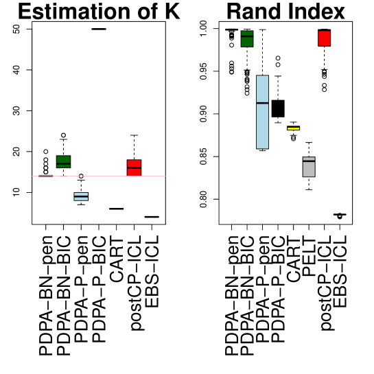
Figure 1: Estimation of K on resampled datasets. Left: boxplot of the estimation of $K$ on data-sets simulated by resampling on artificial gene Inr-a. PELT’s estimates average at $427$ segments and are not shown. The pink horizontal line indicates the true value of $K$. Right: boxplot of the Rand-Index values for the proposed estimators.

We can see that with the negative binomial distribution, not only do we perfectly recover the true number of segments, but our procedure outperforms all other approaches. Moreover, the impressive results in terms of Rand-Index prove that our choice of number of segments also leads to the almost perfect recovery of the true segmentation. However, the use of the Poisson loss leads to a constant underestimation of the number of segments, which is reflected on the Rand-Index values. This is due to the inappropriate choice of distribution (confirmed by the other algorithms implemented for the Poisson loss which perform worse than the others). It however underlines the need for the development of methods for the negative binomial distribution. Moreover, in terms of computational time, the fast algorithm [21] is in $\mathcal{O}(n\log n)$, allowing its use on long signals (such as a whole-genome analysis), even though it is not as fast as CART or PELT.

3.2 Segmentation of RNA-Seq data

We apply our proposed procedure for segmenting chromosome $1$ of the S. Cerevisiae (yeast) using RNA-Seq data from the Sherlock Laboratory at Stanford University [1] and publicly available from the NCBI’s Sequence Read Archive (SRA, url:http://www.ncbi.nlm.nih.gov/sra, accession number SRA048710). An existing annotation is available on the Saccharomyces Genome Database (SGD) at url:http://www.yeastgenome.org, which allows us to validate our results. The two distributions (Poisson and negative binomial) are considered here to show the difference.

In the Poisson distribution case, we select $106$ segments of which only $19$ are related to the SGD annotation. Indeed, as illustrated by Figure 2, $36$ of the segments have a length smaller than $10$: the Poisson loss is note adapted to this kind of data with high variability and it tends to select outliers as segment. On the contrary, we select $103$ segments in the negative binomial case most of which (all but $3$) surround known genes from the SGD. Figure 3 illustrates the result. However, almost none of those change-points correspond exactly to annotated boundaries. Discussion with biologists has increased our belief in the need for genome (re-)annotation using RNA-seq data, and in the validity of our approach.

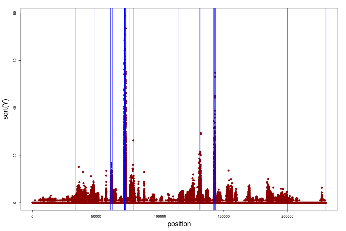
Figure 2: Segmentation of the yeast chromosome 1 using Poisson loss. Read-count are represented on a root-squared scale. The model selection procedure chooses $K=106$ segments.

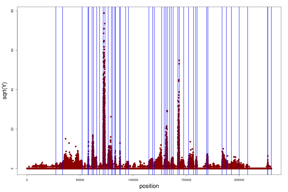
Figure 3: Segmentation of the yeast chromosome 1 using the negative binomial loss. The model selection procedure chooses $K=103$ segments, most of which surround genes given by the SGD annotation.

4 Proof of Theorem 1.3

Recall that we want to control the three terms in the decomposition given by (13). All the proofs of the different propositions are given in Section 5.

• The control the term $\bar{\gamma}(\hat{s}_{m^{\prime}})-\bar{\gamma}(\bar{s}_{m^{\prime}})$ is obtained with the following proposition where the set $\Omega_{1}(\xi)$ is defined by

  $$\Omega_{1}(\xi)=\bigcap_{m^{\prime}\in\mathcal{M}_{n}}\left\{\chi^{2}_{m^{\prime}}\mathbf{1}_{\Omega_{m_{f}}(\epsilon)}\leq|m^{\prime}|+8(1+\varepsilon)\sqrt{(L_{m^{\prime}}|m^{\prime}|+\xi)|m^{\prime}|}+4(1+\varepsilon)(L_{m^{\prime}}|m^{\prime}|+\xi)\right\}.$$

  Proposition 4.1.

  Let $m^{\prime}$ be a partition of $\mathcal{M}_{n}$. Then

  $$\left(\bar{\gamma}(\hat{s}_{m^{\prime}})-\bar{\gamma}(\bar{s}_{m^{\prime}})\right)\mathbf{1}_{\Omega_{m_{f}}(\epsilon)\cap\Omega_{1}(\xi)} \leq C(\varepsilon)\left[|m^{\prime}|+8(1+\varepsilon)\sqrt{(L_{m^{\prime}}|m^{\prime}|+\xi)|m^{\prime}|}\right.$$

  $$+\left.4(1+\varepsilon)(L_{m^{\prime}}|m^{\prime}|+\xi)\right]+\dfrac{1}{1+\varepsilon}K(\bar{s}_{m^{\prime}},\hat{s}_{m^{\prime}}),$$

  with $C(\varepsilon)=\frac{1}{2}\left(\frac{1+\varepsilon}{1-\varepsilon}\right)$ in the Poisson case and $C(\varepsilon)=\frac{1+\varepsilon}{4}$ in the negative binomial case.

• The control of the term $\bar{\gamma}(\bar{s}_{m})-\bar{\gamma}(s)$, or more precisely its expectation, is given by the following proposition:

  Proposition 4.2.

  $$|\mathbf{E}[(\bar{\gamma}(\bar{s}_{m})-\bar{\gamma}(s))\mathbf{1}_{\Omega_{m_{f}}(\epsilon)}]| \leq \frac{C(\phi,\Gamma,\rho_{min},\rho_{max},\varepsilon,a)}{n^{(a-1)/2}}.$$ (20)

• To control $\bar{\gamma}(s)-\bar{\gamma}(\bar{s}_{m^{\prime}})$, we use the following proposition which gives an exponential bound for $\bar{\gamma}(s)-\bar{\gamma}(u)$.

  Proposition 4.3.

  Let $s$ and $u$ be two distributions of a sequence $Y$. Let $\gamma$ be the log-likelihood contrast, $\bar{\gamma}(u)=\gamma(u)-\mathbf{E}[\gamma(u)]$, and $K(s,u)$ and $h^{2}(s,u)$ be respectively the Kullback-Leibler and the squared Hellinger distances between distributions $s$ and $u$. Then $\forall x>0$,

  $$\mathbf{P}\left[\bar{\gamma}(s)-\bar{\gamma}(u)\geq K(s,u)-2h^{2}(s,u)+2x\right] \leq e^{-x}.$$

  Applying it to $u=\bar{s}_{m^{\prime}}$ yields:

  $$\mathbf{P}\left[\bar{\gamma}(s)-\bar{\gamma}(\bar{s}_{m^{\prime}})\geq K(s,\bar{s}_{m^{\prime}})-2h^{2}(s,\bar{s}_{m^{\prime}})+2x\right] \leq e^{-x}.$$ (21)

  We then define $\Omega_{2}(\xi)=\bigcap_{m^{\prime}\in\mathcal{M}_{n}}\left\{\bar{\gamma}(s)-\bar{\gamma}(\bar{s}_{m^{\prime}})\leq K(s,\bar{s}_{m^{\prime}})-2h^{2}(s,\bar{s}_{m^{\prime}})+2(L_{m^{\prime}}|m^{\prime}|+\xi)\right\}$.

Let $\Omega(\varepsilon,\xi)=\Omega_{m_{f}}(\epsilon)\cap\Omega_{1}(\xi)\cap\Omega_{2}(\xi)$. Then, combining equation (21) and proposition 4.1, we get for $m^{\prime}=\hat{m}$,

$$(\bar{\gamma}(\bar{s}_{m})-\bar{\gamma}(\hat{s}_{\hat{m}}))\mathbf{1}_{\Omega(\epsilon,\xi)} = (\bar{\gamma}(s)-\bar{\gamma}(\bar{s}_{\hat{m}}))\mathbf{1}_{\Omega(\epsilon,\xi)}+(\bar{\gamma}(\bar{s}_{m})-\bar{\gamma}(s))\mathbf{1}_{\Omega(\epsilon,\xi)}+(\bar{\gamma}(\bar{s}_{\hat{m}})-\bar{\gamma}(\hat{s}_{\hat{m}}))\mathbf{1}_{\Omega(\epsilon,\xi)}$$

$$\leq \left[K(s,\bar{s}_{\hat{m}})-2h^{2}(s,\bar{s}_{\hat{m}})\right]\mathbf{1}_{\Omega(\epsilon,\xi)}+R\mathbf{1}_{\Omega(\epsilon,\xi)}+\dfrac{1}{1+\varepsilon}K(\bar{s}_{\hat{m}},\hat{s}_{\hat{m}})\mathbf{1}_{\Omega(\epsilon,\xi)}$$

$$+C(\varepsilon)\left[|\hat{m}|+8(1+\varepsilon)\sqrt{(L_{\hat{m}}|\hat{m}|+\xi)|\hat{m}|}+4(1+\varepsilon)(L_{\hat{m}}|\hat{m}|+\xi)\right]$$

$$+2L_{\hat{m}}|\hat{m}|+2\xi,$$

with $R=\bar{\gamma}(\bar{s}_{m})-\bar{\gamma}(s)$. So that

$$K(s,\hat{s}_{\hat{m}})\mathbf{1}_{\Omega(\epsilon,\xi)} \leq \left[K(s,\bar{s}_{\hat{m}})-2h^{2}(s,\bar{s}_{\hat{m}})\right]\mathbf{1}_{\Omega(\epsilon,\xi)}+\dfrac{1}{1+\varepsilon}K(\bar{s}_{\hat{m}},\hat{s}_{\hat{m}})\mathbf{1}_{\Omega(\epsilon,\xi)}$$

$$+C(\varepsilon)\left[|\hat{m}|+8(1+\varepsilon)\sqrt{(L_{\hat{m}}|\hat{m}|+\xi)|\hat{m}|}+4(1+\varepsilon)(L_{\hat{m}}|\hat{m}|+\xi)\right]$$

$$+K(s,\bar{s}_{m})\mathbf{1}_{\Omega(\epsilon,\xi)}+2L_{\hat{m}}|\hat{m}|+2\xi+R\mathbf{1}_{\Omega(\epsilon,\xi)}-pen(\hat{m})+pen(m).$$

And since

• $K(s,\hat{s}_{\hat{m}})=K(s,\bar{s}_{\hat{m}})+K(\bar{s}_{\hat{m}},\hat{s}_{\hat{m}})$ (see equation (22)),

• $K(s,u)\geq 2h^{2}(s,u)$ (see lemma 7.23 in [18]),

• $h^{2}(s,\hat{s}_{\hat{m}})\leq 2\left(h^{2}(s,\bar{s}_{\hat{m}})+h^{2}(\bar{s}_{\hat{m}},\hat{s}_{\hat{m}})\right)$ (using inequality $2ab\leq\kappa a^{2}+\kappa^{-1}b^{2}$ with $\kappa=1$),

$$\dfrac{\varepsilon}{1+\varepsilon}h^{2}(s,\hat{s}_{\hat{m}})\mathbf{1}_{\Omega(\epsilon,\xi)} \leq K(s,\bar{s}_{m})\mathbf{1}_{\Omega(\epsilon,\xi)}+R\mathbf{1}_{\Omega(\epsilon,\xi)}-pen(\hat{m})+pen(m)$$

$$+|\hat{m}|C(\varepsilon)\left[1+(1+\varepsilon)\left(8\sqrt{L_{\hat{m}}}+\varepsilon+4L_{\hat{m}}\right)\right]+2L_{\hat{m}}|\hat{m}|$$

$$+2\xi\left[1+C(\varepsilon)\left(8(1+\varepsilon)\dfrac{2}{\varepsilon}+4(1+\varepsilon)\right)\right].$$

But

$$C(\varepsilon)\left[1+(1+\varepsilon)\left(8\sqrt{L_{\hat{m}}}+\varepsilon+4L_{\hat{m}}\right)\right]+2L_{\hat{m}} \leq C(\varepsilon)\left[1+(1+\varepsilon)\left(\varepsilon+8\sqrt{L_{\hat{m}}}+8L_{\hat{m}}\right)\right]$$

$$\leq C_{2}(\varepsilon)\left[1+8\sqrt{L_{\hat{m}}}+8L_{\hat{m}}\right].$$

with $C_{2}(\varepsilon)=\dfrac{1}{2}\left(\dfrac{1+\varepsilon}{1-\varepsilon}\right)^{3}$ for $(\mathcal{P})$ and $C_{2}(\varepsilon)=\dfrac{1}{4}\left(1+\varepsilon\right)^{3}$ for $(\mathcal{NB})$. So we have

$$\dfrac{\varepsilon}{1+\varepsilon}h^{2}(s,\hat{s}_{\hat{m}})\mathbf{1}_{\Omega(\epsilon,\xi)} \leq K(s,\bar{s}_{m})\mathbf{1}_{\Omega(\epsilon,\xi)}+R\mathbf{1}_{\Omega(\epsilon,\xi)}-pen(\hat{m})+pen(m)$$

$$+|\hat{m}|C_{2}(\varepsilon)\left(1+4\sqrt{L_{\hat{m}}}\right)^{2}+2\xi\left[1+(1+\varepsilon)C(\varepsilon)\left(\dfrac{8}{\varepsilon}+2\right)\right].$$

By assumption, $pen(\hat{m})\geq\beta|\hat{m}|\left(1+4\sqrt{L_{\hat{m}}}\right)^{2}$. Choosing $\beta=C_{2}(\varepsilon)$ yields

$$h^{2}(s,\hat{s}_{\hat{m}})\mathbf{1}_{\Omega(\epsilon,\xi)} \leq C_{\beta}\left[K(s,\bar{s}_{m})\mathbf{1}_{\Omega(\epsilon,\xi)}+R\mathbf{1}_{\Omega(\epsilon,\xi)}+pen(m)\right]+\xi C(\beta).$$

Then, using propositions 4.2 and 4.1, we have $\mathbf{P}\left(\Omega_{1}(\xi)^{C}\right)\leq\sum_{m^{\prime}\in\mathcal{M}_{n}}e^{-L_{m^{\prime}}|m^{\prime}|+\xi}$ and $\mathbf{P}\left(\Omega_{2}(\xi)^{C}\right)\leq\sum_{m^{\prime}\in\mathcal{M}_{n}}e^{-L_{m^{\prime}}|m^{\prime}|+\xi}$. So that using hypothesis (6),

$$\mathbf{P}\left(\Omega_{1}(\xi)^{C}\cup\Omega_{2}(\xi)^{C}\right) \leq 2\sum_{m^{\prime}\in\mathcal{M}_{n}}e^{-L_{m^{\prime}}|m^{\prime}|+\xi}\leq 2\Sigma e^{-\xi},$$

and thus $\mathbf{P}\left(\Omega_{1}(\xi)\cap\Omega_{2}(\xi)\right)\geq 1-2\Sigma e^{-\xi}$. We now integrate over $\xi$, and using equation (20), we get with a probability larger than $1-2\Sigma e^{-\xi}$

$$\mathbf{E}\left[h^{2}(s,\hat{s}_{\hat{m}})\mathbf{1}_{\Omega_{m_{f}}(\epsilon)}\right] \leq C_{\beta}\left[K(s,\bar{s}_{m})+\frac{C(\phi,\Gamma,\rho_{min},\rho_{max},\beta,a)}{n^{(a-1)/2}}+pen(m)\right]+\Sigma C(\beta).$$

And since $\mathbf{E}\left[h^{2}(s,\hat{s}_{\hat{m}})\mathbf{1}_{\Omega_{m_{f}}(\epsilon)^{C}}\right]\leq\dfrac{C(\phi,\Gamma,\rho_{min},\rho_{max},\beta,a)}{n^{a-1}}$, we have

$$\mathbf{E}\left[h^{2}(s,\hat{s}_{\hat{m}})\right] \leq C_{\beta}\left[K(s,\bar{s}_{m})+pen(m)\right]+C^{\prime}(\phi,\Gamma,\rho_{min},\rho_{max},\beta,\Sigma).$$

Finally, by minimizing over $m\in\mathcal{M}_{n}$, we get

$$\mathbf{E}\left[h^{2}(s,\hat{s}_{\hat{m}})\right] \leq C_{\beta}\inf_{m\in\mathcal{M}_{n}}\left\{K(s,\bar{s}_{m})+pen(m)\right\}+C^{\prime}(\phi,\Gamma,\rho_{min},\rho_{max},\beta,\Sigma).$$

5 Appendices

5.1 Proof of proposition 1.4

Using Pythagore-type identity, we obtain the following decomposition (see for example [17]):

$$K(s,\hat{s}_{m})=K(s,\bar{s}_{m})+K(\bar{s}_{m},\hat{s}_{m}).$$ (22)

The objective is then to obtain a lower bound of $\mathbf{E}[K(\bar{s}_{m},\hat{s}_{m})]$ in the two considered distribution cases.

Poisson case

We have

$$K(\bar{s}_{m},\hat{s}_{m})=\sum_{J\in m}|J|\left(\bar{Y}_{J}-\bar{\lambda}_{J}-\bar{\lambda}_{J}\log\dfrac{\bar{Y}_{J}}{\bar{\lambda}_{J}}\right)=\sum_{J\in m}|J|\bar{\lambda}_{J}\Phi\left(\log{\dfrac{\bar{Y}_{J}}{\bar{\lambda}_{J}}}\right).$$

where $\Phi(x)=e^{x}-1-x$. Since $\dfrac{1}{2}x^{2}(1\wedge e^{x})\leq\Phi(x)\leq\dfrac{1}{2}x^{2}(1\vee e^{x})$, then on $\Omega_{m_{f}}(\epsilon)$, we have

$$\dfrac{1}{2}\log^{2}{\dfrac{\bar{Y}_{J}}{\bar{\lambda}_{J}}}\left(1\wedge\dfrac{\bar{Y}_{J}}{\bar{\lambda}_{J}}\right) \leq \Phi\left(\log{\frac{\bar{Y}_{J}}{\bar{\lambda}_{J}}}\right)\leq\dfrac{1}{2}\log^{2}{\dfrac{\bar{Y}_{J}}{\bar{\lambda}_{J}}}\left(1\vee\dfrac{\bar{Y}_{J}}{\bar{\lambda}_{J}}\right),$$

$$\frac{1-\varepsilon}{2}\log^{2}{\frac{\bar{Y}_{J}}{\bar{\lambda}_{J}}} \leq \Phi\left(\log{\frac{\bar{Y}_{J}}{\bar{\lambda}_{J}}}\right)\leq\frac{1+\varepsilon}{2}\log^{2}{\frac{\bar{Y}_{J}}{\bar{\lambda}_{J}}}.$$

So

$$\frac{1-\varepsilon}{2}V^{2}_{m} \leq K(\bar{s}_{m},\hat{s}_{m})\leq\frac{1+\varepsilon}{2}V^{2}_{m},$$ (23)

where

$$V^{2}_{m}=V^{2}(\bar{s}_{m},\hat{s}_{m}) = \sum_{J\in m}|J|\bar{\lambda}_{J}\log^{2}{\frac{\bar{Y}_{J}}{\bar{\lambda}_{J}}}=\sum_{J\in m}|J|\dfrac{(\bar{Y}_{J}-\bar{\lambda}_{J})^{2}}{\bar{\lambda}_{J}}\left(\dfrac{\log\frac{\bar{Y}_{J}}{\bar{\lambda}_{J}}}{\frac{\bar{Y}_{J}}{\bar{\lambda}_{J}}-1}\right)^{2}.$$ (24)

And using, for $x>0$, $\dfrac{1}{1\vee x}\leq\dfrac{\log x}{x-1}\leq\dfrac{1}{1\wedge x}$, we get, on $\Omega_{m_{f}}(\epsilon)$

$$\dfrac{1}{(1+\varepsilon)^{2}}\ \chi^{2}_{m}\leq V^{2}_{m}\leq\dfrac{1}{(1-\varepsilon)^{2}}\ \chi^{2}_{m}.$$ (25)

So

$$\dfrac{1-\varepsilon}{2(1+\varepsilon)^{2}}\ \chi^{2}_{m}\mathbf{1}_{\Omega_{m_{f}}(\epsilon)}\leq K(\bar{s}_{m},\hat{s}_{m})\mathbf{1}_{\Omega_{m_{f}}(\epsilon)}\leq\dfrac{1+\varepsilon}{2(1-\varepsilon)^{2}}\ \chi^{2}_{m}\mathbf{1}_{\Omega_{m_{f}}(\epsilon)}.$$

On one hand, $\mathbf{E}\left[\chi^{2}_{m}\right]=|m|$, and

$$\dfrac{1-\varepsilon}{2(1+\varepsilon)^{2}}|m|-\mathbf{E}\left[\chi^{2}_{m}\mathbf{1}_{\Omega_{m_{f}}(\epsilon)^{C}}\right]\leq\mathbf{E}\left[K(\bar{s}_{m},\hat{s}_{m})\mathbf{1}_{\Omega_{m_{f}}(\epsilon)}\right]\leq\dfrac{1+\varepsilon}{2(1-\varepsilon)^{2}}|m|.$$

Since $\chi^{2}_{m}\leq\frac{1}{\Gamma(\log{(n)})^{2}\rho_{min}}\sum_{J\in m}(Y_{J}-\lambda_{J})^{2}\leq\frac{1}{\Gamma(\log{(n)})^{2}\rho_{min}}\left(\sum_{t}Y_{t}-\sum_{t}\lambda_{t}\right)^{2}$, using Cauchy-Schwarz Inequality, we get

$$\mathbf{E}\left[\chi^{2}_{m}\mathbf{1}_{\Omega_{m_{f}}(\epsilon)^{C}}\right] \leq \frac{1}{\Gamma(\log{(n)})^{2}\rho_{min}}\left[3\left(\sum_{t}\lambda_{t}\right)^{2}+\sum_{t}\lambda_{t}\right]^{1/2}P(\Omega_{m_{f}}(\epsilon)^{C})^{1/2}$$

$$\leq C(\Gamma,\rho_{min},\rho_{max})\frac{n}{(\log{(n)})^{2}}P(\Omega_{m_{f}}(\epsilon)^{C})^{1/2}$$

$$\leq C(\Gamma,\rho_{min},\rho_{max})n^{\alpha}P(\Omega_{m_{f}}(\epsilon)^{C})^{1/2}$$

$$\leq \frac{C(\phi,\Gamma,\rho_{min},\rho_{max},\varepsilon,a)}{n^{a/2-\alpha}},$$

where $\alpha=1-2\frac{\log{(\log{(n)})}}{\log{(n)}}$, $n\geq 2$. For example, $\alpha=0.62$ for $n=10^{6}$.

On the other hand, using $\log{1/x}\geq 1-x$ for all $x>0$, $\mathbf{E}\left[K(\bar{s}_{m},\hat{s}_{m})\mathbf{1}_{\Omega_{m_{f}}(\epsilon)^{C}}\right]\geq 0$. Finally, we have

$$K(s,\bar{s}_{m})+\dfrac{1-\varepsilon}{2(1+\varepsilon)^{2}}|m|-\dfrac{C_{1}(\Gamma,\rho_{min},\rho_{max},\varepsilon,a)}{n^{a/2-\alpha}}\leq\mathbf{E}[K(s,\hat{s}_{m})],$$

Negative binomial case

We have $K(\bar{s}_{m},\hat{s}_{m})=\phi\sum_{J\in m}\dfrac{|J|}{p_{J}}h_{\frac{\phi}{\phi+\bar{Y}_{J}}}\left(p_{J}\right)$ and $\forall 0<a<1,\,h_{a}(x)\geq\dfrac{1-x}{1-a}\log^{2}\left(\dfrac{1-x}{1-a}\right)$.
Then on $\Omega_{m_{f}}(\epsilon)$

$$K(\bar{s}_{m},\hat{s}_{m}) \geq \phi\sum_{J\in m}\dfrac{|J|}{p_{J}}\dfrac{1-p_{J}}{\frac{\bar{Y}_{J}}{\phi+\bar{Y}_{J}}}\log^{2}\left(\dfrac{\frac{\bar{Y}_{J}}{\phi+\bar{Y}_{J}}}{1-p_{J}}\right).$$

Introducing

$$V^{2}_{m}=\sum_{J\in m}\phi|J|\dfrac{1-p_{J}}{p_{J}}\log^{2}\left(\dfrac{\frac{\bar{Y}_{J}}{\phi+\bar{Y}_{J}}}{1-p_{J}}\right),$$ (26)

we get

$$K(\bar{s}_{m},\hat{s}_{m})\geq V^{2}_{m},$$ (27)

and since $\bar{Y}_{J}-\phi\frac{1-p_{J}}{p_{J}}=\frac{\phi+\bar{Y}_{J}}{p_{J}}\left(\frac{\bar{Y}_{J}}{\phi+\bar{Y}_{J}}-(1-p_{J})\right)$, we have

$$V^{2}_{m} = \sum_{J\in m}|J|\left(\frac{\phi}{\phi+\bar{Y}_{J}}\right)^{2}\dfrac{\left(\bar{Y}_{J}-\phi\frac{1-p_{J}}{p_{J}}\right)^{2}}{\phi\frac{1-p_{J}}{p_{J}}}\left[\dfrac{\log\left(\dfrac{\frac{\bar{Y}_{J}}{\phi+\bar{Y}_{J}}}{1-p_{J}}\right)}{\dfrac{\frac{\bar{Y}_{J}}{\phi+\bar{Y}_{J}}}{1-p_{J}}-1}\right]^{2}.$$

And finally,

$$K(\bar{s}_{m},\hat{s}_{m})\mathbf{1}_{\Omega_{m_{f}}(\epsilon)} \geq \rho_{min}^{2}\dfrac{(1-\varepsilon)^{2}}{(1+\varepsilon)^{4}}\ \chi^{2}_{m}\mathbf{1}_{\Omega_{m_{f}}(\epsilon)}.$$

Moreover, on one hand we have $|m|\leq\mathbf{E}\left[\chi^{2}_{m}\right]\leq\frac{1}{\rho_{min}}|m|$. On the other hand, since $\chi^{2}_{m}\leq\frac{1}{\Gamma(\log{(n)})^{2}\phi(1-\rho_{max})}\left(\sum_{t}Y_{t}-\sum_{t}E_{t}\right)^{2}$, using Cauchy-Schwarz Inequality, we get

$$\mathbf{E}\left[\chi^{2}_{m}\mathbf{1}_{\Omega_{m_{f}}(\epsilon)^{C}}\right] \leq \frac{\left[\mathbf{E}\left(Y_{t}-E_{t}\right)^{4}+6\phi^{2}\sum_{(t,l),l\neq t}\frac{1-p_{t}}{p_{t}^{2}}\frac{1-p_{l}}{p_{l}^{2}}\right]^{1/2}}{\Gamma(\log{(n)})^{2}\phi(1-\rho_{max})}P(\Omega_{m_{f}}(\epsilon)^{C})^{1/2},$$

$$\leq C(\Gamma,\rho_{min},\rho_{max})n^{\alpha}P(\Omega_{m_{f}}(\epsilon)^{C})^{1/2},$$

$$\leq \frac{C(\phi,\Gamma,\rho_{min},\rho_{max},\varepsilon,a)}{n^{a/2-\alpha}},$$

where $\alpha=1-2\frac{\log{(\log{(n)})}}{\log{(n)}}$, $n\geq 2$. Finally, we have

$$K(s,\bar{s}_{m})+\rho_{min}^{2}\dfrac{(1-\varepsilon)^{2}}{(1+\varepsilon)^{4}}|m|-\dfrac{C(\phi,\Gamma,\rho_{min},\rho_{max},\varepsilon,a)}{n^{a/2-\alpha}}\leq\mathbf{E}[K(s,\hat{s}_{m})].$$

5.2 Proof of proposition 4.1

Poisson case

The term to be controlled is $\bar{\gamma}(\hat{s}_{m^{\prime}})-\bar{\gamma}(\bar{s}_{m^{\prime}})=\sum_{J\in m^{\prime}}|J|\left(\bar{Y}_{J}-\bar{\lambda}_{J}\right)\log\dfrac{\bar{Y}_{J}}{\bar{\lambda}_{J}}$. Using Cauchy-Schwarz inequality, we have

$$\bar{\gamma}(\bar{s}_{m^{\prime}})-\bar{\gamma}(\hat{s}_{m^{\prime}}) \leq \sqrt{\chi^{2}_{m^{\prime}}}\ \ \sqrt{V^{2}_{m^{\prime}}},$$

with $\chi_{m^{\prime}}^{2}$ and $V^{2}_{m^{\prime}}$ defined as in equations (14) and (24). Then, using equation (23)

$$\left(\bar{\gamma}(\bar{s}_{m^{\prime}})-\bar{\gamma}(\hat{s}_{m^{\prime}})\right)\mathbf{1}_{\Omega_{m_{f}}(\epsilon)} \leq \sqrt{\chi^{2}_{m^{\prime}}}\ \ \sqrt{\frac{2}{1-\varepsilon}K(\bar{s}_{m^{\prime}},\hat{s}_{m^{\prime}})},$$

and using $2ab\leq\kappa a^{2}+\kappa^{-1}b^{2}$ for all $\kappa>0$, we get

$$\left(\bar{\gamma}(\bar{s}_{m^{\prime}})-\bar{\gamma}(\hat{s}_{m^{\prime}})\right)\mathbf{1}_{\Omega_{m_{f}}(\epsilon)} \leq \dfrac{\kappa}{2}\chi^{2}_{m^{\prime}}+\frac{\kappa^{-1}}{1-\varepsilon}K(\bar{s}_{m^{\prime}},\hat{s}_{m^{\prime}}).$$ (28)

And with proposition 2.2, we get, for $\kappa=\dfrac{1+\varepsilon}{1-\varepsilon}=2C(\varepsilon)$,

$$\left(\bar{\gamma}(\hat{s}_{m^{\prime}})-\bar{\gamma}(\bar{s}_{m^{\prime}})\right)\mathbf{1}_{\Omega_{m_{f}}(\epsilon)\cap\Omega_{1}(\xi)}$$

$$\leq\dfrac{1+\varepsilon}{2(1-\varepsilon)}\left[|m^{\prime}|+8(1+\varepsilon)\sqrt{(L_{m^{\prime}}|m^{\prime}|+\xi)|m^{\prime}|}+4(1+\varepsilon)(L_{m^{\prime}}|m^{\prime}|+\xi)\right]+\dfrac{1}{1+\varepsilon}K(\bar{s}_{m^{\prime}},\hat{s}_{m^{\prime}}).$$

Negative binomial case

In this case we can write $\bar{\gamma}(\hat{s}_{m^{\prime}})-\bar{\gamma}(\bar{s}_{m^{\prime}})=\sum_{J\in m^{\prime}}|J|\left(\bar{Y}_{J}-\bar{E}_{J}\right)\log\dfrac{\frac{\bar{Y}_{J}}{\phi+\bar{Y}_{J}}}{1-p_{J}}$. Again, using Cauchy-Schwarz inequality, and with $\chi^{2}_{m}$ and $V^{2}_{m}$ defined by equations (14) and (26), we get

$$\bar{\gamma}(\bar{s}_{m^{\prime}})-\bar{\gamma}(\hat{s}_{m^{\prime}}) \leq \sqrt{\chi^{2}_{m^{\prime}}}\ \ \sqrt{V^{2}_{m^{\prime}}},$$

so that with equation (27) and $2ab\leq\kappa a^{2}+\kappa^{-1}b^{2}$ for all $\kappa>0$

$$\left(\bar{\gamma}(\bar{s}_{m^{\prime}})-\bar{\gamma}(\hat{s}_{m^{\prime}})\right)\mathbf{1}_{\Omega_{m_{f}}(\epsilon)} \leq \dfrac{\kappa}{2}\chi^{2}_{m^{\prime}}+\frac{\kappa^{-1}}{2}K(\bar{s}_{m^{\prime}},\hat{s}_{m^{\prime}}).$$ (29)

Finally, with proposition 2.2 and $\kappa=\dfrac{1+\varepsilon}{2}=2C(\varepsilon)$,

$$\left(\bar{\gamma}(\hat{s}_{m^{\prime}})-\bar{\gamma}(\bar{s}_{m^{\prime}})\right)\mathbf{1}_{\Omega_{m_{f}}(\epsilon)\cap\Omega_{1}(\xi)}$$

$$\leq\dfrac{1+\varepsilon}{4}\left[|m^{\prime}|+8(1+\varepsilon)\sqrt{(L_{m^{\prime}}|m^{\prime}|+\xi)|m^{\prime}|}+4(1+\varepsilon)(L_{m^{\prime}}|m^{\prime}|+\xi)\right]+\dfrac{1}{1+\varepsilon}K(\bar{s}_{m^{\prime}},\hat{s}_{m^{\prime}}).$$

5.3 Proof of proposition 4.2

Poisson case

Noting that $\mathbf{E}[(\bar{\gamma}(\bar{s}_{m})-\bar{\gamma}(s))\mathbf{1}_{\Omega_{m_{f}}(\epsilon)}]=-\mathbf{E}[(\bar{\gamma}(\bar{s}_{m})-\bar{\gamma}(s))\mathbf{1}_{\Omega_{m_{f}}(\epsilon)^{C}}]$, we have

$$|\mathbf{E}[(\bar{\gamma}(\bar{s}_{m})-\bar{\gamma}(s))\mathbf{1}_{\Omega_{m_{f}}(\epsilon)}]| \leq |\mathbf{E}[(\bar{\gamma}(\bar{s}_{m})-\bar{\gamma}(s))\mathbf{1}_{\Omega_{m_{f}}(\epsilon)^{C}}]|\leq\mathbf{E}[|(\bar{\gamma}(\bar{s}_{m})-\bar{\gamma}(s))|\mathbf{1}_{\Omega_{m_{f}}(\epsilon)^{C}}]$$

$$\leq \mathbf{E}\left[\left|\left(\sum_{J}\sum_{t}(Y_{t}-E_{t})\log{(\rho_{max}/\rho_{min})}\right)\right|\mathbf{1}_{\Omega_{m_{f}}(\epsilon)^{C}}\right]$$

$$\leq \log{(\rho_{max}/\rho_{min})}\times\mathbf{E}\left[\left|\sum_{t}(Y_{t}-E_{t})\right|\mathbf{1}_{\Omega_{m_{f}}(\epsilon)^{C}}\right]$$

$$\leq \log{(\rho_{max}/\rho_{min})}\times\left(\left[\mathbf{E}\left(\sum_{t}(Y_{t}-E_{t})\right)^{2}\right]^{1/2}\times\left(P(\Omega_{m_{f}}(\epsilon)^{C}\right)^{1/2}\right)$$

$$\leq \left(n\rho_{max}\right)^{1/2}\times\log{(\rho_{max}/\rho_{min})}\times(P(\Omega_{m_{f}}(\epsilon)^{C})^{1/2},$$

which concludes the proof.

Negative binomial case

Once again, $\mathbf{E}[(\bar{\gamma}(\bar{s}_{m})-\bar{\gamma}(s))\mathbf{1}_{\Omega_{m_{f}}(\epsilon)}]=-\mathbf{E}[(\bar{\gamma}(\bar{s}_{m})-\bar{\gamma}(s))\mathbf{1}_{\Omega_{m_{f}}(\epsilon)^{C}}]$, and

$$|\mathbf{E}[(\bar{\gamma}(\bar{s}_{m})-\bar{\gamma}(s))\mathbf{1}_{\Omega_{m_{f}}(\epsilon)}]| \leq |\mathbf{E}[(\bar{\gamma}(\bar{s}_{m})-\bar{\gamma}(s))\mathbf{1}_{\Omega_{m_{f}}(\epsilon)^{C}}]|\leq\mathbf{E}[|(\bar{\gamma}(\bar{s}_{m})-\bar{\gamma}(s))|\mathbf{1}_{\Omega_{m_{f}}(\epsilon)^{C}}]$$

$$\leq \mathbf{E}\left[\left|\left(\sum_{J}\sum_{t}\left(Y_{t}-\phi\frac{1-p_{t}}{p_{t}}\right)\log{(1/(1-\rho_{min}))}\right)\right|\mathbf{1}_{\Omega_{m_{f}}(\epsilon)^{C}}\right]$$

$$\leq \log{(1/(1-\rho_{min}))}\times\mathbf{E}\left[\left|\sum_{t}\left(Y_{t}-E_{t}\right)\right|\mathbf{1}_{\Omega_{m_{f}}(\epsilon)^{C}}\right]$$

$$\leq \left(n\phi\frac{1}{\rho_{min}^{2}}\right)^{1/2}\times\log{\frac{1}{1-\rho_{min}}}\times(P(\Omega_{m_{f}}(\epsilon)^{C})^{1/2}$$

which concludes the proof.

5.4 Proof of proposition 4.3

Using the Markov inequality $\mathbf{P}\left[\bar{\gamma}(s)-\bar{\gamma}(u)\geq b\right]\leq\inf_{a}\left[e^{-ab}\mathbf{E}\left(e^{a(\bar{\gamma}(s)-\bar{\gamma}(u))}\right)\right]$ with $a=\frac{1}{2}$, we get

$$\mathbf{P}\left[\bar{\gamma}(s)-\bar{\gamma}(u)\geq b\right] \leq \exp\left[-\frac{b}{2}+\log\mathbf{E}\left[\exp\left(\frac{1}{2}\left(\gamma(s)-\gamma(u)\right)+\frac{1}{2}\mathbf{E}\left[\gamma(u)-\gamma(s)\right]\right)\right]\right]$$

$$\leq \exp\left[-\frac{b}{2}+\frac{1}{2}K(s,u)+\log\mathbf{E}\left[\exp\left(-\frac{1}{2}\sum_{t}\log\mathbf{P}_{s}(X_{t}=Y_{t})+\log\mathbf{P}_{u}(X_{t}=Y_{t})\right)\right]\right]$$

$$\leq \exp\left[-\frac{b}{2}+\frac{1}{2}K(s,u)+\sum_{t}\log\mathbf{E}\sqrt{\frac{\mathbf{P}_{u}(X_{t}=Y_{t})}{\mathbf{P}_{s}(X_{t}=Y_{t})}}\right]$$

$$\leq \exp\left[-\frac{b}{2}+\frac{1}{2}K(s,u)+\sum_{t}\mathbf{E}\sqrt{\frac{\mathbf{P}_{u}(X_{t}=Y_{t})}{\mathbf{P}_{s}(X_{t}=Y_{t})}}-n\right]$$

$$\leq \exp\left[-\frac{b}{2}+\frac{1}{2}K(s,u)-h^{2}(s,u)\right]$$

where $\mathbf{P}_{s}=\mathbf{P}$ denote the probability under the distribution $s$. Thus

$$\mathbf{P}\left[\bar{\gamma}(s)-\bar{\gamma}(u)\geq K(s,u)-2h^{2}(s,u)+2x\right] \leq e^{-x}.$$

The authors wish to thank Stéphane Robin for more than helpful discussions on the statistical aspect and Gavin Sherlock for his insight on the biological applications.

References

- [1] Risso D, Schwartz K, Sherlock G, Dudoit S: GC-Content Normalization for RNA-Seq Data. BMC Bioinformatics 2011, 12:480.
- [2] Braun JV, Muller HG: Statistical Methods for DNA Sequence Segmentation. Statistical Science 1998, 13(2):142–162, [http://www.jstor.org/stable/2676755].
- [3] Biernacki C, Celeux G, Govaert G: Assessing a Mixture Model for Clustering with the Integrated Completed Likelihood. IEEE Trans. Pattern Anal. Machine Intel. 2000, 22(7):719–725.
- [4] Luong TM, Rozenholc Y, Nuel G: Fast estimation of posterior probabilities in change-point models through a constrained hidden Markov model. Arxiv preprint arXiv:1203.4394 under review.
- [5] Akaike H: Information Theory and Extension of the Maximum Likelihood Principle. Second international symposium on information theory 1973, :267–281.
- [6] Yao YC: Estimating the number of change-points via Schwarz’ criterion. Statistics & Probability Letters 1988, 6(3):181–189.
- [7] Birgé L, Massart P: Minimal penalties for Gaussian model selection. Probab. Theory Related Fields 2007, 138(1-2):33–73.
- [8] Zhang NR, Siegmund DO: A modified Bayes information criterion with applications to the analysis of comparative genomic hybridization data. Biometrics 2007, 63:22–32. [PMID: 17447926].
- [9] Braun JV, Braun RK, Muller HG: Multiple changepoint fitting via quasilikelihood, with application to DNA sequence segmentation. Biometrika 2000, 87(2):301–314, [http://www.jstor.org/stable/2673465].
- [10] Birgé L, Massart P: From model selection to adaptive estimation. In Festschrift for Lucien Le Cam, New York: Springer 1997:55–87.
- [11] Barron A, Birgé L, Massart P: Risk bounds for model selection via penalization. Probab. Theory Related Fields 1999, 113(3):301–413.
- [12] Akakpo N: Estimating a discrete distribution via histogram selection. ESAIM Probab. Statist. 2009, To appear.
- [13] Reynaud-Bouret P: Adaptive estimation of the intensity of inhomogeneous Poisson processes via concentration inequalities. Probab. Theory Related Fields 2003, 126:103–153.
- [14] Birgé L: Model selection for Poisson processes. In Asymptotics: particles, processes and inverse problems, Volume 55 of IMS Lecture Notes Monogr. Ser., Beachwood, OH: Inst. Math. Statist. 2007:32–64.
- [15] Baraud Y, Birgé L: Estimating the intensity of a random measure by histogram type estimators. Probab. Theory Related Fields 2009, 143(1-2):239–284.
- [16] Lebarbier E: Detecting multiple change-points in the mean of Gaussian process by model selection. Signal Processing 2005, 85(4):717–736.
- [17] Castellan G: Modified Akaike’s criterion for histogram density estimation. C. R. Acad. Sci., Paris, Sér. I, Math. 330 2000, 8:729–732.
- [18] Massart P: Concentration inequalities and model selection, Volume 1896 of Lecture Notes in Mathematics. Berlin: Springer 2007. [Lectures from the 33rd Summer School on Probability Theory held in Saint-Flour, July 6–23, 2003, With a foreword by Jean Picard].
- [19] Birgé L, Massart P: Gaussian model selection. J. Eur. Math. Soc. (JEMS) 2001, 3(3):203–268.
- [20] Rigaill G: Pruned dynamic programming for optimal multiple change-point detection. Arxiv:1004.0887 2010, [http://arxiv.org/abs/1004.0887].
- [21] Cleynen A, Koskas M, Rigaill G: A Generic Implementation of the Pruned Dynamic Programing Algorithm. Arxiv preprint arXiv:1204.5564 2012.
- [22] Arlot S, Massart P: Data-driven calibration of penalties for least-squares regression. J. Mach. Learn. Res. 2009, 10:245–279 (electronic), [http://www.jmlr.org/papers/volume10/arlot09a/arlot09a.pdf[pdf]].
- [23] Johnson N, Kemp A, Kotz S: Univariate Discrete Distributions. John Wiley & Sons, Inc. 2005.
- [24] Killick R, Eckley I: changepoint: An R package for changepoint analysis 2011.
- [25] Breiman L, Friedman J, Olshen R, Stone C: Classification and Regression Trees. Monterey, CA: Wadsworth and Brooks 1984.
- [26] Rigaill G, Lebarbier E, Robin S: Exact posterior distributions and model selection criteria for multiple change-point detection problems. Statistics and Computing 2012, 22:917–929.