Rubidium Rydberg linear macrotrimers

Abstract

We investigate the interaction between three rubidium atoms in highly excited ($58p$) Rydberg states lying along a common axis and calculate the potential energy surfaces (PES) between the three atoms. We find that three-body long-range potential wells exist in some of these surfaces, indicating the existence of very extended bound states that we label macrotrimers. We calculate the lowest vibrational eigenmodes and the resulting energy levels and show that the corresponding vibrational periods are rapid enough to be detected spectroscopically.

I Introduction

Ultracold Rydberg systems are a particularly interesting avenue of study. Translationally, the atoms are very slow, yet their internal energies are very high. The large excitation of a single electron leads to exaggerated atomic properties, such as long lifetimes, large cross sections, and very large polarizabilities Gallagher (1994), which can lead to strong interactions between Rydberg atoms Anderson et al. (1998); Mourachko et al. (1998). Such interactions have led to various applications in quantum information processes over the past decade (see Saffman et al. (2010) for a comprehensive review).

Another active area of research with Rydberg atoms is in the area of long-range “exotic molecules”. Such examples include the trilobite and butterfly states, so-called because of the resemblence of their respective wave functions to these creatures. First predicted in Greene et al. (2000), these quantum states were detected more recently in Bendowsky et al. (2009). Also of interest are the formation and detection of macroscopic Rydberg molecules. In Boisseau et al. (2002), it was first predicted that weakly bound macrodimers could be formed from the induced Van der Waals interactions of two Rydberg atoms. However, we have shown more recently Samboy et al. (2011); Samboy and Côté (2011) that larger, more stable dimers can be formed via the strong $\ell$-mixing of various Rydberg states. Recent measurements Overstreet et al. (2009) have shown signatures of such macrodimers using an ultracold sample of cesium Rydberg atoms.

More recently, the focus of study has moved toward few-body interactions, such as between atom-diatom interactions Byrd et al. (2009); Soldán et al. (2002); Parazzoli et al. (2011) and diatom-diatom interactions Zemke et al. (2010); Byrd et al. (2010). Coinciding with this shift, there have been proposals Rittenhouse et al. (2011); Rittenhouse and Sadeghpour (2010); Liu and Rost (2006); Liu et al. (2009) for many-body long-range interactions involving Rydberg atoms. However, these works focus on the interactions between one Rydberg atom and ground state atoms or molecules. In this paper, we describe the long-range interactions between three Rydberg atoms arranged along a common axis and provide calculations, which predict the existence of bound trimer states. Here, we also present the lowest vibrational energies of these bound states, calculated via the oscillation eigenmodes of the bound system.

II Three Body Interactions

In Samboy et al. (2011) and Samboy and Côté (2011), we predicted the existence of long-range rubidium Rydberg dimers by analyzing potential energy curves corresponding to the interaction energies between the two Rydberg atoms. In these works, we diagonalized an interaction Hamiltonian consisting of the long-range Rydberg-Rydberg interaction energy and atomic fine structure in the Hund’s case (c) basis set. Each molecular state in the basis was symmetrized with respect to the $D_{\infty h}$ symmetry of the homonuclear dimer.

In general, adding a third atom to the interaction picture will change the physical symmetry of the system. However, to simplify our calculations, we assume that three identical Rydberg atoms lie along a common ($z$-) axis (see Fig. 1(a)). This preserves the $D_{\infty h}$ symmetry and permits the use of much of the two-body physics on the three-body system. We analyzed this symmetry state for three Rb $58s$ atoms and three Rb $58p$ atoms and found that the $58p$ case exhibited examples of three-dimensional wells, indicating that the three atoms are bound in a linear chain.

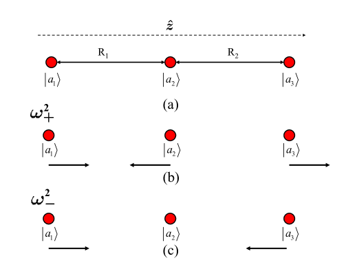
Figure 1: (Color online) (a) Three Rydberg atoms lie along a common $z$-axis. The distance between atoms 1 and 2 is represented by $R_{1}$ and the distance between atoms 2 and 3 is represented by $R_{2}$. Each atom is in state $|a_{i}\rangle$, defined in the text. Each bound macrotrimer has two eigenmodes of oscillation: (b) $\omega_{+}^{2}$ and (c) $\omega_{-}^{2}$ . (See text)

II.1 Basis States

Obtaining properly symmetrized basis functions for the three-atom case is very similar to that of the two-atom system (see Stanojevic et al. (2006)), but much more technically demanding. We construct the molecular wave functions from three free Rydberg atoms in respective states $|a_{1}\rangle\equiv|n_{1},\ell_{1},j_{1},m_{j_{1}}\rangle$, $|a_{2}\rangle\equiv|n_{2},\ell_{2},j_{2},m_{j_{2}}\rangle$, and $|a_{3}\rangle\equiv|a_{3},\ell_{3},j_{3},m_{j_{3}}\rangle$, where $n_{i}$ is the principal quantum number of atom $i$, $\ell_{i}$ is the orbital angular momentum of atom $i$, and $m_{j_{i}}$ is the projection of the total angular momentum $\vec{\boldsymbol{j}}_{i}=\vec{\boldsymbol{\ell}}_{i}+\vec{\boldsymbol{s}}_{i}$ of atom $i$ onto a quantization axis (chosen in the $z$-direction). As in the two-atom case, we assume that the three Rydberg atoms interact via long-range dipole-dipole and quadrupole-quadrupole couplings. Here, long-range indicates that the distance between each Rydberg atom is greater than the Le-Roy radius LeRoy (1974):

$$R_{LR}=2\,[\langle n_{1}\ell_{1}|r^{2}|n_{1}\ell_{1}\rangle^{1/2}+\langle n_{2}\ell_{2}|r^{2}|n_{2}\ell_{2}\rangle^{1/2}]\,\,,$$ (1)

such that there is no overlapping of the electron clouds. The properly symmetrized long-range three-atom wavefunctions take the form:

$$|a_{1};a_{2};a_{3}\rangle=\phantom{BLAHBLAH}$$

$$\dfrac{1}{\sqrt{6}}\left[\left(|a_{1}\rangle_{1}|a_{2}\rangle_{2}|a_{3}\rangle_{3}\right.\right. +|a_{2}\rangle_{1}|a_{3}\rangle_{2}|a_{1}\rangle_{3}$$

$$+\left.|a_{3}\rangle_{1}|a_{1}\rangle_{2}|a_{2}\rangle_{3}\right)$$ (2)

$$-P\left(|a_{1}\rangle_{1}|a_{3}\rangle_{2}|a_{2}\rangle_{3}\right. +|a_{2}\rangle_{1}|a_{1}\rangle_{2}|a_{3}\rangle_{3}$$

$$+\left.\left.|a_{3}\rangle_{1}|a_{2}\rangle_{2}|a_{1}\rangle_{3}\right)\right]\,\,,$$

where $P=p(-1)^{\ell_{1}+\ell_{2}+\ell_{3}}$, with $p=+1(-1)$ for gerade (ungerade) molecular states.

The basis set consists of the Rydberg molecular level being probed (e.g. $58p+58p+58p$), as well as all nearby asymptotes with significant coupling to this level and to each other. All of these states are properly symmetrized via Equation (II.1) according to their molecular symmetry $\Omega=m_{j_{1}}+m_{j_{2}}+m_{j_{3}}$. In this paper, we consider the $\Omega=1/2$ symmetry.

II.2 Interaction Hamiltonian

As in the two-atom case, we construct the interaction picture for the three-atom system by diagonalizing an interaction Hamiltonian in the properly symmetrized basis described in the previous subsection. The Hamiltonian consists of a three-body long-range Rydberg interaction energy and atomic fine structure, i.e. $H_{\rm{int}}=V_{3-\rm{body}}+H_{fs}$. Using the wave functions defined by Equation (II.1), we write the matrix elements of the Hamiltonian as the sums of multiple interactions. Each matrix element is defined as:

$$\langle a_{1};a_{2}; a_{3}|V_{3-\rm{body}}|b_{1};b_{2};b_{3}\rangle=$$

$$\frac{1}{6}\displaystyle\sum_{\begin{subarray}{c}i,j,k\\ i^{\prime},j^{\prime},k^{\prime}\end{subarray}}\langle a^{(1)}_{i}a^{(2)}_{j}a^{(3)}_{k}|V_{3-\rm{body}}|b^{(1)}_{i^{\prime}}b^{(2)}_{j^{\prime}}b^{(3)}_{k^{\prime}}\rangle$$ (3)

$$\times\left(\Theta_{C}+P_{a}\Theta_{A}\right)\left(\Theta_{C}+P_{b}\Theta_{A}\right)\,\,,$$

where each summation index is over the total number of atoms, i.e. from 1 to 3, $P$ is as before, we have defined

$$\begin{array}[]{ccc}&\Theta_{C}=\left\{\begin{array}[]{rl}-1&\mbox{for cyclic permutations}\\ 0&\mbox{for anti-cyclic permutations}\\ \end{array}\right.&\\ &&\\ &\mbox{and}&\\ &&\\ &\Theta_{A}=\left\{\begin{array}[]{rl}0&\mbox{for cyclic permutations}\\ -1&\mbox{for anti-cyclic permutations}\\ \end{array}\right.&\end{array}$$

and we have defined $|a^{(1)}_{i}a^{(2)}_{j}a^{(3)}_{k}\rangle\equiv|a_{i}\rangle_{1}|a_{j}\rangle_{2}|a_{k}\rangle_{3}$, etc. In the case that $|a_{1};a_{2};a_{3}\rangle=|b_{1};b_{2};b_{3}\rangle$ (i.e. along the diagonal of the matrix), the matrix element is given by:

$$\langle a_{1};a_{2};a_{3} |H_{\rm int}|a_{1};a_{2};a_{3}\rangle=$$

$$\langle a_{1};a_{2};a_{3}|V_{3-\rm{body}}|a_{1};a_{2};a_{3}\rangle+E_{123}\,\,,$$ (4)

with $E_{123}=E_{1}+E_{2}+E_{3}$, where $E_{k}=-\frac{1}{2}(n_{k}-\delta_{\ell_{k}})^{-2}$ are the atomic Rydberg energies with respective quantum defects $\delta_{\ell_{k}}$.

The long-range assumption assures that these are three free atoms interacting via long-range two-body potentials. That is, the transition element $\langle a^{(1)}_{i}a^{(2)}_{j}a^{(3)}_{k}|V_{3-\rm{body}}|b^{(1)}_{i^{\prime}}b^{(2)}_{j^{\prime}}b^{(3)}_{k^{\prime}}\rangle$ given in Equation (II.2) is defined as a sum of two-body interactions:

$$\langle a^{(1)}_{i}a^{(2)}_{j}a^{(3)}_{k}| V_{3-\rm{body}}|b^{(1)}_{i^{\prime}}b^{(2)}_{j^{\prime}}b^{(3)}_{k^{\prime}}\rangle=$$

$$\phantom{+}\;\,\langle a^{(1)}_{i}a^{(2)}_{j}|V_{L}(R_{12})|b^{(1)}_{i^{\prime}}b^{(2)}_{j^{\prime}}\rangle$$

$$+\langle a^{(2)}_{j}a^{(3)}_{k}|V_{L}(R_{23})|b^{(2)}_{j^{\prime}}b^{(3)}_{k^{\prime}}\rangle$$

$$+\langle a^{(1)}_{i}a^{(3)}_{k}|V_{L}(R_{13})|b^{(1)}_{i^{\prime}}b^{(3)}_{k^{\prime}}\rangle\,\,,$$ (5)

where $R_{\alpha\beta}$ is the nuclear separation between atoms $\alpha$ and $\beta$, and $L=1(2)$ for dipolar (quadrupolar) interactions. Since we are assuming that the three atoms lie along a common axis, each two-body interaction term $\langle a^{(\alpha)}_{i}a^{(\beta)}_{j}|V_{L}(R_{\alpha\beta})|b^{(\alpha)}_{i^{\prime}}b^{(\beta)}_{j^{\prime}}\rangle$ defines the long-range transition element between the two respective Rydberg atoms. Each transition element is given by Stanojevic et al. (2006); Samboy and Côté (2011):

$$\langle 1 2|V_{L}(R)|34\rangle=$$

$$(-1)^{L-1-m_{j_{\rm tot}}+j_{\rm tot}}\sqrt{\hat{\ell}_{1}\hat{\ell}_{2}\hat{\ell}_{3}\hat{\ell}_{4}\hat{j}_{1}\hat{j}_{2}\hat{j}_{3}\hat{j}_{4}}\;\dfrac{\mathcal{R}_{13}^{L}\;\mathcal{R}_{24}^{L}}{R^{2L+1}}$$

$$\times\left(\begin{array}[]{ccc}\ell_{1}&L&\ell_{3}\\ 0&0&0\\ \end{array}\right)\left(\begin{array}[]{ccc}\ell_{2}&L&\ell_{4}\\ 0&0&0\\ \end{array}\right)$$ (10)

$$\times\left\{\begin{array}[]{ccc}j_{1}&L&j_{3}\\ \ell_{3}&\frac{1}{2}&\ell_{1}\\ \end{array}\right\}\left\{\begin{array}[]{ccc}j_{2}&L&j_{4}\\ \ell_{4}&\frac{1}{2}&\ell_{2}\\ \end{array}\right\}$$ (15)

$$\times{\displaystyle\sum_{m=-L}^{L}}B_{2L}^{L+m}\left(\begin{array}[]{ccc}j_{1}&L&j_{3}\\ -m_{j_{1}}&m&m_{j_{3}}\\ \end{array}\right)$$ (18)

$$\times\left(\begin{array}[]{ccc}j_{2}&L&j_{4}\\ -m_{j_{2}}&-m&m_{j_{4}}\\ \end{array}\right)\,\,,$$ (21)

where $j_{\rm tot}=j_{1}+j_{2}+j_{3}+j_{4}$, $m_{j_{\rm tot}}=m_{j_{1}}+m_{j_{2}}+m_{j_{3}}+m_{j_{4}}$, $\hat{\ell}_{i}=2\ell_{i}+1$, $\hat{j}_{i}=2j_{i}+1$, and $\mathcal{R}_{ij}^{L}=\langle i|r^{L}|j\rangle$ is the radial matrix element.

III Potential Energy Surfaces

III.1 General Cases

We diagonalize the three-body Hamiltonian at successive values of $R_{1}$ and $R_{2}$, resulting in a series of potential energy surfaces (PES), where each surface corresponds to a different molecular asymptote in the basis. In each of the plots shown, $R_{1}$ represents the distance between atom 1 and atom 2, $R_{2}$ represents the distance between atom 2 and atom 3, both in $a_{0}$ (see Fig. 1(a)) and the energy is measured in GHz. The color scheme for the energy values is given in the scales to the right of each plot.

As a result of the large $\ell$-mixing that occurs between the Rydberg atoms, these surfaces have interesting topographies. For example, Figures 2 and 3 illustrate potential surfaces analogous to two-dimensional repulsive and attractive curves, respectively. The repulsive PES shown in Fig. 2 corresponds to the $|56p\frac{1}{2},\frac{1}{2};58p\frac{3}{2},-\frac{1}{2};60p\frac{3}{2},\frac{1}{2}\rangle$ state, while the attractive PES shown in Fig. 3 corresponds to the $|58s\frac{1}{2},\frac{1}{2};59s\frac{1}{2},-\frac{1}{2};57d\frac{5}{2},\frac{1}{2}\rangle$ state. We see that in both cases, the distance of the third atom has very little effect on the other two atoms: as either $R_{1}$ or $R_{2}$ is increased (while keeping the other distance fixed), the two stationary atoms consistently demonstrate an attractive/repulsive behavior.

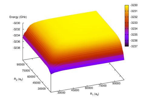
Figure 2: (Color online) Potential energy surface (PES) correlated to the $|56p\frac{1}{2},\frac{1}{2};58p\frac{3}{2},-\frac{1}{2};60p\frac{3}{2},\frac{1}{2}\rangle$ asymptotic state. This surface is analogous to a repsulsive potential curve for the two-body case: As the distance of either the first or last atom in the linear chain is increased, the two local atoms remain repulsed. The color scheme denotes the energy values given in GHz, with the scale presented to the right of the plot.

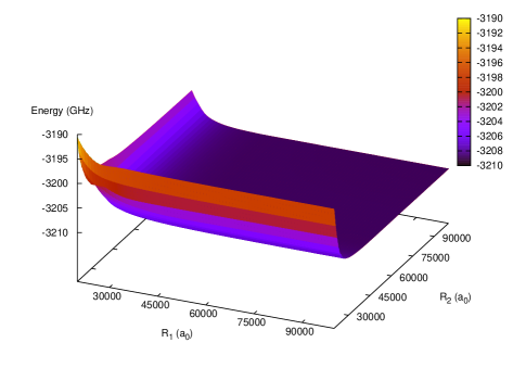
Figure 3: (Color online) Potential energy surface (PES) correlated to the $|58s\frac{1}{2},\frac{1}{2};59s\frac{1}{2},-\frac{1}{2};57d\frac{5}{2},\frac{1}{2}\rangle$ asymptotic state. This surface is analogous to an attractive potential curve for the two-body case: As the distance of either the first or last atom in the linear chain is increased, the two local atoms remain attracted. The color scheme denotes the energy values given in GHz, with the scale presented to the right of the plot.

Figure 4 illustrates another type of surface, in which there is a significant “ridge” running along one of the axes (in this case along the $R_{2}$ axis). Such a ridge indicates that the two local atoms (e.g. atom 1 and atom 2) form a bonded pair, existing even as atom 3 is moved away. This particular surface corresponds to the $|59s\frac{1}{2},-\frac{1}{2};55d\frac{3}{2},\frac{3}{2};58d\frac{3}{2},-\frac{1}{2}\rangle$ asymptotic state.

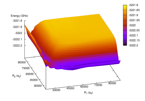
Figure 4: (Color online) Potential energy surface (PES) correlated to the $|59s\frac{1}{2},-\frac{1}{2};55d\frac{3}{2},\frac{3}{2};58d\frac{3}{2},-\frac{1}{2}\rangle$ asymptotic state. We note the “ridge” lying along the $R_{2}$ axis, which indicates that atom 1 and atom 2 are bound (see text). The color scheme denotes the energy values given in GHz, with the scale presented to the right of the plot.

III.2 Potential Wells

Although the surfaces highlighted in the previous section are interesting, ultimately we seek surfaces that illustrate potential wells, as these indicate bound three-atom systems. Upon separately investigating three excited $58s$ rubidium atoms and three excited $58p$ rubidium atoms, we found that in the case of the three excited $58p$ atoms, surface plots corresponding to various $58p+58p+58p$ asymptotes illustrated such (three-dimensional) potential wells. Specifically, wells were determined for the following states:

$|1\rangle\equiv|58p\frac{1}{2},\frac{1}{2};58p\frac{1}{2},\frac{1}{2};58p\frac{1}{2},-\frac{1}{2}\rangle$
$|2\rangle\equiv|58p\frac{1}{2},-\frac{1}{2};58p\frac{1}{2},-\frac{1}{2};58p\frac{3}{2},\frac{3}{2}\rangle$
$|3\rangle\equiv|58p\frac{1}{2},\frac{1}{2};58p\frac{3}{2},\frac{1}{2};58p\frac{3}{2},-\frac{1}{2}\rangle$
$|4\rangle\equiv|58p\frac{1}{2},-\frac{1}{2};58p\frac{3}{2},-\frac{1}{2};58p\frac{3}{2},\frac{3}{2}\rangle$
$|5\rangle\equiv|58p\frac{3}{2},-\frac{1}{2};58p\frac{3}{2},-\frac{1}{2};58p\frac{3}{2},\frac{3}{2}\rangle$  .

As an example, in Figure 5 we show the PES and the corresponding two-dimensional projection correlated to the $|1\rangle$ state, which demonstrates a potential well approximately 50-100 MHz deep. Due to the large equilibrium separations, e.g. $R_{1e}\sim 22$ 500 $a_{0}$ and $R_{2e}\sim 31$ 000 $a_{0}$, we label these bound states macrotrimers.

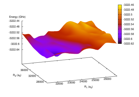
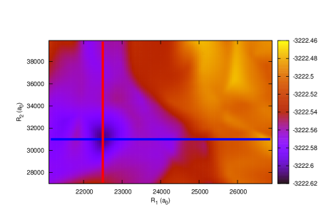
Figure 5: (Color online) Potential energy surface (top) and two-dimensional projection (bottom) correlated to the $|58p\frac{1}{2}\frac{1}{2};58p\frac{1}{2},\frac{1}{2};58p\frac{1}{2},-\frac{1}{2}\rangle$ asymptotic molecular state. The main feature of these plots is the three-dimensional well, centered at $R_{1e}=22$ 500 $a_{0}$ and $R_{2e}=31$ 000 $a_{0}$, indicating that the three Rydberg atoms are bound together in a linear chain (see text). The red (vertical) and blue (horizontal) lines imposed on the bottom plot are centered at the well minimum and indicate the cross-sections for which quadratic fits are performed (see Figure 6). The color scheme denotes the energy values given in GHz, with the scale presented to the right of each plot.

For the three-atom configuration shown in Figure 1(a), the (non-zero) oscillation modes can be calculated via:

$$\omega^{2}_{(\pm)}=\dfrac{(k_{1}+k_{2})\pm\sqrt{k_{1}^{2}-k_{1}k_{2}+k_{2}^{2}}}{m}\,\,,$$ (22)

where $k_{i}$ are “effective spring constants” that need to be calculated and $m$ is the mass of a single rubidium atom. In Figure 1(b) and (c), we show the physical description of each eigenmode. Panel (b) corresponds to the $\omega^{2}_{+}$ eigenvalue and shows that the two outer Rydberg atoms vibrate in the same direction, opposite to the inner atom’s direction of motion. Panel (c) corresponds to the $\omega^{2}_{-}$ eigenvalue and shows that the inner Rydberg atom is stationary while the outer two atoms oscillate in opposing directions.

Table 1: Characteristics of the polynomial fitting procedures for each trimer state $|i\rangle$ (see text), assumed to be quadratic. A two-dimensional cross-section was taken at the minimum of each well for both the $R_{1}$ and $R_{2}$ axes, where the well is centered ($R_{1e}$, $R_{2e}$). The $k_{\rm eff}$-values (in N/m) correspond to the numeric fitting along each respective axis. The well depth indicates the potential energy range for which the quadratic assumption is valid and for which the given $r^{2}$ goodness-of-fit values are appropriate.

State	Axis	$R_{e}(\times 10^{3}a_{0}$)	$k_{\rm eff}$ (N/m)	$r^{2}$-value	Depth (MHz)
$|1\rangle$	$R_{1}$	22.50	$8.37\times 10^{-11}$	0.9879	17.50
	$R_{2}$	31.00	$4.40\times 10^{-12}$	0.9926	16.60
$|2\rangle$	$R_{1}$	23.15	$3.85\times 10^{-11}$	0.9861	16.10
	$R_{2}$	33.10	$1.07\times 10^{-12}$	0.9781	77.50
$|3\rangle$	$R_{1}$	22.80	$2.55\times 10^{-11}$	0.9908	37.70
	$R_{2}$	34.60	$3.02\times 10^{-12}$	0.9892	21.30
$|4\rangle$	$R_{1}$	22.85	$4.63\times 10^{-11}$	0.9985	29.30
	$R_{2}$	31.50	$5.54\times 10^{-12}$	0.9943	05.80
$|5\rangle$	$R_{1}$	22.00	$6.87\times 10^{-11}$	0.9982	16.24
	$R_{2}$	31.70	$1.72\times 10^{-12}$	0.9992	11.94

To calculate the $k_{i}$ for Equation (22), we perform polynomial fits to two-dimensional cross sections of the potential wells along the $R_{1}$ and $R_{2}$ axes at each well’s minima (see Fig. 6). The deepest portions of each well can be modeled as a simple harmonic oscillator, and it is easily shown that the desired $k$-value equals the second derivative of these quadratic fits (with respect to the nuclear separation in that particular direction), i.e.

$$\left.k_{i}=\frac{d^{2}V}{dR_{i}^{2}}\right|_{R_{ie}}\,\,,$$ (23)

where $R_{ie}$ is the equilibrium separation along axis $R_{i}$. Table 1 summarizes the results of the polynomial fitting including the $k_{\rm eff}$-values, the goodness-of-fits ($r^{2}$ values) of the harmonic oscillator potentials, and the potential energy range for which the quadratic assumption is valid.

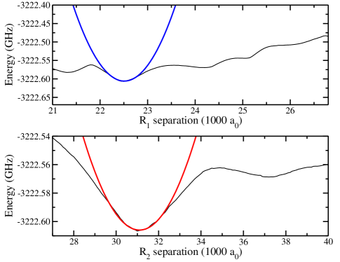
Figure 6: (Color online) Two-dimensional cross sections of the three dimensional surface shown in Figure 5 taken along the $R_{1}$ (top) and $R_{2}$ (bottom) axes at the well’s minimum. Each cross-section is fitted with a harmonic potential centered at the minimum. The results of these fits are summarized in Table 1.

Based on these properties, we use Equation (22) and the familiar $E=\hbar\omega(v+1/2)$ to find the oscillation energies in the deepest portions of the highlighted wells. Table 2 lists the vibrational energies of the first few bound states for each modal frequency, $\omega_{+}$ and $\omega_{-}$. We see that in each case, the energies defined by the $\omega_{+}$ frequency illustrate spacings of about 3-6 MHz, which are separated enough to be detected through spectroscopic means. The MHz energy values correspond to $\mu$s oscillation periods, which are rapid enough to allow for several oscillations during the lifetimes of these Rydberg atoms (roughly 500 $\mu$s for $n\sim 60$ Beterov et al. (2009)). The energies corresponding to the $\omega_{-}$ frequency are more closely spaced and demonstrate oscillation periods that are slower, but should still be able to be detected experimentally.

Table 2: Lowest vibrational levels and corresponding bound state energies for both oscillation frequencies of each trimer state $|i\rangle$ (see text). Energy_± represents the bound energies associated with $\omega_{\pm}$ and is measured from the bottom of the potential well.

State	$v$	Energy+ (MHz)	Energy- (MHz)
$|1\rangle$	0	02.71	00.62
	1	08.13	01.86
	2	13.55	03.11
	3	$-$	04.34
	$\vdots$	$\vdots$	$\vdots$
	12	$-$	15.53
$|2\rangle$	0	01.84	00.31
	1	05.51	00.92
	2	09.18	01.53
	3	12.86	02.14
	4	$-$	02.75
	$\vdots$	$\vdots$	$\vdots$
	25	$-$	15.60
$|3\rangle$	0	01.50	00.51
	1	04.48	01.54
	2	07.48	02.57
	3	10.47	03.60
	4	13.47	04.63
	5	16.46	05.66
	6	19.45	06.69
	7	$-$	07.72
	$\vdots$	$\vdots$	$\vdots$
	20	$-$	21.10
$|4\rangle$	0	02.02	00.70
	1	$-$	02.09
	2	$-$	03.49
	3	$-$	04.88
$|5\rangle$	0	02.46	00.39
	1	07.37	01.17
	2	$-$	01.94
	$\vdots$	$\vdots$	$\vdots$
	14	$-$	11.27

III.3 Other asymptotes

Of course, the potential wells described in section III.2 are not the only wells that exist. During the course of our analysis, we also found wells corresponding to various $|59s55d58d\rangle$ asymptotes; some examples of which are presented below. Although in principle these wells can be evaluated in the same amount of detail as was done for the $|58p58p58p\rangle$ wells in section III.2, we merely present visual evidence of their existence in this paper. Should these additional asymptotes lend themselves to specific experimental probing, then computing their respective energy levels would be of value. At this time, however, such evaluation is beyond the goals of this paper.

Figure 7: (Color online) Potential surface corresponding to the
$|59s\frac{1}{2}-\frac{1}{2};55d\frac{3}{2}\frac{1}{2};58d\frac{3}{2}\frac{1}{2}\rangle$ asymptotic state. The color scheme denotes the energy values given in GHz, with the scale presented to the right of the plot. This particular surface actually exhibits a few potential wells, the largest one being between 40-50 MHz deep.

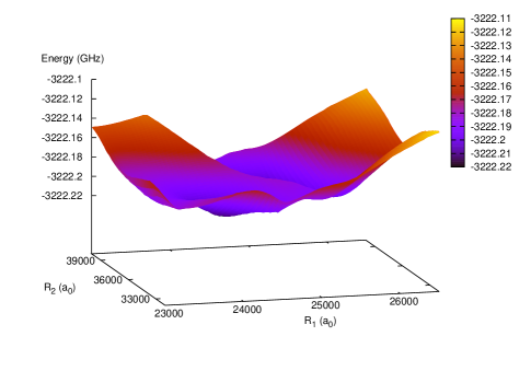
Figure 8: (Color online) Potential surface corresponding to the
$|59s\frac{1}{2}-\frac{1}{2};55d\frac{3}{2}-\frac{1}{2};58d\frac{3}{2}\frac{3}{2}\rangle$ asymptotic state. The color scheme denotes the energy values given in GHz, with the scale presented to the right of the plot. This particular surface exhibits two potential wells, each about 30-40 MHz deep.

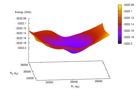
Figure 9: (Color online) Potential surface corresponding to the
$|59s\frac{1}{2}-\frac{1}{2};55d\frac{3}{2}\frac{3}{2};58d\frac{3}{2}-\frac{1}{2}\rangle$ asymptotic state. The color scheme denotes the energy values given in GHz, with the scale presented to the right of the plot. The well exhibited in this surface is 60-100 MHz deep.

IV Conclusions

The work presented in this letter demonstrates results for the $\Omega=1/2$ symmetry of $58p+58p+58p$ rubidium Rydberg atoms. During the course of our analysis, we also examined the surfaces corresponding to asymptotic states near the Rb $58s+58s+58s$ asymptote, but no potential wells were found for this case. The formalism could also be applied to the $58d+58d+58d$ case, but this would correspond to a large increase in computation time and thus, is outside the scope of the work shown in this paper. Due to an increased number of basis states for the triple $58d$ case, we would expect to find additional wells, however.

In addition, the methodology presented here can be applied to Rydberg states of other $\Omega$-symmetry values as well as to other alkali elements. The current literature regarding ultracold multi-body Rydberg physics involves one Rydberg atom interacting with multiple ground state atoms or a ground state molecule.

We seek to continue to analyze cases of Rydberg trimers for various alkali elements, asymptotes, and linear $\Omega$ symmetries, as well as exploring the energy levels corresponding to transverse (bending) modes of oscillation. Similarly, we seek to extend the theory to different molecular configurations, such as triangular systems. The detection of such trimer states could have applications in a variety of research areas, including quantum information processing and exotic, ultracold chemistry.

Furthermore, it might be possible to extend the linear chain to include $N$-Rydberg atoms, although this is purely speculative at this stage. Such investigations could prove fruitful in the advancement of ultracold multibody physics.