Robust subspace clustering

Abstract

Subspace clustering refers to the task of finding a multi-subspace representation that best fits a collection of points taken from a high-dimensional space. This paper introduces an algorithm inspired by sparse subspace clustering (SSC) [In IEEE Conference on Computer Vision and Pattern Recognition, CVPR (2009) 2790–2797] to cluster noisy data, and develops some novel theory demonstrating its correctness. In particular, the theory uses ideas from geometric functional analysis to show that the algorithm can accurately recover the underlying subspaces under minimal requirements on their orientation, and on the number of samples per subspace. Synthetic as well as real data experiments complement our theoretical study, illustrating our approach and demonstrating its effectiveness.

,
and t1Supported by a Benchmark Stanford Graduate Fellowship. t3Supported in part by AFOSR under Grant FA9550-09-1-0643 and by ONR under Grant N00014-09-1-0258 and by a gift from the Broadcom Foundation.

1 Introduction.

1.1 Motivation.

In many problems across science and engineering, a fundamental step is to find a lower-dimensional subspace which best fits a collection of points taken from a high-dimensional space; this is classically achieved via Principal Component Analysis (PCA). Such a procedure makes perfect sense as long as the data points are distributed around a lower-dimensional subspace, or expressed differently, as long as the data matrix with points as column vectors has approximately low rank. A more general model might sometimes be useful when the data come from a mixture model in which points do not lie around a single lower-dimensional subspace but rather around a union of low-dimensional subspaces. For instance, consider an experiment in which gene expression data are gathered on many cancer cell lines with unknown subsets belonging to different tumor types. One can imagine that the expressions from each cancer type may span a distinct lower-dimensional subspace. If the cancer labels were known in advance, one would apply PCA separately to each group but we here consider the case where the observations are unlabeled. Thus, the goal in such an example would be to separate gene expression patterns into different cancer types if possible. Finding the components of the mixture and assigning each point to a fitted subspace is called subspace clustering. Even when the mixture model holds, the full data matrix may not have low rank at all, a situation which is very different from that where PCA is applicable.

In recent years, numerous algorithms have been developed for subspace clustering and applied to various problems in computer vision/machine learning vidaltutorial and data mining parsons2004subspace . At the time of this writing, subspace clustering techniques are certainly gaining momentum as they begin to be used in fields as diverse as identification and classification of diseases montana , network topology inference highrankMC , security and privacy in recommender systems montanariSC , system identification sysID , hyper-spectral imaging hyperspectral , identification of switched linear systems masysid , ozay , and music analysis music to name just a few. In spite of all these interesting works, tractable subspace clustering algorithms either lack a theoretical justification, or are guaranteed to work under restrictive conditions rarely met in practice. (We note that although novel and often efficient clustering techniques come about all the time, establishing rigorous theory for such techniques has proven to be quite difficult. In the context of subspace clustering, Section 5 offers a partial survey of the existing literature.) Furthermore, proposed algorithms are not always computationally tractable. Thus, one important issue is whether tractable algorithms that can (provably) work in less than ideal situations—that is, under severe noise conditions and relatively few samples per subspace—exist.

Elhamifar and Vidal ehsanSSC have introduced an approach to subspace clustering, which relies on ideas from the sparsity and compressed sensing literature, please see also the longer version SSCalg which was submitted while this manuscript was under preparation. Sparse subspace clustering (SSC) ehsanSSC , SSCalg is computationally efficient since it amounts to solving a sequence of $\ell_{1}$ minimization problems and is, therefore, tractable. Now the methodology in ehsanSSC is mainly geared toward noiseless situations where the points lie exactly on lower-dimensional planes, and theoretical performance guarantees in such circumstances are given under restrictive assumptions. Continuing on this line of work, ourSSC showed that good theoretical performance could be achieved under broad circumstances. However, the model supporting the theory in ourSSC is still noise free.

This paper considers the subspace clustering problem in the presence of noise. We introduce a tractable clustering algorithm, which is a natural extension of SSC, and develop rigorous theory about its performance; see the results from Section 3.1. In a nutshell, we propose a statistical mixture model to represent data lying near a union of subspaces, and prove that in this model, the algorithm is effective in separating points from different subspaces as long as there are sufficiently many samples from each subspace and that the subspaces are not too close to each other. In this theory, the performance of the algorithm is explained in terms of interpretable and intuitive parameters such as (1) the values of the principal angles between subspaces, (2) the number of points per subspace, (3) the noise level and so on. In terms of these parameters, our theoretical results indicate that the performance of the algorithm is in some sense near the limit of what can be achieved by any algorithm, regardless of tractability.

1.2 Problem formulation and model.

We assume we are given data points lying near a union of unknown linear subspaces; there are $L$ subspaces $S_{1},S_{2},\ldots,S_{L}$ of $\mathbb{R}^{n}$ of dimensions $d_{1},d_{2},\ldots,d_{L}$. These together with their number are completely unknown to us. We are given a point set $\mathcal{Y}\subset\mathbb{R}^{n}$ of cardinality $N$, which may be partitioned as $\mathcal{Y}=\mathcal{Y}_{1}\cup\mathcal{Y}_{2}\cup\cdots\cup\mathcal{Y}_{L}$; for each $\ell\in\{1,\ldots,L\}$, $\mathcal{Y}_{\ell}$ is a collection of $N_{\ell}$ vectors that are “close” to subspace $S_{\ell}$. The goal is to approximate the underlying subspaces using the point set $\mathcal{Y}$. One approach is first to assign each data point to a cluster, and then estimate the subspaces representing each of the groups with PCA.

Our statistical model assumes that each point $\mathbf{y}\in\mathcal{Y}$ is of the form

$$\mathbf{y}=\mathbf{x}+\mathbf{z},$$ (1)

where $\mathbf{x}$ belongs to one of the subspaces and $\mathbf{z}$ is an independent stochastic noise term. We suppose that the inverse signal-to-noise ratio (SNR) defined as $\operatorname{\mathbb{E}}\|\mathbf{z}\|_{2}^{2}/\|\mathbf{x}\|_{\ell_{2}}^{2}$ is bounded above. Each observation is thus the superposition of a noiseless sample taken from one of the subspaces and of a stochastic perturbation whose Euclidean norm is about $\sigma$ times the signal strength so that $\operatorname{\mathbb{E}}\|z\|_{\ell_{2}}^{2}=\sigma^{2}\|x\|_{\ell_{2}}^{2}$. All the way through, we assume that

$$\sigma<\sigma^{\star}\quad\mbox{and}\quad\max_{\ell}{d_{\ell}}<c_{0}\frac{n}{{(\log N)}^{2}},$$ (2)

where $\sigma^{\star}<1$ and $c_{0}$ are fixed numerical constants. To remove any ambiguity, $\sigma$ is the noise level and $\sigma^{\star}$ the maximum value it can take on. The second assumption is here to avoid unnecessarily complicated expressions later on. While more substantial, the first is not too restrictive since it just says that the signal $\mathbf{x}$ and the noise $\mathbf{z}$ may have about the same magnitude. (With an arbitrary perturbation of Euclidean norm equal to two, one can move from any point $\mathbf{x}$ on the unit sphere to just about any other point.)

This is arguably the simplest model providing a good starting point for a theoretical investigation. For the noiseless samples $\mathbf{x}$, we consider the intuitive semirandom model introduced in ourSSC , which assumes that the subspaces are fixed with points distributed uniformly at random on each subspace. One can think of this as a mixture model where each component in the mixture is a lower-dimensional subspace. (One can extend the methods to affine subspace clustering as briefly explained in Section 2.)

1.3 What makes clustering hard?

Two important parameters fundamentally affect the performance of subspace clustering algorithms: (1) the distance between subspaces and (2) the number of samples on each subspace.

1.3.1 Distance/affinity between subspaces.

Intuitively, any subspace clustering algorithm operating on noisy data will have difficulty segmenting observations when the subspaces are close to each other. We of course need to quantify closeness, and Definition 1.2 captures a notion of distance or similarity/affinity between subspaces.

Definition 1.1.

The principal angles $\theta^{(1)},\ldots,\theta^{(d\wedge d^{\prime})}$ between two subspaces $S$ and $S^{\prime}$ of dimensions $d$ and $d^{\prime}$, are recursively defined by

$$\cos\bigl{(}\theta^{(i)}\bigr{)}=\max_{\mathbf{u}_{i}\in S}\max_{\mathbf{v}_{i}\in S^{\prime}}\frac{\mathbf{u}_{i}^{T}\mathbf{v}_{i}}{\|\mathbf{u}_{i}\|_{\ell_{2}}\|\mathbf{v}_{i}\|_{\ell_{2}}}$$

with the orthogonality constraints $\mathbf{u}_{i}^{T}\mathbf{u}_{j}=0$, $\mathbf{v}_{i}^{T}\mathbf{v}_{j}=0$, $j=1,\ldots,i-1$.

Alternatively, if the columns of $\mathbf{U}$ and $\mathbf{V}$ are orthobases for $S$ and $S^{\prime}$, then the cosine of the principal angles are the singular values of $\mathbf{U}^{T}\mathbf{V}$.

Definition 1.2.

The normalized affinity between two subspaces is defined by

$$\operatorname{aff}\bigl{(}S,S^{\prime}\bigr{)}=\sqrt{\frac{\cos^{2}\theta^{(1)}+\cdots+\cos^{2}\theta^{(d\wedge d^{\prime})}}{d\wedge d^{\prime}}}.$$

The affinity is a measure of correlation between subspaces. It is low when the principal angles are nearly right angles (it vanishes when the two subspaces are orthogonal) and high when the principal angles are small (it takes on its maximum value equal to one when one subspace is contained in the other). Hence, when the affinity is high, clustering is hard whereas it becomes easier as the affinity decreases. Ideally, we would like our algorithm to be able to handle higher affinity values—as close as possible to the maximum possible value.

There is a statistical description of the affinity which goes as follows: sample independently two unit-normed vectors $\mathbf{x}$ and $\mathbf{y}$ uniformly at random from $S$ and $S^{\prime}$. Then

$$\operatorname{\mathbb{E}}\bigl{\{}\bigl{(}\mathbf{x}^{T}\mathbf{y}\bigr{)}^{2}\bigr{\}}\propto\bigl{\{}\operatorname{aff}\bigl{(}S,S^{\prime}\bigr{)}\bigr{\}}^{2},$$

where the constant of proportionality is $d\vee d^{\prime}$. Having said this, there are of course other ways of measuring the affinity between subspaces; for instance, by taking the cosine of the first principal angle. We prefer the definition above as it offers the flexibility of allowing for some principal angles to be small or zero. As an example, suppose we have a pair of subspaces with a nontrivial intersection. Then $|\cos\theta^{(1)}|=1$ regardless of the dimension of the intersection whereas the value of the affinity would depend upon this dimension.

1.3.2 Sampling density.

Another important factor affecting the performance of subspace clustering algorithms has to do with the distribution of points on each subspace. In the model we study here, this essentially reduces to the number of points that lie on each subspace.

Definition 1.3.

The sampling density $\rho$ of a subspace is defined as the number of samples on that subspace per dimension. In our multi-subspace model, the density of $S_{\ell}$ is, therefore, $\rho_{\ell}=N_{\ell}/d_{\ell}$.

One expects the clustering problem to become easier as the sampling density increases. Obviously, if the sampling density of a subspace $S$ is smaller than one, then any algorithm will fail in identifying that subspace correctly as there are not sufficiently many points to identify all the directions spanned by $S$. Hence, we would like a clustering algorithm to be able to operate at values of the sampling density as low as possible, that is, as close to one as possible.

2 Robust subspace clustering: Methods and concepts.

This section introduces our methodology through heuristic arguments confirmed by numerical experiments while proven theoretical guarantees about the first step of algorithm follow in Section 3. From now on, we arrange the $N$ observed data points as columns of a matrix $\mathbf{Y}=[\mathbf{y}_{1},\ldots,\mathbf{y}_{N}]\in\mathbb{R}^{n\times N}$. With obvious notation, $\mathbf{Y}=\mathbf{X}+\mathbf{Z}$.

2.1 The normalized model.

In practice, one may want to normalize the columns of the data matrix so that for all $i$, $\|\mathbf{y}_{i}\|_{\ell_{2}}=1$ [R-code snippet for renormalizing a data point $y$ is: y <-y/sqrt(sum(y${}\wedge{}$2))]. Since with our SNR assumption, we have $\|\mathbf{y}\|_{\ell_{2}}\approx\|\mathbf{x}\|_{\ell_{2}}\sqrt{1+\sigma^{2}}$ before normalization, then after normalization:

$$\mathbf{y}\approx\frac{1}{\sqrt{1+\sigma^{2}}}(\mathbf{x}+\mathbf{z}),$$

where $\mathbf{x}$ is unit-normed, and $\mathbf{z}$ has i.i.d. random Gaussian entries with variance $\sigma^{2}/n$.

For ease of presentation, we work—in this section and in the proofs—with a model $\mathbf{y}=\mathbf{x}+\mathbf{z}$ in which $\|\mathbf{x}\|_{\ell_{2}}=1$ instead of $\|\mathbf{y}\|_{\ell_{2}}=1$ (the numerical Section 6 is the exception). The normalized model with $\|\mathbf{x}\|_{\ell_{2}}=1$ and $\mathbf{z}$ i.i.d. $\mathcal{N}(0,\sigma^{2}/n)$ is nearly the same as before. In particular, all of our methods and theoretical results in Section 3 hold with both models in which either $\|\mathbf{x}\|_{\ell_{2}}=1$ or $\|\mathbf{y}\|_{\ell_{2}}=1$.

2.2 The SSC scheme.

We describe the approach in ehsanSSC , which follows a three-step procedure: [III.]

Compute a similarity matrix $\mathbf{W}$ encoding similarities between sample pairs as to construct a weighted graph $\mathcal{G}$.

Construct clusters by applying spectral clustering techniques (e.g., ng2002spectral ) to $\mathcal{G}$.

Apply PCA to each of the clusters.

The novelty in ehsanSSC concerns step I, the construction of the affinity matrix. Interestingly, similar ideas were introduced earlier in the statistics literature for the purpose of graphical model selection GLASSO . Now the work ehsanSSC of interest here is mainly concerned with the noiseless situation in which $\mathbf{Y}=\mathbf{X}$ and the idea is then to express each column $\mathbf{x}_{i}$ of $\mathbf{X}$ as a sparse linear combination of all the other columns. The reason is that under any reasonable condition, one expects that the sparsest representation of $\mathbf{x}_{i}$ would only select vectors from the subspace in which $\mathbf{x}_{i}$ happens to lie in. Applying the $\ell_{1}$ norm as the convex surrogate of sparsity leads to the following sequence of optimization problems:

$$\min_{\bolds{\beta}\in\mathbb{R}^{N}}\|\bolds{\beta}\|_{\ell_{1}}\qquad\mbox{subject to }\mathbf{x}_{i}=\mathbf{X}\bolds{\beta}\quad\mbox{and}\quad\beta_{i}=0.$$ (3)

Here, $\beta_{i}$ denotes the $i$th element of $\bolds{\beta}$ and the constraint $\beta_{i}=0$ removes the trivial solution that decomposes a point as a linear combination of itself. Collecting the outcome of these $N$ optimization problems as columns of a matrix $\mathbf{B}$, ehsanSSC sets the $N\times N$ similarity matrix $\mathbf{W}$ to be ${W}_{ij}=|{B}_{ij}|+|{B}_{ji}|$. [This algorithm clusters linear subspaces but can also cluster affine subspaces by adding the constraint $\bolds{\beta}^{T}\mathbf{1}=1$ to (3).]

The issue here is that we only have access to the noisy data $\mathbf{Y}$; that is, we do not see the matrix $\mathbf{X}$ of covariates but rather a corrupted version $\mathbf{Y}$. This makes the problem challenging, as unlike conventional sparse recovery problems where only the response vector $\mathbf{x}_{i}$ is corrupted, here both the covariates (columns of $\mathbf{X}$) and the response vector are corrupted. In particular, it may not be advisable to use (3) with $\mathbf{y}_{i}$ and $\mathbf{Y}$ in place of $\mathbf{x}_{i}$ and $\mathbf{X}$ as, strictly speaking, sparse representations no longer exist. Observe that the expression $\mathbf{x}_{i}=\mathbf{X}\bolds{\beta}$ can be rewritten as $\mathbf{y}_{i}=\mathbf{Y}\bolds{\beta}+(\mathbf{z}_{i}-\mathbf{Z}\bolds{\beta})$. Viewing $(\mathbf{z}_{i}-\mathbf{Z}\bolds{\beta})$ as a perturbation, it is natural to use ideas from sparse regression to obtain an estimate $\hat{\bolds{\beta}}$, which is then used to construct the similarity matrix. In this paper, we follow the same three-step procedure and shall focus on the first step in Algorithm 1; that is, on the construction of reliable similarity measures between pairs of points. Since we have noisy data, we shall not use (3) here. Also, we add denoising to step III, check the output of Algorithm 1. We would like to emphasize early on that the theoretical analysis provided in this paper only concerns the first step—the sparse regression part—of the algorithm. We do not provide any guarantees for the spectral clustering step.

Algorithm 1 Robust SSC procedure

0:  A data set $\mathcal{Y}$ arranged as columns of $\mathbf{Y}\in\mathbb{R}^{n\times N}$.

  1. For each $i\in\{1,\ldots,N\}$, produce a sparse coefficient sequence $\{\hat{\bolds{\beta}}_{i}\}$ by regressing the $i$th vector $\mathbf{y}_{i}$ onto the other columns of $\mathbf{Y}$. Collect these as columns of a matrix $\mathbf{B}$.

  2. Form the similarity graph $\mathcal{G}$ with nodes representing the $N$ data points and edge weights given by $W_{ij}=|B_{ij}|+|B_{ji}|$.

  3. Sort the eigenvalues $\delta_{1}\geq\delta_{2}\geq\cdots\geq\delta_{N}$ of the normalized Laplacian of $\mathcal{G}$ in descending order, and set

$$\hat{L}=N-\mathop{\arg\max}_{i=1,\ldots,N-1}(\delta_{i}-\delta_{i+1}).$$

  4. Apply a spectral clustering technique to the similarity graph using $\hat{L}$ as the estimated number of clusters to obtain the partition $\mathcal{Y}_{1},\ldots,\mathcal{Y}_{\hat{L}}$.

  5. Use PCA to find the best subspace fits ($\{S_{\ell}\}_{1}^{L}$) to each of the partitions ($\{\mathcal{Y}_{\ell}\}_{1}^{L}$) and denoise $\mathbf{Y}$ as to obtain clean data points $\hat{\mathbf{X}}$.

  Subspaces $\{S_{\ell}\}_{1}^{L}$ and cleaned data points $\hat{\mathbf{X}}$.

2.3 Performance metrics for similarity measures.

Given the general structure of the method, we are interested in sparse regression techniques, which tend to select points in the same clusters (share the same underlying subspace) over those that do not share this property. Expressed differently, the hope is that whenever $B_{ij}\neq 0$, $\mathbf{y}_{i}$ and $\mathbf{y}_{j}$ originate from the same subspace. We introduce metrics to quantify performance.

Definition 2.1 ((False discoveries)).

Fix $i$ and $j\in\{1,\ldots,N\}$ and let $\mathbf{B}$ be the outcome of step 1 in Algorithm 1. Then we say that $(i,j)$ obeying $B_{ij}\neq 0$ is a false discovery if $\mathbf{y}_{i}$ and $\mathbf{y}_{j}$ do not originate from the same subspace.

Definition 2.2 ((True discoveries)).

In the same situation, $(i,j)$ obeying $B_{ij}\neq 0$ is a true discovery if $\mathbf{y}_{j}$ and $\mathbf{y}_{i}$ originate from the same cluster/subspace.

When there are no false discoveries, we shall say that the subspace detection property holds. In this case, the matrix $\mathbf{B}$ is block diagonal after applying a permutation which makes sure that columns in the same subspace are contiguous. In some cases, the sparse regression method may select vectors from other subspaces and this property will not hold. However, it might still be possible to detect and construct reliable clusters by applying steps 2–5 in Algorithm 1.

2.4 LASSO with data-driven regularization.

A natural sparse regression strategy is the LASSO:

$$\min_{\bolds{\beta}\in\mathbb{R}^{N}}\frac{1}{2}\|\mathbf{y}_{i}-\mathbf{Y}\bolds{\beta}\|_{\ell_{2}}^{2}+\lambda\|\bolds{\beta}\|_{\ell_{1}}\qquad\mbox{subject to }\beta_{i}=0.$$ (4)

Whether such a methodology should succeed is unclear as we are not under a traditional model for both the response $\mathbf{y}_{i}$ and the covariates $\mathbf{Y}$ are noisy; see MUS for a discussion of sparse regression under matrix uncertainty and what can go wrong. The main contribution of this paper is to show that if one selects $\lambda$ in a data-driven fashion, then compelling practical and theoretical performance can be achieved.

2.4.1 About as many true discoveries as dimension.

The nature of the problem is such that we wish to make few false discoveries (and not link too many pairs belonging to different subspaces) and so we would like to choose $\lambda$ large. At the same time, we wish to make many true discoveries, whence a natural trade off. The reason why we need many true discoveries is that spectral clustering needs to assign points to the same cluster when they indeed lie near the same subspace. If the matrix $\mathbf{B}$ is too sparse, this will not happen.

We now introduce a principle for selecting the regularization parameter; our exposition here is informal and we refer to Section 3 and the supplemental article RSCsupp for precise statements and proofs. Suppose we have noiseless data so that $\mathbf{Y}=\mathbf{X}$, and thus solve (3) with equality constraints. Under our model, assuming there are no false discoveries, the optimal solution is guaranteed to have exactly $d$—the dimension of the subspace the sample under study belongs to—nonzero coefficients with probability one. That is to say, when the point lies in a $d$-dimensional space, we find $d$ “neighbors.”

The selection rule we shall analyze in this paper is to take $\lambda$ as large as possible (as to prevent false discoveries) while making sure that the number of true discoveries is also on the order of the dimension $d$, typically in the range $[0.5d,0.8d]$. We can say this differently. Imagine that all the points lie in the same subspace of dimension $d$ so that every discovery is true. Then we wish to select $\lambda$ in such a way that the number of discoveries is a significant fraction of $d$, the number one would get with noiseless data. Which value of $\lambda$ achieves this goal? We will see in Section 2.4.2 that the answer is around $1/\sqrt{d}$. To put this in context, this means that we wish to select a regularization parameter which depends upon the dimension $d$ of the subspace our point comes from. (We are aware that the dependence on $d$ is unusual as in sparse regression the regularization parameter usually does not depend upon the sparsity of the solution.) In turn, this immediately raises another question: since $d$ is unknown, how can we proceed? In Section 2.4.4, we will see that it is possible to guess the dimension and construct fairly reliable estimates.

2.4.2 Data-dependent regularization.

We now discuss values of $\lambda$ obeying the demands formulated in the previous section. Our arguments are informal and we refer the reader to Section 3 for rigorous statements and to the supplemental article RSCsupp . First, it simplifies the discussion to assume that we have no noise (the noisy case assuming $\sigma\ll 1$ is similar). Following our earlier discussion, imagine we have a vector $\mathbf{x}\in\mathbb{R}^{n}$ lying in the $d$-dimensional span of the columns of an $n\times N$ matrix $\mathbf{X}$. We are interested in values of $\lambda$ so that the minimizer $\hat{\bolds{\beta}}$ of the LASSO functional

$$K(\bolds{\beta},\lambda)=\tfrac{1}{2}\|\mathbf{x}-\mathbf{X}\bolds{\beta}\|_{\ell_{2}}^{2}+\lambda\|\bolds{\beta}\|_{\ell_{1}}$$

has a number of nonzero components in the range $[0.5d,0.8d]$, say. Now let $\hat{\bolds{\beta}}_{\mathrm{eq}}$ be the solution of the problem with equality constraints, or equivalently of the problem above with $\lambda\rightarrow 0^{+}$. Then

$$\tfrac{1}{2}\|\mathbf{x}-\mathbf{X}\hat{\bolds{\beta}}\|_{\ell_{2}}^{2}\leq K(\hat{\bolds{\beta}},\lambda)\leq K(\hat{\bolds{\beta}}_{\mathrm{eq}},\lambda)=\lambda\|\hat{\bolds{\beta}}_{\mathrm{eq}}\|_{\ell_{1}}.$$ (5)

We make two observations: the first is that if $\hat{\bolds{\beta}}$ has a number of nonzero components in the range $[0.5d,0.8d]$, then $\|\mathbf{x}-\mathbf{X}\hat{\bolds{\beta}}\|_{\ell_{2}}^{2}$ has to be greater than or equal to a fixed numerical constant. The reason is that we cannot approximate to arbitrary accuracy a generic vector living in a $d$-dimensional subspace as a linear combination of about $d/2$ elements from that subspace. The second observation is that $\|\hat{\bolds{\beta}}_{\mathrm{eq}}\|_{\ell_{1}}$ is on the order of $\sqrt{d}$, which is a fairly intuitive scaling (we have $d$ coordinates, each of size about $1/\sqrt{d}$). This holds with the proviso that the algorithm operates correctly in the noiseless setting and does not select columns from other subspaces. Then (5) implies that $\lambda$ has to scale at least like $1/\sqrt{d}$. On the other hand, $\hat{\bolds{\beta}}=\mathbf{0}$ if $\lambda\geq\|\mathbf{X}^{T}\mathbf{x}\|_{\ell_{\infty}}$. Now the informed reader knows that $\|\mathbf{X}^{T}\mathbf{x}\|_{\ell_{\infty}}$ scales at most like $\sqrt{(\log N)/d}$ so that choosing $\lambda$ around this value yields no discovery (one can refine this argument to show that $\lambda$ cannot be higher than a constant times $1/\sqrt{d}$ as we would otherwise have a solution that is too sparse). Hence, $\lambda$ is around $1/\sqrt{d}$.

It might be possible to compute a precise relationship between $\lambda$ and the expected number of true discoveries in an asymptotic regime in which the number of points and the dimension of the subspace both increase to infinity in a fixed ratio by adapting ideas from DMP , BMLasso . We will not do so here as this is beyond the scope of this paper. Rather, we investigate this relationship by means of a numerical study.

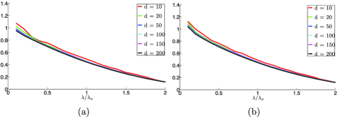
Figure 1: Average number of true discoveries normalized by subspace dimension for values of $\lambda$ in an interval including the heuristic $\lambda_{o}=1/\sqrt{d}$. (a) $\sigma=0.25$. (b) $\sigma=0.5$.

Here, we fix a single subspace in $\mathbb{R}^{n}$ with $n={}$2000. We use a sampling density equal to $\rho=5$ and vary the dimension $d\in\{10,20,50,100,150,200\}$ of the subspace as well as the noise level $\sigma\in\{0.25,0.5\}$. For each data point, we solve (4) for different values of $\lambda$ around the heuristic $\lambda_{o}=1/\sqrt{d}$, namely, $\lambda\in[0.1\lambda_{o},2\lambda_{o}]$. In our experiments, we declare a discovery if an entry in the optimal solution exceeds $10^{-3}$. Figure 1(a) and (b) shows the number of discoveries per subspace dimension (the number of discoveries divided by $d$). One can clearly see that the curves corresponding to various subspace dimensions stack up on top of each other, thereby confirming that a value of $\lambda$ on the order of $1/\sqrt{d}$ yields a fixed fraction of true discoveries. Further inspection also reveals that the fraction of true discoveries is around $50\%$ near $\lambda=\lambda_{o}$, and around $75\%$ near $\lambda=\lambda_{o}/2$. We have observed empirically that increasing $\rho$ typically yields a slight increase in the fraction of true discoveries (unless, of course, $\rho$ is exponentially large in $d$).

2.4.3 The false-true discovery trade off.

We now show empirically that in our model choosing $\lambda$ around $1/\sqrt{d}$ typically yields very few false discoveries as well as many true discoveries; this holds with the proviso that the subspaces are of course not very close to each other.

In this simulation, $22$ subspaces of varying dimensions in $\mathbb{R}^{n}$ with $n={}$2000 have been independently selected uniformly at random; there are $5$, $4$, $3$, $4$, $4$ and $2$ subspaces of respective dimensions $200$, $150$, $100$, $50$, $20$ and $10$. This is a challenging regime since the sum of the subspace dimensions equals 2200 and exceeds the ambient dimension (the clean data matrix $\mathbf{X}$ has full rank). We use a sampling density equal to $\rho=5$ for each subspace and set the noise level to $\sigma=0.3$. To evaluate the performance of the optimization problem (4), we proceed by selecting a subset of columns as follows: for each dimension, we take $100$ cases at random belonging to subspaces of that dimension. Hence, the total number of test cases is $m=600$ so that we only solve $m$ optimization problems (4) out of the total $N$ possible cases. Below, $\bolds{\beta}^{(i)}$ is the solution to (4) and $\bolds{\beta}^{(i)}_{S}$ its restriction to columns with indices in the same subspace. Hence, a nonvanishing entry in $\bolds{\beta}^{(i)}_{S}$ is a true discovery, and likewise, a nonvanishing entry in $\bolds{\beta}^{(i)}_{S^{c}}$ is false. For each data point, we sweep the tuning parameter $\lambda$ in (4) around the heuristic $\lambda_{o}=1/\sqrt{d}$ and work with $\lambda\in[0.05\lambda_{o},2.5\lambda_{o}]$. In our experiments, a discovery is a value obeying $|B_{ij}|>10^{-3}$.

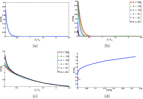
Figure 2: Performance of LASSO for values of $\lambda$ in an interval including the heuristic $\lambda_{o}=1/\sqrt{d}$. (a) Average number of false discoveries normalized by $(n-d)$ (FPR) on all $m$ sampled data points. (b) FPR for different subspace dimensions. Each curve represents the average FPR over those samples originating from subspaces of the same dimension. (c) Average number of true discoveries per dimension for various dimensions (TPR). (d) TPR vs. FPR (ROC curve). The point corresponding to $\lambda=\lambda_{o}$ is marked as a red dot.

In analogy with the signal detection literature, we view the empirical averages of $\|\bolds{\beta}^{(i)}_{S^{c}}\|_{\ell_{0}}/(n-d)$ and $\|\bolds{\beta}^{(i)}_{S}\|_{\ell_{0}}/d$ as False Positive Rate (FPR) and True Positive Rate (TPR). On the one hand, Figure 2(a) and (b) shows that for values around $\lambda=\lambda_{o}$, the FPR is zero (so there are no false discoveries). On the other hand, Figure 2(c) shows that the TPR curves corresponding to different dimensions are very close to each other and resemble those in Figure 2(c) in which all the points belong to the same cluster with no opportunity of making a false discovery. Hence, taking $\lambda$ near $1/\sqrt{d}$ gives a performance close to what can be achieved in a noiseless situation. That is to say, we have no false discovery and a number of true discoveries about $d/2$ if we choose $\lambda=\lambda_{o}$. Figure 2(d) plots TPR versus FPR [a.k.a. the Receiver Operating Characteristic (ROC) curve] and indicates that $\lambda=\lambda_{o}$ (marked by a red dot) is an attractive trade-off as it provides no false discoveries and sufficiently many true discoveries.

2.4.4 A two-step procedure.

Returning to the selection of the regularization parameter, we would like to use $\lambda$ on the order of $1/\sqrt{d}$. However, we do not know $d$ and proceed by substituting an estimate. In the next section, we will see that we are able to quantify theoretically the performance of the following proposal: (1) run a hard constrained version of the LASSO and use an estimate $\hat{d}$ of dimension based on the $\ell_{1}$ norm of the fitted coefficient sequence; (2) impute a value for $\lambda$ constructed from $\hat{d}$. The two-step procedure is explained in Algorithm 2. Again, our exposition is informal here and we refer to Section 3 for precise statements.

Algorithm 2 Two-step procedure with data-driven regularization

  for $i=1,\ldots,N$ do

     1. Solve

$$\bolds{\beta}^{\star}=\arg\min_{\bolds{\beta}\in\mathbb{R}^{N}}\|\bolds{\beta}\|_{\ell_{1}}\qquad\mbox{subject to }\|\mathbf{y}_{i}-\mathbf{Y}\bolds{\bolds{\beta}}\|_{\ell_{2}}\leq\tau\quad\mbox{and}\quad\bolds{\beta}_{i}=0.$$ (6)

     2. Set $\lambda=f(\|\bolds{\beta}^{\star}\|_{\ell_{1}})$.

     3. Solve

$$\hat{\bolds{\beta}}=\arg\min_{\bolds{\beta}\in\mathbb{R}^{N}}\frac{1}{2}\|\mathbf{y}_{i}-\mathbf{Y}\bolds{\beta}\|_{\ell_{2}}^{2}+\lambda\|\bolds{\beta}\|_{\ell_{1}}\qquad\mbox{subject to }\bolds{\beta}_{i}=0.$$

     4. Set $\mathbf{B}_{i}=\hat{\bolds{\beta}}$.

  end for

To understand the rationale behind this, imagine we have noiseless data—that is, $\mathbf{Y}=\mathbf{X}$—and are solving (3), which simply is our first step (6) with the proviso that $\tau=0$. When there are no false discoveries, one can show that the $\ell_{1}$ norm of $\bolds{\beta}^{\star}$ is roughly of size $\sqrt{d}$ as shown in Lemma A.2 from the supplemental article RSCsupp . This suggests using a multiple of $\|\bolds{\beta}^{\star}\|_{\ell_{1}}$ as a proxy for $\sqrt{d}$. To drive this point home, take a look at Figure 3(a) which solves (6) with the same data as in the previous example and $\tau=2\sigma$. The plot reveals that the values of $\|\bolds{\beta}^{\star}\|_{\ell_{1}}$ fluctuate around $\sqrt{d}$. This is shown more clearly in Figure 3(b), which shows that $\|\bolds{\beta}^{\star}\|_{\ell_{1}}$ is concentrated around $\frac{1}{4}\sqrt{d}$ with, as expected, higher volatility at lower values of dimension.

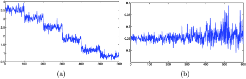
Figure 3: Optimal values of (6) for $600$ samples using $\tau=2\sigma$. The first $100$ values correspond to points originating from subspaces of dimension $d=200$, the next $100$ from those of dimension $d=150$, and so on through $d\in\{100,50,20,10\}$. (a) Value of $\|\bolds{\beta}^{*}\|_{\ell_{1}}$. (b) Value of $\|\bolds{\beta}^{*}\|_{\ell_{1}}/\sqrt{d}$.

Under suitable assumptions, we shall see in Section 3 that with noisy data, there are simple rules for selecting $\tau$ that guarantee, with high probability, that there are no false discoveries. To be concrete, one can take $\tau=2\sigma$ and $f(t)\propto t^{-1}$. Returning to our running example, we have $\|\bolds{\beta}^{\star}\|_{\ell_{1}}\approx\frac{1}{4}\sqrt{d}$. Plugging this into $\lambda=1/\sqrt{d}$ suggests taking $f(t)\approx 0.25t^{-1}$. The plots in Figure 4 demonstrate that this is indeed effective. Experiments in Section 6 indicate that this is a good choice on real data as well.

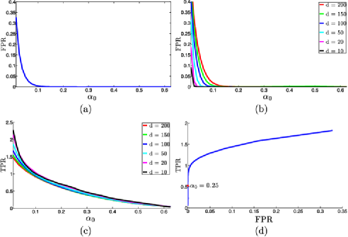
Figure 4: Performance of the two-step procedure using $\tau=2\sigma$ and $f(t)=\alpha_{0}t^{-1}$ for values of $\alpha_{0}$ around the heuristic $\alpha_{0}=0.25$. (a) False positive rate (FPR). (b) FPR for various subspace dimensions. (c) True positive rate (TPR). (d) TPR vs. FPR.

The two-step procedure requires solving two LASSO problems for each data point and is useful when there are subspaces of large dimensions (in the hundreds, say) and some others of low-dimensions (three or four, say). In some applications such as motion segmentation in computer vision, the dimensions of the subspaces are all equal and known in advance tomasi1992shape . In this case, one can forgo the two-step procedure and simply set $\lambda=1/\sqrt{d}$.

3 Theoretical results.

This section presents our main theoretical results concerning the performance of the two-step procedure (Algorithm 2). We defer the proof of these results to the supplemental article RSCsupp . We make two assumptions:

• Affinity condition. We say that a subspace $S_{\ell}$ obeys the affinity condition if

  $$\max_{k\dvtx k\neq\ell}\operatorname{aff}(S_{\ell},S_{k})\leq{\kappa_{0}}/{\log N},$$ (7)

  where $\kappa_{0}$ a fixed numerical constant.

• Sampling condition. We say that subspace $S_{\ell}$ obeys the sampling condition if

  $$\rho_{\ell}\geq\rho^{\star},$$ (8)

  where $\rho^{\star}$ is a fixed numerical constant.

The careful reader might argue that we should require smaller affinity values as the noise level increases. The reason why $\sigma$ does not appear in (7) is that we assumed a bounded noise level. For higher values of $\sigma$, the affinity condition would read as in (7) with a right-hand side equal to

$$\kappa=\frac{\kappa_{0}}{\log N}-\sigma\sqrt{\frac{d_{\ell}}{2n\log N}}.$$

3.1 Main results.

From here on, we use $d(i)$ to refer to the dimension of the subspace the vector $\mathbf{y}_{i}$ originates from. $N(i)$ and $\rho(i)$ are used in a similar fashion for the number and density of points on this subspace.

Theorem 3.1 ((No false discoveries))

Assume that the subspace attached to the $i$th column obeys the affinity and sampling conditions and that the noise level $\sigma$ is bounded as in (2), where $\sigma^{\star}$ is a sufficiently small numerical constant. In Algorithm 2, take $\tau=2\sigma$ and $f(t)$ obeying $f(t)\geq 0.707\sigma t^{-1}$. Then with high probability, there is no false discovery in the $i$th column of $\mathbf{B}$.

Theorem 3.2 ((Many true discoveries))

Consider the same setup as in Theorem 3.1 with $f(\cdot)$ also obeying $f(t)\leq\alpha_{0}t^{-1}$ for some numerical constant $\alpha_{0}$. Then with high probability, there are at least

$$c_{1}\frac{d(i)}{\log\rho(i)}$$ (9)

true discoveries in the $i$th column ($c_{1}$ is a positive numerical constant).

The above results indicate that the first step of the algorithm works correctly in fairly broad conditions. To give an example, assume two subspaces of dimension $d$ overlap in a smaller subspace of dimension $s$ but are orthogonal to each other in the remaining directions (equivalently, the first $s$ principal angles are $0$ and the rest are $\pi/2$). In this case, the affinity between the two subspaces is equal to $\sqrt{s/d}$ and (7) allows $s$ to grow almost linearly in the dimension of the subspaces. Hence, subspaces can have intersections of large dimensions. In contrast, previous work with perfectly noiseless data elhamifar2010clustering would impose to have a first principal angle obeying $|\cos\theta^{(1)}|\leq{1}/{\sqrt{d}}$ so that the subspaces are practically orthogonal to each other. Whereas our result shows that we can have an average of the cosines practically constant, the condition in elhamifar2010clustering asks that the maximum cosine be very small.

In the noiseless case, ourSSC showed that when the sampling condition holds and

$$\max_{k\dvtx k\neq\ell}\operatorname{aff}(S_{\ell},S_{k})\leq\kappa_{0}\frac{\sqrt{\log\rho_{\ell}}}{\log N}$$

(albeit with slightly different values $\kappa_{0}$ and $\rho^{\star}$), then applying the noiseless version (3) of the algorithm also yields no false discoveries. Hence, with the proviso that the noise level is not too large, conditions under which the algorithm is provably correct are essentially the same.

Earlier, we argued that we would like to have, if possible, an algorithm provably working at (1) high values of the affinity parameters and (2) low values of the sampling density as these are the conditions under which the clustering problem is challenging. (Another property on the wish list is the ability to operate properly with high noise or low SNR and this is discussed next.) In this context, since the affinity is at most one, our results state that the affinity can be within a log factor from this maximum possible value. The number of samples needed per subspace is minimal as well. That is, as long as the density of points on each subspace is larger than a constant $\rho>\rho^{\star}$, the algorithm succeeds.

We would like to have a procedure capable of making no false discoveries and many true discoveries at the same time. Now in the noiseless case, whenever there are no false discoveries, the $i$th column contains exactly $d(i)$ true discoveries. Theorem 3.2 states that as long as the noise level $\sigma$ is less than a fixed numerical constant, the number of true discoveries is roughly on the same order as in the noiseless case. In other words, a noise level of this magnitude does not fundamentally affect the performance of the algorithm. This holds even when there is great variation in the dimensions of the subspaces, and is possible because $\lambda$ is appropriately tuned in an adaptive fashion.

The number of true discoveries is shown to scale at least like dimension over the log of the density. This may suggest that the number of true discoveries decreases (albeit very slowly) as the sampling density increases. This behavior is to be expected: when the sampling density becomes exponentially large (in terms of the dimension of the subspace) the number of true discoveries become small since we need fewer columns to synthesize a point. In fact, the $d/\log\rho$ behavior seems to be the correct scaling. Indeed, when the density is low and $\rho$ takes on a small value, (9) asserts that we make on the order of $d$ discoveries, which is tight. Imagine now that we are in the high-density regime and $\rho$ is exponential in $d$. Then as the points gets tightly packed, we expect to have only one discovery in accordance with (9).

Theorem 3.2 establishes that there are many true discoveries. This would not be useful for clustering purposes if there were only a handful of very large true discoveries and all the others of negligible magnitude. The reason is that the similarity matrix $\mathbf{W}$ would then be close to a sparse matrix and we would run the risk of splitting true clusters. Our proofs show that this does not happen although we do not present an argument for lack of space. Rather, we demonstrate this property empirically. On our running example, Figure 5(a) and (b) shows that the histograms of appropriately normalized true discovery values resemble a bell-shaped curve. Note that each true discovery corresponds to a nonzero coefficient which can take on either a positive or negative value.

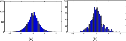
Figure 5: Histograms of the true discovery values from the two step procedure with $\alpha_{0}=0.25$ (multiplied by $\sqrt{d}$). (a) $d=200$. (b) $d=20$.

As stated numerous times, our theoretical analysis only concerns the first step of the algorithm. We now wish to explain how these theoretical results relate to complete guarantees for clustering. First, Theorem 3.1 states that clusters that should be disconnected from each other are, in fact, disconnected so that the algorithm does not group together points from different subspaces. To guarantee perfect clustering, it is then sufficient to show that each restriction of the similarity graph to a subspace is connected. Due to the nature of the random model under study, a subgraph resembles an Erdős–Rèyni graph with the probability of having an edge roughly proportional to the number of true discoveries. As long as there are sufficiently many true discoveries (as shown in Theorem 3.2), such a graph is well connected—in fact, it has very good expansion properties. Proving that each subgraph is indeed connected is a problem we regard as interesting, the main challenge being caused by the dependencies the algorithm generates. Second, a more quantitative characterization of the expansion or connectedness of each subgraph via Cheeger’s constant or the eigenvalue gap may ultimately demonstrate that the algorithm succeeds even in the presence of few false discoveries with small values of $W_{ij}$; please see kannan2009spectral and references therein.

Finally, we would like to comment on the fact that our main results hold when $\lambda$ belongs to a fairly broad range of values. First, when all the subspaces have small dimensions, one can choose the same value of $\lambda$ for all the data points since $1/\sqrt{d}$ is essentially constant. Hence, when we know a priori that we are in such a situation, there may be no need for the two-step procedure. (We would still recommend the conservative two-step procedure because of its superior empirical performance on real data.) Second, the proofs also reveal that if we have knowledge of the dimension of the largest subspace $d_{\max}$, the first theorem holds with a fixed value of $\lambda$ proportional to $\sigma/\sqrt{d_{\max}}$. Third, when the subspaces themselves are drawn at random, the first theorem holds with a fixed value of $\lambda$ proportional to $\sigma(\log N)/\sqrt{n}$. (Both these statements follow by plugging these values of $\lambda$ in the proofs of the supplemental article RSCsupp and we omit the calculations.) We merely mention these variants to give a sense of what our theorems can also give. As explained earlier, we recommend the more conservative two-step procedure with the proxy for $1/\sqrt{d}$. The reason is that using a higher value of $\lambda$ allows for a larger value of $\kappa_{0}$ in (7), which says that the subspaces can be even closer. In other words, we can function in a more challenging regime. To drive this point home, consider the noiseless problem. When the subspaces are close, the equality constrained $\ell_{1}$ problem may yield some false discoveries. However, if we use the LASSO version—even though the data is noiseless—we may end up with no false discoveries while maintaining sufficiently many true discoveries.

4 The bias-corrected Dantzig selector.

One can think of other ways of performing the first step in Algorithm 1 and this section discusses another approach based on a modification of the Dantzig selector, a popular sparse regression technique dantzig . Unlike the two-step procedure, we do not claim any theoretical guarantees for this method and shall only explore its properties on real and simulated data.

Applied directly to our problem, the Dantzig selector takes the form

$$\qquad\min_{\bolds{\beta}\in\mathbb{R}^{N}}\|\bolds{\beta}\|_{\ell_{1}}\qquad\mbox{subject to }\bigl{\|}\mathbf{Y}_{(-i)}^{T}(\mathbf{y}_{i}-\mathbf{Y}\bolds{\bolds{\beta}})\bigr{\|}_{\ell_{\infty}}\leq\lambda\quad\mbox{and}\quad\bolds{\beta}_{i}=0,$$ (10)

where $\mathbf{Y}_{(-i)}$ is $\mathbf{Y}$ with the $i$th column deleted. However, this is hardly suitable since the design matrix $\mathbf{Y}$ is corrupted. Interestingly, recent work MUS , ImprovedMUS has studied the problem of estimating a sparse vector from the standard linear model under uncertainty in the design matrix. The setup in these papers is close to our problem and we propose a modified Dantzig selection procedure inspired but not identical to the methods set forth in MUS , ImprovedMUS .

4.1 The correction.

If we had clean data, we would solve (3); this is (10) with $\mathbf{Y}=\mathbf{X}$ and $\lambda=0$. Let $\bolds{\beta}^{I}$ be the solution to this ideal noiseless problem. Applied to our problem, the main idea in MUS , ImprovedMUS would be to find a formulation that resembles (10) with the property that $\bolds{\beta}^{I}$ is feasible. Since $\mathbf{x}_{i}=\mathbf{X}_{(-i)}{\bolds{\beta}^{I}}_{(-i)}$, observe that we have the following decomposition:

$$\mathbf{Y}_{(-i)}^{T}\bigl{(}\mathbf{y}_{i}-\mathbf{Y}\bolds{\beta}^{I}\bigr{)} = (\mathbf{X}_{(-i)}+\mathbf{Z}_{(-i)})^{T}\bigl{(}\mathbf{z}_{i}-\mathbf{Z}\bolds{\beta}^{I}\bigr{)}$$

$$= \mathbf{X}_{(-i)}^{T}\bigl{(}\mathbf{z}_{i}-\mathbf{Z}\bolds{\beta}^{I}\bigr{)}+\mathbf{Z}_{(-i)}^{T}\mathbf{z}_{i}-\mathbf{Z}_{(-i)}^{T}\mathbf{Z}\bolds{\beta}^{I}.$$

Then the conditional mean is given by

$$\operatorname{\mathbb{E}}\bigl{[}\mathbf{Y}_{(-i)}^{T}\bigl{(}\mathbf{y}_{i}-\mathbf{Y}\bolds{\beta}^{I}\bigr{)}|\mathbf{X}\bigr{]}=-\operatorname{\mathbb{E}}\mathbf{Z}_{(-i)}^{T}\mathbf{Z}_{(-i)}{\bolds{\beta}^{I}}_{(-i)}=-\sigma^{2}{\bolds{\beta}^{I}}_{(-i)}.$$

In other words,

$$\sigma^{2}{\bolds{\beta}^{I}}_{(-i)}+\mathbf{Y}_{(-i)}^{T}\bigl{(}\mathbf{y}_{i}-\mathbf{Y}\bolds{\beta}^{I}\bigr{)}=\bolds{\xi},$$

where $\bolds{\xi}$ has mean zero. In Section 4.2, we compute the variance of the $j$th component $\xi_{j}$, given by

$$\operatorname{\mathbb{E}}\xi_{j}^{2}=\frac{\sigma^{2}}{n}\bigl{(}1+\bigl{\|}\bolds{\beta}^{I}\bigr{\|}_{\ell_{2}}^{2}\bigr{)}+\frac{\sigma^{4}}{n}\bigl{(}1+\bigl{(}\beta^{I}_{j}\bigr{)}^{2}+\bigl{\|}\bolds{\beta}^{I}\bigr{\|}^{2}_{\ell_{2}}\bigr{)}.$$ (11)

Owing to our Gaussian assumptions, $|\xi_{j}|$ shall be smaller than 3 or 4 times this standard deviation, say, with high probability.

Hence, we may want to consider a procedure of the form

$$\min_{\bolds{\beta}\in\mathbb{R}^{N}}\|\bolds{\beta}\|_{\ell_{1}}\qquad\mbox{subject to }\bigl{\|}\mathbf{Y}_{(-i)}^{T}(\mathbf{y}_{i}-\mathbf{Y}\bolds{\bolds{\beta}})+\sigma^{2}\bolds{\beta}_{(-i)}\bigr{\|}_{\ell_{\infty}}\leq\lambda\quad\mbox{and}$$

$$\bolds{\beta}_{i}=0.$$

It follows that if we take $\lambda$ to be a reasonable multiple of (11), then $\bolds{\beta}^{I}$ would obey the constraint in (4.1) with high probability. Hence, we would need to approximate the variance (11). Numerical simulations together with asymptotic calculations presented in the supplemental article RSCsupp give that $\|\bolds{\beta}^{I}\|_{\ell_{2}}\leq 1$ with very high probability. Thus, neglecting the term in $(\beta^{I}_{j})^{2}$,

$$\operatorname{\mathbb{E}}\xi_{j}^{2}\approx\frac{\sigma^{2}}{n}\bigl{(}1+\sigma^{2}\bigr{)}\bigl{(}1+\bigl{\|}\bolds{\beta}^{I}\bigr{\|}_{\ell_{2}}^{2}\bigr{)}\leq 2\frac{\sigma^{2}}{n}\bigl{(}1+\sigma^{2}\bigr{)}.$$

This suggests taking $\lambda$ to be a multiple of $\sqrt{2/n}\sigma\sqrt{1+\sigma^{2}}$. This is interesting because the parameter $\lambda$ does not depend on the dimension of the underlying subspace. We shall refer to (4.1) as the bias-corrected Dantzig selector, which resembles the proposal in MUS , ImprovedMUS for which the constraint is a bit more complicated and of the form $\|\mathbf{Y}_{(-i)}^{T}(\mathbf{y}_{i}-\mathbf{Y}\bolds{\bolds{\beta}})+\mathbf{D}_{(-i)}\bolds{\beta}\|_{\ell_{\infty}}\leq\mu\|\bolds{\beta}\|_{\ell_{1}}+\lambda$.

To get a sense about the validity of this proposal, we test it on our running example by varying $\lambda\in[\lambda_{o},8\lambda_{o}]$ around the heuristic $\lambda_{o}=\sqrt{2/n}\sigma\sqrt{1+\sigma^{2}}$. Figure 6 shows that good results are achieved around factors in the range $[4,6]$.

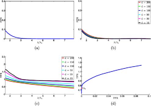
Figure 6: Performance of the bias-corrected Dantzig selector for values of $\lambda$ that are multiples of the heuristic $\lambda_{o}=\sqrt{2/n}\sigma\sqrt{1+\sigma^{2}}$. (a) False positive rate (FPR). (b) FPR for different subspace dimensions. (c) True positive rate (TPR). (d) TPR vs. FPR.

In our synthetic simulations, both the two-step procedure and the corrected Dantzig selector seem to be working well in the sense that they yield many true discoveries while making very few false discoveries, if any. Comparing Figure 6(b) and (c) with those from Section 2 show that the corrected Dantzig selector has more true discoveries for subspaces of small dimensions (they are essentially the same for subspaces of large dimensions); that is, the two-step procedure is more conservative when it comes to subspaces of smaller dimensions. As explained earlier, this is due to our conservative choice of $\lambda$ resulting in a TPR about half of what is obtained in a noiseless setting. Having said this, it is important to keep in mind that in these simulations the planes are drawn at random and as a result, they are sort of far from each other. This is why a less conservative procedure can still achieve a low FPR. When subspaces of smaller dimensions are closer to each other or when the statistical model does not hold exactly as in real data scenarios, a conservative procedure may be more effective. In fact, experiments on real data in Section 6 confirm this and show that for the corrected Dantzig selector, one needs to choose values much larger than $\lambda_{o}$ to yield good results.

4.2 Variance calculation.

By definition,

$$\xi_{j} = \bigl{\langle}\mathbf{x}_{j},\mathbf{z}_{i}-\mathbf{Z}\bolds{\beta}^{I}\bigr{\rangle}+\langle\mathbf{z}_{j},\mathbf{z}_{i}\rangle-\bigl{(}\mathbf{z}_{j}^{T}\mathbf{z}_{j}-\sigma^{2}\bigr{)}\beta^{I}_{j}-\sum_{k\dvtx k\neq i,j}\mathbf{z}_{j}^{T}\mathbf{z}_{k}\beta^{I}_{k}$$

$$:= I_{1}+I_{2}+I_{3}+I_{4}.$$

A simple calculation shows that for $\ell_{1}\neq\ell_{2}$, $\operatorname{Cov}(I_{\ell_{1}},I_{\ell_{2}})=0$ so that

$$\operatorname{\mathbb{E}}\xi_{j}^{2}=\sum_{\ell=1}^{4}\operatorname{Var}(I_{\ell}).$$

We compute

$$\operatorname{Var}(I_{1}) = \frac{\sigma^{2}}{n}\bigl{(}1+\bigl{\|}\bolds{\beta}^{I}\bigr{\|}_{\ell_{2}}^{2}\bigr{)},\qquad\operatorname{Var}(I_{3})=\frac{\sigma^{4}}{n}2\bigl{(}\beta_{j}^{I}\bigr{)}^{2},$$

$$\operatorname{Var}(I_{2}) = \frac{\sigma^{4}}{n},\qquad\operatorname{Var}(I_{4})=\frac{\sigma^{4}}{n}\bigl{[}\bigl{\|}\bolds{\beta}^{I}\bigr{\|}_{\ell_{2}}^{2}-\bigl{(}\beta_{j}^{I}\bigr{)}^{2}\bigr{]}$$

and (11) follows.

5 Comparisons with other works.

We now briefly comment on other approaches to subspace clustering. Since this paper is theoretical in nature, we shall focus on comparing theoretical properties and refer to SSCalg , vidaltutorial for a detailed comparison about empirical performance. Three themes will help in organizing our discussion.

• Tractability. Is the proposed method or algorithm computationally tractable?

• Robustness. Is the algorithm provably robust to noise and other imperfections?

• Efficiency. Is the algorithm correctly operating near the limits we have identified above? In our model, how many points do we need per subspace? How large can the affinity between subspaces be?

One can broadly classify existing subspace clustering techniques into four categories, namely, algebraic, iterative, statistical and spectral clustering-based methods.

Methods inspired from algebraic geometry have been introduced for clustering purposes. In this area, a mathematically intriguing approach is the generalized principal component analysis (GPCA) presented in GPCA . Unfortunately, this algorithm is not tractable in the dimension of the subspaces, meaning that a polynomial-time algorithm does not exist. Another feature is that GPCA is not robust to noise although some heuristics have been developed to address this issue; see, for example, noisyGPCA . As far as the dependence upon key parameters is concerned, GPCA is essentially optimal. An interesting approach to make GPCA robust is based on semidefinite programming gpcaSDP . However, this novel formulation is still intractable in the dimension of the subspaces and it is not clear how the performance of the algorithm depends upon the parameters of interest.

A representative example of an iterative method—the term is taken from the tutorial vidaltutorial —is the $K$-subspace algorithm ksubspaces , a procedure which can be viewed as a generalization of $K$-means. Here, the subspace clustering problem is formulated as a nonconvex optimization problem over the choice of bases for each subspace as well as a set of variables indicating the correct segmentation. A cost function is then iteratively optimized over the basis and the segmentation variables. Each iteration is computationally tractable. However, due to the nonconvex nature of the problem, the convergence of the sequence of iterates is only guaranteed to a local minimum. As a consequence, the dependence upon the key parameters is not well understood. Furthermore, the algorithm can be sensitive to noise and outliers. Other examples of iterative methods may be found in Bradley , agarwal , luvidal , mediankflat .

Statistical methods typically model the subspace clustering problem as a mixture of degenerate Gaussian observations. Two such approaches are mixtures of probabilistic PCA (MPPCA) MPPCA and agglomerative lossy compression (ALC) ALC . MPPCA seeks to compute a maximum-likelihood estimate of the parameters of the mixture model by using an expected–maximization (EM) style algorithm. ALC searches for a segmentation of the data by minimizing the code length necessary (with a code based on Gaussian mixtures) to fit the points up to a given distortion. Once more, due to the nonconvex nature of these formulations, the dependence upon the key parameters and the noise level is not understood.

Many other methods apply spectral clustering to a specially constructed graph Boult , Yan , zhang2012hybrid , goh2007segmenting , SCC , SCCFOCM , arias , aldroubi2012nearness . They share the same difficulties as stated above and vidaltutorial discusses advantages and drawbacks. An approach of this kind is termed Sparse Curvature Clustering (SCC) SCC , SCCFOCM ; please also see arias , ariasclust . This approach is not tractable in the dimension of the subspaces as it requires building a tensor with $N^{(d+2)}$ entries and involves computations with this tensor. Some theoretical guarantees for this algorithm are given in SCCFOCM although its limits of performance and robustness to noise are not fully understood. An approach similar to SSC is called low-rank representation (LRR) LRR . The LRR algorithm is tractable but its robustness to noise and its dependence upon key parameters is not understood. The work in lerman formulates the robust subspace clustering problem as a nonconvex geometric minimization problem over the Grassmanian. Because of the nonconvexity, this formulation may not be tractable. On the positive side, this algorithm is provably robust and can accommodate noise levels up to $\mathcal{O}(1/(Ld^{3/2}))$. However, the density $\rho$ required for favorable properties to hold is an unknown function of the dimensions of the subspaces (e.g., $\rho$ could depend on $d$ in a super polynomial fashion). Also, the bound on the noise level seems to decrease as the dimension $d$ and number of subspaces $L$ increases. In contrast, our theory requires $\rho\geq\rho^{\star}$ where $\rho^{\star}$ is a fixed numerical constant. While this manuscript was under preparation, we learned of highrankMC which establishes robustness to sparse outliers but with a dependence on the key parameters that is super-polynomial in the dimension of the subspaces demanding $\rho\geq C_{0}d^{\log n}$. (Numerical simulations in highrankMC seem to indicate that $\rho$ cannot be a constant.)

We note that the papers MUS , ImprovedMUS , loh2012high also address regression under corrupted covariates. However, there are three key differences between these studies and our work. First, our results show that LASSO without any change is robust to corrupted covariates whereas these works require modifications to either LASSO or the Dantzig selector. Second, the modeling assumptions for the uncorrupted covariates are significantly different. These papers assume that $\mathbf{X}$ has i.i.d. rows and obeys the restricted eigenvalue condition (REC) whereas we have columns sampled from a mixture model so that the design matrices do not have much in common. Last, for clustering and classification purposes, we need to verify that the support of the solution is correct whereas these works establish closeness to an oracle solution in an $\ell_{2}$ sense. In short, our work is far closer to multiple hypothesis testing.

Finally, in the data mining literature subspace clustering is sometimes used to describe a different—although related—problem; see muller2009evaluating , gunnemann2011flexible , keller2012hics .

6 Numerical experiments.

In this section, we perform numerical experiments corroborating our main results and suggesting their applications to temporal segmentation of motion capture data. In this application, we are given sensor measurements at multiple joints of the human body captured at different time instants. The goal is to segment the sensory data so that each cluster corresponds to the same activity. Here, each data point corresponds to a vector whose elements are the sensor measurements of different joints at a fixed time instant.

We use the Carnegie Mellon Motion Capture dataset (available at http://mocap.cs.cmu.edu), which contains 149 subjects performing several activities (data are provided in MCdata ). The motion capture system uses 42 markers per subject. We consider the data from subject $86$ in the dataset, consisting of $15$ different trials, where each trial comprises multiple activities. We use trials $2$ and $5$, which feature more activities ($8$ activities for trial $2$ and $7$ activities for trial $5$) and are, therefore, harder examples relative to the other trials. Figure 7 shows a few snapshots of each activity (walking, squatting, punching, standing, running, jumping, arms-up and drinking) from trial $2$. The right plot in Figure 7 shows the singular values of three of the activities in this trial. Notice that all the curves have a low-dimensional knee, showing that the data from each activity lie in a low-dimensional subspace of the ambient space ($n=42$ for all the motion capture data).

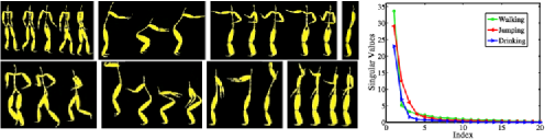
Figure 7: Left: eight activities performed by subject $86$ in the CMU motion capture dataset: walking, squatting, punching, standing, running, jumping, arms-up and drinking. Right: singular values of the data from three activities (walking, jumping, drinking) show that the data from each activity lie approximately in a low-dimensional subspace.

We compare three different algorithms: a baseline algorithm, the two-step procedure and the bias-corrected Dantzig selector. We evaluate these algorithms based on the clustering error. That is, we assume knowledge of the number of subspaces and apply spectral clustering to the similarity matrix built by the algorithm. After the spectral clustering step, the clustering error is simply the ratio of misclassified points to the total number of points. We report our results on half of the examples—downsampling the video by a factor $2$ keeping every other frame—as to make the problem more challenging. (As a side note, it is always desirable to have methods that work well on a smaller number of examples as one can use split-sample strategies for tuning purposes.)

As a baseline for comparison, we apply spectral clustering to a standard similarity graph built by connecting each data point to its $K$-nearest neighbors. For pairs of data points, $\mathbf{y}_{i}$ and $\mathbf{y}_{j}$, that are connected in the $K$-nearest neighbor graph, we define the similarities between them by $W_{ij}=\exp(-\|\mathbf{y}_{i}-\mathbf{y}_{j}\|_{2}^{2}/t)$, where $t>0$ is a tuning parameter (a.k.a. temperature). For pairs of data points, $\mathbf{y}_{i}$ and $\mathbf{y}_{j}$, that are not connected in the $K$-nearest neighbor graph, we set $W_{ij}=0$. Thus, pairs of neighboring data points that have small Euclidean distances from each other are considered to be more similar, since they have high similarity $W_{ij}$. We then apply spectral clustering to the similarity graph and measure the clustering error. For each value of $K$, we record the minimum clustering error over different choices of the temperature parameter $t>0$ as shown in Figure 8(a) and (b). The minimum clustering error for trials $2$ and $5$ are $17.06\%$ and $12.47\%$.

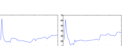
Figure 8: Minimum clustering error ($\%$) for each $K$ in the baseline algorithm.

For solving the LASSO problems in the two-step procedure, we developed a computational routine made publicly available MSweb based on TFOCS TFOCS solving the optimization problems in parallel. For the corrected Dantzig selector, we use a homotopy solver in the spirit of homotopy .

For both the two-step procedure and the bias-corrected Dantzig selector, we normalize the data points as a preprocessing step. We work with a noise $\sigma$ in the interval $[0.001,0.045]$, and use $f(t)=\alpha/t$ with values of $\alpha$ around $1/4$ (this is equivalent to varying $\lambda$ around $1/\lambda_{o}=4\|\bolds{\beta}^{\star}\|_{\ell_{1}}$) in the two-step procedure. For the bias-corrected Dantzig selector, we vary $\lambda$ around $\lambda_{o}=\sqrt{2/n}\sigma\sqrt{1+\sigma^{2}}$. After building the similarity graph from the sparse regression output, we apply spectral clustering as explained earlier. Figures 9(a) and (b), 10(a) and (b) show the clustering error (on trial $5$) and the red point indicates the location where the minimum clustering error is reached. Figure 9(a) and (b) shows that for the two-step procedure the value of the clustering error is not overly sensitive to the choice of $\sigma$—especially around $\lambda=\lambda_{o}$. Notice that the clustering error for the robust versions of SSC are significantly lower than the baseline algorithm for a wide range of parameter values. The reason the baseline algorithm performs poorly in this case is that there are many points that are in small Euclidean distances from each other, but belong to different subspaces.

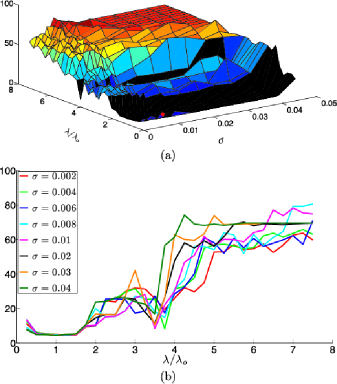
Figure 9: Clustering error (%) for different values of $\lambda$ and $\sigma$ on trial $5$ using the two-step procedure (a) 3D plot (minimum clustering error appears in red). (b) 2D cross sections.

Finally a summary of the clustering errors of these algorithms on the two trials are reported in Table 1. Robust versions of SSC outperform the baseline algorithm. This shows that the multiple subspace model is better for clustering purposes. The two-step procedure seems to work slightly better than the corrected Dantzig selector for these two examples. Table 2 reports the optimal parameters that achieve the minimum clustering error for each algorithm. The table indicates that on real data, choosing $\lambda$ close to $\lambda_{o}$ also works very well. Also, one can see that in comparison with the synthetic simulations of Section 4, a more conservative choice of the regularization parameter $\lambda$ is needed for the corrected Dantzig selector as $\lambda$ needs to be chosen much higher than $\lambda_{o}$ to achieve the best results. This may be attributed to the fact that the subspaces in this example are very close to each other and are not drawn at random as was the case with our synthetic data. To get a sense of the affinity values, we fit a subspace of dimension $d_{\ell}$ to the $N_{\ell}$ data points from the $\ell$th group, where $d_{\ell}$ is chosen as the smallest nonnegative integer such that the partial sum of the $d_{\ell}$ top singular values is at least 90% of the total sum. Figure 11 shows that the affinities are higher than $0.75$ for both trials.

7 Discussion and open problems.

In this paper, we have developed a tractable algorithm that can provably cluster data points in a fairly challenging regime in which subspaces can overlap along many dimensions and in which the number of points per subspace is rather limited.

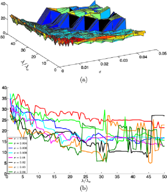
Figure 10: Clustering error (%) for different values of $\lambda$ and $\sigma$ on trial $5$ using the corrected Dantzig selector. (a) 3D plot (minimum clustering error appears in red). (b) 2D cross sections.

Table 1: Minimum clustering error

	Baseline algorithm	Two-step procedure	Corrected Dantzig selector
Trial 2	17.06%	3.54%	9.53%
Trial 5	12.47%	4.35%	4.92%

Our results about the performance of the robust SSC algorithm are expressed in terms of interpretable parameters. This is not a trivial achievement: one of the challenges of the theory for subspace clustering is precisely that performance depends on many different aspects of the problem such as the dimension of the ambient space, the number of subspaces, their dimensions, their relative orientations, the distribution of points around each subspace, the noise level and so on. Nevertheless, these results only offer a starting point as our work leaves open lots of questions, and at the same time, suggests topics for future research. Before presenting the proofs, we would like to close by listing a few questions colleagues may find of interest.

• We have shown that while having the affinities and sampling densities near what is information theoretically possible, robust versions of SSC that can accommodate noise levels $\sigma$ of order one exist. It would be interesting to establish fundamental limits relating the key parameters to the maximum allowable noise level. What is the maximum allowable noise level for any algorithm regardless of tractability?

• It would be interesting to extend the results of this paper to a deterministic model where both the orientation of the subspaces and the noiseless samples are nonrandom. We leave this to a future publication.

  Table 2: Optimal parameters

  	Baseline algorithm	Two-step procedure	Corrected Dantzig selector
  Trial 2	$K=9$, $t=0.0769$	$\sigma=0.03$, $\lambda=1.25\lambda_{o}$	$\sigma=0.004$, $\lambda=41.5\lambda_{o}$
  Trial 5	$K=6$, $t=0.0455$	$\sigma=0.01$, $\lambda=\lambda_{o}$	$\sigma=0.03$, $\lambda=45.5\lambda_{o}$

  

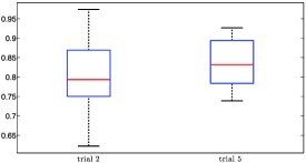
  Figure 11: Box plot of the affinities between subspaces for trials $2$ and $5$.

• Our work in this paper concerns the construction of the similarity matrix and the correctness of sparse regression techniques. The full algorithm then applies clustering techniques to clean up errors introduced in the first step. It would be interesting to develop theoretical guarantees for this step as well. A potential approach is the interesting formulation developed in nina .

• We proposed a two-step procedure for robust subspace clustering. The first step is used to estimate the required regularization parameter for a LASSO problem. This is reminiscent of estimating noise in sparse regularization and covariance estimation. It would be interesting to design a joint optimization scheme to simultaneous optimize the regularization parameter and the regression coefficients. In recent years, there has been much progress on this issue in the sparse regression literature; see belloni2011square , giraud2012high , sun2012scaled , st2010l1 , dalalyan2012fused and references therein. It is an open research direction to see whether any of these approaches can be applied to automatically learn the regularization parameter when both the response vector and covariates are corrupted and, in particular, for the purpose of robust subspace clustering.

• A natural direction is the development of clustering techniques that can provably operate with missing and/or sparsely corrupted entries (the work ourSSC only deals with grossly corrupted columns). The work in highrankMC provides one possible approach but requires a very high sampling density as we already mentioned. The paper SSCalg develops another heuristic approach without any theoretical justification.

• Our formulation uses a data-driven modeling approach by regressing each data point against all others. As noted by Bittorf et al. bittorf2012factoring , this type of approach appears in a number of other factorization problems. In particular, arora2012computing and recent variations arora2012computing , bittorf2012factoring use a convex formulation very similar to SSC for the purpose of nonnegative matrix factorizations. Exploring the connection between these factorization problems is an interesting research direction.

• One of the advantages of the suggested scheme is that it is highly parallelizable. When the algorithm is run sequentially, it would be interesting to see whether one can reuse computations to solve all the $\ell_{1}$-minimization problems more effectively.

References

- (1) {bincollection}[auto:STB—2014/02/12—14:17:21] \bauthor\bsnmAgarwal, \bfnmP. K.\binitsP. K. and \bauthor\bsnmMustafa, \bfnmN. H.\binitsN. H. (\byear2004). \btitle-means projective clustering. In \bbooktitleProceedings of the Twenty-third ACM SIGMOD-SIGACT-SIGART Symposium on Principles of Database Systems \bpages155–165. \bptokimsref\endbibitem
- (2) {barticle}[auto:STB—2014/02/12—14:17:21] \bauthor\bsnmAldroubi, \bfnmA.\binitsA. and \bauthor\bsnmSekmen, \bfnmA.\binitsA. (\byear2012). \btitleNearness to local subspace algorithm for subspace and motion segmentation. \bjournalSignal Process. Lett., IEEE \bvolume19 \bpages704–707. \bptokimsref\endbibitem
- (3) {barticle}[mr] \bauthor\bsnmArias-Castro, \bfnmEry\binitsE. (\byear2011). \btitleClustering based on pairwise distances when the data is of mixed dimensions. \bjournalIEEE Trans. Inform. Theory \bvolume57 \bpages1692–1706. \biddoi=10.1109/TIT.2011.2104630, issn=0018-9448, mr=2815843 \bptokimsref\endbibitem
- (4) {barticle}[mr] \bauthor\bsnmArias-Castro, \bfnmEry\binitsE., \bauthor\bsnmChen, \bfnmGuangliang\binitsG. and \bauthor\bsnmLerman, \bfnmGilad\binitsG. (\byear2011). \btitleSpectral clustering based on local linear approximations. \bjournalElectron. J. Stat. \bvolume5 \bpages1537–1587. \biddoi=10.1214/11-EJS651, issn=1935-7524, mr=2861697 \bptokimsref\endbibitem
- (5) {bincollection}[mr] \bauthor\bsnmArora, \bfnmSanjeev\binitsS., \bauthor\bsnmGe, \bfnmRong\binitsR., \bauthor\bsnmKannan, \bfnmRavi\binitsR. and \bauthor\bsnmMoitra, \bfnmAnkur\binitsA. (\byear2012). \btitleComputing a nonnegative matrix factorization–provably. In \bbooktitleSTOC’12—Proceedings of the 2012 ACM Symposium on Theory of Computing \bpages145–161. \bpublisherACM, \blocationNew York. \biddoi=10.1145/2213977.2213994, mr=2961503 \bptokimsref\endbibitem
- (6) {barticle}[mr] \bauthor\bsnmBako, \bfnmLaurent\binitsL. (\byear2011). \btitleIdentification of switched linear systems via sparse optimization. \bjournalAutomatica J. IFAC \bvolume47 \bpages668–677. \biddoi=10.1016/j.automatica.2011.01.036, issn=0005-1098, mr=2878328 \bptokimsref\endbibitem
- (7) {binproceedings}[mr] \bauthor\bsnmBalcan, \bfnmMaria-Florina\binitsM.-F., \bauthor\bsnmBlum, \bfnmAvrim\binitsA. and \bauthor\bsnmGupta, \bfnmAnupam\binitsA. (\byear2009). \btitleApproximate clustering without the approximation. In \bbooktitleProceedings of the Twentieth Annual ACM–SIAM Symposium on Discrete Algorithms \bpages1068–1077. \bpublisherSIAM, \blocationPhiladelphia, PA. \bidmr=2807549 \bptokimsref\endbibitem
- (8) {barticle}[mr] \bauthor\bsnmBayati, \bfnmMohsen\binitsM. and \bauthor\bsnmMontanari, \bfnmAndrea\binitsA. (\byear2011). \btitleThe dynamics of message passing on dense graphs, with applications to compressed sensing. \bjournalIEEE Trans. Inform. Theory \bvolume57 \bpages764–785. \biddoi=10.1109/TIT.2010.2094817, issn=0018-9448, mr=2810285 \bptokimsref\endbibitem
- (9) {barticle}[mr] \bauthor\bsnmBayati, \bfnmMohsen\binitsM. and \bauthor\bsnmMontanari, \bfnmAndrea\binitsA. (\byear2012). \btitleThe LASSO risk for Gaussian matrices. \bjournalIEEE Trans. Inform. Theory \bvolume58 \bpages1997–2017. \biddoi=10.1109/TIT.2011.2174612, issn=0018-9448, mr=2951312 \bptokimsref\endbibitem
- (10) {barticle}[mr] \bauthor\bsnmBecker, \bfnmStephen R.\binitsS. R., \bauthor\bsnmCandès, \bfnmEmmanuel J.\binitsE. J. and \bauthor\bsnmGrant, \bfnmMichael C.\binitsM. C. (\byear2011). \btitleTemplates for convex cone problems with applications to sparse signal recovery. \bjournalMath. Program. Comput. \bvolume3 \bpages165–218. \biddoi=10.1007/s12532-011-0029-5, issn=1867-2949, mr=2833262 \bptokimsref\endbibitem
- (11) {barticle}[mr] \bauthor\bsnmBelloni, \bfnmA.\binitsA., \bauthor\bsnmChernozhukov, \bfnmV.\binitsV. and \bauthor\bsnmWang, \bfnmL.\binitsL. (\byear2011). \btitleSquare-root lasso: Pivotal recovery of sparse signals via conic programming. \bjournalBiometrika \bvolume98 \bpages791–806. \biddoi=10.1093/biomet/asr043, issn=0006-3444, mr=2860324 \bptokimsref\endbibitem
- (12) {bmisc}[auto:STB—2014/02/12—14:17:21] \bauthor\bsnmBittorf, \bfnmV.\binitsV., \bauthor\bsnmRecht, \bfnmB.\binitsB., \bauthor\bsnmRe, \bfnmC.\binitsC. and \bauthor\bsnmTropp, \bfnmJ. A.\binitsJ. A. (\byear2012). \bhowpublishedFactoring nonnegative matrices with linear programs. In Proceedings of Natural Information Processing Systems Foundation NIPS. \bptokimsref\endbibitem
- (13) {bincollection}[auto:STB—2014/02/12—14:17:21] \bauthor\bsnmBoult, \bfnmT. E.\binitsT. E. and \bauthor\bsnmGottesfeld Brown, \bfnmL.\binitsL. (\byear1991). \btitleFactorization-based segmentation of motions. In \bbooktitleProceedings of the IEEE Workshop on Visual Motion \bpages179–186. \bptokimsref\endbibitem
- (14) {barticle}[mr] \bauthor\bsnmBradley, \bfnmP. S.\binitsP. S. and \bauthor\bsnmMangasarian, \bfnmO. L.\binitsO. L. (\byear2000). \btitle-plane clustering. \bjournalJ. Global Optim. \bvolume16 \bpages23–32. \biddoi=10.1023/A:1008324625522, issn=0925-5001, mr=1770524 \bptokimsref\endbibitem
- (15) {barticle}[mr] \bauthor\bsnmCandès, \bfnmEmmanuel\binitsE. and \bauthor\bsnmTao, \bfnmTerence\binitsT. (\byear2007). \btitleThe Dantzig selector: Statistical estimation when is much larger than . \bjournalAnn. Statist. \bvolume35 \bpages2313–2351. \biddoi=10.1214/009053606000001523, issn=0090-5364, mr=2382644 \bptokimsref\endbibitem
- (16) {barticle}[mr] \bauthor\bsnmChen, \bfnmGuangliang\binitsG. and \bauthor\bsnmLerman, \bfnmGilad\binitsG. (\byear2009). \btitleFoundations of a multi-way spectral clustering framework for hybrid linear modeling. \bjournalFound. Comput. Math. \bvolume9 \bpages517–558. \biddoi=10.1007/s10208-009-9043-7, issn=1615-3375, mr=2534403 \bptokimsref\endbibitem
- (17) {barticle}[auto:STB—2014/02/12—14:17:21] \bauthor\bsnmChen, \bfnmG.\binitsG. and \bauthor\bsnmLerman, \bfnmG.\binitsG. (\byear2009). \btitleSpectral curvature clustering (SCC). \bjournalInt. J. Comput. Vis. \bvolume81 \bpages317–330. \bptokimsref\endbibitem
- (18) {barticle}[auto:STB—2014/02/12—14:17:21] \bauthor\bsnmChen, \bfnmY.\binitsY., \bauthor\bsnmNasrabadi, \bfnmN. M.\binitsN. M. and \bauthor\bsnmTran, \bfnmT. D.\binitsT. D. (\byear2011). \btitleHyperspectral image classification using dictionary-based sparse representation. \bjournalIEEE Trans. Geosci. Remote Sens. \bvolume99 \bpages1–13. \bptokimsref\endbibitem
- (19) {bincollection}[auto:STB—2014/02/12—14:17:21] \bauthor\bsnmDalalyan, \bfnmA.\binitsA. and \bauthor\bsnmChen, \bfnmY.\binitsY. (\byear2012). \btitleFused sparsity and robust estimation for linear models with unknown variance. In \bbooktitleAdvances in Neural Information Processing Systems \bvolume25 \bpages1268–1276. \bptokimsref\endbibitem
- (20) {bincollection}[auto:STB—2014/02/12—14:17:21] \bauthor\bsnmElhamifar, \bfnmE.\binitsE. and \bauthor\bsnmVidal, \bfnmR.\binitsR. (\byear2009). \btitleSparse subspace clustering. In \bbooktitleIEEE Conference on Computer Vision and Pattern Recognition, CVPR \bpages2790–2797. \bptokimsref\endbibitem
- (21) {bincollection}[auto:STB—2014/02/12—14:17:21] \bauthor\bsnmElhamifar, \bfnmE.\binitsE. and \bauthor\bsnmVidal, \bfnmR.\binitsR. (\byear2010). \btitleClustering disjoint subspaces via sparse representation. In \bbooktitleIEEE International Conference on Acoustics Speech and Signal Processing, ICASSP \bpages1926–1929. \bpublisherIEEE Press, \blocationNew York. \bptokimsref\endbibitem
- (22) {barticle}[auto] \bauthor\bsnmElhamifar, \bfnmEhsan\binitsE. and \bauthor\bsnmVidal, \bfnmRené\binitsR. (\byear2013). \btitleSparse subspace clustering: Algorithms, theory, and applications. \bjournalIEEE Trans. Pattern Anal. Mach. Intell. \bvolume35 \bpages2765–2781. \bptokimsref\endbibitem
- (23) {bmisc}[auto:STB—2014/02/12—14:17:21] \bauthor\bsnmEriksson, \bfnmB.\binitsB., \bauthor\bsnmBalzano, \bfnmL.\binitsL. and \bauthor\bsnmNowak, \bfnmR.\binitsR. (\byear2011). \bhowpublishedHigh-rank matrix completion and subspace clustering with missing data. Preprint. Available at \arxivurlarXiv:1112.5629. \bptokimsref\endbibitem
- (24) {barticle}[mr] \bauthor\bsnmGiraud, \bfnmChristophe\binitsC., \bauthor\bsnmHuet, \bfnmSylvie\binitsS. and \bauthor\bsnmVerzelen, \bfnmNicolas\binitsN. (\byear2012). \btitleHigh-dimensional regression with unknown variance. \bjournalStatist. Sci. \bvolume27 \bpages500–518. \biddoi=10.1214/12-STS398, issn=0883-4237, mr=3025131 \bptokimsref\endbibitem
- (25) {bincollection}[auto:STB—2014/02/12—14:17:21] \bauthor\bsnmGoh, \bfnmA.\binitsA. and \bauthor\bsnmVidal, \bfnmR.\binitsR. (\byear2007). \btitleSegmenting motions of different types by unsupervised manifold clustering. In \bbooktitleIEEE International Conference on Computer Vision and Pattern Recognition, CVPR \bpages1–6. \bpublisherIEEE Press, \blocationNew York. \bptokimsref\endbibitem
- (26) {bincollection}[auto:STB—2014/02/12—14:17:21] \bauthor\bsnmGunnemann, \bfnmS.\binitsS., \bauthor\bsnmMuller, \bfnmE.\binitsE., \bauthor\bsnmRaubach, \bfnmS.\binitsS. and \bauthor\bsnmSeidl, \bfnmT.\binitsT. (\byear2011). \btitleFlexible fault tolerant subspace clustering for data with missing values. In \bbooktitleIEEE International Conference on Data Mining, ICDM \bpages231–240. \bptokimsref\endbibitem
- (27) {barticle}[mr] \bauthor\bsnmKannan, \bfnmRavindran\binitsR. and \bauthor\bsnmVempala, \bfnmSantosh\binitsS. (\byear2008). \btitleSpectral algorithms. \bjournalFound. Trends Theor. Comput. Sci. \bvolume4 \bpages157–288 (2009). \biddoi=10.1561/0400000025, issn=1551-305X, mr=2558901 \bptnotecheck year \bptokimsref\endbibitem
- (28) {bincollection}[auto:STB—2014/02/12—14:17:21] \bauthor\bsnmKeller, \bfnmF.\binitsF., \bauthor\bsnmMuller, \bfnmE.\binitsE. and \bauthor\bsnmBohm, \bfnmK.\binitsK. (\byear2012). \btitleHICS: High contrast subspaces for density-based outlier ranking. In \bbooktitleIEEE International Conference on Data Engineering, ICDE \bpages1037–1048. \bptokimsref\endbibitem
- (29) {bincollection}[auto:STB—2014/02/12—14:17:21] \bauthor\bsnmKotropoulos, \bfnmY. P. C.\binitsY. P. C. and \bauthor\bsnmArce, \bfnmG. R.\binitsG. R. (\byear2011). \btitle-graph based music structure analysis. In \bbooktitleInternational Society for Music Information Retrieval Conference, ISMIR. \bptokimsref\endbibitem
- (30) {barticle}[mr] \bauthor\bsnmLerman, \bfnmGilad\binitsG. and \bauthor\bsnmZhang, \bfnmTeng\binitsT. (\byear2011). \btitleRobust recovery of multiple subspaces by geometric minimization. \bjournalAnn. Statist. \bvolume39 \bpages2686–2715. \biddoi=10.1214/11-AOS914, issn=0090-5364, mr=2906883 \bptokimsref\endbibitem
- (31) {barticle}[auto:STB—2014/02/12—14:17:21] \bauthor\bsnmLiu, \bfnmG.\binitsG., \bauthor\bsnmLin, \bfnmZ.\binitsZ., \bauthor\bsnmYan, \bfnmS.\binitsS., \bauthor\bsnmSun, \bfnmJ.\binitsJ., \bauthor\bsnmYu, \bfnmY.\binitsY. and \bauthor\bsnmMa, \bfnmY.\binitsY. (\byear2013). \btitleRobust recovery of subspace structures by low-rank representation. \bjournalIEEE Trans. Pattern Anal. Mach. Intell. \bvolume35 \bpages171–184. \bptokimsref\endbibitem
- (32) {barticle}[mr] \bauthor\bsnmLoh, \bfnmPo-Ling\binitsP.-L. and \bauthor\bsnmWainwright, \bfnmMartin J.\binitsM. J. (\byear2012). \btitleHigh-dimensional regression with noisy and missing data: Provable guarantees with nonconvexity. \bjournalAnn. Statist. \bvolume40 \bpages1637–1664. \biddoi=10.1214/12-AOS1018, issn=0090-5364, mr=3015038 \bptokimsref\endbibitem
- (33) {bincollection}[auto:STB—2014/02/12—14:17:21] \bauthor\bsnmLu, \bfnmL.\binitsL. and \bauthor\bsnmVidal, \bfnmR.\binitsR. (\byear2006). \btitleCombined central and subspace clustering for computer vision applications. In \bbooktitleProceedings of the 23rd International Conference on Machine Learning \bpages593–600. \bpublisherACM, \blocationNew York. \bptokimsref\endbibitem
- (34) {barticle}[auto:STB—2014/02/12—14:17:21] \bauthor\bsnmMa, \bfnmY.\binitsY., \bauthor\bsnmDerksen, \bfnmH.\binitsH., \bauthor\bsnmHong, \bfnmW.\binitsW. and \bauthor\bsnmWright, \bfnmJ.\binitsJ. (\byear2007). \btitleSegmentation of multivariate mixed data via lossy data coding and compression. \bjournalIEEE Trans. Pattern Anal. Mach. Intell. \bvolume29 \bpages1546–1562. \bptokimsref\endbibitem
- (35) {bincollection}[auto:STB—2014/02/12—14:17:21] \bauthor\bsnmMa, \bfnmY.\binitsY. and \bauthor\bsnmVidal, \bfnmR.\binitsR. (\byear2005). \btitleIdentification of deterministic switched arx systems via identification of algebraic varieties. In \bbooktitleHybrid Systems: Computation and Control \bpages449–465. \bptokimsref\endbibitem
- (36) {barticle}[mr] \bauthor\bsnmMa, \bfnmYi\binitsY., \bauthor\bsnmYang, \bfnmAllen Y.\binitsA. Y., \bauthor\bsnmDerksen, \bfnmHarm\binitsH. and \bauthor\bsnmFossum, \bfnmRobert\binitsR. (\byear2008). \btitleEstimation of subspace arrangements with applications in modeling and segmenting mixed data. \bjournalSIAM Rev. \bvolume50 \bpages413–458. \biddoi=10.1137/060655523, issn=0036-1445, mr=2429444 \bptokimsref\endbibitem
- (37) {barticle}[mr] \bauthor\bsnmMcWilliams, \bfnmBrian\binitsB. and \bauthor\bsnmMontana, \bfnmGiovanni\binitsG. (\byear2014). \btitleSubspace clustering of high-dimensional data: A predictive approach. \bjournalData Min. Knowl. Discov. \bvolume28 \bpages736–772. \biddoi=10.1007/s10618-013-0317-y, issn=1384-5810, mr=3165525 \bptnotecheck year \bptokimsref\endbibitem
- (38) {barticle}[mr] \bauthor\bsnmMeinshausen, \bfnmNicolai\binitsN. and \bauthor\bsnmBühlmann, \bfnmPeter\binitsP. (\byear2006). \btitleHigh-dimensional graphs and variable selection with the lasso. \bjournalAnn. Statist. \bvolume34 \bpages1436–1462. \biddoi=10.1214/009053606000000281, issn=0090-5364, mr=2278363 \bptokimsref\endbibitem
- (39) {barticle}[auto:STB—2014/02/12—14:17:21] \bauthor\bsnmMüller, \bfnmE.\binitsE., \bauthor\bsnmGunnemann, \bfnmS.\binitsS., \bauthor\bsnmAssent, \bfnmI.\binitsI. and \bauthor\bsnmSeidl, \bfnmT.\binitsT. (\byear2009). \btitleEvaluating clustering in subspace projections of high dimensional data. \bjournalProc. VLDB Endow. \bvolume2 \bpages1270–1281. \bptokimsref\endbibitem
- (40) {barticle}[auto:STB—2014/02/12—14:17:21] \bauthor\bsnmNg, \bfnmA. Y.\binitsA. Y., \bauthor\bsnmJordan, \bfnmM. I.\binitsM. I. and \bauthor\bsnmWeiss, \bfnmY.\binitsY. (\byear2002). \btitleOn spectral clustering: Analysis and an algorithm. \bjournalAdv. Neural Inf. Process. Syst. \bvolume2 \bpages849–856. \bptokimsref\endbibitem
- (41) {bincollection}[auto:STB—2014/02/12—14:17:21] \bauthor\bsnmOzay, \bfnmN.\binitsN., \bauthor\bsnmSznaier, \bfnmM.\binitsM. and \bauthor\bsnmLagoa, \bfnmC.\binitsC. (\byear2010). \btitleModel (in) validation of switched arx systems with unknown switches and its application to activity monitoring. In \bbooktitleIEEE Conference on Decision and Control, CDC \bpages7624–7630. \bptokimsref\endbibitem
- (42) {bincollection}[auto:STB—2014/02/12—14:17:21] \bauthor\bsnmOzay, \bfnmN.\binitsN., \bauthor\bsnmSznaier, \bfnmM.\binitsM., \bauthor\bsnmLagoa, \bfnmC.\binitsC. and \bauthor\bsnmCamps, \bfnmO.\binitsO. (\byear2010). \btitleGPCA with denoising: A moments-based convex approach. In \bbooktitleIEEE Conference on Computer Vision and Pattern Recognition, CVPR \bpages3209–3216. \bpublisherIEEE Press, \blocationNew York. \bptokimsref\endbibitem
- (43) {barticle}[auto:STB—2014/02/12—14:17:21] \bauthor\bsnmParsons, \bfnmL.\binitsL., \bauthor\bsnmHaque, \bfnmE.\binitsE. and \bauthor\bsnmLiu, \bfnmH.\binitsH. (\byear2004). \btitleSubspace clustering for high dimensional data: A review. \bjournalACM SIGKDD Explor. Newsl. \bvolume6 \bpages90–105. \bptokimsref\endbibitem
- (44) {binproceedings}[auto:STB—2014/02/12—14:17:21] \bauthor\bsnmRosenbaum, \bfnmM.\binitsM. and \bauthor\bsnmTsybakov, \bfnmA. B.\binitsA. B. (\byear2013). \btitleImproved matrix uncertainty selector. In \bbooktitleFrom Probability to Statistics and Back: High-Dimensional Models and Processes—A Festschrift in Honor of Jon A. Wellner \bpages276–290. \bpublisherIMS, \blocationBeachwood, OH. \bptokimsref\endbibitem
- (45) {barticle}[mr] \bauthor\bsnmRosenbaum, \bfnmMathieu\binitsM. and \bauthor\bsnmTsybakov, \bfnmAlexandre B.\binitsA. B. (\byear2010). \btitleSparse recovery under matrix uncertainty. \bjournalAnn. Statist. \bvolume38 \bpages2620–2651. \biddoi=10.1214/10-AOS793, issn=0090-5364, mr=2722451 \bptokimsref\endbibitem
- (46) {barticle}[mr] \bauthor\bsnmSoltanolkotabi, \bfnmMahdi\binitsM. and \bauthor\bsnmCandés, \bfnmEmmanuel J.\binitsE. J. (\byear2012). \btitleA geometric analysis of subspace clustering with outliers. \bjournalAnn. Statist. \bvolume40 \bpages2195–2238. \biddoi=10.1214/12-AOS1034, issn=0090-5364, mr=3059081 \bptokimsref\endbibitem
- (47) {bmisc}[auto:STB—2014/02/12—14:17:21] \bauthor\bsnmSoltanolkotabi, \bfnmM.\binitsM., \bauthor\bsnmElhamifar, \bfnmE.\binitsE. and \bauthor\bsnmCandès, \bfnmE. J.\binitsE. J. (\byear2014). \bhowpublishedSupplement to “Robust subspace clustering.” DOI:\doiurl10.1214/13-AOS1199SUPP. \bptokimsref\endbibitem
- (48) {barticle}[mr] \bauthor\bsnmStädler, \bfnmNicolas\binitsN., \bauthor\bsnmBühlmann, \bfnmPeter\binitsP. and \bauthor\bparticlevan de \bsnmGeer, \bfnmSara\binitsS. (\byear2010). \btitle-penalization for mixture regression models. \bjournalTEST \bvolume19 \bpages209–256. \biddoi=10.1007/s11749-010-0197-z, issn=1133-0686, mr=2677722 \bptnotecheck related \bptokimsref\endbibitem
- (49) {barticle}[mr] \bauthor\bsnmSun, \bfnmTingni\binitsT. and \bauthor\bsnmZhang, \bfnmCun-Hui\binitsC.-H. (\byear2012). \btitleScaled sparse linear regression. \bjournalBiometrika \bvolume99 \bpages879–898. \biddoi=10.1093/biomet/ass043, issn=0006-3444, mr=2999166 \bptokimsref\endbibitem
- (50) {barticle}[mr] \bauthor\bsnmTipping, \bfnmMichael E.\binitsM. E. and \bauthor\bsnmBishop, \bfnmChristopher M.\binitsC. M. (\byear1999). \btitleProbabilistic principal component analysis. \bjournalJ. R. Stat. Soc. Ser. B Stat. Methodol. \bvolume61 \bpages611–622. \biddoi=10.1111/1467-9868.00196, issn=1369-7412, mr=1707864 \bptokimsref\endbibitem
- (51) {barticle}[auto:STB—2014/02/12—14:17:21] \bauthor\bsnmTomasi, \bfnmC.\binitsC. and \bauthor\bsnmKanade, \bfnmT.\binitsT. (\byear1992). \btitleShape and motion from image streams under orthography: A factorization method. \bjournalInt. J. Comput. Vis. \bvolume9 \bpages137–154. \bptokimsref\endbibitem
- (52) {barticle}[mr] \bauthor\bsnmTseng, \bfnmP.\binitsP. (\byear2000). \btitleNearest -flat to points. \bjournalJ. Optim. Theory Appl. \bvolume105 \bpages249–252. \biddoi=10.1023/A:1004678431677, issn=0022-3239, mr=1757267 \bptokimsref\endbibitem
- (53) {barticle}[auto:STB—2014/02/12—14:17:21] \bauthor\bsnmVidal, \bfnmR.\binitsR. (\byear2011). \btitleSubspace clustering. \bjournalIEEE Signal Process. Mag. \bvolume28 \bpages52–68. \bptokimsref\endbibitem
- (54) {barticle}[auto:STB—2014/02/12—14:17:21] \bauthor\bsnmVidal, \bfnmR.\binitsR., \bauthor\bsnmMa, \bfnmY.\binitsY. and \bauthor\bsnmSastry, \bfnmS.\binitsS. (\byear2005). \btitleGeneralized principal component analysis (GPCA). \bjournalIEEE Trans. Pattern Anal. Mach. Intell. \bvolume27 \bpages1945–1959. \bptokimsref\endbibitem
- (55) {bincollection}[auto:STB—2014/02/12—14:17:21] \bauthor\bsnmYan, \bfnmJ.\binitsJ. and \bauthor\bsnmPollefeys, \bfnmM.\binitsM. (\byear2006). \btitleA general framework for motion segmentation: Independent, articulated, rigid, nonrigid, degenerate and nondegenerate. In \bbooktitleECCV 2006 \bpages94–106. \bptokimsref\endbibitem
- (56) {binproceedings}[auto:STB—2014/02/12—14:17:21] \bauthor\bsnmZhang, \bfnmA.\binitsA., \bauthor\bsnmFawaz, \bfnmN.\binitsN., \bauthor\bsnmIoannidis, \bfnmS.\binitsS. and \bauthor\bsnmMontanari, \bfnmA.\binitsA. (\byear2012). \btitleGuess who rated this movie: Identifying users through subspace clustering. In \bbooktitleProceedings of the International Conference on Uncertainty in Articial Intelligence \bpages944–953. \bptokimsref\endbibitem
- (57) {bincollection}[auto:STB—2014/02/12—14:17:21] \bauthor\bsnmZhang, \bfnmT.\binitsT., \bauthor\bsnmSzlam, \bfnmA.\binitsA. and \bauthor\bsnmLerman, \bfnmG.\binitsG. (\byear2009). \btitleMedian -flats for hybrid linear modeling with many outliers. In \bbooktitleIEEE International Conference on Computer Vision Workshops, ICCV \bpages234–241. \bptokimsref\endbibitem
- (58) {barticle}[mr] \bauthor\bsnmZhang, \bfnmTeng\binitsT., \bauthor\bsnmSzlam, \bfnmArthur\binitsA., \bauthor\bsnmWang, \bfnmYi\binitsY. and \bauthor\bsnmLerman, \bfnmGilad\binitsG. (\byear2012). \btitleHybrid linear modeling via local best-fit flats. \bjournalInt. J. Comput. Vis. \bvolume100 \bpages217–240. \biddoi=10.1007/s11263-012-0535-6, issn=0920-5691, mr=2979307 \bptokimsref\endbibitem
- (59) {bincollection}[auto:STB—2014/02/12—14:17:21] \bauthor\bsnmZhou, \bfnmF.\binitsF., \bauthor\bsnmTorre, \bfnmF.\binitsF. and \bauthor\bsnmHodgins, \bfnmJ. K.\binitsJ. K. (\byear2008). \btitleAligned cluster analysis for temporal segmentation of human motion. In \bbooktitleIEEE International Conference on Automatic Face and Gesture Recognition, FG \bpages1–7. \bptokimsref\endbibitem
- (60) {bmisc}[auto:STB—2014/02/12—14:17:21] \bhowpublishedwww.stanford.edu/~mahdisol/RSC. \bptokimsref\endbibitem
- (61) {bmisc}[auto:STB—2014/02/12—14:17:21] \bhowpublishedusers.ece.gatech.edu/~sasif/homotopy. \bptokimsref\endbibitem