Russo and Van Roy

Learning to Optimize Via Posterior Sampling

Learning to Optimize Via Posterior Sampling

Daniel Russo Department of Management Science and Engineering, Stanford University, Stanford, California, 94305, djrusso@stanford.edu Benjamin Van Roy Departments of Management Science and Engineering and Electrical Engineering, Stanford University, Stanford, California, 94305, bvr@stanford.edu

This paper considers the use of a simple posterior sampling algorithm to balance between exploration and exploitation when learning to optimize actions such as in multi-armed bandit problems. The algorithm, also known as Thompson Sampling and as probability matching, offers significant advantages over the popular upper confidence bound (UCB) approach, and can be applied to problems with finite or infinite action spaces and complicated relationships among action rewards. We make two theoretical contributions. The first establishes a connection between posterior sampling and UCB algorithms. This result lets us convert regret bounds developed for UCB algorithms into Bayesian regret bounds for posterior sampling. Our second theoretical contribution is a Bayesian regret bound for posterior sampling that applies broadly and can be specialized to many model classes. This bound depends on a new notion we refer to as the eluder dimension, which measures the degree of dependence among action rewards. Compared to UCB algorithm Bayesian regret bounds for specific model classes, our general bound matches the best available for linear models and is stronger than the best available for generalized linear models. Further, our analysis provides insight into performance advantages of posterior sampling, which are highlighted through simulation results that demonstrate performance surpassing recently proposed UCB algorithms.

online optimization; multi–armed bandits; Thompson sampling Primary: 93E35; secondary: 62L05 Primary: decision analysis: sequential; Received February 26, 2013; revised November 21, 2013

1 Introduction.

We consider an optimization problem faced by an agent who is uncertain about how his actions influence performance. The agent selects actions sequentially, and upon each action observes a reward. A reward function governs the mean reward of each action. The agent represents his initial beliefs through a prior distribution over reward functions. As rewards are observed the agent learns about the reward function, and this allows him to improve his behavior. Good performance requires adaptively sampling actions in a way that strikes an effective balance between exploring poorly understood actions and exploiting previously acquired knowledge to attain high rewards. In this paper, we study a simple algorithm for selecting actions and provide finite time performance guarantees that apply across a broad class of models.

The problem we study has attracted a great deal of recent interest and is often referred to as the multi-armed bandit (MAB) problem with dependent arms. We refer to the problem as one of learning to optimize to emphasize its divergence from the classical MAB literature. In the typical MAB framework, there are a finite number of actions that are modeled independently; sampling one action provides no information about the rewards that can be gained through selecting other actions. In contrast, we allow for infinite action spaces and for general forms of model uncertainty, captured by a prior distribution over a set of possible reward functions. Recent papers have addressed this problem in cases where the relationship among action rewards takes a known parametric form. For example, Dani et al. [17], Abbasi-Yadkori et al. [2], Rusmevichientong and Tsitsiklis [31] study the case where actions are described by a finite number of features and the reward function is linear in these features. Other authors have studied cases where the reward function is Lipschitz continuous [23, 13, 36], sampled from a Gaussian process [35], or takes the form of a generalized [18] or sparse [3] linear model.

Each paper cited above studies an upper confidence bound (UCB) algorithm. Such an algorithm forms an optimistic estimate of the mean-reward value for each action, taking it to be the highest statistically plausible value. It then selects an action that maximizes among these optimistic estimates. Optimism encourages selection of poorly-understood actions, which leads to informative observations. As data accumulates, optimistic estimates are adapted, and this process of exploration and learning converges toward optimal behavior.

We study an alternative algorithm that we refer to as posterior sampling. It is also also known as Thompson sampling and as probability matching. The algorithm randomly selects an action according to the probability it is optimal. Although posterior sampling was first proposed almost eighty years ago, it has until recently received little attention in the literature on multi-armed bandits. While its asymptotic convergence has been established in some generality [30], not much else is known about its theoretical properties in the case of dependent arms, or even in the case of independent arms with general prior distributions. Our work provides some of the first theoretical guarantees.

Our interest in posterior sampling is motivated by several potential advantages over UCB algorithms, which we highlight in Section 4.3. While particular UCB algorithms can be extremely effective, performance and computational tractability depends critically on the confidence sets used by the algorithm. For any given model, there is a great deal of design flexibility in choosing the structure of these sets. Because posterior sampling avoids the need for confidence bounds, its use greatly simplifies the design process and admits practical implementations in cases where UCB algorithms are computationally onerous. In addition, we show through simulations that posterior sampling outperforms various UCB algorithms that have been proposed in the literature.

In this paper, we make two theoretical contributions. The first establishes a connection between posterior sampling and UCB algorithms. In particular, we show that while the regret of a UCB algorithm can be bounded in terms of the confidence bounds used by the algorithm, the Bayesian regret of posterior sampling can be bounded in an analogous way by any sequence of confidence bounds. In this sense, posterior sampling preserves many of the appealing theoretical properties of UCB algorithms without requiring explicit, designed, optimism. We show that, due to this connection, existing analysis available for specific UCB algorithms immediately translates to Bayesian regret bounds for posterior sampling.

Our second theoretical contribution is a Bayesian regret bound for posterior sampling that applies broadly and can be specialized to many specific model classes. Our bound depends on a new notion of dimension that measures the degree of dependence among actions. We compare our notion of dimension to the Vapnik-Chervonenkis dimension and explain why that and other measures of dimension used in the supervised learning literature do not suffice when it comes to analyzing posterior sampling.

The remainder of this paper is organized as follows. The next section discusses related literature. Section 3 then provides a formal problem statement. We describe UCB and posterior sampling algorithms in Section 4. We then establish in Section 5 a connection between them, which we apply in Section 6 to convert existing bounds for UCB algorithms to bounds for posterior sampling. Section 7 develops a new notion of dimension and presents Bayesian regret bounds that depend on it. Section 8 presents simulation results. A closing section makes concluding remarks.

2 Related Literature.

One distinction of results presented in this paper is that they center around Bayesian regret as a measure of performance. In the next subsection, we discuss this choice and how it relates to performance measures used in other work. Following that, we review prior results and their relation to results of this paper.

2.1 Measures of Performance.

Several recent papers have established theoretical results on posterior sampling. One difference between this work and ours is that we focus on a different measure of performance. These papers all study the algorithm’s regret, which measures its cumulative loss relative to an algorithm that always selects the optimal action, for some fixed reward function. To derive these bounds, each paper fixes an uninformative prior distribution with a convenient analytic structure, and studies posterior sampling assuming this particular prior is used. With one exception [6], the focus is on the classical multiarmed bandit problem, where sampling one action provides no information about others.

Posterior sampling can be applied to a much broader class of problems, and one of its greatest strengths is its ability to incorporate prior knowledge in a flexible and coherent way. We therefore aim to develop results that accommodate the use of a wide range of models. Accordingly, most of our results allow for an arbitrary prior distribution over a particular class of mean reward functions. In order to derive meaningful results at this level of generality, we study the algorithm’s expected regret, where the expectation is taken with respect to the prior distribution over reward functions. This quantity is sometimes called the algorithm’s Bayesian regret. We find this to be a practically relevant measure of performance and find this choice allows for more elegant analysis. Further, as we discuss in Section 3, the Bayesian regret bounds we provide in some cases immediately yield regret bounds.

In addition, studying Bayesian regret reveals deep connections between posterior sampling and the principle of optimism in the face of uncertainty, which we feel provides new conceptual insight into the algorithm’s performance. Optimism in the face of uncertainty is a general principle and is not inherently tied to any measure of performance. Indeed, algorithms based on this principle have been shown to be asymptotically efficient in terms of both regret [26] and Bayesian regret [25], to satisfy order optimal minimax regret bounds [8], to satisfy order optimal bounds on regret and Bayesian regret when the reward function is linear [31], and to satisfy strong bounds when the reward function is sampled from a Gaussian process prior [35]. We take a very general view of optimistic algorithms, allowing upper confidence bounds to be constructed in an essentially arbitrary way based on the algorithm’s observations and possibly the prior distribution over reward functions.

2.2 Related Results.

Though it was first proposed in 1933, posterior sampling has until recently received relatively little attention. Interest in the algorithm grew after empirical studies [15, 34] demonstrated performance exceeding state-of-the-art methods. An asymptotic convergence result was established by May et al. [30], but finite time guarantees remain limited. The development of further performance bounds was raised as an open problem at the 2012 Conference on Learning Theory [28].

Three recent papers [22, 5, 4] provide regret bounds for posterior sampling when applied to MAB problems with finitely many independent actions and rewards that follow Bernoulli processes. These results demonstrate that posterior sampling is asymptotically optimal for the class of problems considered. A key feature of the bounds is their dependence on the difference between the optimal and second-best mean-reward values. Such bounds tend not to be meaningful when the number of actions is large or infinite unless they can be converted to bounds that are independent of this gap, which is sometimes the case.

In this paper, we establish distribution-independent bounds. When the action space $\mathcal{A}$ is finite, we establish a finite time Bayesian regret bound of order $\sqrt{\left|\mathcal{A}\right|T\log T}$. This matches what is implied by the analysis of Agrawal and Goyal [5]. However, our bound does not require actions are modeled independently, and our approach also leads to meaningful bounds for problems with large or infinite action sets.

Only one other paper has studied posterior sampling in a context involving dependent actions [6]. That paper considers a contextual bandit model with arms whose mean-reward values are given by a $d$-dimensional linear model. The cumulative $T$-period regret is shown to be of order $\frac{d^{2}}{\epsilon}\sqrt{T^{1+\epsilon}}\ln(Td)\ln\frac{1}{\delta}$ with probability at least $1-\delta$. Here $\epsilon\in(0,1)$ is a parameter used by the algorithm to control how quickly the posterior distribution concentrates. The Bayesian regret bounds we will establish are stronger than those implied by the results of Agrawal and Goyal [6]. In particular, we provide a Bayesian regret bound of order $d\sqrt{T}\ln T$ that holds for any compact set of actions. This is order–optimal up to a factor of $\ln T$ [31].

We are also the first to establish finite time performance bounds for several other problem classes. One applies to linear models when the vector of coefficients is likely to be sparse; this bound is stronger than the aforementioned one that applies to linear models in the absence of sparsity assumptions. We establish the the first bounds for posterior sampling when applied to generalized linear models and to problems with a general Gaussian prior. Finally, we establish bounds that apply very broadly and depend on a new notion of dimension.

Unlike most of the relevant literature, we study MAB problems in a general framework, allowing for complicated relationships between the rewards generated by different actions. The closest related work is that of Amin et al. [7], who consider the problem of learning the optimum of a function that lies in a known, but otherwise arbitrary set of functions. They provide bounds based on a new notion of dimension, but unfortunately this notion does not provide a bound for posterior sampling. Other work provides general bounds for contextual bandit problems where the context space is allowed to be infinite, but the action space is small (see, e.g., [10]). Our model captures contextual bandits as a special case, but we emphasize problem instances with large or infinite action sets, and where the goal is to learn without sampling every possible action.

A focus of our paper is the connection between posterior sampling and UCB approaches. We discuss UCB algorithms in some detail in Section 4. UCB algorithms have been the primary approach considered in the segment of the stochastic MAB literature that treats models with dependent arms. Other approaches are the knowledge gradient algorithm [32], forced exploration schemes for linear bandits [1, 31, 16], and exponential-weighting schemes [10].

There is an immense and rapidly growing literature on bandits with independent arms and on adversarial bandits. Theoretical work on stochastic bandits with independent arms often focuses on UCB algorithms [26, 9] or on the Gittin’s index approach [20]. Bubeck and Cesa-Bianchi [11] provide a review of work on UCB algorithms and on adversarial bandits. Gittins et al. [19] cover work on Gittin’s indices and related extensions.

Since an initial version of this paper was made publicly available, the literature on the analysis of posterior sampling has rapidly grown. Korda et al. [24] extend their earlier work [22] to the case where reward distributions lie in the 1–dimensional exponential family. Bubeck and Liu [12] combine the regret decomposition we derive in Section 5 with the confidence bound analysis of Audibert and Bubeck [8] to tighten the bound provided in Section 6.1, and also consider a problem setting where the regret of posterior sampling is bounded uniformly over time. Li [29] explores a connection between posterior sampling and exponential weighting schemes, and Gopalan et al. [21] study the asymptotic growth rate of regret in problems with dependent arms.

3 Problem Formulation.

We consider a model involving a set of actions $\mathcal{A}$ and a set of real-valued functions $\mathcal{F}=\left\{f_{\rho}:\mathcal{A}\mapsto\mathbb{R}\right|\rho\in\Theta\}$, indexed by a parameter that takes values from an index set $\Theta$. We will define random variables with respect to a probability space $(\Omega,\mathbb{F},\mathbb{P})$. A random variable $\theta$ indexes the true reward function $f_{\theta}$. At each time $t$, the agent is presented with a possibly random subset $\mathcal{A}_{t}\subseteq\mathcal{A}$ and selects an action $A_{t}\in\mathcal{A}_{t}$, after which she observes a reward $R_{t}$.

We denote by $H_{t}$ the history $(\mathcal{A}_{1},A_{1},R_{1},\ldots,\mathcal{A}_{t-1},A_{t-1},R_{t-1},\mathcal{A}_{t})$ of observations available to the agent when choosing an action $A_{t}$. The agent employs a policy $\pi=\{\pi_{t}|t\in\mathbb{N}\}$, which is a deterministic sequence of functions, each mapping the history $H_{t}$ to a probability distribution over actions $\mathcal{A}$. For each realization of $H_{t}$, $\pi_{t}(H_{t})$ is a distribution over $\mathcal{A}$ with support $\mathcal{A}_{t}$, though with some abuse of notation, we will often write this distribution as $\pi_{t}$. The action $A_{t}$ is selected by sampling from the distribution $\pi_{t}$, so that $\mathbb{P}(A_{t}\in\cdot|\pi_{t})=\mathbb{P}(A_{t}\in\cdot|H_{t})=\pi_{t}(\cdot)$. We assume that $\mathbb{E}[R_{t}|H_{t},\theta,A_{t}]=f_{\theta}(A_{t})$. In other words, the realized reward is the mean-reward value corrupted by zero-mean noise. We will also assume that for each $f\in\mathcal{F}$ and $t\in\mathbb{N}$, $\arg\max_{a\in\mathcal{A}_{t}}f(a)$ is nonempty with probability one, though algorithms and results can be generalized to handle cases where this assumption does not hold.

The $T$-period regret of a policy $\pi$ is the random variable defined by

$$\text{Regret}\left(T,\,\pi,\theta\right)=\sum_{t=1}^{T}\mathbb{E}\left[\left.\max_{a\in\mathcal{A}_{t}}f_{\theta}(a)-f_{\theta}\left(A_{t}\right)\ \right|\ \theta\right].$$

The $T$-period Bayesian regret is defined by $\mathbb{E}\left[\text{Regret}\left(T,\,\pi,\theta\right)\right]$, where the expectation is taken with respect to the prior distribution over $\theta$. Hence,

$$\text{BayesRegret}\left(T,\,\pi\right)=\sum_{t=1}^{T}\mathbb{E}\left[\max_{a\in\mathcal{A}_{t}}f_{\theta}(a)-f_{\theta}\left(A_{t}\right)\right].$$

This quantity is also called Bayes risk, or simply expected regret.

Remark 3.1

Measurability assumptions are required for the above expectations to be well-defined. In order to avoid technicalities that do not present fundamental obstacles in the contexts we consider, we will not explicitly address measurability issues in this paper and instead simply assume that functions under consideration satisfy conditions that ensure relevant expectations are well-defined.

Remark 3.2

All equalities between random variables in this paper hold almost surely with respect to the underlying probability space.

3.1 On Regret and Bayesian Regret.

To interpret results about the regret and Bayesian regret of various algorithms and to appreciate their practical implications, it is useful to take note of several properties of and relationships between these performance measures. For starters, asymptotic bounds on Bayesian regret are essentially asymptotic bounds on regret. In particular, if $\mathrm{BayesRegret}(T,\pi)=O(g(T))$ for some non-negative function $g$ then an application of Markov’s inequality shows $\mathrm{Regret}(T,\pi,\theta)=O_{P}(g(T))$. Here $O_{P}$ indicates that $\mathrm{Regret}(T,\pi,\theta)/g(T)$ is stochastically bounded under the prior distribution. In other words, for all $\epsilon>0$ there exists $M>0$ such that

$$\mathbb{P}\left(\frac{\mathrm{Regret}(T,\pi,\theta)}{g(T)}\geq M\right)\leq\epsilon\qquad\forall T\in\mathbb{N}.$$

This observation can be further extended to establish a sense in which Bayesian regret is robust to prior mis-specification. In particular, if the agent’s prior over $\theta$ is $\mu$ but for convenience he selects actions as though his prior were an alternative $\tilde{\mu}$, the resulting Bayesian regret satisfies

$$\mathbb{E}_{\theta_{0}\sim\mu}\left[\mathrm{Regret}(T,\pi,\theta_{0})\right]\leq\left\|\frac{d\mu}{d\tilde{\mu}}\right\|_{\tilde{\mu},\infty}\mathbb{E}_{\theta_{0}\sim\tilde{\mu}}\left[\mathrm{Regret}(T,\pi,\theta_{0})\right],$$

where $d\mu/d\tilde{\mu}$ is the Radon-Nikodym derivative of $\mu$ with respect to $\tilde{\mu}$ and $\|\cdot\|_{\tilde{\mu},\infty}$ is the essential supremum magnitude with respect to $\tilde{\mu}$. Note that the final term on the right-hand-side is the Bayesian regret for a problem with prior $\tilde{\mu}$ without mis-specification.

It is also worth noting that an algorithm’s Bayesian regret can only differ significantly from its worst-case regret if regret varies significantly depending on the realization of $\theta$. This provides one method of converting Bayesian regret bounds to regret bounds. For example, consider the linear model $f_{\theta}(a)=\theta^{T}\phi(a)$ where $\Theta=\left\{\rho\in\mathbb{R}^{d}:\left\|\rho\right\|_{2}=S\right\}$ is the boundary of a hypersphere in $\mathbb{R}^{d}$. Let $\mathcal{A}_{t}=\mathcal{A}$ for each $t$ and let the set of feature vectors be $\left\{\phi(a)|a\in\mathcal{A}\right\}=\left\{u\in\mathbb{R}^{d}|\left\|u\right\|_{2}\leq 1\right\}.$ Consider a problem instance where $\theta$ is uniformly distributed over $\Theta$, and the noise terms $R_{t}-f_{\theta}(A_{t})$ are independent of $\theta$. By symmetry, the regret of most reasonable algorithms for this problem should be the same for all realizations of $\theta$, and indeed this is the case for posterior sampling. Therefore, in this setting Bayesian regret is equal to worst–case regret. This view also suggests that in order to attain strong minimax regret bounds, one should not choose a uniform prior as in Agrawal and Goyal [5], but should instead place more prior weight on the worst possible realizations of $\theta$ (see the discussion of “least favorable” prior distributions in Lehmann and Casella [27]).

3.2 On Changing Action Sets.

Our stochastic model of action sets $\mathcal{A}_{t}$ is distinct relative to most of the multi-armed bandit literature, which assumes that $\mathcal{A}_{t}=\mathcal{A}$. This construct allows our formulation to address a variety of practical issues that are usually viewed as beyond the scope of standard multi-armed bandit formulations. Let us provide three examples.

Example 3.3

Contextual Models. The contextual multi-armed bandit model is a special case of the formulation presented above. In such a model, an exogenous Markov process $X_{t}$ taking values in a set $\mathcal{X}$ influences rewards. In particular, the expected reward at time $t$ is given by $f_{\theta}(a,X_{t})$. However, this is mathematically equivalent to a problem with stochastic time-varying decision sets $\mathcal{A}_{t}$. In particular, one can define the set of actions to be the set of state-action pairs $\mathcal{A}:=\left\{\left(x,\,a\right):\,x\in\mathcal{A},\,a\in\mathcal{A}(x)\right\}$, and the set of available actions to be $\mathcal{A}_{t}=\left\{\left(X_{t},\,a\right):\,a\in\mathcal{A}(X_{t})\right\}$.

Example 3.4

Cautious Actions. In some applications, one may want to explore without risking terrible performance. This can be accomplished by restricting the set $\mathcal{A}_{t}$ to conservative actions. Then, the instantaneous regret in our framework is the gap between the reward from the chosen action and the reward from the best conservative action. In many settings, the Bayesian regret bounds we will establish for posterior sampling imply that the algorithm either attains near-optimal performance or converges to a point where any better decision is unacceptably risky.

A number of formulations of this flavor are amenable to efficient implementations of Posterior Sampling. For example, consider a problem where $\mathcal{A}$ is a polytope or ellipsoid in $\mathbb{R}^{d}$ and $f_{\theta}(a)=\left\langle a,\,\theta\right\rangle$. Suppose $\theta$ has a Gaussian prior and that reward noise is Gaussian. Then, the posterior distribution of $\theta$ is Gaussian. Consider an ellipsoidal confidence set $\mathcal{U}_{t}=\left\{u\mid\left\|u-\mu_{t}\right\|_{\Sigma_{t}}\leq\beta\right\}$, for some scalar constant $\beta>0$, where $\mu_{t}$ and $\Sigma_{t}$ are the mean and covariance matrix of $\theta$, conditioned on $H_{t}$. One can attain good worst-case performance with high probability by solving the robust optimization problem $V_{\rm robust}\equiv\max_{a\in\mathcal{A}}\min_{u\in\mathcal{U}_{t}}\left\langle a,u\right\rangle$, which is a tractable linear saddle-point problem. Letting our cautious set be given by

$$\mathcal{A}_{t}=\left\{a\in\mathcal{A}\mid\min_{u\in\mathcal{U}_{t}}\left\langle a,u\right\rangle\geq V_{\rm robust}-\alpha\right\}$$

for some scalar constant $\alpha>0$, we can then select an optimal cautious action given $\theta$ by solving $\max_{a\in\mathcal{A}_{t}}\left\langle a,\theta\right\rangle$, which is equivalent to

$$\begin{array}[]{ll}\text{\rm maximize}&\left\langle a,\theta\right\rangle\\ \text{\rm subject to}&a\in\mathcal{A}\\ &\left\|a\right\|_{\Sigma_{t}^{-1}}\leq\frac{1}{\beta}\left(\left\langle a,\mu_{t}\right\rangle-V_{\rm robust}+\alpha\right).\end{array}$$

This problem is computationally tractable, which accommodates efficient implementation of posterior sampling.

Example 3.5

Adaptive Adversaries. Consider a model in which rewards are influenced by the choices of an adaptive adversary. At each time period, the adversary selects an action $A^{-}_{t}$ from some set $\mathcal{A}^{-}$ based on past observations. The agent observes this action, responds with an action $A^{+}_{t}$ selected from a set $\mathcal{A}^{+}$, and receives a reward that depends on the pair of actions $(A_{t}^{+},A_{t}^{-})$. This fits our framework if the action $A_{t}$ is taken to be the pair $(A^{+}_{t},A^{-}_{t})$, and the set of actions available to the agent is $\mathcal{A}_{t}=\{(a,A^{-}_{t})|a\in\mathcal{A}^{+}\}$.

4 Algorithms.

We will establish finite time performance bounds for posterior sampling by leveraging prior results pertaining to UCB algorithms and a connection we will develop between the two classes of algorithms. To set the stage for our analysis, we discuss the algorithms in this section.

4.1 UCB Algorithms.

UCB algorithms have received a great deal of attention in the MAB literature. Such an algorithm makes use of a sequence of upper confidence bounds $U=\{U_{t}|t\in\mathbb{N}\}$, each of which is a function that takes the history $H_{t}$ as its argument. For each realization of $H_{t}$, $U_{t}(H_{t})$ is a function mapping $\mathcal{A}$ to $\mathbb{R}$. With some abuse of notation, we will often write this function as $U_{t}$ and its value at $a\in\mathcal{A}$ as $U_{t}(a)$. The upper confidence bound $U_{t}(a)$ represents the greatest value of $f_{\theta}(a)$ that is statistically plausible given $H_{t}$. A UCB algorithm selects an action $\bar{A_{t}}\in\arg\max_{a\in\mathcal{A}_{t}}U_{t}(a)$ that maximizes the upper confidence bound. We will assume that the argmax operation breaks ties among optima in a deterministic way. As such, each action is determined by the history $H_{t}$, and for the policy $\pi=\{\pi_{t}|t\in\mathbb{N}\}$ followed by a UCB algorithm, each action distribution $\pi_{t}$ concentrates all probability on a single action.

As a concrete example, consider Algorithm 1, proposed by Auer et al. [9] to address MAB problems with a finite number of independent actions. For such problems, $\mathcal{A}_{t}=\mathcal{A}$, $\theta$ is a vector with one independent component per action, and the reward function is given by $f_{\theta}(a)=\theta_{a}$. The algorithm begins by selecting each action once. Then, for each subsequent time $t>|\mathcal{A}|$, the algorithm generates point estimates of action rewards, defines upper confidence bounds based on them, and selects actions accordingly. For each action $a$, the point estimate $\hat{\theta}_{t}(a)$ is taken to be the average reward obtained from samples of action $a$ taken prior to time $t$. The upper confidence bound is produced by adding an “uncertainty bonus” $\beta\sqrt{\log t/N_{t}(a)}$ to the point estimate, where $N_{t}(a)$ is the number of times action $a$ was selected prior to time $t$ and $\beta$ is an algorithm parameter generally selected based on reward variances. This uncertainty bonus leads to an optimistic assessment of expected reward when there is uncertainty, and it is this optimism that encourages exploration that reduces uncertainty. As $N_{t}(a)$ increases, uncertainty about action $a$ diminishes and so does the uncertainty bonus. The $\log t$ term ensures that the agent does not permanently rule out any action, which is important as there is always some chance of obtaining an overly pessimistic estimate by observing an unlikely sequence of rewards.

Our second example treats a linear bandit problem. Here we assume $\theta$ is drawn from a normal distribution $N(\mu_{0},\Sigma_{0})$ but without assuming that the covariance matrix is diagonal. We consider a linear reward function $f_{\theta}(a)=\langle\phi(a),\theta\rangle$ and assume the reward noise $R_{t}-f_{\theta}(A_{t})$ is normally distributed and independent from $(H_{t},A_{t},\theta)$. One can show that, conditioned on the history $H_{t}$, $\theta$ remains normally distributed. Algorithm 2 presents an implementation of UCB algorithm for this problem. The expectations can be computed efficiently via Kalman filtering. The algorithm employs upper confidence bound $\left\langle\phi(a),\,\mu_{t}\right\rangle+\beta\log(t)\left\|\phi(a)\right\|_{\Sigma_{t}}$. The term $\left\|\phi(a)\right\|_{\Sigma_{t}}$ captures the posterior variance of $\theta$ in the direction $\phi(a)$, and, as with the case of independent arms, causes the uncertainty bonus $\beta\log(t)\left\|\phi(a)\right\|_{\Sigma_{t}}$ to diminish as the number of observations increases.

Algorithm 1 Independent UCB

1:  Initialize: Select each action once

2:  Update Statistics: For each $a\in\mathcal{A}$, $\hat{\theta}_{t}(a)\leftarrow$ sample average of observed rewards $N_{t}(a)\leftarrow$ number of times $a$ sampled so far

3:  Select Action: $\overline{A}_{t}\underset{a\in\mathcal{A}}{\arg\max}\left\{\hat{\theta}_{t}(a)+\beta\sqrt{\frac{\log t}{N_{t}(a)}}\right\}$

4:  Increment $t$ and Goto Step 2

Algorithm 2 Linear–Gaussian UCB

1:  Update Statistics: $\mu_{t}\leftarrow\mathbb{E}[\theta|H_{t}]$ $\Sigma_{t}\leftarrow\mathbb{E}[(\theta-\mu_{t})(\theta-\mu_{t})^{\top}|H_{t}]$

2:  Select Action: $\overline{A}_{t}\in\underset{a\in\mathcal{A}}{\arg\max}\left\{\left\langle\phi(a),\,\mu_{t}\right\rangle+\beta\log(t)\left\|\phi(a)\right\|_{\Sigma_{t}}\right\}$

3:  Increment $t$ and Goto Step 1

4.2 Posterior Sampling.

The posterior sampling algorithm simply samples each action according to the probability it is optimal. In particular, the algorithm applies action sampling distributions $\pi_{t}=\mathbb{P}\left(A_{t}^{*}\in\cdot\mid H_{t}\right)$, where $A^{*}_{t}$ is a random variable that satisfies $A^{*}_{t}\in\arg\max_{a\in\mathcal{A}_{t}}f_{\theta}(a)$. Practical implementations typically operate by, at each time $t$, sampling an index $\hat{\theta}_{t}\in\Theta$ from the distribution $\mathbb{P}\left(\theta\in\cdot\mid H_{t}\right)$ and then generating an action $A_{t}\in\arg\max_{a\in\mathcal{A}_{t}}f_{\hat{\theta}_{t}}(a)$. To illustrate, let us provide concrete examples that address problems analogous to Algorithms 1 and 2.

Our first example involves a model with independent arms. In particular, suppose $\theta$ is drawn from a normal distribution $N(\mu_{0},\Sigma_{0})$ with a diagonal covariance matrix $\Sigma_{0}$, the reward function is given by $f_{\theta}(a)=\theta_{a}$, and the reward noise $R_{t}-f_{\theta}(A_{t})$ is normally distributed and independent from $(H_{t},A_{t},\theta)$. It then follows that, conditioned on the history $H_{t}$, $\theta$ remains normally distributed with independent components. Algorithm 3 presents an implementation of posterior sampling for this problem. The expectations are easy to compute and can also be computed recursively.

Our second example treats a linear bandit problem. Algorithm 4 presents a posterior sampling analogue to Algorithm 2. As before, we assume $\theta$ is drawn from a normal distribution $N(\mu_{0},\Sigma_{0})$. We consider a linear reward function $f_{\theta}(a)=\langle\phi(a),\theta\rangle$ and assume the reward noise $R_{t}-f_{\theta}(A_{t})$ is normally distributed and independent from $(H_{t},A_{t},\theta)$.

Algorithm 3
Independent Posterior Sampling

1:  Sample Model: $\hat{\theta}_{t}\sim N(\mu_{t-1},\Sigma_{t-1})$

2:  Select Action: $A_{t}\in\arg\max_{a\in\mathcal{A}}\hat{\theta}_{t}(a)$

3:  Update Statistics: For each $a$, $\mu_{ta}\leftarrow\mathbb{E}[\theta_{a}|H_{t}]$ $\Sigma_{taa}\leftarrow\mathbb{E}[(\theta_{a}-\mu_{ta})^{2}|H_{t}]$

4:  Increment $t$ and Goto Step 1

Algorithm 4
Linear Posterior Sampling

1:  Sample Model: $\hat{\theta}_{t}\sim N(\mu_{t-1},\Sigma_{t-1})$

2:  Select Action: $A_{t}\in\arg\max_{a\in\mathcal{A}}\langle\phi(a),\hat{\theta}_{t}\rangle$

3:  Update Statistics: $\mu_{t}\leftarrow\mathbb{E}[\theta|H_{t}]$ $\Sigma_{t}\leftarrow\mathbb{E}[(\theta-\mu_{t})(\theta-\mu_{t})^{\top}|H_{t}]$

4:  Increment $t$ and Goto Step 1

4.3 Potential Advantages of Posterior Sampling.

Well designed optimistic algorithms can be extremely effective. When simple and efficient UCB algorithms are available, they may be preferable to posterior sampling. Our work is primarily motivated by the challenges in designing optimistic algorithms to address very complicated problems, and the important advantages posterior sampling sometimes offers in such cases.

The performance of a UCB algorithm depends critically on the choice of upper confidence bounds $\left(U_{t}:t\in\mathbb{N}\right)$. These functions should be chosen so that $U_{t}(A^{*})\geq f_{\theta}(A^{*})$ with high probability. However, unless the posterior distribution of $f_{\theta}(a)$ can be expressed in closed form, computing high quantiles of this distribution can require extensive Monte Carlo simulation for each possible action. In addition, since $A^{*}$ depends on $\theta$, it isn’t even clear that $U_{t}(a)$ should be set to a particular quantile of the posterior distribution of $f_{\theta}(a)$. Strong frequentist upper confidence bounds were recently developed [14] for problems with independent arms, but it is often unclear how to generate tight confidence sets for more complicated models. In fact, even in the case of a linear model, the design of confidence sets has required sophisticated tools from the study of multivariate self-normalized martingale processes [2]. We believe posterior sampling provides a powerful tool for practitioners, as a posterior sampling approach can be designed for complicated models without sophisticated statistical analysis. Further, posterior sampling does not require computing posterior distributions but only sampling from posterior distributions. As such, Markov chain Monte Carlo methods can often be used to efficiently generate samples even when the posterior distribution is complex.

Posterior sampling can also offer critical computational advantages over UCB algorithms when the action space is intractably large. Consider the problem of learning to solve a linear program, where the action set $\mathcal{A}$ is a polytope encoded in terms of linear inequalities, and $f_{\theta}(a):=\langle\phi(a),\theta\rangle$ is a linear function. Algorithm 2 becomes impractical, because, as observed by Dani et al. [17], the action selection step entails solving a problem equivalent to linearly constrained negative definite quadratic optimization, which is NP hard [33]. By contrast, the action selection step of Algorithm 4 only requires solving a linear program. The figure below displays the level sets of the linear objective $\langle\phi(a),\hat{\theta}\rangle$ and of the upper confidence bounds used by Algorithm 2. While posterior sampling preserves the linear structure of the functions $f_{\theta}(a)$, it is challenging to maximize the upper confidence bounds of Algorithm 2, which are strictly convex.

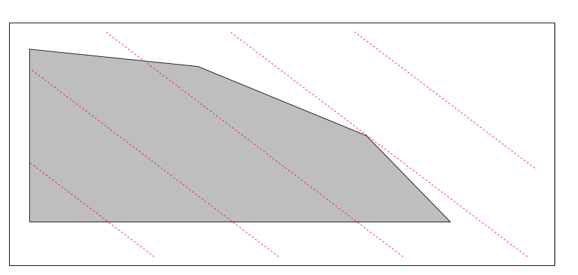
(a) Tractable problem of maximizing a linear
function over a polytope

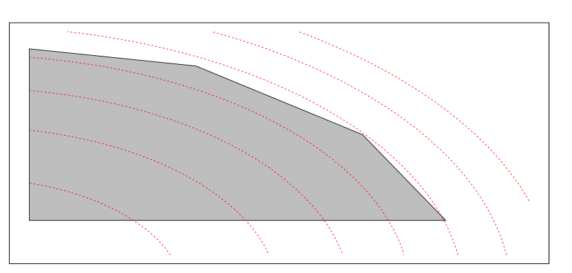
(b) Intractable problem of maximizing an upper
confidence bound over a polytope

It is worth mentioning that because posterior sampling requires specifying a fully probabilistic model of the underlying system, it may not be ideally suited for every practical setting. In particular, when dealing with some complex classes of functions, specifying an appropriate prior can be a challenge while there may be alternative algorithms that address the problem in an elegant and practically effective way.

5 Confidence Bounds and Regret Decompositions.

Unlike UCB algorithms, posterior sampling does not make use of upper confidence bounds to encourage exploration and instead relies on randomization. As such, the two classes of algorithm seem very different. However, we will establish in this section a connection that will enable us in Section 6 to derive performance bounds for posterior sampling from those that apply to UCB algorithms. Since UCB algorithms have received much more attention, this leads to a number of new results about posterior sampling. Further, the relationship yields insight into the performance advantages of posterior sampling.

5.1 UCB Regret Decomposition.

Consider a UCB algorithm with an upper confidence bound sequence $U=\{U_{t}|t\in\mathbb{N}\}$. Recall that $\bar{A}_{t}\in\arg\max_{a\in\mathcal{A}_{t}}U_{t}(a)$ and $A_{t}^{*}\in\arg\max_{a\in\mathcal{A}_{t}}f_{\theta}(a)$. We have the following simple regret decomposition:

$$f_{\theta}\left(A_{t}^{*}\right)-f_{\theta}\left(\bar{A_{t}}\right) = f_{\theta}\left(A_{t}^{*}\right)-U_{t}(\bar{A_{t}})+U_{t}(\bar{A_{t}})-f_{\theta}\left(\bar{A_{t}}\right)$$ (1)

$$\leq \left[f_{\theta}\left(A_{t}^{*}\right)-U_{t}(A_{t}^{*})\right]+\left[U_{t}(\bar{A_{t}})-f_{\theta}\left(\bar{A_{t}}\right)\right].$$

The inequality follows from the fact that $\bar{A_{t}}$ is chosen to maximize $U_{t}$. If the upper confidence bound is an upper bound with high probability, as one would expect from a UCB algorithm, then the first term is negative with high probability. The second term, $U_{t}(\bar{A_{t}})-f_{\theta}\left(\bar{A_{t}}\right)$, penalizes for the width of the confidence interval. As actions are sampled $U_{t}$ should diminish and converge on $f_{\theta}$. As such, both terms of the decomposition should eventually vanish. An important feature of this decomposition is that, so long as the first term is negative, it bounds regret in terms of uncertainty about the current action $\bar{A}_{t}$.

Taking the expectation of (1) establishes that the $T$-period Bayesian regret of a UCB algorithm satisfies

$$\text{BayesRegret}\left(T,\,\pi^{U}\right)\leq\mathbb{E}\sum_{t=1}^{T}\left[U_{t}(\bar{A_{t}})-f_{\theta}(\bar{A_{t}})\right]+\mathbb{E}\sum_{t=1}^{T}\left[f_{\theta}\left(A_{t}^{*}\right)-U_{t}(A_{t}^{*})\right],$$ (2)

where $\pi^{U}$ is the policy derived from $U$.

5.2 Posterior Sampling Regret Decomposition.

As established by the following proposition, the Bayesian regret of posterior sampling decomposes in a way analogous to what we have shown for UCB algorithms. Recall that, with some abuse of notation, for an upper confidence bound sequence $\{U_{t}|t\in\mathbb{N}\}$ we denote by $U_{t}(a)$ the random variable $U_{t}(H_{t})(a)$. The following proposition allows $U_{t}$ to be an arbitrary real valued function of $H_{t}$ and $a\in\mathcal{A}$. Let $\pi^{\rm PS}$ denote the policy followed by posterior sampling.

Proposition 5.1

For any upper confidence bound sequence $\{U_{t}|t\in\mathbb{N}\}$,

$$\textup{BayesRegret}\left(T,\,\pi^{\rm PS}\right)=\mathbb{E}\sum_{t=1}^{T}\left[U_{t}(A_{t})-f_{\theta}(A_{t})\right]+\mathbb{E}\sum_{t=1}^{T}\left[f_{\theta}\left(A_{t}^{*}\right)-U_{t}(A_{t}^{*})\right],$$ (3)

for all $T\in\mathbb{N}$.

Proof 5.2

Proof. Note that, conditioned on $H_{t}$, the optimal action $A^{*}_{t}$ and the action $A_{t}$ selected by posterior sampling are identically distributed, and $U_{t}$ is deterministic. Hence, $\mathbb{E}\left[U_{t}(A_{t}^{*})\mid H_{t}\right]=\mathbb{E}\left[U_{t}(A_{t})\mid H_{t}\right]$. Therefore

$$\mathbb{E}\left[f_{\theta}(A_{t}^{*})-f_{\theta}\left(A_{t}\right)\right] = \mathbb{E}\left[\mathbb{E}\left[f_{\theta}(A_{t}^{*})-f_{\theta}\left(A_{t}\right)\mid H_{t}\right]\right]$$

$$= \mathbb{E}\left[\mathbb{E}\left[U_{t}\left(A_{t}\right)-U_{t}\left(A_{t}^{*}\right)+f_{\theta}(A_{t}^{*})-f_{\theta}\left(A_{t}\right)\mid H_{t}\right]\right]$$

$$= \mathbb{E}\left[\mathbb{E}\left[U_{t}(A_{t})-f_{\theta}(A_{t})\mid H_{t}\right]+\mathbb{E}\left[f_{\theta}\left(A_{t}^{*}\right)-U_{t}(A_{t}^{*})\mid H_{t}\right]\right]$$

$$= \mathbb{E}\left[U_{t}(A_{t})-f_{\theta}(A_{t})\right]+\mathbb{E}\left[f_{\theta}\left(A_{t}^{*}\right)-U_{t}(A_{t}^{*})\right].$$

Summing over $t$ gives the result.

To compare (2) and (3) consider the case where $f_{\theta}$ takes values in $[0,\,C]$. Then,

$$\text{BayesRegret}\left(T,\,\pi^{U}\right)\leq\mathbb{E}\sum_{t=1}^{T}\left[U_{t}(\bar{A_{t}})-f_{\theta}(\bar{A_{t}})\right]+C\sum_{t=1}^{T}\mathbb{P}\left(f_{\theta}\left(A_{t}^{*}\right)>U_{t}(A_{t}^{*})\right)$$

and

$$\text{BayesRegret}\left(T,\,\pi^{\rm PS}\right)\leq\mathbb{E}\sum_{t=1}^{T}\left[U_{t}(A_{t})-f_{\theta}(A_{t})\right]+C\sum_{t=1}^{T}\mathbb{P}\left(f_{\theta}\left(A_{t}^{*}\right)>U_{t}(A_{t}^{*})\right).$$

An important difference to take note of is that the Bayesian regret bound of $\pi^{U}$ depends on the specific upper confidence bound sequence $U$ used by the UCB algorithm in question whereas the bound of $\pi^{\rm PS}$ applies simultaneously for all upper confidence bound sequences. This suggests that, while the Bayesian regret of a UCB algorithm depends critically on the specific choice of confidence sets, posterior sampling depends on the best possible choice of confidence sets. This is a crucial advantage when there are complicated dependencies among actions, as designing and computing with appropriate confidence sets presents significant challenges. This difficulty is likely the main reason that posterior sampling significantly outperforms recently proposed UCB algorithms in the simulations presented in Section 8.

We have shown how upper confidence bounds characterize Bayesian regret bounds for posterior sampling. We will leverage this concept in the next two sections. Let us emphasize, though, that while our analysis of posterior sampling will make use of upper confidence bounds, the actual performance of posterior sampling does not depend on upper confidence bounds used in the analysis.

6 From UCB to Posterior Sampling Regret Bounds.

In this section we present Bayesian regret bounds for posterior sampling that can be derived by combining our regret decomposition (3) with results from prior work on UCB regret bounds. Each UCB regret bound was established through a common procedure, which entailed specifying lower and upper confidence bounds $L_{t}:\mathcal{A}\mapsto\mathbb{R}$ and $U_{t}:\mathcal{A}\mapsto\mathbb{R}$ so that $L_{t}(a)\leq f_{\theta}(a)\leq U_{t}(a)$ with high probability for each $t$ and $a$, and then providing an expression that dominates the sum $\sum_{1}^{T}(U_{t}-L_{t})(a_{t})$ for all sequences of actions $a_{1},..,a_{T}$. As we will show, each such analysis together with our regret decomposition (3) leads to a Bayesian regret bound for posterior sampling.

6.1 Finitely Many Actions.

We consider in this section a problem with $|\mathcal{A}|<\infty$ actions and rewards satisfying $R_{t}\in[0,1]$ for all $t$ almost surely. We note, however, that the results we discuss can be extended to cases where $R_{t}$ is not bounded but where instead its distribution is “light-tailed.” It is also worth noting that we make no further assumptions on the class of reward functions $\mathcal{F}$ or on the prior distribution over $\theta$.

In this setting, Algorithm 1, which was proposed by Auer et al. [9], is known to satisfy a problem-independent regret bound of order $\sqrt{|\mathcal{A}|T\log T}$. Under an additional assumption that action rewards are independent and take values in $\{0,1\}$, an order $\sqrt{|\mathcal{A}|T\log T}$ regret bound for posterior sampling is also available [5].

Here we provide a Bayesian regret bound that is also of order $\sqrt{|\mathcal{A}|T\log T}$ but does not require that action rewards are independent or binary. Our analysis, like that of Auer et al. [9], makes use of confidence sets that are Cartesian products of action-specific confidence intervals. The regret decomposition (3) lets us use such confidence sets to produce bounds for posterior sampling even when the algorithm itself may exploit dependencies among actions.

Proposition 6.1

If $|\mathcal{A}|=K<\infty$ and $R_{t}\in[0,1]$, then for any $T\in\mathbb{N}$

$$\mathrm{BayesRegret}(T,\pi^{\mathrm{PS}})\leq 2\min\{K,T\}+4\sqrt{KT(2+6\log(T))}.$$ (4)

Proof 6.2

Proof. Let $N_{t}(a)=\sum_{l=1}^{t}\mathbf{1}(A_{t}=a)$ denote the number of times $a$ is sampled over the first $t$ periods, and $\hat{\mu}_{t}(a)=N_{t}(a)^{-1}\sum_{l=1}^{t}\mathbf{1}(A_{t}=a)R_{t}$ denote the empirical average reward from these samples. Define upper and lower confidence bounds as follows:

$$U_{t}(a)=\min\left\{\hat{\mu}_{t-1}(a)+\sqrt{\frac{2+6\log(T)}{N_{t-1}(a)}},1\right\} L_{t}(a)=\max\left\{\hat{\mu}_{t-1}(a)-\sqrt{\frac{2+6\log(T)}{N_{t-1}(a)}},0\right\}.$$ (5)

The next lemma, which is a consequence of analysis in Abbasi-Yadkori et al. [2], shows these hold with high probability. Were actions sampled in an iid fashion, this lemma would follow immediately from the Hoeffding inequality. For more details, see Appendix 10.

Lemma 6.3

If $U_{t}(a)$ and $L_{t}(a)$ are defined as in (5), then $\mathbb{P}\left(\bigcup_{t=1}^{T}\{f_{\theta}(a)\notin[L_{t}(a),U_{t}(a)]\}\right)\leq 1/T$.

First consider the case where $T\leq K$. Since $f_{\theta}(a)\in[0,1]$, $\mathrm{BayesRegret}(T,\pi^{\rm PS})\leq T=\min\{K,T\}$.

Now, assume $T>K$. Then,

$$\mathrm{BayesRegret}(T,\pi^{\mathrm{PS}}) \leq \mathbb{E}\left[\sum_{t=1}^{T}(U_{t}-L_{t})(A_{t})\right]+T\mathbb{P}\left(\bigcup_{a\in\mathcal{A}}\bigcup_{t=1}^{T}\left\{f_{\theta}(a)\notin[L_{t}(a),U_{t}(a)]\right\}\right)$$

$$\leq \mathbb{E}\left[\sum_{t=1}^{T}(U_{t}-L_{t})(A_{t})\right]+K.$$

We now turn to bounding $\sum_{t=1}^{T}(U_{t}-L_{t})(A_{t})$. Let $\mathcal{T}_{a}=\left\{t\leq T:A_{t}=a\right\}$ denote the periods in which $a$ is selected. Then, $\sum_{t=1}^{T}(U_{t}-L_{t})(A_{t})=\sum_{a\in\mathcal{A}}\sum_{t\in\mathcal{T}_{a}}(U_{t}-L_{t})(a)$. We show,

$$\sum_{t\in\mathcal{T}_{a}}(U_{t}-L_{t})(a)\leq 1+2\sqrt{2+6\log(T)}\sum_{t\in\mathcal{T}_{a}}(1+N_{t-1}(a))^{-1/2}=1+2\sqrt{2+6\log(T)}\sum_{j=0}^{N_{T}(a)-1}(j+1)^{-1/2}$$

and

$$\sum_{j=0}^{N_{T}(a)-1}(j+1)^{-1/2}\leq\intop_{x=0}^{N_{T}(a)}x^{-1/2}dx=2\sqrt{N_{T}(a)}.$$

Summing over actions and applying the cauchy-shwartz inequality yields,

$$\mathrm{BayesRegret}(T,\pi^{\rm PS})\leq 2K+4\sqrt{2+6\log(T)}\sum_{a\in\mathcal{A}}\sqrt{N_{T}(a)} \overset{(a)}{\leq} 2K+4\sqrt{(2+6\log(T))K\sum_{a}N_{T}(a)}$$

$$= 2K+4\sqrt{KT(2+6\log(T))}$$

$$\overset{(b)}{=} 2\min\{K,T\}+4\sqrt{KT(2+6\log(T))},$$

where (a) follows from the cauchy-shwartz inequality and (b) follows from the assumption that $T>K$.

6.2 Linear and Generalized Linear Models.

We now consider function classes that represent linear and generalized linear models. The bound of Proposition 6.1 applies so long as the number of actions is finite, but we will establish alternative bounds that depend on the dimension of the function class rather than the number of actions. Such bounds accommodate problems with infinite action sets and can be much stronger than the bound of Proposition 6.1 if there are many actions.

The Bayesian regret bounds we provide in this section derive from regret bounds of the UCB literature. In Section 7, we will establish a Bayesian regret bound that is as strong for the case of linear models and stronger for the case of generalized linear models. Since the results of Section 7 to a large extent supersede those we present here, we aim to be brief and avoid formal proofs in this section’s discussion of the bounds and how they follow from results in the literature.

6.2.1 Linear Models

In the “linear bandit” problem studied by [17, 31, 2, 3], reward functions are parameterized by a vector $\theta\in\Theta\subset\mathbb{R}^{d}$, and there is a known feature mapping $\phi:\mathcal{A}\mapsto\mathbb{R}^{d}$ such that $f_{\theta}(a)=\left\langle\phi(a),\theta\right\rangle$. The following proposition establishes Bayesian regret bounds for such problems. The proposition uses the term $\sigma$-sub-Gaussian to describe any random variable $X$ that satisfies $\mathbb{E}\exp(\lambda X)\leq\exp(\lambda^{2}\sigma^{2}/2)$ for all $\lambda\in\mathbb{R}$.

Proposition 6.4

Fix positive constants $\sigma$, $c_{1}$, and $c_{2}$. If $\Theta\subset\mathbb{R}^{d}$, $f_{\theta}(a)=\left\langle\phi(a),\theta\right\rangle$ for some $\phi:\mathcal{A}\mapsto\mathbb{R}$, $\sup_{\rho\in\Theta}\|\rho\|_{2}\leq c_{1}$, and $\sup_{a\in\mathcal{A}}\|\phi(a)\|_{2}\leq c_{2}$, and for each $t$, $R_{t}-f_{\theta}(A_{t})$ conditioned on $(H_{t},A_{t},\theta)$ is $\sigma$-sub-Gaussian, then

$${\rm BayesRegret}\left(T,\,\pi^{\rm PS}\right)=O(d\log T\sqrt{T}),$$

and

$${\rm BayesRegret}\left(T,\,\pi^{\rm PS}\right)=\tilde{O}\left(\mathbb{E}\sqrt{\left\|\theta\right\|_{0}dT}\right).$$

The second bound essentially replaces the dependence on the dimension $d$ with one on $\mathbb{E}\sqrt{\left\|\theta\right\|_{0}d}$. The “zero-norm” $\left\|\theta\right\|_{0}$ is the number of nonzero components, which can be much smaller than $d$ when the reward function admits a sparse representation. Note that $\tilde{O}$ ignores logarithmic factors. Both bounds follow from our regret decomposition (3) together with the analysis of [2], in the case of the first bound, and the analysis of [3], in the case of the second bound. We now provide a brief sketch of how these bounds can be derived.

If $f_{\theta}$ takes values in $[-C,\,C]$ then (3) implies

$$\text{BayesRegret}\left(T,\,\pi^{\rm PS}\right)\leq\mathbb{E}\sum_{t=1}^{T}\left[U_{t}(A_{t})-L_{t}(A_{t})\right]+2C\sum_{t=1}^{T}\left[\mathbb{P}\left(f_{\theta}(A^{*}_{t})>U_{t}(A^{*}_{t})\right)+\mathbb{P}\left(f_{\theta}(A_{t})<L_{t}(A_{t})\right)\right].$$ (6)

The analyses of [2] and [3] follow two steps that can be used to bound the right hand side of this equation. In the first step, an ellipsoidal confidence set $\Theta_{t}:=\{\rho\in\mathbb{R}^{d}:\|\rho-\hat{\theta}_{t}\|_{V_{t}}\leq\sqrt{\beta_{t}}\}$ is constructed, where for some $\lambda\in\mathbb{R}$, $V_{t}:=\sum_{k=1}^{t}\phi(A_{t})\phi(A_{t})^{T}+\lambda I$ captures the amount of exploration carried out in each direction up to time $t$. The upper and lower bounds induced by the ellipsoid are $U_{t}(a):=\max\left\{C,\max_{\rho\in\Theta_{t}}\left(\rho^{T}\phi(a)\right)\right\}$ and $L_{t}(a):=\min\left\{-C,\min_{\rho\in\Theta_{t}}\left(\rho^{T}\phi(a)\right)\right\}$. If the sequence of confidence parameters $\beta_{1},\ldots,\beta_{T}$ is selected so that $\mathbb{P}(\theta\notin\Theta_{t}|H_{t})\leq 1/T$ then the second term of the regret decomposition is less than $4C$. For these confidence sets, the second step establishes a bound on $\sum_{1}^{T}(U_{t}-L_{t})(a_{t})$ that holds for any sequence of actions. The analyses presented on pages 7-8 of [17] and pages 14-15 of [2] each implies such a bound of order $\sqrt{d\max_{t\leq T}\beta_{t}T\log(T/\lambda)}$. Plugging in closed form expressions for $\beta_{t}$ provided in these papers leads to the bounds of Proposition 6.4.

6.2.2 Generalized Linear Models

In a generalized linear model, the reward function takes the form $f_{\theta}(a):=g\left(\left\langle\phi(a),\theta\ \right\rangle\right)$ where the inverse link function $g$ is strictly increasing and continuously differentiable. The analysis of [18] can be applied to establish a Bayesian regret bound for posterior sampling, but with one caveat. The algorithm considered in [18] begins by selecting a sequence of actions $a_{1},..,a_{d}$ with linearly independent feature vectors $\phi(a_{1}),\ldots,\phi(a_{d})$. Until now, we haven’t even assumed such actions exist or that they are guaranteed to be feasible over the first $d$ time periods. After this period of designed exploration, the algorithm selects at each time an action that maximizes an upper confidence bound. What we will establish using the results from [18] is a bound on a similarly modified version of posterior sampling, in which the first $d$ actions taken are $a_{1},\ldots,a_{d}$, while subsequent actions are selected by posterior sampling. Note that the posterior distribution employed at time $d+1$ is conditioned on observations made over the first $d$ time periods. We denote this modified posterior sampling algorithm by $\pi^{\rm IPS}_{a_{1},\ldots,a_{d}}$. It is worth mentioning here that in Section 7 we present a result with a stronger bound that applies to the standard version of posterior sampling, which does not include a designed exploration period.

Proposition 6.5

Fix positive constants $c_{1}$, $c_{2}$, $C$, and $\lambda$. If $\Theta\subset\mathbb{R}^{d}$, $f_{\theta}(a)=g(\left\langle\phi(a),\theta\right\rangle)$ for some strictly increasing continuously differentiable function $g:\mathbb{R}\mapsto\mathbb{R}$, $\sup_{\rho\in\Theta}\|\rho\|_{2}\leq c_{1}$, $\sup_{a\in\mathcal{A}}\|\phi(a)\|_{2}\leq c_{2}$, $\mathcal{A}_{t}=\mathcal{A}$ for all $t$, $\sum_{i=1}^{d}\phi(a_{i})\phi(a_{i})^{T}\succeq\lambda I$ for some $a_{1},\ldots,a_{d}\in\mathcal{A}$, and $R_{t}\in[0,C]$ for all $t$, then

$${\rm BayesRegret}\left(T,\,\pi^{\rm IPS}_{a_{1},\ldots,a_{d}}\right)=O(rd\log^{3/2}T\sqrt{T}),$$

where $r=\sup_{\rho,a}g^{\prime}(\langle\phi(a),\rho\rangle)/\inf_{\rho,a}g^{\prime}(\langle\phi(a),\rho\rangle)$.

Like the analyses of [2] and [3], which apply to linear models, the analysis of [18] follows two steps that together bound both terms of our regret decomposition (6). First, an ellipsoidal confidence set $\Theta_{t}$ is constructed, centered around a quasi-maximum likelihood estimator. This confidence set is designed to contain $\theta$ with high probability. Given confidence bounds $U_{t}(a):=\max\{C,\max_{\rho\in\Theta_{t}}g(\langle\phi(a),\rho\rangle)\}$ and $L_{t}(a):=\min\{0,\min_{\rho\in\Theta_{t}}g(\langle\phi(a),\rho\rangle)\}$, a worst case bound on $\sum_{1}^{T}(U_{t}-L_{t})(a_{t})$ is established. The bound is similar to those established for the linear case, but there is an added dependence on the the slope of $g$.

6.3 Gaussian Processes.

In this section we consider the case where the reward function $f_{\theta}$ is sampled from a Gaussian process. That is, the stochastic process $\left(f_{\theta}(a):a\in\mathcal{A}\right)$ is such that for any $a_{1},..,a_{k}\in\mathcal{A}$ the collection $f_{\theta}(a_{1}),..,f_{\theta}(a_{k})$ follows a multivariate Gaussain distribution. Srinivas et al. [35] study a UCB algorithm designed for such problems and provide general regret bounds. Again, through the regret decomposition (3) their analysis provides a Bayesian regret bound for posterior sampling.

For simplicity, we focus our discussion on the case where $\mathcal{A}$ is finite, so that $\left(f_{\theta}(a):a\in\mathcal{A}\right)$ follows a multivariate Gaussian distribution. As shown by Srinivas et al. [35], the results extend to infinite action sets through a discretization argument as long as certain smoothness conditions are satisfied.

When confidence bounds hold, a UCB algorithm incurs high regret from sampling an action only when the confidence bound at that action is loose. In that case, one would expect the algorithm to learn a lot about $f_{\theta}$ based on the observed reward. This suggests the algorithm’s cumulative regret may be bounded in an appropriate sense by the total amount it is expected to learn. Leveraging the structure of the Gaussian distribution, Srinivas et al. [35] formalize this idea. They bound the regret of their UCB algorithm in terms of the maximum amount that any algorithm could learn about $f_{\theta}$. They use an information theoretic measure of learning: the information gain. This is defined to be the difference between the entropy of the prior distribution of $\left(f_{\theta}(a):a\in\mathcal{A}\right)$ and the entropy of the posterior. The maximum possible information gain is denoted $\gamma_{T}$, where the maximum is taken over all sequences $a_{1},..,a_{T}$. Their analysis also supports the following result on posterior sampling.

Proposition 6.6

If $\mathcal{A}$ is finite, $\left(f_{\theta}(a):a\in\mathcal{A}\right)$ follows a multivariate Gaussian distribution with marginal variances bounded by $1$, $R_{t}-f_{\theta}(A_{t})$ is independent of $(H_{t},\theta,A_{t})$, and $\{R_{t}-f_{\theta}(A_{t})|t\in\mathbb{N}\}$ is an iid sequence of zero-mean Gaussian random variables with variance $\sigma^{2}$, then

$${\rm BayesRegret}\left(T,\,\pi^{\rm PS}\right)\leq 1+2\sqrt{T\gamma_{T}\ln\left(1+\sigma^{-2}\right)^{-1}\ln\left(\frac{(T^{2}+1)\left|\mathcal{A}\right|}{\sqrt{2\pi}}\right)}$$

for all $T\in\mathbb{N}$.

Srinivas et al. [35] also provide bounds on $\gamma_{T}$ for kernels commonly used in Gaussian process regression, including the linear kernel, radial basis kernel, and Matérn kernel. Combined with the above proposition, this yields explicit Bayesian regret bounds in these cases.

We will briefly comment on their analysis and how it provides a bound for posterior sampling. First, note that the posterior distribution is Gaussian, which suggests an upper confidence bound of the form $U_{t}(a):=\mu_{t-1}(a)+\sqrt{\beta_{t}}\sigma_{t-1}(a)$, where $\mu_{t-1}(a)$ is the posterior mean, $\sigma_{t-1}(a)$ is the posterior standard deviation of $f_{\theta}(a)$, and $\beta_{t}$ is a confidence parameter. We can provide a Bayesian regret bound by bounding both terms of (3). The next lemma, which follows, bounds the second term. Some new analysis is required since the Gaussian distribution is unbounded, and we study Bayesian regret whereas Srinivas et al. [35] bound regret with high probability under the prior.

Lemma 6.7

If $U_{t}(a):=\mu_{t-1}(a)+\sqrt{\beta_{t}}\sigma_{t-1}(a)$ and $\beta_{t}:=2\ln\left(\frac{\left(t^{2}+1\right)\left|\mathcal{A}\right|}{\sqrt{2\pi}}\right)$ then for all $T\in\mathbb{N}$ $\mathbb{E}\sum_{t=1}^{T}\left[f_{\theta}\left(A_{t}^{*}\right)-U_{t}(A_{t}^{*})\right]\leq 1.$

Proof 6.8

Proof. First, if $X\sim N(\mu,\sigma^{2})$ then if $\mu\leq 0$, $\mathbb{E}\left[X{\bf 1}\left\{X>0\right\}\right]=\intop_{0}^{\infty}\frac{x}{\sigma\sqrt{2\pi}}\exp\left\{\frac{-(x-\mu)^{2}}{2\sigma^{2}}\right\}dx=\frac{\sigma}{\sqrt{2\pi}}\exp\left\{\frac{-\mu^{2}}{2\sigma^{2}}\right\}.$

Then since the posterior distribution of $f_{\theta}(a)-U_{t}(a)$ is normal with mean $-\sqrt{\beta_{t}}\sigma_{t-1}(a)$ and variance $\sigma^{2}_{t-1}(a)$

$$\mathbb{E}\left[\mathbf{1}\left\{f_{\theta}(a)-U_{t}(a)\geq 0\right\}\left[f_{\theta}(a)-U_{t}(a)\right]|H_{t}\right]=\frac{\sigma_{t-1}(a)}{\sqrt{2\pi}}\exp\left\{\frac{-\beta_{t}}{2}\right\}=\frac{\sigma_{t-1}(a)}{\left(t^{2}+1\right)\left|\mathcal{A}\right|}\leq\frac{1}{\left(t^{2}+1\right)\left|\mathcal{A}\right|}.$$ (7)

The final inequality above follows from the assumption that $\sigma_{0}(a)\leq 1$. The claim follows from (7) since

$$\mathbb{E}\sum_{t=1}^{T}\left[f_{\theta}(A_{t}^{*})-U_{t}(A_{t}^{*})\right]\leq\sum_{t=1}^{\infty}\sum_{a\in\mathcal{A}}\mathbb{E}\left[\mathbf{1}\left\{f_{\theta}(a)-U_{t}(a)\geq 0\right\}\left[f_{\theta}(a)-U_{t}(a)\right]\right]\leq\sum_{t=1}^{\infty}\frac{1}{\left(t^{2}+1\right)}\leq 1.\Halmos$$

Now, consider the first term of (3), which is:

$$\mathbb{E}\sum_{t=1}^{T}(U_{t}-f_{\theta})(A_{t})=\mathbb{E}\sum_{t=1}^{T}(U_{t}-\mu_{t-1})(A_{t})=\mathbb{E}\sum_{t=1}^{T}\sqrt{\beta_{t}}\sigma_{t-1}(A_{t})\leq\mathbb{E}\sqrt{T\max_{t\leq T}\beta_{t}}\sqrt{\sum_{t=1}^{T}{\sigma^{2}_{t-1}(A_{t})}}.$$

Here the second equality follows by the tower property of conditional expectation, and the final step follows from the Cauchy-Schwartz inequality. Therefore, to establish a Bayesian regret bound it is sufficient to provide a bound on the sum of posterior variances $\sum_{t=1}^{T}{\sigma^{2}_{t-1}(a_{t})}$ that holds for any $a_{1},..,a_{T}$. Under the assumption that $\sigma_{0}(a)\leq 1$, the proof of Lemma 5.4 of Srinivas et al. [35] shows that $\sigma^{2}_{t-1}(a_{t})\leq\alpha^{-1}\log\left(1+\sigma^{-2}\sigma_{t-1}^{2}(a_{t})\right)$, where $\alpha=\left(1+\sigma^{-2}\right)$. At the same time, Lemma 5.3 of Srinivas et al. [35] shows the information gain from selecting $a_{1},...a_{T}$ is equal to $\frac{1}{2}\sum_{t=1}^{T}\log\left(1+\sigma^{-2}\sigma_{t-1}^{2}(a_{t})\right)$. This shows that for any actions $a_{1},..,a_{T}$ the the sum of posterior variances $\sum_{t=1}^{T}{\sigma^{2}_{t-1}(a_{t})}$ can be bounded in terms of the information gain from selecting $a_{1},..,a_{T}$. Therefore $\sum_{t=1}^{T}{\sigma^{2}_{t-1}(A_{t})}$ can be bounded in terms of the largest possible information gain $\gamma_{T}$.

7 Bounds for General Function Classes.

The previous section treated models in which the relationship among action rewards takes a simple and tractable form. Indeed, nearly all of the multi-armed bandit literature focuses on such problems. Posterior sampling can be applied to a much broader class of models. As such, more general results that hold beyond restrictive cases are of particular interest. In this section, we provide a Bayesian regret bound that applies when the reward function lies in a known, but otherwise arbitrary class of uniformly bounded real-valued functions $\mathcal{F}$. Our analysis of this abstract framework yields a more general result that applies beyond the scope of specific problems that have been studied in the literature, and also identifies factors that unify more specialized prior results. Further, our more general result when specialized to linear models recovers the strongest known Bayesian regret bound and in the case of generalized linear models yields a bound stronger than that established in prior literature.

If $\mathcal{F}$ is not appropriately restricted, it is impossible to guarantee any reasonably attractive level of Bayesian regret. For example, in a case where $\mathcal{A}=[0,1]$, $f_{\theta}(a)={\bf 1}(\theta=a)$, $\mathcal{F}=\{f_{\theta}|\theta\in[0,1]\}$, and $\theta$ is uniformly distributed over $[0,1]$, it is easy to see that the Bayesian regret of any algorithm over $T$ periods is $T$, which is no different from the worst level of performance an agent can experience.

This example highlights the fact that Bayesian regret bounds must depend on the function class $\mathcal{F}$. The bound we develop in this section depends on $\mathcal{F}$ through two measures of complexity. The first is the Kolmogorov dimension, which measures the growth rate of the covering numbers of $\mathcal{F}$ and is closely related to measures of complexity that are common in the supervised learning literature. It roughly captures the sensitivity of $\mathcal{F}$ to statistical over-fitting. The second measure is a new notion we introduce, which we refer to as the eluder dimension. This captures how effectively the value of unobserved actions can be inferred from observed samples. We highlight in Section 7.3 why notions of dimension common to the supervised learning literature are insufficient for our purposes.

Though the results of this section are very general, they do not apply to the entire range of problems represented by the formulation we introduced in Section 3. In particular, throughout the scope of this section, we fix constants $C>0$ and $\sigma>0$ and impose two simplifying assumptions. The first concerns boundedness of reward functions. For all $f\in\mathcal{F}$ and $a\in\mathcal{A}$, $f(a)\in[0,C]$. Our second assumption ensures that observation noise is light-tailed. Recall that we say a random variable $x$ is $\sigma$-sub-Gaussian if $\mathbb{E}[\exp(\lambda x)]\leq\exp(\lambda^{2}\sigma^{2}/2)$ almost surely for all $\lambda$. For all $t\in\mathbb{N}$, $R_{t}-f_{\theta}(A_{t})$ conditioned on $(H_{t},\theta,A_{t})$ is $\sigma$-sub-Gaussian. It is worth noting that the Bayesian regret bounds we provide are distribution independent, in the sense that we show $\mathrm{BayesRegret}(T,\pi^{\mathrm{PS}})$ is bounded by an expression that does not depend on $\mathbb{P}(\theta\in\cdot)$.

Our analysis in some ways parallels those found in the literature on UCB algorithms. In the next section we provide a method for constructing a set $\mathcal{F}_{t}\subset\mathcal{F}$ of functions that are statistically plausible at time $t$. Let $w_{\mathcal{F}}(a):=\sup_{\overline{f}\in\mathcal{F}}\overline{f}(a)-\inf_{\underline{f}\in\mathcal{F}}\underline{f}(a)$ denote the width of $\mathcal{F}$ at $a$. Based on these confidence sets, and using the regret decomposition (3), one can bound Bayesian regret in terms of $\sum_{1}^{T}w_{\mathcal{F}_{t}}(A_{t})$. In Section 7.2, we establish a bound on this sum in terms of the Kolmogorov and eluder dimensions of $\mathcal{F}$.

7.1 Confidence Bounds.

The construction of tight confidence sets for specific classes of functions presents technical challenges. Even for the relatively simple case of linear bandit problems, significant analysis is required. It is therefore perhaps surprising that, as we show in this section, one can construct strong confidence sets for an arbitrary class of functions without much additional sophistication. While the focus of our work is on providing a Bayesian regret bound for posterior sampling, the techniques we introduce for constructing confidence sets may find broader use.

The confidence sets constructed here are centered around least squares estimates $\hat{f}_{t}^{LS}\in\arg\min_{f\in\mathcal{F}}L_{2,t}(f)$ where $L_{2,t}(f)=\sum_{1}^{t-1}(f(A_{t})-R_{t})^{2}$ is the cumulative squared prediction error. The sets take the form $\mathcal{F}_{t}:=\{f\in\mathcal{F}:\|f-\hat{f}_{t}^{LS}\|_{2,E_{t}}\leq\sqrt{\beta_{t}}\}$ where $\beta_{t}$ is an appropriately chosen confidence parameter, and the empirical 2-norm $\left\|\cdot\right\|_{2,E_{t}}$ is defined by $\left\|g\right\|_{2,E_{t}}^{2}=\sum_{1}^{t-1}g^{2}(A_{k})$. Hence $\left\|f-f_{\theta}\right\|_{2,E_{t}}^{2}$ measures the cumulative discrepancy between the previous predictions of $f$ and $f_{\theta}$.

The following lemma is the key to constructing strong confidence sets $\left(\mathcal{F}_{t}:t\in\mathbb{N}\right)$. For an arbitrary function $f$, it bounds the squared error of $f$ from below in terms of the empirical loss of the true function $f_{\theta}$ and the aggregate empirical discrepancy $\left\|f-f_{\theta}\right\|_{2,E_{t}}^{2}$ between $f$ and $f_{\theta}$. It establishes that for any function $f$, with high probability, the random process $(L_{2,t}(f):t\in\mathbb{N})$ never falls below the process $(L_{2,t}(f_{\theta})+\frac{1}{2}\|f-f_{\theta}\|_{2,E_{t}}^{2}:\,t\in\mathbb{N})$ by more than a fixed constant. A proof of the lemma is provided in the appendix.

Lemma 7.1

For any $\delta>0$ and $f:\mathcal{A}\mapsto\mathbb{R}$, with probability at least $1-\delta$,

$$L_{2,t}(f)\geq L_{2,t}(f_{\theta})+\frac{1}{2}\left\|f-f_{\theta}\right\|_{2,E_{t}}^{2}-4\sigma^{2}\log\left(1/\delta\right)$$

simultaneously for all $t\in\mathbb{N}$.

By Lemma 7.1, with high probability, $f$ can enjoy lower squared error than $f_{\theta}$ only if its empirical deviation $\left\|f-f_{\theta}\right\|_{2,E_{t}}^{2}$ from $f_{\theta}$ is less than $8\sigma^{2}\log(1/\delta)$. Through a union bound, this property holds uniformly for all functions in a finite subset of $\mathcal{F}$. Using this fact and a discretization argument, together with the observation that $L_{2,t}(\hat{f}_{t}^{LS})\leq L_{2,t}(f_{\theta})$, we can establish the following result, which is proved in the appendix. Let $N(\mathcal{F},\,\alpha,\,\left\|\cdot\right\|_{\infty})$ denote the $\alpha$-covering number of $\mathcal{F}$ in the sup-norm $\|\cdot\|_{\infty}$, and let

$$\beta^{*}_{t}\left(\mathcal{F},\delta,\alpha\right):=8\sigma^{2}\log\left(N(\mathcal{F},\,\alpha,\,\left\|\cdot\right\|_{\infty})/\delta\right)+2\alpha t\left(8C+\sqrt{8\sigma^{2}\ln(4t^{2}/\delta)}\right).$$ (8)

Proposition 7.2

For all $\delta>0$ and $\alpha>0$, if

$$\mathcal{F}_{t}=\left\{f\in\mathcal{F}:\,\left\|f-\hat{f}_{t}^{LS}\right\|_{2,E_{t}}\leq\sqrt{\beta^{*}_{t}\left(\mathcal{F},\delta,\alpha\right)}\right\}$$

for all $t\in\mathbb{N}$, then

$$\mathbb{P}\left(f_{\theta}\in\bigcap_{t=1}^{\infty}\mathcal{F}_{t}\right)\geq 1-2\delta.$$

While the expression (8) defining the confidence parameter is complicated, it can be bounded by simple expressions in important cases. We provide three examples.

Example 7.3

Finite function classes: When $\mathcal{F}$ is finite, $\beta^{*}_{t}(\mathcal{F},\delta,0)=8\sigma^{2}\log(\left|\mathcal{F}\right|/\delta)$.

Example 7.4

Linear Models: Consider the case of a $d$-dimensional linear model $f_{\rho}(a):=\left\langle\phi(a),\,\rho\right\rangle$. Fix $\gamma=\sup_{a\in\mathcal{A}}\|\phi(a)\|$ and $s=\sup_{\rho\in\Theta}\|\rho\|$. Hence, for all $\rho_{1},\rho_{2}\in\mathcal{F}$, we have $\|f_{\rho_{1}}-f_{\rho_{2}}\|_{\infty}\leq\gamma\|\rho_{1}-\rho_{2}\|$. An $\alpha$-covering of $\mathcal{F}$ can therefore be attained through an $(\alpha/\gamma)$-covering of $\Theta\subset\mathbb{R}^{d}$. Such a covering requires $O((1/\alpha)^{d})$ elements, and it follows that, $\log N(\mathcal{F},\,\alpha,\,\left\|\cdot\right\|_{\infty})=O(d\log(1/\alpha))$. If $\alpha$ is chosen to be $1/t^{2}$, the second term in (8) tends to zero, and therefore, $\beta_{t}^{*}(\mathcal{F},\delta,1/t^{2})=O(d\log(t/\delta))$.

Example 7.5

Generalized Linear Models: Consider the case of a $d$-dimensional generalized linear model $f_{\theta}(a):=g\left(\left\langle\phi(a),\,\theta\right\rangle\right)$ where $g$ is an increasing Lipschitz continuous function. Fix $g$, $\gamma=\sup_{a\in\mathcal{A}}\|\phi(a)\|$, and $s=\sup_{\rho\in\Theta}\|\rho\|$. Then, the previous argument shows $\log N(\mathcal{F},\,\alpha,\,\left\|\cdot\right\|_{\infty})=O(d\log(1/\alpha))$. Again, choosing $\alpha=1/t^{2}$ yields a confidence parameter $\beta_{t}^{*}(\mathcal{F},\delta,1/t^{2})=O(d\log(t/\delta))$.

The confidence parameter $\beta^{*}_{t}(\mathcal{F},1/t^{2},1/t^{2})$ is closely related to the following concept.

Definition 7.6

The Kolmogorov dimension of a function class $\mathcal{F}$ is given by

$${\rm dim}_{K}(\mathcal{F})=\underset{\alpha\downarrow 0}{\lim\sup}\frac{\log N(\mathcal{F},\,\alpha,\,\left\|\cdot\right\|_{\infty})}{\log(1/\alpha)}.$$

In particular, we have the following result.

Proposition 7.7

For any fixed class of functions $\mathcal{F}$,

$$\beta^{*}_{t}\left(\mathcal{F},1/t^{2},1/t^{2}\right)=16(1+o(1)+{\rm dim}_{K}(\mathcal{F}))\log t.$$

Proof 7.8

Proof. By definition

$$\beta^{*}_{t}\left(\mathcal{F},1/t^{2},1/t^{2}\right)=8\sigma^{2}\left[\frac{\log\left(N\left(\mathcal{F},\,1/t^{2},\,\left\|\cdot\right\|_{\infty}\right)\right)}{\log\left(t^{2}\right)}+1\right]\log\left(t^{2}\right)+2\frac{t}{t^{2}}\left(8C+\sqrt{8\sigma^{2}\ln(4t^{2}\delta)}\right)$$

The result follows from the fact that $\underset{t\rightarrow\infty}{\lim\sup}\log\left(N\left(\mathcal{F},\,1/t^{2},\,\left\|\cdot\right\|_{\infty}\right)\right)/\log\left(t^{2}\right)={\rm dim}_{K}(\mathcal{F})$.

7.2 Bayesian Regret Bounds.

In this section we introduce a new notion of complexity – the eluder dimension – and then use it to develop a Bayesian regret bound. First, we note that, using the regret decomposition (3) and the confidence sets $\left(\mathcal{F}_{t}:t\in\mathbb{N}\right)$ constructed in the previous section, we can bound the Bayesian regret of posterior sampling in terms confidence interval widths $w_{\mathcal{F}}(a):=\sup_{f\in\mathcal{F}}f(a)-\inf_{f\in\mathcal{F}}f(a)$. In particular, the following lemma follows from our regret decomposition (3).

Lemma 7.9

For all $T\in\mathbb{N}$, if $\inf_{\rho\in\mathcal{F}_{\tau}}f_{\rho}(a)\leq f_{\theta}(a)\leq\sup_{\rho\in\mathcal{F}_{\tau}}f_{\rho}(a)$ for all $\tau\in\mathbb{N}$ and $a\in\mathcal{A}$ with probability at least $1-1/T$ then

$${\rm BayesRegret}(T,\pi^{\rm PS})\leq C+\mathbb{E}\sum_{t=1}^{T}w_{\mathcal{F}_{t}}(A_{t}).$$

We can use the confidence sets constructed in the previous section to guarantee that the conditions of this lemma hold. In particular, choosing $\delta=1/2T$ in (8) guarantees that $f_{\theta}\in\bigcap_{t=1}^{\infty}\mathcal{F}_{t}$ with probability at least $1-1/T$.

Our remaining task is to provide a worst case bound on the sum $\sum_{1}^{T}w_{\mathcal{F}_{t}}(A_{t})$. First consider the case of a linearly parameterized model where $f_{\rho}(a):=\left\langle\phi(a),\,\rho\right\rangle$ for each $\rho\in\Theta\subset\mathbb{R}^{d}$. Then, it can be shown that our confidence set takes the form $\mathcal{F}_{t}:=\left\{f_{\rho}:\rho\in\Theta_{t}\right\}$ where $\Theta_{t}\subset\mathbb{R}^{d}$ is an ellipsoid. When an action $A_{t}$ is sampled, the ellipsoid shrinks in the direction $\phi(A_{t})$. Here the explicit geometric structure of the confidence set implies that the width $w_{\mathcal{F}_{t}}$ shrinks not only at $A_{t}$ but also at any other action whose feature vector is not orthogonal to $\phi(A_{t})$. Some linear algebra leads to a worst case bound on $\sum_{1}^{T}w_{\mathcal{F}_{t}}(A_{t})$. For a general class of functions, the situation is much subtler, and we need to measure the way in which the width at each action can be reduced by sampling other actions. To do this, we introduce the following notion of dependence.

Definition 7.10

An action $a\in\mathcal{A}$ is $\epsilon$-dependent on actions $\{a_{1},...,a_{n}\}\subseteq\mathcal{A}$ with respect to $\mathcal{F}$ if any pair of functions $f,\tilde{f}\in\mathcal{F}$ satisfying $\sqrt{\sum_{i=1}^{n}(f(a_{i})-\tilde{f}(a_{i}))^{2}}\leq\epsilon$ also satisfies $f(a)-\tilde{f}(a)\leq\epsilon$. Further, $a$ is $\epsilon$-independent of $\left\{a_{1},..,a_{n}\right\}$ with respect to $\mathcal{F}$ if $a$ is not $\epsilon$-dependent on $\left\{a_{1},..,a_{n}\right\}$.

Intuitively, an action $a$ is independent of $\{a_{1},...,a_{n}\}$ if two functions that make similar predictions at $\{a_{1},...,a_{n}\}$ can nevertheless differ significantly in their predictions at $a$. The above definition measures the “similarity” of predictions at $\epsilon$-scale, and measures whether two functions make similar predictions at $\{a_{1},...,a_{n}\}$ based on the cumulative discrepancy $\sqrt{\sum_{i=1}^{n}(f(a_{i})-\tilde{f}(a_{i}))^{2}}$. This measure of dependence suggests using the following notion of dimension. In this definition, we imagine that the sequence of elements in $\mathcal{A}$ is chosen by an eluder who hopes to show the agent poorly understood actions for as long as possible.

Definition 7.11

The $\epsilon$-eluder dimension ${\rm dim}_{E}(\mathcal{F},\epsilon)$ is the length $d$ of the longest sequence of elements in $\mathcal{A}$ such that, for some $\epsilon^{\prime}\geq\epsilon$, every element is $\epsilon^{\prime}$-independent of its predecessors.

Recall that a vector space has dimension $d$ if and only if $d$ is the length of the longest sequence of elements such that each element is linearly independent or equivalently, $0$-independent of its predecessors. Definition 7.11 replaces the requirement of linear independence with $\epsilon$-independence. This extension is advantageous as it captures both nonlinear dependence and approximate dependence. The following result uses our new notion of dimension to bound the number of times the width of the confidence interval for a selected action $A_{t}$ can exceed a threshold.

Proposition 7.12

If $(\beta_{t}\geq 0|t\in\mathbb{N})$ is a nondecreasing sequence and $\mathcal{F}_{t}:=\{f\in\mathcal{F}:\,\|f-\hat{f}_{t}^{LS}\|_{2,E_{t}}\leq\sqrt{\beta_{t}}\}$ then

$$\sum_{t=1}^{T}{\bf 1}(w_{\mathcal{F}_{t}}(A_{t})>\epsilon)\leq\left(\frac{4\beta_{T}}{\epsilon^{2}}+1\right){\rm dim}_{E}(\mathcal{F},\epsilon)$$

for all $T\in\mathbb{N}$ and $\epsilon>0$.

Proof 7.13

Proof. We begin by showing that if $w_{t}(A_{t})>\epsilon$ then $A_{t}$ is $\epsilon$-dependent on fewer than $4\beta_{T}/\epsilon^{2}$ disjoint subsequences of $(A_{1},..,A_{t-1})$, for $T>t$. To see this, note that if $w_{\mathcal{F}_{t}}(A_{t})>\epsilon$ there are $\bar{f},\,\underline{f}\,\in\mathcal{F}_{t}$ such that $\overline{f}(A_{t})-\underline{f}(A_{t})>\epsilon$. By definition, since $\overline{f}(A_{t})-\underline{f}(A_{t})>\epsilon$, if $A_{t}$ is $\epsilon$-dependent on a subsequence $(A_{i_{1}},..,\,A_{i_{k}})$ of $(A_{1},..,A_{t-1})$ then $\sum_{j=1}^{k}(\overline{f}(A_{i_{j}})-\underline{f}(A_{i_{j}}))^{2}>\epsilon^{2}$. It follows that, if $A_{t}$ is $\epsilon$-dependent on $K$ disjoint subsequences of $(A_{1},..,A_{t-1})$ then $\|\overline{f}-\underline{f}\|_{2,E_{t}}^{2}>K\epsilon^{2}$. By the triangle inequality, we have

$$\left\|\overline{f}-\underline{f}\right\|_{2,E_{t}}\leq\left\|\overline{f}-\hat{f}^{LS}_{t}\right\|_{2,E_{t}}+\left\|\underline{f}-\hat{f}^{LS}_{t}\right\|_{2,E_{t}}\leq 2\sqrt{\beta_{t}}\leq 2\sqrt{\beta_{T}}.$$

and it follows that $K<4\beta_{T}/\epsilon^{2}$.

Next, we show that in any action sequence $(a_{1},..,a_{\tau})$, there is some element $a_{j}$ that is $\epsilon$-dependent on at least $\tau/d-1$ disjoint subsequences of $\left(a_{1},..,a_{j-1}\right)$, where $d:={\rm dim}_{E}(\mathcal{F},\epsilon)$. To show this, for an integer $K$ satisfying $Kd+1\leq\tau\leq Kd+d$, we will construct $K$ disjoint subsequences $B_{1},\ldots,B_{K}$. First let $B_{i}=\left(a_{i}\right)$ for $i=1,..,K$. If $a_{K+1}$ is $\epsilon$-dependent on each subsequence $B_{1},..,B_{K}$, our claim is established. Otherwise, select a subsequence $B_{i}$ such that $a_{K+1}$ is $\epsilon$-independent and append $a_{K+1}$ to $B_{i}$. Repeat this process for elements with indices $j>K+1$ until $a_{j}$ is $\epsilon$-dependent on each subsequence or $j=\tau$. In the latter scenario $\sum|B_{i}|\geq Kd$, and since each element of a subsequence $B_{i}$ is $\epsilon$-independent of its predecessors, $|B_{i}|=d$. In this case, $a_{\tau}$ must be $\epsilon$–dependent on each subsequence.

Now consider taking $(a_{1},..,a_{\tau})$ to be the subsequence $(A_{t_{1}},\ldots,A_{t_{\tau}})$ of $(A_{1},\ldots,A_{T})$ consisting of elements $A_{t}$ for which $w_{\mathcal{F}_{t}}(A_{t})>\epsilon$. As we have established, each $A_{t_{j}}$ is $\epsilon$-dependent on fewer than $4\beta_{T}/\epsilon^{2}$ disjoint subsequences of $(A_{1},..,A_{t_{j}-1})$. It follows that each $a_{j}$ is $\epsilon$-dependent on fewer than $4\beta_{T}/\epsilon^{2}$ disjoint subsequences of $(a_{1},..,a_{j-1})$. Combining this with the fact we have established that there is some $a_{j}$ that is $\epsilon$-dependent on at least $\tau/d-1$ disjoint subsequences of $\left(a_{1},..,a_{j-1}\right)$, we have $\tau/d-1\leq 4\beta_{T}/\epsilon^{2}$. It follows that $\tau\leq(4\beta_{T}/\epsilon^{2}+1)d$, which is our desired result.

Using Proposition 7.12, one can bound the sum $\sum_{t=1}^{T}w_{\mathcal{F}_{t}}(A_{t})$, as established by the following lemma.

Lemma 7.14

If $(\beta_{t}\geq 0|t\in\mathbb{N})$ is a nondecreasing sequence and $\mathcal{F}_{t}:=\{f\in\mathcal{F}:\,\|f-\hat{f}_{t}^{LS}\|_{2,E_{t}}\leq\sqrt{\beta_{t}}\}$ then

$$\sum_{t=1}^{T}w_{\mathcal{F}_{t}}(A_{t})\leq 1+\dim_{E}\left(\mathcal{F},T^{-1}\right)C+4\sqrt{\dim_{E}\left(\mathcal{F},T^{-1}\right)\beta_{T}T}$$

for all $T\in\mathbb{N}$.

Proof 7.15

Proof. To reduce notation, write $d=\dim_{E}\left(\mathcal{F},T^{-1}\right)$ and $w_{t}=w_{t}(A_{t})$. Reorder the sequence $\left(w_{1},...,w_{T}\right)\rightarrow\left(w_{i_{1}},...,w_{i_{T}}\right)$ where $w_{i_{1}}\geq w_{i_{2}}\geq...\geq w_{i_{T}}$. We have

$$\sum_{t=1}^{T}w_{\mathcal{F}_{t}}(A_{t})=\sum_{t=1}^{T}w_{i_{t}}=\sum_{t=1}^{T}w_{i_{t}}\mathbf{1}\left\{w_{i_{t}}\leq T^{-1}\right\}+\sum_{t=1}^{T}w_{i_{t}}\mathbf{1}\left\{w_{i_{t}}>T^{-1}\right\}\leq 1+\sum_{t=1}^{T}w_{i_{t}}\mathbf{1}\left\{w_{i_{t}}\geq T^{-1}\right\}.$$

We know $w_{i_{t}}\leq C$. In addition, $w_{i_{t}}>\epsilon\iff\sum_{k=1}^{T}\mathbf{1}\left(w_{\mathcal{F}_{k}}\left(A_{k}\right)>\epsilon\right)\geq t$. By Proposition 7.12, this can only occur if $t<\left(\frac{4\beta_{T}}{\epsilon^{2}}+1\right)\dim_{E}(\mathcal{F},\epsilon)$. For $\epsilon\geq T^{-1}$, $\dim_{E}(\mathcal{F},\epsilon)\leq\dim_{E}(\mathcal{F},T^{-1})=d$, since $\dim_{E}\left(\mathcal{F},\epsilon^{\prime}\right)$ is nonincreasing in $\epsilon^{\prime}$. Therefore, when $w_{i_{t}}>\epsilon\geq T^{-1}$, $t<\left(\frac{4\beta_{T}}{\epsilon^{2}}+1\right)d$ which implies $\epsilon<\sqrt{\frac{4\beta_{T}d}{t-d}}$. This shows that if $w_{i_{t}}>T^{-1}$, then $w_{i_{t}}\leq\min\left\{C,\sqrt{\frac{4\beta_{T}d}{t-d}}\right\}$. Therefore,

$$\sum_{t=1}^{T}w_{i_{t}}\mathbf{1}\left\{w_{i_{t}}>T^{-1}\right\}\leq dC+\sum_{t=d+1}^{T}\sqrt{\frac{4d\beta_{T}}{t-d}}\leq dC+2\sqrt{d\beta_{T}}\intop_{t=0}^{T}\frac{1}{\sqrt{t}}dt=dC+4\sqrt{d\beta_{T}T}\Halmos$$

Our next result, which follows from Lemma 7.9, Lemma 7.14, and Proposition 7.2, establishes a Bayesian regret bound.

Proposition 7.16

For all $T\in\mathbb{N}$, $\alpha>0$ and $\delta\leq 1/2T$,

$${\rm BayesRegret}\left(T,\,\pi^{\rm PS}\right)\leq 1+\left[{\rm dim}_{E}\left(\mathcal{F},T^{-1}\right)+1\right]C+4\sqrt{{\rm dim}_{E}\left(\mathcal{F},T^{-1}\right)\beta^{*}_{T}\left(\mathcal{F},\alpha,\delta\right)T}.$$

Using bounds on $\beta_{t}^{*}$ provided in the previous section together with Proposition 7.16 yields Bayesian regret bounds that depend on $\mathcal{F}$ only through the eluder dimension and either the cardinality or Kolmogorov dimension. The following proposition provides such bounds.

Proposition 7.17

For any fixed class of functions $\mathcal{F}$,

$${\rm BayesRegret}\left(T,\,\pi^{\rm PS}\right)\leq 1+\left[{\rm dim}_{E}\left(\mathcal{F},T^{-1}\right)+1\right]C+16\sigma\sqrt{{\rm dim}_{E}\left(\mathcal{F},T^{-1}\right)\left(1+o(1)+{\rm dim}_{K}\left(\mathcal{F}\right)\right)\log(T)T}$$

for all $T\in\mathbb{N}$. Further, if $\mathcal{F}$ is finite then

$${\rm BayesRegret}\left(T,\,\pi^{\rm PS}\right)\leq 1+\left[{\rm dim}_{E}\left(\mathcal{F},T^{-1}\right)+1\right]C+8\sigma\sqrt{2{\rm dim}_{E}\left(\mathcal{F},T^{-1}\right)\log\left(2\left|\mathcal{F}\right|T\right)T},$$

for all $T\in\mathbb{N}$.

The next two examples show how the first Bayesian regret bound of Proposition 7.17 specializes to $d$-dimensional linear and generalized linear models. For each of these examples, a bound on ${\rm dim}_{E}\left(\mathcal{F},\epsilon\right)$ is provided in the appendix.

Example 7.18

Linear Models: Consider the case of a $d$-dimensional linear model $f_{\rho}(a):=\left\langle\phi(a),\,\rho\right\rangle$. Fix $\gamma=\sup_{a\in\mathcal{A}}\|\phi(a)\|$ and $s=\sup_{\rho\in\Theta}\|\rho\|$. Then, ${\rm dim}_{E}(\mathcal{F},\epsilon)=O(d\log(1/\epsilon))$ and ${\rm dim}_{K}(\mathcal{F})=O(d)$. Proposition 7.17 therefore yields an $O(d\sqrt{T}\log(T))$ Bayesian regret bound. This is tight to within a factor of $\log T$ [31], and matches the best available bound for a linear UCB algorithm [2].

Example 7.19

Generalized Linear Models: Consider the case of a $d$-dimensional generalized linear model $f_{\theta}(a):=g\left(\left\langle\phi(a),\,\theta\right\rangle\right)$ where $g$ is an increasing Lipschitz continuous function. Fix $\gamma=\sup_{a\in\mathcal{A}}\|\phi(a)\|$ and $s=\sup_{\rho\in\Theta}\|\rho\|$. Then, ${\rm dim}_{K}(\mathcal{F})=O(d)$ and ${\rm dim}_{E}(\mathcal{F},\epsilon)=O(r^{2}d\log(r\epsilon))$, where $r=\sup_{\tilde{\theta},a}g^{\prime}(\langle\phi(a),\,\tilde{\theta}\rangle)/\inf_{\tilde{\theta},a}g^{\prime}(\langle\phi(a),\,\tilde{\theta}\rangle)$ bounds the ratio between the maximal and minimal slope of $g$. Proposition 7.17 yields an $O(rd\sqrt{T}\log(rT))$ Bayesian regret bound. We know of no other guarantee for posterior sampling when applied to generalized linear models. In fact, to our knowledge, this bound is a slight improvement over the strongest Bayesian regret bound available for any algorithm in this setting. The regret bound of Filippi et al. [18] translates to an $O(rd\sqrt{T}\log^{3/2}(T))$ Bayesian regret bound.

One advantage of studying posterior sampling in a general framework is that it allows bounds to be obtained for specific classes of models by specializing more general results. This advantage is highlighted by the ease of developing a performance guarantee for generalized linear models. The problem is reduced to one of bounding the eluder dimension, and such a bound follows almost immediately from the analysis of linear models. In prior literature, extending results from linear to generalized linear models required significant technical developments, as presented in Filippi et al. [18].

7.3 Relation to the Vapnik-Chervonenkis Dimension.

To close our section on general bounds, we discuss important differences between our new notion of eluder dimension and complexity measures used in the analysis of supervised learning problems. We begin with an example that illustrates how a class of functions that is learnable in constant time in a supervised learning context may require an arbitrarily long duration when learning to optimize.

Example 7.20

Consider a finite class of binary-valued functions $\mathcal{F}=\left\{f_{\rho}:\mathcal{A}\mapsto\{0,1\}\ |\ \rho\in\{1,\ldots,n\}\right\}$ over a finite action set $\mathcal{A}=\{1,\ldots,n\}$. Let $f_{\rho}(a)={\bf 1}(\rho=a)$, so that each function is an indicator for an action. To keep things simple, assume that $R_{t}=f_{\theta}(A_{t})$, so that there is no noise. If $\theta$ is uniformly distributed over $\{1,\ldots,n\}$, it is easy to see that the Bayesian regret of posterior sampling grows linearly with $n$. For large $n$, until $\theta$ is discovered, each sampled action is unlikely to reveal much about $\theta$ and learning therefore takes very long.

Consider the closely related supervised learning problem in which at each time step an action $\tilde{A}_{t}$ is sampled uniformly from $\mathcal{A}$ and the mean–reward value $f_{\theta}(\tilde{A}_{t})$ is observed. For large $n$, the time it takes to effectively learn to predict $f_{\theta}(\tilde{A}_{t})$ given $\tilde{A}_{t}$ does not depend on $t$. In particular, prediction error converges to $1/n$ in constant time. Note that predicting $0$ at every time already achieves this low level of error.

In the preceding example, the $\epsilon$-eluder dimension is $n$ for $\epsilon\in(0,1)$. On the other hand, the Vapnik-Chervonenkis (VC) dimension, which characterizes the sample complexity of supervised learning, is $1$. To highlight conceptual differences between the eluder dimension and the VC dimension, we will now define VC dimension in a way analogous to how we defined eluder dimension. We begin with a notion of independence.

Definition 7.21

An action $a$ is VC-independent of $\tilde{\mathcal{A}}\subseteq\mathcal{A}$ if for any $f,\,\tilde{f}\in\mathcal{F}$ there exists some $\bar{f}\in\mathcal{F}$ which agrees with $f$ on $a$ and with $\tilde{f}$ on $\tilde{\mathcal{A}}$; that is, $\bar{f}(a)=f(a)$ and $\bar{f}(\tilde{a})=\tilde{f}(\tilde{a})$ for all $\tilde{a}\in\tilde{\mathcal{A}}$. Otherwise, $a$ is VC-dependent on $\tilde{\mathcal{A}}$.

By this definition, an action $a$ is said to be VC-dependent on $\tilde{\mathcal{A}}$ if knowing the values $f\in\mathcal{F}$ takes on $\tilde{\mathcal{A}}$ could restrict the set of possible values at $a$. This notion of independence is intimately related to the VC dimension of a class of functions. In fact, it can be used to define VC dimension.

Definition 7.22

The VC dimension of a class of binary-valued functions with domain $\mathcal{A}$ is the largest cardinality of a set $\tilde{\mathcal{A}}\subseteq\mathcal{A}$ such that every $a\in\tilde{\mathcal{A}}$ is VC-independent of $\tilde{\mathcal{A}}\backslash\left\{a\right\}$.

In the above example, any two actions are VC-dependent because knowing the label of one action could completely determine the value of the other action. However, this only happens if the sampled action has label 1. If it has label 0, one cannot infer anything about the value of the other action. Instead of capturing the fact that one could gain useful information about the reward function through exploration, we need a stronger requirement that guarantees one will gain useful information through exploration. Such a requirement is captured by the following concept.

Definition 7.23

An action $a$ is strongly-dependent on a set of actions $\tilde{\mathcal{A}}\subseteq\mathcal{A}$ if any two functions $f,\,\tilde{f}\in\mathcal{F}$ that agree on $\tilde{\mathcal{A}}$ agree on $a$; that is, the set $\{f(a):\,f(\tilde{a})=\tilde{f}(\tilde{a})\,\,\,\forall\tilde{a}\in\tilde{\mathcal{A}}\}$ is a singleton. An action $a$ is weakly independent of $\tilde{\mathcal{A}}$ if it is not strongly-dependent on $\mathcal{\tilde{A}}$.

According to this definition, $a$ is strongly dependent on $\tilde{\mathcal{A}}$ if knowing the values of $f$ on $\tilde{\mathcal{A}}$ completely determines the value of $f$ on $a$. While the above definition is conceptually useful, for our purposes it is important to capture approximate dependence between actions. Our definition of eluder dimension achieves this goal by focusing on the possible difference $f(a)-\tilde{f}(a)$ between two functions that approximately agree on $\tilde{\mathcal{A}}$.

8 Simulation Results.

In this section, we compare the performance in simulation of posterior sampling to that of UCB algorithms that have been proposed in the recent literature. Our results demonstrate that posterior sampling significantly outperforms these algorithms. Moreover, we identify a clear cause for the large discrepancy: confidence sets proposed in the literature are too loose to attain good performance.

We consider the linear model $f_{\theta}(a)=\left\langle\phi(a),\,\theta\right\rangle$ where $\theta\in\mathbb{R}^{10}$ follows a multivariate Gaussian distribution with mean vector $\mu=0$ and covariance matrix $\Sigma=10I$. The noise terms $\epsilon_{t}:=R_{t}-f_{\theta}(A_{t})$ follow a standard Gaussian distribution. There are 100 actions with feature vector components drawn uniformly at random from $[-1/\sqrt{10},1/\sqrt{10}]$, and $\mathcal{A}_{t}=\mathcal{A}$ for each $t$. Figure 2 shows the portion $\left\langle\phi(A^{*}_{t}),\,\theta\right\rangle-\left\langle\phi(A_{t}),\,\theta\right\rangle$ of regret attributable to each time period $t$ in the first 1000 time periods. The results are averaged across 5000 trials.

Several UCB algoriths are suitable for such problems, including those of [31, 2, 35]. While the confidence bound of [31] is stronger than that of [17], it is still too loose and the resulting linear UCB algorithm hardly improves its performance over the 1000 period time horizon. We display the results only of the more competitive UCB algorithms. The line labeled “linear UCB” displays the results of the algorithm proposed in [2], which incurred average regret of 339.7. The algorithm of [35] is labeled “Gaussian UCB,” and incurred average regret 198.7. Posterior sampling, on the other hand, incurred average regret of only 97.5.

Each of these UCB algorithms uses a confidence bound that was derived through stochastic analysis. The Gaussian linear model has a clear structure, however, which suggests upper confidence bounds should take the form $U_{t}(a)=\mu_{t-1}(a)+\sqrt{\beta}\sigma_{t-1}(a)$ where $\mu_{t-1}(a)$ and $\sigma_{t-1}(a)$ are the posterior mean and standard deviation at $a$. The final algorithm we consider ignores theoretical considerations, and tunes the parameter $\beta$ to minimize the average regret over the first 1000 periods. The average regret of the algorithm was only 68.9, a dramatic improvement over [2], and [35], and even outperforming posterior sampling. On the plot shown below, these results are labeled “Gaussian UCB - Tuned Heuristic.” Note such tuning requires the time horizon to be fixed and known.

In this setting, the problem of choosing upper-confidence bounds reduces to choosing a single confidence parameter $\beta$. For more complicated problems, however, significant analysis may be required to choose a structural form for confidence sets. The results in this section suggest that it can be quite challenging to use such analysis to derive confidence bounds that lead to strong empirical performance. In particular, this is challenging even for linear models. For example, the paper [2] uses sophisticated tools from the study of multivariate self-normalized martingales to derive a confidence bound that is stronger than those of [17] or [31], but their algorithm still incurs about three and a half times the regret of posterior sampling. This highlights a crucial advantage of posterior sampling that we have emphasized throughout this paper; it effectively separates confidence bound analysis from algorithm design.

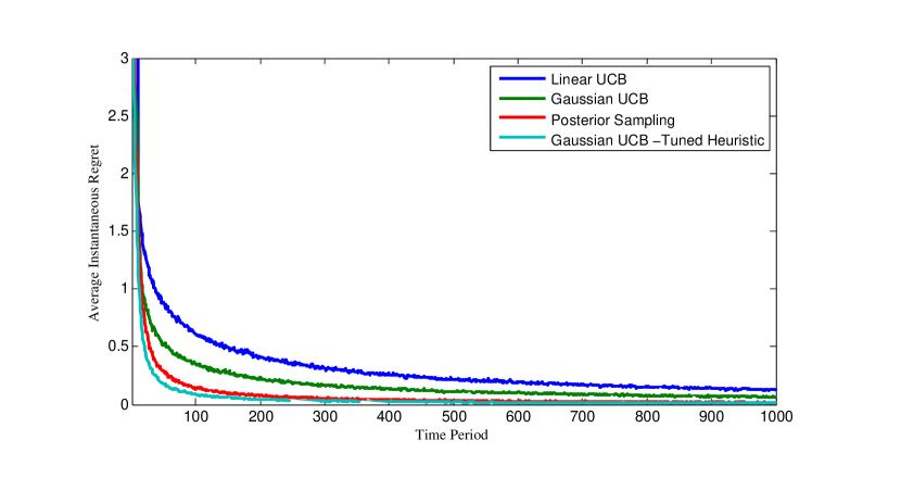
Figure 2: Portion of regret attributable to each time period.

Finally, it should be noted that the algorithms of [2, 35] have free parameters that must be chosen by the user. We have attempted to set these values in a way that minimizes average regret over the 1000 period time horizon. Both algorithms construct confidence bounds that hold with a pre-specified probability $1-\delta\in[0,1]$. Higher levels of $\delta$ lead to lower upper-confidence bounds, which we find improves performance. We set $\delta=1$ to minimize the average regret of the algorithms. The algorithm of [2] requires two other choices. We used a line search to set the algorithm’s regularization parameter to the level $\lambda=.025$, which minimizes cumulative regret. The algorithm of [2] also requires a uniform upper bound on $\left\|\theta\right\|$, but the Gaussian distribution is unbounded. We avoid this issue by providing the actual realized value $\left\|\theta\right\|$ as an input to algorithm.

9 Conclusion.

This paper has considered the use of a simple posterior sampling algorithm for learning to optimize actions when the decision maker is uncertain about how his actions influence performance. We believe that, particularly for difficult problem instances, this algorithm offers significant potential advantages because of its design simplicity and computational tractability. Despite its great potential, not much is known about posterior sampling when there are dependencies between actions. Our work has taken a significant step toward remedying this gap. We showed that the Bayesian regret of posterior sampling can be decomposed in terms of confidence sets, which allowed us to establish a number of new results on posterior sampling by leveraging prior work on UCB algorithms. We then used this regret decomposition to analyze posterior sampling in a very general framework, and developed Bayesian regret bounds that depend on a new notion of dimension.

In constructing these bounds, we have identified two factors that control the hardness of a particular multi-armed bandit problem. First, an agent’s ability to quickly attain near-optimal performance depends on the extent to which the reward value at one action can be inferred by sampling other actions. However, in order to select an action the agent must make inferences about many possible actions, and an error in its evaluation of any one could result in large regret. Our second measure of complexity controls for the difficulty of maintaining appropriate confidence sets simultaneously at every action. While our bounds are nearly tight in some cases, further analysis is likely to yield stronger results in other cases. We hope, however, that our work provides a conceptual foundation for the study of such problems, and inspires further investigation.

10 Details Regarding Lemma 6.3.

Lemma 6.3 follows as a special case of Theorem 1 of Abbasi-Yadkori et al. [2], which is much more general. Note that because reward noise $R_{t}-f_{\theta}(A_{t})$ is bounded in [-1,1], it is 1-subgaussian. Equation 12 in Abbasi-Yadkori et al. [2] gives a specialization of Theorem 1 to the problem we consider. It states that for any $\delta>0$, with probability at least $1-\delta$,

$$\left|\sum_{k=1}^{t}\left(\mathbf{1}_{\{A_{k}=a\}}(R_{k}-f_{\theta}(a)\right)\right|\leq\sqrt{\left(1+N_{t}(a)\right)\left(1+2\log\left(\frac{(1+N_{t}(a))^{1/2}}{\delta}\right)\right)}\,\,\,\,\,\,\,\forall t\in\mathbb{N}.$$

We choose $\delta=1/T$ and use that for $t\leq T$, $N_{t}(a)\leq T-1$ to show that with probability at least $1/T$,

$$\left|\sum_{k=1}^{t}\left(\mathbf{1}_{\{A_{k}=a\}}(R_{k}-f_{\theta}(a)\right)\right|\leq\sqrt{\left(1+N_{t}(a)\right)\left(1+3\log(T)\right)}\,\,\,\,\,\,\,\forall t\in\{1,..,T\}.$$

Since $1+N_{t}(a)\leq 2N_{t}(a)$ whenever $a$ has been played at least once, with probability at least $1/T$,

$$\left|\sum_{k=1}^{t}\left(\mathbf{1}_{\{A_{k}=a\}}(R_{k}-f_{\theta}(a)\right)\right|\leq\sqrt{\left(N_{t}(a)\right)\left(2+6\log(T)\right)}\,\,\,\,\,\,\,\forall t\in\{1,..,T\}.$$

11 Proof of Confidence bound.

11.1 Preliminaries: Martingale Exponential Inequalities.

Consider random variables $\left(Z_{n}|n\in\mathbb{N}\right)$ adapted to the filtration $\left(\mathcal{H}_{n}:\,n=0,1,...\right)$. Assume $\mathbb{E}\left[\exp\left\{\lambda Z_{i}\right\}\right]$ is finite for all $\lambda$. Define the conditional mean $\mu_{i}=\mathbb{E}\left[Z_{i}\mid\mathcal{H}_{i-1}\right]$. We define the conditional cumulant generating function of the centered random variable $\left[Z_{i}-\mu_{i}\right]$ by $\psi_{i}\left(\lambda\right)=\log\mathbb{E}\left[\exp\left(\lambda\left[Z_{i}-\mu_{i}\right]\right)\mid\mathcal{H}_{i-1}\right]$. Let

$$M_{n}(\lambda)=\exp\left\{\sum_{i=1}^{n}\lambda\left[Z_{i}-\mu_{i}\right]-\psi_{i}\left(\lambda\right)\right\}.$$

Lemma 11.1

$\left(M_{n}(\lambda)|n\in\mathbb{N}\right)$ is a Martinagale, and $\mathbb{E}M_{n}(\lambda)=1$.

Proof 11.2

Proof. By definition,

$$\mathbb{E}[M_{1}(\lambda)|\mathcal{H}_{0}]=\mathbb{E}[\exp\left\{\lambda\left[Z_{1}-\mu_{1}\right]-\psi_{1}\left(\lambda\right)\right\}|\mathcal{H}_{0}]=\mathbb{E}[\exp\left\{\lambda\left[Z_{1}-\mu_{1}\right]\right\}|\mathcal{H}_{0}]/\exp\left\{\psi_{1}\left(\lambda\right)\right\}=1.$$

Then, for any $n\geq 2$

$$\mathbb{E}\left[M_{n}(\lambda)\mid\mathcal{H}_{n-1}\right] = \mathbb{E}\left[\exp\left\{\sum_{i=1}^{n-1}\lambda\left[Z_{i}-\mu_{i}\right]-\psi_{i}\left(\lambda\right)\right\}\exp\left\{\lambda\left[Z_{n}-\mu_{n}\right]-\psi_{n}\left(\lambda\right)\right\}\mid\mathcal{H}_{n-1}\right]$$

$$= \exp\left\{\sum_{i=1}^{n-1}\lambda\left[Z_{i}-\mu_{i}\right]-\psi_{i}\left(\lambda\right)\right\}\mathbb{E}\left[\exp\left\{\lambda\left[Z_{n}-\mu_{n}\right]-\psi_{n}\left(\lambda\right)\right\}\mid\mathcal{H}_{n-1}\right]$$

$$= \exp\left\{\sum_{i=1}^{n-1}\lambda\left[Z_{i}-\mu_{i}\right]-\psi_{i}\left(\lambda\right)\right\}=M_{n-1}(\lambda).\Halmos$$

Lemma 11.3

For all $x\geq 0$ and $\lambda\geq 0$, $\mathbb{P}\left(\sum_{1}^{n}\lambda Z_{i}\leq x+\sum_{1}^{n}\left[\lambda\mu_{i}+\psi_{i}\left(\lambda\right)\right]\,\,\,\,\mbox{$\forall$}n\in\mathbb{N}\right)\geq 1-e^{-x}$.

Proof 11.4

Proof. For any $\lambda$, $M_{n}(\lambda)$ is a martingale with $\mathbb{E}M_{n}\left(\lambda\right)=1$. Therefore, for any stopping time $\tau$, $\mathbb{E}M_{\tau\wedge n}\left(\lambda\right)=1$. For arbitrary $x\geq 0$, define $\tau_{x}=\inf\left\{n\geq 0\mid M_{n}\left(\lambda\right)\geq x\right\}$ and note that $\tau_{x}$ is a stopping time corresponding to the first time $M_{n}$ crosses the boundary at $x$. Then, $\mathbb{E}M_{\tau_{x}\wedge n}(\lambda)=1$ and by Markov’s inequality:

$$x\mathbb{P}\left(M_{\tau_{x}\wedge n}\left(\lambda\right)\geq x\right)\leq\mathbb{E}M_{\tau_{x}\wedge n}(\lambda)=1.$$

We note that the event $\left\{M_{\tau_{x}\wedge n}\left(\lambda\right)\geq x\right\}=\bigcup_{k=1}^{n}\left\{M_{k}(\lambda)\geq x\right\}$. So we have shown that for all $x\geq 0$ and $n\geq 1$

$$\mathbb{P}\left(\bigcup_{k=1}^{n}\left\{M_{k}(\lambda)\geq x\right\}\right)\leq\frac{1}{x}.$$

Taking the limit as $n\rightarrow\infty$, and applying the monotone convergence theorem shows $\mathbb{P}\left(\bigcup_{k=1}^{\infty}\left\{M_{k}(\lambda)\geq x\right\}\right)\leq\frac{1}{x}$, Or, $\mathbb{P}\left(\bigcup_{k=1}^{\infty}\left\{M_{k}(\lambda)\geq e^{x}\right\}\right)\leq e^{-x}$. This then shows, using the definition of $M_{k}(\lambda)$, that

$$\mathbb{P}\left(\bigcup_{n=1}^{\infty}\left\{\sum_{i=1}^{n}\lambda\left[Z_{i}-\mu_{i}\right]-\psi_{i}\left(\lambda\right)\geq x\right\}\right)\leq e^{-x}.$$

11.2 Proof of Lemma 7.1.

XXXXX 1 (Lemma 7.1.)

$a=a$. For any $\delta>0$ and $f:\mathcal{A}\mapsto\mathbb{R}$, with probability at least $1-\delta$,

$$L_{2,t}(f)\geq L_{2,t}(f_{\theta})+\frac{1}{2}\left\|f-f_{\theta}\right\|_{2,E_{t}}^{2}-4\sigma^{2}\log\left(1/\delta\right)$$

simultaneously for all $t\in\mathbb{N}$.

We will transform our problem in order to apply the general exponential martingale result shown above. We set $\mathcal{H}_{t-1}$ to be the $\sigma$-algebra generated by $(H_{t},A_{t},\theta)$. By previous assumptions, $\epsilon_{t}:=R_{t}-f_{\theta}(A_{t})$ satisfies $\mathbb{E}[\epsilon_{t}|\mathcal{H}_{t-1}]=0$ and $\mathbb{E}\left[\exp\left\{\lambda\epsilon_{t}\right\}\mid{\mathcal{H}}_{t-1}\right]\leq\exp\left\{\frac{\lambda^{2}\sigma^{2}}{2}\right\}$ a.s. for all $\lambda$. Define $Z_{t}=\left(f_{\theta}\left(A_{t}\right)-R_{t}\right)^{2}-\left(f\left(A_{i}\right)-R_{t}\right)^{2}$

Proof 11.5

Proof. By definition $\sum_{1}^{T}Z_{t}=L_{2,T+1}(f_{\theta})-L_{2,T+1}(f)$. Some calculation shows that $Z_{t}=-\left(f(A_{t})-f_{\theta}(A_{t})\right)^{2}+2\left(f\left(A_{t}\right)-f_{\theta}\left(A_{t}\right)\right)\epsilon_{t}$. Therefore, the conditional mean and conditional cumulant generating function satisfy:

$$\mu_{t} = \mathbb{E}\left[Z_{t}\mid\mathcal{H}_{t-1}\right]=-\left(f\left(A_{t}\right)-f_{\theta}\left(A_{t}\right)\right)^{2}$$

$$\psi_{t}(\lambda) = \log\mathbb{E}\left[\exp\left(\lambda\left[Z_{t}-\mu_{t}\right]\right)\mid\mathcal{H}_{t-1}\right]$$

$$= \log\mathbb{E}\left[\exp\left(2\lambda\left(f\left(A_{t}\right)-f_{\theta}\left(A_{t}\right)\right)\epsilon_{t}\right)\mid\mathcal{H}_{t-1}\right]\leq\frac{(2\lambda\left[f\left(A_{t}\right)-f_{\theta}\left(A_{t}\right)\right])^{2}\sigma^{2}}{2}$$

Applying Lemma 11.3 shows that for all $x\geq 0$, $\lambda\geq 0$

$$\mathbb{P}\left(\sum_{k=1}^{t}\lambda Z_{k}\leq x-\lambda\sum_{k=1}^{t}\left(f\left(A_{k}\right)-f_{\theta}\left(A_{k}\right)\right)^{2}+\frac{\lambda^{2}}{2}\left(2f\left(A_{k}\right)-2f_{\theta}\left(A_{k}\right)\right)^{2}\sigma^{2}\,\,\,\,\mbox{$\forall$}t\in\mathbb{N}\right)\geq 1-e^{-x}.$$

Or, rearranging terms

$$\mathbb{P}\left(\sum_{k=1}^{t}Z_{k}\leq\frac{x}{\lambda}+\sum_{k=1}^{t}\left(f\left(A_{k}\right)-f_{\theta}\left(A_{k}\right)\right)^{2}\left(2\lambda\sigma^{2}-1\right)\,\,\,\,\mbox{$\forall$}t\in\mathbb{N}\right)\geq 1-e^{-x}.$$

Choosing $\lambda=\frac{1}{4\sigma^{2}}$, $x=\log\frac{1}{\delta}$, and using the definition of $\sum_{1}^{t}Z_{k}$ implies

$$\mathbb{P}\left(L_{2,t}(f)\geq L_{2,t}(f_{\theta})+\frac{1}{2}\left\|f-f_{\theta}\right\|_{2,E_{t}}^{2}-4\sigma^{2}\log\left(1/\delta\right)\,\,\,\,\mbox{$\forall$}t\in\mathbb{N}\right)\geq 1-\delta.$$

11.3 Least Squares Bound - Proof of Proposition 7.2.

XXXXX 2 (Proposition 7.2.)

For all $\delta>0$ and $\alpha>0$, if $\mathcal{F}_{t}=\left\{f\in\mathcal{F}:\,\left\|f-\hat{f}_{t}^{LS}\right\|_{2,E_{t}}\leq\sqrt{\beta^{*}_{t}\left(\mathcal{F},\delta,\alpha\right)}\right\}$ for all $t\in\mathbb{N}$, then

$$\mathbb{P}\left(f_{\theta}\in\bigcap_{t=1}^{\infty}\mathcal{F}_{t}\right)\geq 1-2\delta.$$

Proof 11.6

Proof. Let $\mathcal{F}^{\alpha}\subset\mathcal{F}$ be an $\alpha$–cover of $\mathcal{F}$ in the sup-norm in the sense that for any $f\in\mathcal{F}$ there is an $f^{\alpha}\in\mathcal{F}^{\alpha}$ such that $\left\|f^{\alpha}-f\right\|_{\infty}\leq\epsilon$. By a union bound, with probability at least $1-\delta$,

$$L_{2,t}(f^{\alpha})-L_{2,t}(f_{\theta})\geq\frac{1}{2}\left\|f^{\alpha}-f_{\theta}\right\|_{2,E_{t}}-4\sigma^{2}\log\left(\left|\mathcal{F}^{\alpha}\right|/\delta\right)\,\,\,\,\mbox{$\forall$}t\in\mathbb{N},\,f\in\mathcal{F}^{\alpha}.$$

Therefore, with probability at least $1-\delta$, for all $t\in\mathbb{N}$ and $f\in\mathcal{F}$:

$$L_{2,t}(f)-L_{2,t}(f_{\theta}) \geq \frac{1}{2}\left\|f-f_{\theta}\right\|_{2,E_{t}}^{2}-4\sigma^{2}\log\left(\left|\mathcal{F}^{\alpha}\right|/\delta\right)$$

$$+ \underbrace{\min_{f^{\alpha}\in\mathcal{F}^{\alpha}}\left\{\frac{1}{2}\left\|f^{\alpha}-f_{\theta}\right\|_{2,E_{t}}^{2}-\frac{1}{2}\left\|f-f_{\theta}\right\|_{2,E_{t}}^{2}+L_{2,t}(f)-L_{2,t}(f^{\alpha})\right\}}_{\text{Discretization\,\ Error}}.$$

Lemma 11.7, which we establish in the next section, asserts that with probability at least $1-\delta$ the discretization error is bounded for all $t$ by $\alpha\eta_{t}$ where $\eta_{t}:=t\left[8C+\sqrt{8\sigma^{2}\ln(4t^{2}/\delta)}\right]$. Since the least squares estimate $\hat{f}_{t}^{LS}$ has lower squared error than $f_{\theta}$ by definition, we find with probability at least $1-2\delta$

$$\frac{1}{2}\left\|\hat{f}_{t}^{\rm LS}-f_{\theta}\right\|_{2,E_{t}}^{2}\leq 4\sigma^{2}\log\left(\left|\mathcal{F}^{\alpha}\right|/\delta\right)+\alpha\eta_{t}.$$

Taking the infimum over the size of $\alpha$ covers implies:

$$\left\|\hat{f}_{t}^{LS}-f_{\theta}\right\|_{2,E_{t}}\leq\sqrt{8\sigma^{2}\log\left(N(\mathcal{F},\,\alpha,\,\left\|\cdot\right\|_{\infty})/\delta\right)+2\alpha\eta_{t}}\overset{{\rm def}}{=}\sqrt{\beta^{*}_{t}(\mathcal{F},\delta,\alpha)}.\Halmos$$

11.4 Discretization Error.

Lemma 11.7

If $f^{\alpha}$ satisfies $\left\|f-f^{\alpha}\right\|_{\infty}\leq\alpha$, then with probability at least $1-\delta$,

$$\left|\frac{1}{2}\left\|f^{\alpha}-f_{\theta}\right\|_{2,E_{t}}^{2}-\frac{1}{2}\left\|f-f_{\theta}\right\|_{2,E_{t}}^{2}+L_{2,t}(f)-L_{2,t}(f^{\alpha})\right|\leq\alpha t\left[8C+\sqrt{8\sigma^{2}\ln(4t^{2}/\delta)}\right]\,\,\ \forall t\in\mathbb{N}.$$ (9)

Proof 11.8

Proof. Since any two functions in $f,f^{\alpha}\in\mathcal{F}$ satisfy $\left\|f-f^{\alpha}\right\|_{\infty}\leq C$, it is enough to consider $\alpha\leq C$. We find

$$\left|\left(f^{\alpha}\right)^{2}(a)-\left(f\right)^{2}(a)\right|\leq\max_{-\alpha\leq y\leq\alpha}\left|\left(f(a)+y\right)^{2}-f(a)^{2}\right|=2f(a)\alpha+\alpha^{2}\leq 2C\alpha+\alpha^{2}$$

which implies

$$\left|\left(f^{\alpha}(a)-f_{\theta}(a)\right)^{2}-\left(f(a)-f_{\theta}(a)\right)^{2}\right| = \left|\left[\left(f^{\alpha}\right)(a)^{2}-f(a)^{2}\right]+2f_{\theta}(a)\left(f(a)-f^{\alpha}(a)\right)\right|\leq 4C\alpha+\alpha^{2}$$

$$\left|\left(R_{t}-f(a)\right)^{2}-\left(R_{t}-f^{\alpha}(a)\right)^{2}\right| = \left|2R_{t}\left(f^{\alpha}(a)-f(a)\right)+f(a)^{2}-f^{\alpha}(a)^{2}\right|\leq 2\alpha\left|R_{t}\right|+2C\alpha+\alpha^{2}$$

Summing over $t$, we find that the left hand side of (9) is bounded by

$$\sum_{k=1}^{t-1}\left(\frac{1}{2}\left[4C\alpha+\alpha^{2}\right]+\left[2\alpha\left|R_{k}\right|+2C\alpha+\alpha^{2}\right]\right)\leq\alpha\sum_{k=1}^{t-1}\left(6C+2\left|R_{k}\right|\right).$$

Because $\epsilon_{k}$ is sub-Gaussian, $\mathbb{P}\left(\left|\epsilon_{k}\right|>\sqrt{2\sigma^{2}\ln(2/\delta)}\right)\leq\delta$. By a union bound,

$$\mathbb{P}\left(\exists k\,s.t.\,\,\left|\epsilon_{k}\right|>\sqrt{2\sigma^{2}\ln(4t^{2}/\delta)}\right)\leq\frac{\delta}{2}\sum_{1}^{\infty}\frac{1}{k^{2}}\leq\delta.$$

Since $\left|R_{k}\right|\leq C+\left|\epsilon_{k}\right|$ this shows that with probability at least $1-\delta$ the discretization error is bounded for all $t$ by $\alpha\eta_{t}$ where $\eta_{t}:=t\left[8C+2\sqrt{2\sigma^{2}\ln(4t^{2}/\delta)}\right]$.

12 Bounds on Eluder Dimension for Common Function Classes.

Definition 7.11, which defines the eluder dimension of a class of functions, can be equivalently written as follows. The $\epsilon$-eluder dimension of a class of functions $\mathcal{F}$ is the length of the longest sequence $a_{1},..,a_{\tau}$ such that for some $\epsilon^{\prime}\geq\epsilon$

$$w_{k}:=\sup\left\{\left(f_{\rho_{1}}-f_{\rho_{1}}\right)(a_{k}):\sqrt{\sum_{i=1}^{k-1}\left(f_{\rho_{1}}-f_{\rho_{2}}\right)^{2}\left(a_{i}\right)}\leq\epsilon^{\prime}\,\,\rho_{1},\rho_{2}\in\Theta\right\}>\epsilon^{\prime}$$ (10)

for each $k\leq\tau$.

12.1 Finite Action Spaces.

Any action is $\epsilon^{\prime}$–dependent on itself since

$$\sup\left\{\left(f_{\rho_{1}}-f_{\rho_{1}}\right)(a):\sqrt{\left(f_{\rho_{1}}-f_{\rho_{2}}\right)^{2}\left(a\right)}\leq\epsilon^{\prime}\,\,\rho_{1},\rho_{2}\in\Theta\right\}\leq\epsilon^{\prime}.$$

Therefore, for all $\epsilon>0$, the $\epsilon$-eluder dimension of $\mathcal{A}$ is bounded by $|\mathcal{A}|$.

12.2 Linear Case.

Proposition 12.1

Suppose $\Theta\subset\mathbb{R}^{d}$ and $f_{\theta}(a)=\theta^{T}\phi(a)$. Assume there exist constants $\gamma$, and $S$, such that for all $a\in\mathcal{A}$ and $\rho\in\Theta$, $\left\|\rho\right\|_{2}\leq S$, and $\left\|\phi(a)\right\|_{2}\leq\gamma$. Then ${\rm dim}_{E}(\mathcal{F},\epsilon)\leq 3d\frac{e}{e-1}\ln\left\{3+3\left(\frac{2S}{\epsilon}\right)^{2}\right\}+1$.

To simplify the notation, define $w_{k}$ as in (10), $\phi_{k}=\phi\left(a_{k}\right)$, $\rho=\rho_{1}-\rho_{2}$, and $\Phi_{k}=\sum_{i=1}^{k-1}\phi_{i}\phi_{i}^{T}$. In this case, $\sum_{i=1}^{k-1}\left(f_{\rho_{1}}-f_{\rho_{2}}\right)^{2}\left(a_{i}\right)=\rho^{T}\Phi_{k}\rho$, and by the triangle inequality $\left\|\rho\right\|_{2}\leq 2S$. The proof follows by bounding the number of times $w_{k}>\epsilon^{\prime}$ can occur.

Step 1: If $w_{k}\geq\epsilon^{\prime}$ then $\phi_{k}^{T}V_{k}^{-1}\phi_{k}\geq\frac{1}{2}$ where $V_{k}:=\Phi_{k}+\lambda I$ and $\lambda=\left(\frac{\epsilon^{\prime}}{2S}\right)^{2}$.

Proof 12.2

Proof. We find $w_{k}\leq\max\left\{\rho^{T}\phi_{k}:\,\rho^{T}\Phi_{k}\rho\leq(\epsilon^{\prime})^{2},\,\,\rho^{T}I\rho\leq(2S)^{2}\right\}\leq\max\left\{\rho^{T}\phi_{k}:\,\rho^{T}V_{k}\rho_{k}\leq 2(\epsilon^{\prime})^{2}\right\}=\sqrt{2(\epsilon^{\prime})^{2}}\left\|\phi_{k}\right\|_{V_{k}^{-1}}$. The second inequality follows because any $\rho$ that is feasible for the first maximization problem must satisfy $\rho^{T}V_{k}\rho\leq(\epsilon^{\prime})^{2}+\lambda(2S)^{2}=2(\epsilon^{\prime})^{2}$. By this result, $w_{k}\geq\epsilon^{\prime}$ implies $\left\|\phi_{k}\right\|_{V_{k}^{-1}}^{2}\geq 1/2$.

Step 2: If $w_{i}\geq\epsilon^{\prime}$ for each $i<k$ then $\det V_{k}\geq\lambda^{d}\left(\frac{3}{2}\right)^{k-1}$ and $\det V_{k}\leq\left(\frac{\gamma^{2}\left(k-1\right)}{d}+\lambda\right)^{d}$.

Proof 12.3

Proof. Since $V_{k}=V_{k-1}+\phi_{k}\phi_{k}^{T}$, using the Matrix Determinant Lemma,

$$\det V_{k}=\det V_{k-1}\left(1+\phi_{t}^{T}V_{k}^{-1}\phi_{t}\right)\geq\det V_{k-1}\left(\frac{3}{2}\right)\geq...\geq\det\left[\lambda I\right]\left(\frac{3}{2}\right)^{k-1}=\lambda^{d}\left(\frac{3}{2}\right)^{k-1}.$$

Recall that $\det V_{k}$ is the product of the eigenvalues of $V_{k}$, whereas $\text{trace}\left[V_{k}\right]$ is the sum. As noted in [17], $\det V_{k}$ is maximized when all eigenvalues are equal. This implies: $\det V_{k}\leq\left(\frac{\text{trace}\left[V_{k}\right]}{d}\right)^{d}\leq\left(\frac{\gamma^{2}\left(t-1\right)}{d}+\lambda\right)^{d}$.

Step 3: Complete Proof.

Proof 12.4

Proof. Manipulating the result of Step 2 shows $k$ must satisfy the inequality: $\left(\frac{3}{2}\right)^{\frac{k-1}{d}}\leq\alpha_{0}\left[\frac{k-1}{d}\right]+1$ where $\alpha_{0}=\left(\frac{\gamma^{2}}{\lambda}\right)=\left(\frac{2S\gamma}{\epsilon^{\prime}}\right)^{2}$. Let $B(x,\alpha)=\max\left\{B:\,\left(1+x\right)^{B}\leq\alpha B+1\right\}$. The number of times $w_{k}>\epsilon^{\prime}$ can occur is bounded by $dB(1/2,\alpha_{0})+1$.

We now derive an explicit bound on $B(x,\alpha)$ for any $x\leq 1$. Note that any $B\geq 1$ must satisfy the inequality: $\ln\left\{1+x\right\}B\leq\ln\left\{1+\alpha\right\}+\ln B$. Since $\ln\left\{1+x\right\}\geq x/(1+x)$, using the transformation of variables $y=B\left[x/(1+x)\right]$ gives:

$$y\leq\ln\left\{1+\alpha\right\}+\ln\frac{1+x}{x}+\ln y\leq\ln\left\{1+\alpha\right\}+\ln\frac{1+x}{x}+\frac{y}{e}\implies y\leq\frac{e}{e-1}\left(\ln\left\{1+\alpha\right\}+\ln\frac{1+x}{x}\right).$$

This implies $B(x,\alpha)\leq\frac{1+x}{x}\frac{e}{e-1}\left(\ln\left\{1+\alpha\right\}+\ln\frac{1+x}{x}\right)$. The claim follows by plugging in $\alpha=\alpha_{0}$ and $x=1/2$.

12.3 Generalized Linear Models.

Proposition 12.5

Suppose $\Theta\subset\mathbb{R}^{d}$ and $f_{\theta}(a)=g(\theta^{T}\phi(a))$ where $g(\cdot)$ is a differentiable and strictly increasing function. Assume there exist constants $\underline{h}$, $\overline{h}$, $\gamma$, and $S$, such that for all $a\in\mathcal{A}$ and $\rho\in\Theta$, $0<\underline{h}\leq g^{\prime}(\rho^{T}\phi(a))\leq\overline{h}$, $\left\|\rho\right\|_{2}\leq S$, and $\left\|\phi(a)\right\|_{2}\leq\gamma$. Then ${\rm dim}_{E}(\mathcal{F},\epsilon)\leq 3dr^{2}\frac{e}{e-1}\ln\left\{3r^{2}+3r^{2}\left(\frac{2S\overline{h}}{\epsilon}\right)^{2}\right\}+1$.

The proof follows three steps which closely mirror those used to prove Proposition 12.1.

Step 1: If $w_{k}\geq\epsilon^{\prime}$ then $\phi_{k}^{T}V_{k}^{-1}\phi_{k}\geq\frac{1}{2r^{2}}$ where $V_{k}:=\Phi_{k}+\lambda I$ and $\lambda=\left(\frac{\epsilon^{\prime}}{2S\underline{h}}\right)^{2}$.

Proof 12.6

Proof. By definition $w_{k}\leq\max\left\{g\left(\rho^{T}\phi_{k}\right):\,\sum_{i=1}^{k-1}g\left(\rho^{T}\phi(a_{i})\right)^{2}\leq(\epsilon^{\prime})^{2},\,\,\rho^{T}I\rho\leq(2S)^{2}\right\}$. By the uniform bound on $g^{\prime}(\cdot)$ this is less than $\max\left\{\overline{h}\rho^{T}\phi_{k}:\,\underline{h}^{2}\rho^{T}\Phi_{k}\rho\leq(\epsilon^{\prime})^{2},\rho^{T}I\rho\leq(2S)^{2}\right\}\leq\max\left\{\overline{h}\rho^{T}\phi_{k}:\,\underline{h}^{2}\rho^{T}V_{k}\rho\leq 2(\epsilon^{\prime})^{2}\right\}=\sqrt{2(\epsilon^{\prime})^{2}/r^{2}}\left\|\phi_{k}\right\|_{V_{k}^{-1}}$.

Step 2: If $w_{i}\geq\epsilon^{\prime}$ for each $i<k$ then $\det V_{k}\geq\lambda^{d}\left(\frac{3}{2}\right)^{k-1}$ and $\det V_{k}\leq\left(\frac{\gamma^{2}\left(k-1\right)}{d}+\lambda\right)^{d}$.

Step 3: Complete Proof.

Proof 12.7

Proof. The above inequalities imply $k$ must satisfy: $\left(1+\frac{1}{2r^{2}}\right)^{\frac{k-1}{d}}\leq\alpha_{0}\left[\frac{k-1}{d}\right]$ where $\alpha_{0}=\gamma^{2}/\lambda$. Therefore, as in the linear case, the number of times $w_{k}>\epsilon^{\prime}$ can occur is bounded by $dB(\frac{1}{2r^{2}},\alpha_{0})+1$. Plugging these constants into the earlier bound $B(x,\alpha)\leq\frac{1+x}{x}\frac{e}{e-1}\left(\ln\left\{1+\alpha\right\}+\ln\frac{1+x}{x}\right)$ and using $1+x\leq 3/2$ yields the result.

Daniel Russo is supported by a Burt and Deedee McMurty Stanford Graduate Fellowship. This work was supported in part by Award CMMI-0968707 from the National Science Foundation.

References

- Abbasi-Yadkori et al. [2009] Abbasi-Yadkori, Y., A. Antos, C. Szepesvári. 2009. Forced-exploration based algorithms for playing in stochastic linear bandits. COLT Workshop on On-line Learning with Limited Feedback.
- Abbasi-Yadkori et al. [2011] Abbasi-Yadkori, Y., D. Pál, C. Szepesvári. 2011. Improved algorithms for linear stochastic bandits. Advances in Neural Information Processing Systems 24.
- Abbasi-Yadkori et al. [2012] Abbasi-Yadkori, Y., D. Pal, C. Szepesvári. 2012. Online-to-confidence-set conversions and application to sparse stochastic bandits. Conference on Artificial Intelligence and Statistics (AISTATS).
- Agrawal and Goyal [2012a] Agrawal, S., N. Goyal. 2012a. Analysis of Thompson sampling for the multi-armed bandit problem.
- Agrawal and Goyal [2012b] Agrawal, S., N. Goyal. 2012b. Further optimal regret bounds for Thompson sampling. arXiv preprint arXiv:1209.3353 .
- Agrawal and Goyal [2012c] Agrawal, S., N. Goyal. 2012c. Thompson sampling for contextual bandits with linear payoffs. arXiv preprint arXiv:1209.3352 .
- Amin et al. [2011] Amin, K., M. Kearns, U. Syed. 2011. Bandits, query learning, and the haystack dimension. Proceedings of the 24th Annual Conference on Learning Theory (COLT).
- Audibert and Bubeck [2009] Audibert, J.-Y., S. Bubeck. 2009. Minimax policies for bandits games. COLT 2009 .
- Auer et al. [2002] Auer, P., N. Cesa-Bianchi, P. Fischer. 2002. Finite-time analysis of the multiarmed bandit problem. Machine learning 47(2) 235–256.
- Beygelzimer et al. [2011] Beygelzimer, A., J. Langford, L. Li, L. Reyzin, R.E. Schapire. 2011. Contextual bandit algorithms with supervised learning guarantees. Conference on Artificial Intelligence and Statistics (AISTATS), vol. 15. JMLR Workshop and Conference Proceedings.
- Bubeck and Cesa-Bianchi [2012] Bubeck, S., N. Cesa-Bianchi. 2012. Regret analysis of stochastic and nonstochastic multi-armed bandit problems. arXiv preprint arXiv:1204.5721 .
- Bubeck and Liu [2013] Bubeck, S., C.-Y. Liu. 2013. Prior-free and prior-dependent regret bounds for thompson sampling. Advances in Neural Information Processing Systems.
- Bubeck et al. [2011] Bubeck, S., R. Munos, G. Stoltz, Cs. Szepesvári. 2011. X-armed bandits. Journal of Machine Learning Research 12 1655–1695. Submitted on 21/1/2010.
- Cappé et al. [2013] Cappé, O., A. Garivier, O.-A. Maillard, R. Munos, G. Stoltz. 2013. Kullback-Leibler upper confidence bounds for optimal sequential allocation. Annals of Statistics 41(3) 1516–1541.
- Chapelle and Li [2011] Chapelle, O., L. Li. 2011. An empirical evaluation of Thompson sampling. Neural Information Processing Systems (NIPS).
- D. and Montanari [2012] D., Yash, A. Montanari. 2012. Linear bandits in high dimension and recommendation systems. Communication, Control, and Computing (Allerton), 2012 50th Annual Allerton Conference on. IEEE, 1750–1754.
- Dani et al. [2008] Dani, V., T.P. Hayes, S.M. Kakade. 2008. Stochastic linear optimization under bandit feedback. Proceedings of the 21st Annual Conference on Learning Theory (COLT). 355–366.
- Filippi et al. [2010] Filippi, S., O. Cappé, A. Garivier, C. Szepesvári. 2010. Parametric bandits: The generalized linear case. Advances in Neural Information Processing Systems 23 1–9.
- Gittins et al. [2011] Gittins, J., K. Glazebrook, R. Weber. 2011. Multi-Armed Bandit Allocation Indices. John Wiley & Sons, Ltd.
- Gittins and Jones [1979] Gittins, J.C., D.M. Jones. 1979. A dynamic allocation index for the discounted multiarmed bandit problem. Biometrika 66(3) 561–565.
- Gopalan et al. [2013] Gopalan, A., S. Mannor, Y. Mansour. 2013. Thompson sampling for complex bandit problems. arXiv preprint arXiv:1311.0466 .
- Kauffmann et al. [2012] Kauffmann, E., N. Korda, R. Munos. 2012. Thompson sampling: an asymptotically optimal finite time analysis. International Conference on Algorithmic Learning Theory.
- Kleinberg et al. [2008] Kleinberg, R., A. Slivkins, E. Upfal. 2008. Multi-armed bandits in metric spaces. Proceedings of the 40th ACM Symposium on Theory of Computing.
- Korda et al. [2013] Korda, N., E. Kaufmann, R. Munos. 2013. Thompson sampling for one-dimensional exponential family bandits. Advances in Neural Information Processing Systems.
- Lai [1987] Lai, T.L. 1987. Adaptive treatment allocation and the multi-armed bandit problem. The Annals of Statistics 1091–1114.
- Lai and Robbins [1985] Lai, T.L., H. Robbins. 1985. Asymptotically efficient adaptive allocation rules. Advances in applied mathematics 6(1) 4–22.
- Lehmann and Casella [1998] Lehmann, E.L., G. Casella. 1998. Theory of point estimation, vol. 31. Springer.
- Li and Chapelle [2012] Li, L., O. Chapelle. 2012. Open problem: Regret bounds for Thompson sampling. Proceedings of the 25th Annual Conference on Learning Theory (COLT).
- Li [2013] Li, Lihong. 2013. Generalized thompson sampling for contextual bandits. arXiv preprint arXiv:1310.7163 .
- May et al. [2012] May, B.C., N. Korda, A. Lee, D.S. Leslie. 2012. Optimistic Bayesian sampling in contextual-bandit problems. The Journal of Machine Learning Research 98888 2069–2106.
- Rusmevichientong and Tsitsiklis [2010] Rusmevichientong, P., J.N. Tsitsiklis. 2010. Linearly parameterized bandits. Mathematics of Operations Research 35(2) 395–411.
- Ryzhov et al. [2012] Ryzhov, I.O., W.B. Powell, P.I. Frazier. 2012. The knowledge gradient algorithm for a general class of online learning problems. Operations Research 60(1) 180–195.
- Sahni [1974] Sahni, A. 1974. Computationally related problems. SIAM Journal on Computing 3(4) 262–279.
- Scott [2010] Scott, S.L. 2010. A modern Bayesian look at the multi-armed bandit. Applied Stochastic Models in Business and Industry 26(6) 639–658.
- Srinivas et al. [2012] Srinivas, N., A. Krause, S.M. Kakade, M. Seeger. 2012. Information-theoretic regret bounds for Gaussian process optimization in the bandit setting. Information Theory, IEEE Transactions on 58(5) 3250 –3265. 10.1109/TIT.2011.2182033.
- Valko et al. [2013] Valko, M., A. Carpentier, R. Munos. 2013. Stochastic simultaneous optimistic optimization. Sanjoy Dasgupta, David Mcallester, eds., Proceedings of the 30th International Conference on Machine Learning (ICML-13), vol. 28. JMLR Workshop and Conference Proceedings, 19–27.