The Hele-Shaw asymptotics for mechanical
models of tumor growth

Abstract

Models of tumor growth, now commonly used, present several levels of complexity, both in terms of the biomedical ingredients and the mathematical description. The simplest ones contain competition for space using purely fluid mechanical concepts. Another possible ingredient is the supply of nutrients through vasculature. The models can describe the tissue either at the level of cell densities, or at the scale of the solid tumor, in this latter case by means of a free boundary problem.

Our first goal here is to formulate a free boundary model of Hele-Shaw type, a variant including growth terms, starting from the description at the cell level and passing to a certain limit. A detailed mathematical analysis of this purely mechanical model is performed. Indeed, we are able to prove strong convergence in passing to the limit, with various uniform gradient estimates; we also prove uniqueness for the asymptotic Hele-Shaw type problem. The main tools are nonlinear regularizing effects for certain porous medium type equations, regularization techniques à la Steklov, and a Hilbert duality method for uniqueness. At variance with the classical Hele-Shaw problem, here the geometric motion governed by the pressure is not sufficient to completely describe the dynamics. A complete description requires the equation on the cell number density.

Using this theory as a basis, we go on to consider the more complex model including nutrients. We obtain the equation for the limit of the coupled system; the method relies on some BV bounds and space/time a priori estimates. Here, new technical difficulties appear, and they reduce the generality of the results in terms of the initial data. Finally, we prove uniqueness for the system, a main mathematical difficulty.

Key words Tumor growth; Hele-Shaw equation; free boundary problems; porous media; Hilbert uniqueness method.

Mathematics Subject Classification 35K55; 35B25; 76D27; 92C50.

1 Motivation and tumor growth models

In the understanding of cancer development, mathematical modeling and numerical simulations have nowadays complemented experimental and clinical observations. The field is now mature; books and surveys are available, as for example [3, 4, 24, 36]. A first class of models, initiated in the 70’s by Greenspan [31], has considered that cancerous cells multiplication is limited by nutrients (glucosis, oxygen) brought by blood vessels. Models of this class rely on two kinds of descriptions; either they describe the dynamics of cell population density [12] or they consider the ‘geometric’ motion of the tumor through a free boundary problem; see [18, 19, 26] and the references therein. This stage lasts until the tumor reaches the size of $\approx 1$mm; then lack of nutrients leads to cell necrosis which triggers neovasculatures development [15] that supply the tumor with enough nourishment. This has motivated a new generation of models where growth is limited by the competition for space [11], turning the modeling effort towards mechanical concepts, considering tissues as multiphasic fluids (the phases could be intersticial water, healthy and tumor cells, extra-cellular matrix …) [13, 14, 37]. This point of view is now sustained by experimental evidence [38]. The term ‘homeostatic pressure’, coined recently, denotes the lower pressure that prevents cell multiplication by contact inhibition.

The aim of this paper is to explain how asymptotic analysis can link the two main approaches, cell density models and free boundary models, in the context of fluid mechanics. We depart from the simplest cell population density model, proposed in [13], in which the cell population density $\varrho(x,t)$ evolves under pressure forces and cell multiplication according to the equation

(1.1) $$\partial_{t}\varrho-{\rm div}(\varrho\nabla p)=\varrho\;\Phi(p),$$

where $p$ is the pressure field. Pressure-limited growth is described by the term $\Phi(p)$, which typically satisfies

(1.2) $$\Phi^{\prime}(p)<0\qquad\text{and}\qquad\Phi(p_{M})=0$$

for some $p_{M}>0$ (the homeostatic pressure). The pressure is assumed to be a given increasing function of the density. A representative example is

(1.3) $$p=P_{m}(\varrho):=\frac{m}{m-1}\left(\frac{\varrho}{\varrho_{c}}\right)^{m-1}$$

with parameter $m>1$. In the free boundary problem to be discussed later, the value $\varrho_{c}$ represents the maximum packing density of cells, as discussed in [41].

Nutrients consumed by the tumor cells and brought by the capillary blood network are a usual additional ingredient to the modeling. The situation is described in that case by the system

(1.4) $$\begin{cases}\displaystyle\partial_{t}\varrho-{\rm div}(\varrho\nabla p)=\varrho\;\Phi(p,c),\\[5.69054pt] \displaystyle\partial_{t}c-\Delta c=-\varrho\;\Psi(p,c),\\[5.69054pt] c(x,t)=c_{B}>0\qquad\text{as }\;|x|\to\infty,\end{cases}$$

where $c$ denotes the density of nutrients, and $c_{B}$ the far field supply of nutrients (from blood vessels). The coupling functions $\Phi$, $\Psi$ are assumed to be smooth and to satisfy the natural hypotheses

(1.5) $$\begin{array}[]{lll}\displaystyle\partial_{p}\Phi<0,&\displaystyle\partial_{c}\Phi\geq 0,&\displaystyle\Phi(p_{M},c_{B})=0,\\[10.0pt] \displaystyle\partial_{p}\Psi\leq 0,&\displaystyle\partial_{c}\Psi\geq 0,&\displaystyle\Psi(p,0)=0.\end{array}$$

Variants are possible; for instance, we could assume that nutrients are released continuously from a vasculature, then leading to an equation as

$$\partial_{t}c-\Delta c=-\varrho\;\Psi(p,c)+r(c_{B}-c).$$

We will consider below the purely mechanical model (1.1) under assumptions (1.2)–(1.3), and also the system (1.4), where nutrients are taken into account, under assumptions (1.3) and (1.5). In both cases we will show that the asymptotic limit $m\to\infty$ yields a free boundary model of Hele-Shaw type, as we were looking for.

Let us recall that the mathematical theory of the limit for an equation like (1.1) in the absence of a growth term is well developed, the asymptotic limit being in this case the standard Hele-Shaw model for incompressible fluids with free boundaries. Early papers on the subject [5, 6, 8, 9, 22, 25, 27, 39] consider situations in which mass is conserved and the limit is stationary. In order to have a non-trivial limit evolution one needs some source, either in the equation or at the boundary of the domain. A first example, in which there is an inwards flux at infinity, is given in [2], where the authors study the limit $m\to\infty$ of self-similar focusing (hole-filling) solutions to the porous medium equation $u_{t}=\Delta u^{m}$. A second example, in which there is a bounded boundary with a nontrivial boundary data, was first considered in [28], and later on in [29, 32, 34, 35]. To our knowledge, the present paper is the first one in which the evolution in the limit is produced by a nonlinear source term in the equation. In order to pass to the limit, three approaches have been used: weak solutions, variational formulations (using the so-called Baiocchi variable), and viscosity solutions; see [33, 34] for this last case. The weak formulation of Hele-Shaw was first introduced in [20], and the variational formulation in [23].

Let us also mention that the Hele-Shaw graph, and hence the Hele-Shaw equation, can be approximated in other ways, for example by the Stefan problem. This situation has also been considered in the literature, even in situations where there is an evolution in the limit; see for instance [10, 30, 34].

We would like to stress that including the growth term is not a simple change: several powerful but specific tools do not apply any longer. More deeply, as we explain later, several approaches have no chance to work as they are. This is the reason why we will work on an equation for the cell density itself rather than the pressure. We also would like to point out that models of Hele-Shaw type are still an active field arising in several unexpected applications, see for instance [21], and that surface tension is not covered by the present work; see [16, 18, 19, 26].

Organization of the paper. We first study the simplest mechanical model in Section 2. The more complex model with nutrients is studied in Section 4. The uniqueness proofs for both cases are highly technical, and are performed separately, in sections 3 and 5. These two sections can safely be skipped by the readers who are mainly interested in the applications. We finally include an appendix devoted to some interesting examples for the purely mechanical model, that illustrate several phenomena.

Some notations. We will use several times the abridged notations $\varrho(t)$, $p(t)$, meaning $\varrho(t)(x)=\varrho(x,t)$, $p(t)(x)=p(x,t)$. Given any $T>0$, we denote $Q_{T}=\mathbb{R}^{N}\times(0,T)$, while $Q=\mathbb{R}^{N}\times(0,\infty)$.

2 Purely fluid mechanical model

We start our analysis by a detailed investigation of the purely mechanical model (1.1), which does not take into account the consumption of nutrients, with a pressure field given by (1.3). A simple change of scale allows us to assume without loss of generality that $\varrho_{c}=1$. We arrive to the porous medium type equation, set on $Q$,

(2.1) $$\partial_{t}\varrho=\Delta\varrho^{m}+\varrho\Phi(p),\qquad p=P_{m}(\varrho):=\frac{m}{m-1}\varrho^{m-1},\qquad\varrho(0)=\varrho_{m}^{0}.$$

We assume that the initial data $\varrho_{m}^{0}$ are such that, for some $\varrho^{0}\in L^{1}_{+}(\mathbb{R}^{N})$,

(2.2) $$\left\{\begin{array}[]{ll}\varrho_{m}^{0}\geq 0,&P_{m}(\varrho_{m}^{0})\leq p_{M},\\[10.0pt] \|\varrho_{m}^{0}-\varrho^{0}\|_{L^{1}(\mathbb{R}^{N})}\underset{m\to\infty}{\longrightarrow}0,&\|\partial_{x_{i}}\varrho^{0}_{m}\|_{L^{1}(\mathbb{R}^{N})}\leq C,\quad i=1,\dots,N.\end{array}\right.$$

2.1 Main results

Free boundary limit. Let $(\varrho_{m},p_{m})$ be the unique bounded weak solution to (2.1). We will prove that, along some subsequence, there is a limit as $m\to\infty$ which turns out to be a solution to a free boundary problem of Hele-Shaw type.

Theorem 2.1

Let $\Phi$ and $\{\varrho_{m}^{0}\}$ satisfy (1.2) and (2.2) respectively. Then, after extraction of subsequences, both the density $\varrho_{m}$ and the pressure $p_{m}$ converge for all $T>0$ strongly in $L^{1}(Q_{T})$ as $m\to\infty$ to limits $\varrho_{\infty}\in C\big{(}[0,\infty);L^{1}(\mathbb{R}^{N})\big{)}\cap BV(Q_{T})$, $p_{\infty}\in BV(Q_{T})$, that satisfy $0\leq\varrho_{\infty}\leq 1$, $0\leq p_{\infty}\leq p_{M}$, and

(2.3) $$\partial_{t}\varrho_{\infty}=\Delta p_{\infty}+\varrho_{\infty}\Phi(p_{\infty})\quad\text{in }\mathcal{D}^{\prime}(Q),\qquad\varrho_{\infty}(0)=\varrho^{0}\quad\text{in }L^{1}(\mathbb{R}^{N}),$$

plus the relation $p_{\infty}\in P_{\infty}(\varrho_{\infty})$, where $P_{\infty}$ is the Hele-Shaw monotone graph

(2.4) $$P_{\infty}(\varrho)=\left\{\begin{array}[]{ll}0,&0\leq\varrho<1,\\[3.0pt] [0,\infty),&\varrho=1.\end{array}\right.$$

Note that (2.4) means that a.e. $P_{\infty}\geq 0$ and $P_{\infty}=0$ a.e. in $\{0\leq\varrho<1\}$.

We will obtain also several important qualitative properties for the limit. On the one hand, the ‘tumor is growing’ and the pressure increases, that is,

(2.5) $$\partial_{t}\varrho_{\infty}\geq 0,\qquad\partial_{t}p_{\infty}\geq 0\qquad\text{in }\mathcal{D}^{\prime}(Q).$$

On the other hand, if the initial data $\{\varrho_{m}^{0}\}$ have a common compact support, then the limit solution propagates with a finite speed: $\varrho_{\infty}(t)$ and $p_{\infty}(t)$ are compactly supported for all $t>0$. Finally, the constructed limit solution enjoys the monotonicity property, inherited from the case where $m$ is finite,

$$\varrho^{0}\geq\bar{\varrho}^{0}\;\Longrightarrow\;\left\{\begin{array}[]{l}\varrho_{\infty}(t)\geq\bar{\varrho}_{\infty}(t),\\[8.0pt] p_{\infty}(t)\geq\bar{p}_{\infty}(t).\end{array}\right.$$

Transport equation and complementarity formula. We will also obtain $L^{2}$ estimates on the gradients $\nabla p_{m}$ that will show on the one hand that

$$\nabla p_{\infty}\in L^{2}(Q_{T})\quad\text{for all }T>0,$$

and on the other hand that $(\varrho_{\infty},p_{\infty})$ solves a transport equation.

Theorem 2.2

The limit solution $(\varrho_{\infty},p_{\infty})$ obtained in Theorem 2.1 satisfies

$$\partial_{t}\varrho_{\infty}-{\rm div}\left(\varrho_{\infty}\nabla p_{\infty}\right)=\varrho_{\infty}\Phi(p_{\infty})$$

in a weak sense.

A direct calculation shows that the pressure $p_{m}$ satisfies

(2.6) $$\partial_{t}p_{m}=(m-1)p_{m}\Delta p_{m}+|\nabla p_{m}|^{2}+(m-1)p_{m}\Phi(p_{m}).$$

Hence, if we let $m\to\infty$, we formally obtain the complementarity formula

(2.7) $$p_{\infty}\big{(}\Delta p_{\infty}+\Phi(p_{\infty})\big{)}=0.$$

This formal computation can be made rigorous.

Theorem 2.3

Under the assumptions of Theorem 2.1, the limit pressure $p_{\infty}$ satisfies the complementarity formula

(2.8) $$\int_{\mathbb{R}^{N}}\left(-|\nabla p_{\infty}|^{2}+p_{\infty}\Phi(p_{\infty})\right)=0\quad\text{for almost every }t>0.$$

It is worth noticing that (2.8) is equivalent to the strong convergence of $\nabla p_{m}$ in $L^{2}(Q_{T})$ for all $T>0$; see Lemma 2.5.

Since the limit pressure $p_{\infty}$ is expected to be continuous in space for all positive times, the positivity set

$$\Omega(t):=\{x;\;p_{\infty}(x,t)>0\},$$

should be well defined for all $t>0$. Notice that it coincides almost everywhere with the set where $\varrho_{\infty}=1$; see Figure 1. Indeed, on the one hand, by the definition of the graph $P_{\infty}$ we have $\Omega(t)\subset\{x;\;\varrho_{\infty}(x,t)=1\}$; on the other hand, if we had $p_{\infty}=0$ and $\varrho_{\infty}=1$ in some set with positive measure, then $\varrho_{\infty}$ would continue to grow (exponentially) there, which is a contradiction. Therefore, $\Omega(t)$ may be regarded as the tumor, while the regions where $0<\varrho_{\infty}<1$ (mushy regions, in the literature of phase-changes) correspond to precancer cells.

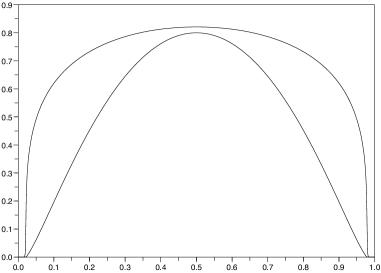
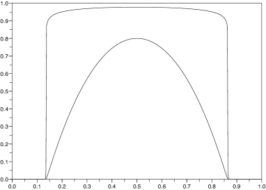
Figure 1: Effect of $m$ large. A solution to the mechanical model (1.1), (1.3) in one dimension with $\Phi(p)=5(1-p)$. Left: $m=5$. Right: $m=40$. The upper line is $\varrho$; the bottom line is $p$ (scale enlarged for visibility). Notice that the density scales are not the same in the two figures. The initial data is taken with compact support and the solution is displayed for a time large enough (see Figure 2 below for and intermediate regime).

The complementarity formula (2.7) indicates that the limit pressure at time $t$, $p_{\infty}(t)$, should solve the elliptic equation

(2.9) $$-\Delta p_{\infty}(t)=\Phi(p_{\infty}(t))\ \text{ in }\Omega(t),\qquad p_{\infty}(t)\in H^{1}_{0}\big{(}\Omega(t)\big{)},$$

a problem which is wellposed if $\Omega(t)$ is smooth enough, since $p\mapsto\Phi(p)$ is decreasing. This implies in particular that in general regularity in time for the pressure is missing, since time discontinuities may show up when two tumors meet; see Subsection A.2 in the Appendix.

Geometric motion vs. equation on the cell number density. To complete the description of the limit problem we should be able to trace $\Omega(t)$ starting from its initial position. The pressure equation (2.6) suggests that we should have

$$\partial_{t}p_{\infty}=|\nabla p_{\infty}|^{2}\quad\text{at }\partial\Omega(t),$$

which leads to a geometric motion with normal velocity $V$ at the boundary of $\Omega(t)$ given by

(2.10) $$V=|\nabla p_{\infty}|.$$

Thus we have arrived to a geometric Hele-Shaw type problem, which is the classical one when $\Phi=0$.

The above formal computation is expected to be true if we prescribe a fixed initial pressure $p_{m}(0)=p^{0}$ (which implies that the initial densities converge to the indicator function of the positivity set of $p^{0}$). When $\Phi=0$, it was proved to be true in a viscosity sense in [34]; see also [28] for an earlier result in this direction using a variational formulation of Baiocchi type.

However, if the initial densities $\varrho_{m}^{0}$ are such that $\varrho^{0}$ is below 1 in a set with positive measure, the result is no longer true. The main point is that the tumor may meet precancer zones. At a meeting point $(\overline{x},\overline{t})$, the example in Subsection A.3 in the Appendix suggests that the tumor grows faster (also for the case $\Phi=0$), with a normal velocity given by a rule of the form

(2.11) $$V=\frac{|\nabla p_{\infty}|}{1-\overline{\varrho}},$$

where $\overline{\varrho}$ is some limit of $\varrho$ as $t\to\overline{t}$ and $x\to\overline{x}$ from the outside of $\Omega(t)$. We leave open this problem, which seems to be a challenging extension of the viscosity method in [34].

Even if we consider the modified geometric motion law (2.11) instead of (2.10), the geometric formulation does not carry all the information of the limit solution. Indeed, the density in precancer zones evolves, with an exponential growth, until it reaches the level $\varrho_{\infty}=1$, a fact that is not captured neither by (2.9), nor by (2.11); see Figure 2 and the examples in the Appendix. When $\Phi=0$ we also need (2.3) to give a full description of the limit. However, in this latter case the evolution in the mushy regions is simpler, since the density does not change until it interacts with the positivity set for the pressure.

Figure 2: Cell density and pressure carry different informations. Here $m=40$ and the initial data $\varrho$ is less than $1$. The solution is displayed at four different times. It shows how the smooth part of $\varrho$ strictly less than $1$ is growing with $p=0$ (figure on the left). When $\varrho$ reaches the value $1$, the pressure becomes positive, increases and creates a moving front that delimitates the growing domain where $\varrho\approx 1$. Thin line is $\varrho$ and thick line is $p$ as functions of $x$. See also Figure 3 in the Appendix.

Let us point out that, in the case of a compactly supported initial data, precancer zones disappear in finite time.

Uniqueness. To complete the description of the asymptotic limit, we conclude with a uniqueness result, relying on a Hilbert duality method, for the free boundary problem (2.3).

Theorem 2.4

There is a unique pair $(\varrho,p)$ of functions in $L^{\infty}\big{(}(0,\infty);L^{1}(\mathbb{R}^{N})\cap L^{\infty}(\mathbb{R}^{N})\big{)}$, $\varrho\in C\big{(}[0,\infty);L^{1}(\mathbb{R}^{N})\big{)}$, $p\in P_{\infty}(\varrho)$, satisfying (2.3) and such that for all $T>0$:

• $\rho(t)$ is uniformly compactly supported for $t\in[0,T]$;

• $|\nabla p|\in L^{2}\big{(}Q_{T}\big{)}$;

• $\partial_{t}p\in M^{1}\big{(}Q_{T}\big{)}$, $\partial_{t}\varrho\in M^{1}\big{(}Q_{T}\big{)}$.

It is important to notice that if, in addition to (2.2), we assume that the initial data $\varrho^{0}_{m}$ are uniformly compactly supported, then the limit solution $(\varrho_{\infty},p_{\infty})$ to (2.3) given by Theorem 2.1 falls within the uniqueness class. As a consequence, convergence is not restricted to a subsequence.

Remark. The compact support assumption in Theorem 2.4 can be removed, to the cost of using rather technical arguments, in the style of the ones employed in the uniqueness proof for the case with nutrients, Theorem 4.2 below. We keep it for the sake of clarity.

The rest of this section is devoted to the proofs of the above mentioned results, except uniqueness, which is postponed to Section 3.

2.2 Estimates, strong limit and existence

We consider the solutions to (2.1) and proceed to obtain the estimates that allow us to pass to the limit and prove Theorem 2.1. This is a standard porous media type equation and all the manipulations below can be justified, see the monograph [42]. The main observation here is that the lower estimate on $\Delta p_{m}$ that does the job when passing to the limit in porous media equations without a source, does not work in the present case. However, a control can be obtained on the quantities $\Delta p_{m}+\Phi(p_{m})$, which will be enough for our purposes.

$L^{\infty}$ bounds for $\varrho_{m}$, $p_{m}$. Standard comparison arguments yield

$$0\leq\varrho_{m}\leq\left(\frac{m-1}{m}p_{M}\right)^{1/(m-1)}\underset{m\to\infty}{\longrightarrow}1,\qquad 0\leq p_{m}=P_{m}(\varrho_{m})\leq p_{M}.$$

This allows in particular to avoid initial layers (which are present when $\|\varrho^{0}\|_{\infty}>1$; see [29]).

$L^{1}$ bounds for $\varrho_{m}$, $p_{m}$. Let $\varrho_{m}$, $\hat{\varrho}_{m}$ be two (non-negative) solutions to (2.1), and $p_{m}=P_{m}(\varrho_{m})$, $\hat{p}_{m}=P_{m}(\hat{\varrho}_{m})$ the corresponding pressures. We have

$$\begin{array}[]{rcl}\displaystyle\frac{d}{dt}\int_{\mathbb{R}^{N}}\{\varrho_{m}(t)-\hat{\varrho}_{m}(t)\}_{+}&\leq&\displaystyle\int_{\mathbb{R}^{N}}\Phi(p_{m}(t))\{\varrho_{m}(t)-\hat{\varrho}_{m}(t)\}_{+}\\ &&+\displaystyle\int_{\mathbb{R}^{N}}\hat{\varrho}_{m}(t)(\Phi(p_{m}(t))-\Phi(\hat{p}_{m}(t)))\;\text{sign}_{+}(\varrho_{m}(t)-\hat{\varrho}_{m}(t))\\ &\leq&\displaystyle\Phi(0)\int_{\mathbb{R}^{N}}\{\varrho_{m}(t)-\hat{\varrho}_{m}(t)\}_{+},\end{array}$$

from where we get

$$\int_{\mathbb{R}^{N}}\{\varrho_{m}(t)-\hat{\varrho}_{m}(t)\}_{+}\leq\textrm{e}^{\Phi(0)t}\int_{\mathbb{R}^{N}}\{\varrho_{m}(0)-\hat{\varrho}_{m}(0)\}_{+}.$$

This “almost contraction” property yields the uniform (in $m$) bound

(2.12) $$\|\varrho_{m}(t)\|_{L^{1}(\mathbb{R}^{N})}\leq\textrm{e}^{\Phi(0)t}\|\varrho_{m}^{0}\|_{L^{1}(\mathbb{R}^{N})}\leq C\textrm{e}^{\Phi(0)t}.$$

On the other hand, $p_{m}=\frac{m}{m-1}\varrho_{m}(\frac{m-1}{m}p_{m})^{\frac{m-2}{m-1}}$. Thus, using (2.12) we conclude

$$\|p_{m}(t)\|_{L^{1}(\mathbb{R}^{N})}\leq C\textrm{e}^{\Phi(0)t}\qquad\text{for }m\geq 2.$$

A semiconvexity estimate for $p_{m}$. According to the hypotheses (1.2) on the growth function, $\displaystyle r_{\Phi}=\min_{p\in[0,p_{M}]}\left(\Phi(p)-p\Phi^{\prime}(p)\right)>0$. We will prove that

(2.13) $$\Delta p_{m}(t)+\Phi(p_{m}(t))\geq-r_{\Phi}\textrm{e}^{-(m-1)r_{\Phi}t}/(1-\textrm{e}^{-(m-1)r_{\Phi}t}).$$

As a consequence, in the limit we will have $\Delta p_{\infty}+\Phi(p_{\infty})\geq 0$.

We borrow the idea to prove inequality (2.13) from [1], where the case $\Phi=0$ was considered. We write the equation (2.6) as

(2.14) $$\partial_{t}p_{m}=(m-1)p_{m}w+|\nabla p_{m}|^{2},\quad\text{with }w=\Delta p_{m}+\Phi(p_{m}).$$

Let us denote $v=\Delta p_{m}$. Since $\Phi^{\prime}<0$, we have

$$\begin{array}[]{l}\partial_{t}v=(m-1)p_{m}\Delta w+2(m-1)\nabla p_{m}\cdot\nabla w+(m-1)vw+2\nabla p_{m}\cdot\nabla v+2\sum_{i,j}(\partial_{x_{i}x_{j}}p_{m})^{2},\\[10.0pt] \partial_{t}(\Phi(p_{m}))=\Phi^{\prime}(p_{m})\partial_{t}p_{m}=(m-1)p_{m}\Phi^{\prime}(p_{m})w+\Phi^{\prime}(p_{m})|\nabla p_{m}|^{2}\\[10.0pt] \qquad\qquad\ \,\geq(m-1)p_{m}\Phi^{\prime}(p_{m})w+2\nabla(\Phi(p_{m}))\cdot\nabla p_{m},\end{array}$$

which gives

$$\partial_{t}w\geq(m-1)p_{m}\Delta w+2m\nabla p_{m}\cdot\nabla w+(m-1)w^{2}-(m-1)\big{(}\Phi(p_{m})-p_{m}\Phi^{\prime}(p_{m})\big{)}w.$$

The function $W(t)=-r_{\Phi}\textrm{e}^{-(m-1)r_{\Phi}t}/(1-\textrm{e}^{-(m-1)r_{\Phi}t})$ is a subsolution to this equation, and (2.13) follows.

Remarks. (i) The right hand side of (2.13) behaves as $-1/(t(m-1))$ for $t\approx 0$.

(ii) For $\Phi\approx 0$ we have $r_{\Phi}\approx 0$, and we recover the well-known result for the case $\Phi=0$, namely $\Delta p_{m}(t)\geq-1/(t(m-1))$.

Bounds for $\partial_{t}p_{m}$, $\partial_{t}\varrho_{m}$. We combine (2.13) with (2.14) to obtain an estimate from below for the time derivative of the pressure,

(2.15) $$\partial_{t}p_{m}(t)\geq-(m-1)p_{m}(t)r_{\Phi}\frac{\textrm{e}^{-(m-1)r_{\Phi}t}}{1-\textrm{e}^{-(m-1)r_{\Phi}t}}\qquad\text{for }t>0.$$

This in turn gives an estimate from below for the time derivative of the density,

(2.16) $$\partial_{t}\varrho_{m}(t)\geq-\varrho_{m}(t)r_{\Phi}\frac{\textrm{e}^{-(m-1)r_{\Phi}t}}{1-\textrm{e}^{-(m-1)r_{\Phi}t}}.$$

The monotonicity inequalities (2.5) for the limit problem are then obtained just by letting $m\to\infty$ in (2.16) and (2.15).

We now use $|\partial_{t}\varrho_{m}|=\partial_{t}\varrho_{m}+2\{\partial_{t}\varrho_{m}\}_{-}$ to obtain

$$\|\partial_{t}\varrho_{m}(t)\|_{L^{1}(\mathbb{R}^{N})}=\displaystyle\frac{d}{dt}\int_{\mathbb{R}^{N}}\varrho_{m}(t)+2\int_{\mathbb{R}^{N}}\{\partial_{t}\varrho_{m}(t)\}_{-}\leq\displaystyle\left(\Phi(0)+\frac{2r_{\Phi}\textrm{e}^{-(m-1)r_{\Phi}t}}{1-\textrm{e}^{-(m-1)r_{\Phi}t}}\right)\|\varrho_{m}(t)\|_{L^{1}(\mathbb{R}^{N})}.$$

This, together with (2.12), leads to a uniform bound in space and time for time intervals of the form $t\in\left[\frac{1}{m-1},T\right]$.

An analogous computation shows that

$$\begin{array}[]{rcl}\displaystyle\int_{\frac{1}{m-1}}^{T}\int_{\mathbb{R}^{N}}|\partial_{t}p_{m}|&\leq&\displaystyle\int_{\mathbb{R}^{N}}p_{m}(T)-\int_{\mathbb{R}^{N}}p_{m}\left(\frac{1}{m-1}\right)\\[11.38109pt] &&\displaystyle+(m-1)r_{\Phi}\int_{\frac{1}{m-1}}^{T}\left(\frac{\textrm{e}^{-(m-1)r_{\Phi}t}}{1-\textrm{e}^{-(m-1)r_{\Phi}t}}\int_{\mathbb{R}^{N}}p_{m}(t)\right)\,dt\leq C(T).\end{array}$$

$L^{1}$ bounds for $\nabla\varrho_{m}$, $\nabla p_{m}$. Let $\alpha=\min_{p\in[0,p_{M}]}|\Phi^{\prime}(p)|>0$. We consider the equation for $\partial_{x_{i}}\varrho_{m}$, multiply it by $\mathop{\rm sign}(\partial_{x_{i}}\varrho_{m})=\mathop{\rm sign}(\partial_{x_{i}}p_{m})$, and use Kato’s inequality; thanks to the monotonicity of $\Phi$ we obtain

$$\begin{array}[]{rcl}\partial_{t}|\partial_{x_{i}}\varrho_{m}|-\Delta(m\varrho_{m}^{m-1}|\partial_{x_{i}}\varrho_{m}|)&\leq&\Phi(p_{m})|\partial_{x_{i}}\varrho_{m}|+\Phi^{\prime}(p_{m})\varrho_{m}|\partial_{x_{i}}p_{m}|\\[11.38109pt] &\leq&\Phi(0)|\partial_{x_{i}}\varrho_{m}|-\alpha\varrho_{m}|\partial_{x_{i}}p_{m}|.\end{array}$$

Integrating in $Q_{t}$, we get

$$\|\partial_{x_{i}}\varrho_{m}(t)\|_{L^{1}(\mathbb{R}^{N})}+\alpha\iint_{Q_{t}}\varrho_{m}|\partial_{x_{i}}p_{m}|\leq\|\partial_{x_{i}}\varrho^{0}_{m}\|_{L^{1}(\mathbb{R}^{N})}\textrm{e}^{\Phi(0)t}\leq K\textrm{e}^{\Phi(0)t},$$

which yields, on the one hand, that

$$\|\partial_{x_{i}}\varrho_{m}(t)\|_{L^{1}(\mathbb{R}^{N})}\leq K\textrm{e}^{\Phi(0)t},$$

and on the other hand that

$$\|\partial_{x_{i}}p_{m}\|_{L^{1}(Q_{T})}\leq\iint_{Q_{T}\cap\{\varrho_{m}\leq 1/2\}}m\varrho_{m}^{m-2}|\partial_{x_{i}}\varrho_{m}|+2\iint_{Q_{T}\cap\{\varrho_{m}\geq 1/2\}}\varrho_{m}|\partial_{x_{i}}p_{m}|\leq C(T).$$

Convergence and identification of the limit. Since the families $\varrho_{m}$ and $p_{m}$ are bounded in $W^{1,1}_{\rm loc}(Q)$, we have strong convergence in $L^{1}_{\rm loc}(Q)$ both for $\varrho_{m}$ and $p_{m}$.

To pass from local convergence to global convergence in $L^{1}(Q_{T})$, we need to prove that the mass in an initial strip $t\in[0,1/R]$ and in the tails $|x|>R$ are uniformly (in $m$) small if $R$ is large enough. The control on the initial strip is immediate using our uniform, in $m$ and $t$, bounds for $\|\varrho_{m}(t)\|_{L^{1}(\mathbb{R}^{N})}$ and $\|p_{m}(t)\|_{L^{1}(\mathbb{R}^{N})}$. In order to control the tails, we consider $\varphi\in C^{\infty}(\mathbb{R}^{N})$ such that $0\leq\varphi\leq 1$, $\varphi(x)=0$ for $|x|<R-1$ and $\varphi(x)=1$ for $|x|>R$, and define $\varphi_{R}(x)=\varphi(x/R)$. Then, for any $m>2$,

$$\begin{array}[]{rcl}\displaystyle\frac{d}{dt}\int_{\mathbb{R}^{N}}\varrho_{m}(t)\varphi_{R}&\leq&\displaystyle 2R^{-2}\|\varrho_{m}(t)\|^{m-1}_{L^{\infty}(\mathbb{R}^{N})}\|\varrho_{m}(t)\|_{L^{1}(\mathbb{R}^{N})}\|\Delta\varphi\|_{L^{\infty}(\mathbb{R}^{N})}+\Phi(0)\int_{\mathbb{R}^{N}}\varrho_{m}(t)\varphi_{R}\\[11.38109pt] &\leq&\displaystyle CR^{-2}+\Phi(0)\int_{\mathbb{R}^{N}}\varrho_{m}(t)\varphi_{R}.\end{array}$$

Therefore, for any $t\in[0,T]$ we have

$$\begin{array}[]{rcl}\displaystyle 0\leq\displaystyle\int_{\mathbb{R}^{N}}\varrho_{m}(t)\varphi_{R}&\leq&\displaystyle\textrm{e}^{\Phi(0)t}\left(\int_{\mathbb{R}^{N}}\varrho_{m}^{0}\varphi_{R}+CR^{-2}t\right)\\[11.38109pt] \displaystyle\hfil&\leq&\displaystyle\textrm{e}^{\Phi(0)T}\left(\|\varrho^{0}_{m}-\varrho^{0}\|_{L^{1}(\mathbb{R}^{N})}+\int_{\mathbb{R}^{N}}\varrho^{0}\varphi_{R}+CR^{-2}T\right)\leq\displaystyle\varepsilon\end{array}$$

for $R$ and $m$ are large enough. Since

$$\int_{\mathbb{R}^{N}}p_{m}(t)\varphi_{R}\leq 2\|\varrho_{m}(t)\|^{m-1}_{L^{\infty}(\mathbb{R}^{N})}\int_{\mathbb{R}^{N}}\varrho_{m}^{0}\varphi_{R}$$

for any $m\geq 2$, the tail control for the pressures follows easily.

After extraction of subsequences, we can pass to the a.e.-limit in the equation $\varrho_{m}p_{m}=p_{m}^{(1+m)/m}$ to obtain that $(1-\varrho_{\infty})p_{\infty}=0$. Passing to the limit in the estimates, we have also $0\leq\varrho_{\infty}\leq 1$, $0\leq p_{\infty}\leq p_{M}$ and $\varrho_{\infty},p_{\infty}\in BV(Q_{T})$ for all $T>0$.

All the above is enough to prove that the pair $(\varrho_{\infty},p_{\infty})$ solves the Hele-Shaw equation (2.3) but for the question of the initial data.

Time continuity and initial trace. We need delicate arguments that are fortunately in the folklore of the topic of nonlinear diffusion equations, and borrow also the conclusion from [40]. Because $\varrho_{\infty}$ is non-decreasing in time, we can write for a test function $0<\zeta(x)<1$ and $0<t_{1}<t_{2}\leq T$,

$$\begin{array}[]{rl}\displaystyle\int_{\mathbb{R}^{N}}|\varrho_{\infty}(t_{2})-\varrho_{\infty}(t_{1})|\zeta&=\displaystyle\int_{\mathbb{R}^{N}}\left[\varrho_{\infty}(t_{2})-\varrho_{\infty}(t_{1})\right]\zeta=\displaystyle\int_{t_{1}}^{t_{2}}\int_{\mathbb{R}^{N}}\left[p_{\infty}\Delta\zeta+\varrho_{\infty}\Phi(p_{\infty})\zeta\right]\\[20.0pt] &\leq C(T)(t_{2}-t_{1})\left(\|\Delta\zeta\|_{\infty}+1\right).\end{array}$$

Taking a sequence of such uniformly smooth functions that converge to $1$, we find that $\varrho_{\infty}\in C\big{(}[0,\infty);L^{1}(\mathbb{R}^{N})\big{)}$ (in fact with a locally uniform Lipschitz constant).

In order to identify the initial trace, we observe that for any test function $\zeta$ as above,

$$\int_{\mathbb{R}^{N}}\varrho_{m}(t)\zeta-\int_{\mathbb{R}^{N}}\varrho^{0}_{m}\zeta=\int_{0}^{t}\int_{\mathbb{R}^{N}}\left(p_{m}\Delta\zeta+\varrho_{m}\Phi(p_{m})\right)\zeta.$$

Letting $m\to\infty$, we have

$$\int_{\mathbb{R}^{N}}\varrho_{\infty}(t)\zeta-\int_{\mathbb{R}^{N}}\varrho^{0}_{\infty}\zeta=\int_{0}^{t}\int_{\mathbb{R}^{N}}\left(p_{\infty}\Delta\zeta+\varrho_{\infty}\Phi(p_{\infty})\right)\zeta.$$

Letting first $t\to 0$ and then $\zeta\to 1$, we conclude that $\varrho(0)=\varrho^{0}$ in $L^{1}(\mathbb{R}^{N})$.

2.3 $L^{2}$ estimates for $\nabla p_{m}$, transport equation and complementarity formula

We now prove Theorems 2.2 and 2.3, both of them connected with the fact that $\nabla p_{m}\in L^{2}(Q_{T})$ for all $T>0$.

Since we have already proved that both $\varrho_{m}$ and $p_{m}$ converge strongly in $L^{1}(Q_{T})$ for all $T>0$, the first of these theorems just depends on obtaining a uniform bound in $L^{2}(Q_{T})$ for $\nabla p_{m}$.

Proof of Theorem 2.2. We rewrite the pressure equation (2.6) as

(2.17) $$\partial_{t}p_{m}=\frac{m-1}{2}\Delta p_{m}^{2}-(m-2)|\nabla p_{m}|^{2}+(m-1)p_{m}\Phi(p_{m}).$$

Integrating in $Q_{T}$ we obtain the required estimate,

$$\|\nabla p_{m}\|_{L^{2}(Q_{T})}^{2}\leq\frac{m-1}{m-2}\Phi(0)\|p_{m}\|_{L^{1}(Q_{T})}+\frac{1}{m-2}\|p^{0}_{m}\|_{L^{1}(\mathbb{R}^{N})}.$$

$\square$

Remark. Combining (2.17) with (2.15), we obtain

$$\|\nabla p_{m}(t)\|_{L^{2}(\mathbb{R}^{N})}^{2}\leq\int_{\mathbb{R}^{N}}p_{m}(t)\left(\frac{m-1}{m-2}\Phi(0)+(m-1)r_{\Phi}\frac{\textrm{e}^{-(m-1)r_{\Phi}t}}{1-\textrm{e}^{-(m-1)r_{\Phi}t}}\right)$$

for all $m>2$. This gives a uniform estimate for $\|\nabla p_{m}(t)\|_{L^{2}(\mathbb{R}^{N})}$, $t\in\left[\tau,T\right]$, for any fixed values $0<\tau<T$. However, it does not allow to go down to $t=0$.

From the equation in (2.1) and the $L^{1}$ bound on $\partial_{t}\varrho_{m}$ we conclude that

$$\left\|\Delta\varrho_{m}^{m}(t)\right\|_{L^{1}(\mathbb{R}^{N})}\leq C\textrm{e}^{\Phi(0)t}.$$

This is an optimal bound since $p_{\infty}$ has ‘corners’ on $\partial\Omega(t)$. Because this only gives space compactness, it is not enough to establish the complementarity formula (2.7) on the pressure when passing to the limit in (2.6). We will need to perform a time regularization argument à la Steklov.

Proof of Theorem 2.3. Let $\omega_{\varepsilon}(t)\geq 0$ be a regularizing kernel in time with support $(-\varepsilon,0)$. We use the notation $\varrho_{m,\varepsilon}(t)=\omega_{\varepsilon}\star\varrho_{m}(t)=\int_{\mathbb{R}}\omega_{\varepsilon}(t-s)\varrho_{m}(s)\,ds$. The equation (2.1) gives

(2.18) $$\Delta(\varrho_{m}^{m}\star\omega_{\varepsilon})=\partial_{t}\varrho_{m,\varepsilon}-(\varrho_{m}\Phi(p_{m}))\star\omega_{\varepsilon}.$$

From here it follows that $U_{m}=\Delta(\varrho_{m}^{m}\star\omega_{\varepsilon})$ is uniformly (in $m$) smooth in time and $H^{1}$ in space for $\varepsilon$ fixed. Therefore $U_{m}$ converges strongly in $L^{1}_{\rm loc}(Q)$. Hence, after multiplying (2.18) by $p_{m}$, we may pass to the limit to obtain

$$p_{\infty}\big{(}\Delta(p_{\infty}\star\omega_{\varepsilon})+(\varrho_{\infty}\Phi(p_{\infty}))\star\omega_{\varepsilon}\big{)}=\lim_{m\to\infty}p_{m}\partial_{t}\varrho_{m,\varepsilon}.$$

In order to estimate the right hand side we make the following decomposition,

$$\begin{array}[]{l}(p_{m}\partial_{t}\varrho_{m,\varepsilon})(t)=\underbrace{\frac{m}{m-1}\int_{\mathbb{R}}\varrho_{m}^{m-1}(s)\partial_{t}\varrho_{m}(s)\omega_{\varepsilon}(t-s)ds}_{{\text{I}}_{m}(t)}\\[14.22636pt] \qquad\qquad\qquad+\underbrace{\frac{m}{m-1}\int_{\mathbb{R}}\left(\varrho_{m}^{m-1}(t)-\varrho_{m}^{m-1}(s)\right)\left(\partial_{t}\varrho_{m}(s)+\frac{C}{s}\right)\omega_{\varepsilon}(t-s)ds}_{{\text{II}}_{m}(t)}\\[14.22636pt] \qquad\qquad\qquad\underbrace{-\frac{Cm}{m-1}\int_{\mathbb{R}}\left(\varrho_{m}^{m-1}(t)-\varrho_{m}^{m-1}(s)\right)\frac{\omega_{\varepsilon}(t-s)}{s}\,ds}_{{\text{III}}_{m}(t)},\end{array}$$

where $C$ is a constant such that $\partial_{t}\varrho_{m}+\frac{C}{t}\geq 0$; see estimate (2.16).

For the first term we have

$$\int_{\mathbb{R}^{N}}|{\text{I}}_{m}(t)|\leq\frac{1}{m-1}\int_{t}^{t+\varepsilon}\omega_{\varepsilon}(t-s)\left(\int_{\mathbb{R}^{N}}|\partial_{t}\varrho_{m}^{m}(s)|\right)\,ds\leq\frac{C_{\varepsilon}}{m-1}.$$

Regarding the second term, the estimate (2.15) implies that $\partial_{t}p_{m}\geq-C$. Therefore, $\varrho_{m}^{m-1}(t)-\varrho_{m}^{m-1}(s)\leq C\varepsilon$. Let $\zeta\in\mathcal{D}^{\prime}(Q)$, and $\tau$ the smallest time in its support. Then,

$$\iint_{Q}\zeta\;{\text{II}}_{m}\leq C\varepsilon\iint_{Q}\int_{\mathbb{R}}\zeta\;\left(\partial_{t}\varrho_{m}(s)+\frac{C}{\tau}\right)\omega_{\varepsilon}(t-s)\,dsdxdt\leq C\varepsilon.$$

The third term is easy to treat. Since $s\geq t>0$, for any test function $\zeta$ as above,

$$\iint_{Q}\zeta\;{\text{III}}_{m}\underset{m\to\infty}{\longrightarrow}-C\iint_{Q}\zeta\int_{\mathbb{R}}\left(p_{\infty}(t)-p_{\infty}(s)\right)\frac{\omega_{\varepsilon}(t-s)}{s}\,dsdxdt=o(1)$$

as $\varepsilon\to 0$.

These three calculations give, in the limit $m\to\infty$,

$$p_{\infty}\big{(}\Delta(p_{\infty}\star\omega_{\varepsilon})+(\varrho_{\infty}\Phi(p_{\infty}))\star\omega_{\varepsilon}\big{)}\leq o(1)\quad\text{as }\;\varepsilon\to 0\quad\text{ in }\;\mathcal{D}^{\prime}(Q).$$

To recover the desired information,

$$p_{\infty}\big{(}\Delta p_{\infty}+\Phi(p_{\infty})\big{)}\leq 0,$$

it remains to pass to the limit as $\varepsilon\to 0$ after noticing that $p_{\infty}\varrho_{\infty}=p_{\infty}$ and that the differential term can be treated through its weak formulation; indeed, after testing it against a test function as before, it is written as

$$-\iint_{Q}\big{[}\zeta\nabla p_{\infty}\cdot\nabla(p_{\infty}\star\omega_{\varepsilon})+p_{\infty}\nabla\zeta\cdot\nabla(p_{\infty}\star\omega_{\varepsilon})\big{]}$$

which passes to the limit $\varepsilon\to 0$ because we already know that $\nabla p_{\infty}\in L^{2}(Q_{T})$. Therefore,

$$-\iint_{Q}\big{[}\zeta|\nabla p_{\infty}|^{2}+p_{\infty}\nabla\zeta\cdot\nabla p_{\infty}+\zeta p_{\infty}\Phi(p_{\infty})\big{]}=0.$$

$\square$

As we have already mentioned, the complementarity formula is equivalent to the strong convergence of the gradients.

Lemma 2.5

The complementarity formula (2.8) holds if and only if $\nabla p_{m}\underset{m\to\infty}{\longrightarrow}\nabla p_{\infty}$ strongly in $L^{2}(Q_{T})$ for all $T>0$,

Proof. We consider a test function $\zeta\in\mathcal{D}^{\prime}(Q)$ and use (2.14) and (2.3) to obtain

$$\iint_{Q}\zeta p_{m}(\Delta p_{m}+\Phi(p_{m}))=\frac{1}{m-1}\iint_{Q}\zeta\left(\partial_{t}p_{m}-|\nabla p_{m}|^{2}\right)\underset{m\to\infty}{\longrightarrow}0.$$

This implies, after an integration by parts, that

$$\iint_{Q}\left[-\zeta|\nabla p_{m}|^{2}-p_{m}\nabla\zeta\cdot\nabla p_{m}+p_{m}\zeta\Phi(p_{m})\right]\underset{m\to\infty}{\longrightarrow}0.$$

Let $r=\liminf_{m\to\infty}\iint_{Q}\zeta|\nabla p_{m}|^{2}-\iint_{Q}\zeta|\nabla p_{\infty}|^{2}$. Thanks to Fatou’s Lemma, $r\geq 0$. On the other hand, since $p_{m}$ converges strongly, after extraction of subsequences we have

$$\iint_{Q}\left[-\zeta|\nabla p_{\infty}|^{2}-p_{\infty}\nabla\zeta\cdot\nabla p_{\infty}+\zeta p_{\infty}\Phi(p_{\infty})\right]=r,$$

and $r=0$ is equivalent to the strong convergence. $\square$

2.4 Finite speed of propagation

If the initial data are compactly supported uniformly in $m$, we can control the supports of $p_{m}(t)$ and $\varrho_{m}(t)$ uniformly in $m$ and $t\in[0,T]$ for all $T>0$. This implies that the speed of propagation is finite for the limit problem.

The control is performed comparing the pressures with functions of the form

(2.19) $$P(x,t)=\left(C-\frac{|x|^{2}}{4(\tau+t)}\right)_{+}.$$

The key point is that these functions, which are viscosity solutions of the Hamilton-Jacobi equation $P_{t}=|\nabla P|^{2}$, are supersolutions to the equation

(2.20) $$\partial_{t}p=(m-1)p\Delta p+|\nabla p|^{2}+(m-1)p\Phi(0)$$

for some time interval which does not depend on $m$. This idea was already used for the case $\Phi=0$ in [28, 29]. However, in the absence of reaction, $P$ is a supersolution for all times, and the proof is a bit easier.

Lemma 2.6

Let $\{\varrho_{m}^{0}\}$ satisfying (2.2) and such that all their supports are contained in a common ball $B_{R}$. Then, for every $T>0$, there is a radius $\mathcal{R}_{T}$ depending only on $\sup_{m}\|\varrho_{m}^{0}\|_{L^{\infty}(\mathbb{R}^{N})}$, $R$ and $T$, such that the supports of $\{\varrho_{m}(t)\}$ are contained in the ball $B_{\mathcal{R}_{T}}$ for all $m>1$ and $t\in[0,T]$.

Proof. We consider $P$ as in (2.19) with $\tau=N/(4\Phi(0))$ and $C$ large enough so that $P(x,0)\geq\varrho_{m}^{0}(x)$ for all $x\in\mathbb{R}^{N}$ and $m>1$. An easy computation shows that

$$\partial_{t}P-(m-1)P\Delta P-|\nabla P|^{2}-(m-1)P\Phi(0)=(m-1)P(x,t)\left(\frac{N}{2(\tau+t)}-\Phi(0)\right)\geq 0$$

for all $t\in[0,\frac{N}{4\Phi(0)}]$. Since the functions $p_{m}$ are subsolutions to (2.20), we conclude that the supports of the functions $\varrho_{m}$ are contained in the ball of radius $\sqrt{\frac{2CN}{\Phi(0)}}$ for all $t\in[0,\frac{N}{4\Phi(0)}]$. Moreover, $\|p_{m}(\frac{N}{4\Phi(0)})\|_{L^{\infty}(\mathbb{R}^{N})}\leq C$, and the argument can be iterated to reach the time $T$ in a finite number of steps. $\square$

3 Uniqueness for the purely mechanical limit problem

In this section we prove, under suitable assumptions, that the limit problem (2.3) has a unique solution, Theorem 2.4. The main difficulty comes from the fact that $p$ is not a Lipschitz, single-valued function of $\varrho$. Hence, we cannot apply directly the ideas developed in [7] to adapt Hilbert’s duality method to the porous medium equation. The technique has to be modified, in the spirit of [17].

Dual problem. Consider two solutions, $(\varrho_{1},p_{1})$, $(\varrho_{2},p_{2})$. Let $\Omega$ be a bounded domain containing the supports of both solutions for all $t\in[0,T]$, and $\Omega_{T}=\Omega\times(0,T)$. Then we have

(3.1) $$\iint_{\Omega_{T}}\big{[}(\varrho_{1}-\varrho_{2})\partial_{t}\psi+(p_{1}-p_{2})\Delta\psi+(\varrho_{1}\Phi(p_{1})-\varrho_{2}\Phi(p_{2}))\psi\big{]}=0$$

for all suitable test functions $\psi$. This can be rewritten as

(3.2) $$\iint_{\Omega_{T}}(\varrho_{1}-\varrho_{2}+p_{1}-p_{2})\left[A\partial_{t}\psi+{B}\Delta\psi+A\Phi(p_{1})\psi-C{B}\psi\right]=0,$$

where, for some fixed $\nu>0$,

$$\begin{array}[]{l}0\leq\displaystyle A=\frac{\varrho_{1}-\varrho_{2}}{(\varrho_{1}-\varrho_{2})+(p_{1}-p_{2})}\leq 1,\\[10.0pt] 0\leq\displaystyle B=\frac{p_{1}-p_{2}}{(\varrho_{1}-\varrho_{2})+(p_{1}-p_{2})}\leq 1,\\[10.0pt] 0\leq\displaystyle C=\;-\varrho_{2}\,\frac{\Phi(p_{1})-\Phi(p_{2})}{p_{1}-p_{2}}\;\leq\nu.\end{array}$$

To arrive to these bounds on $A$ and $B$, we define $A=0$ when $\varrho_{1}=\varrho_{2}$, even when $p_{1}=p_{2}$, and $B=0$ when $p_{1}=p_{2}$, even when $\varrho_{1}=\varrho_{2}$.

The idea of Hilbert’s duality method is to solve the dual problem

$$\left\{\begin{array}[]{l}A\partial_{t}\psi+{B}\Delta\psi+A\Phi(p_{1})\psi-C{B}\psi=AG\quad\text{in }\Omega_{T},\\[10.0pt] \psi=0\quad\text{in }\partial\Omega\times(0,T),\quad\psi(\cdot,T)=0\quad\text{in }\Omega,\end{array}\right.$$

for any smooth function $G$, and use $\psi$ as test function. This would yield

$$\iint_{\Omega_{T}}(\varrho_{1}-\varrho_{2})G=0,$$

from where uniqueness for the density is immediate. Uniqueness for the pressure would then follow from (3.1).

However, on the one hand the coefficients of the dual problem are not smooth, and, on the other, since $A$ and $B$ are not strictly positive, the dual equation is not uniformly parabolic. A smoothing argument is required.

Regularized dual problem. Let $\{A_{n}\}$, $\{B_{n}\}$, $\{C_{n}\}$, $\{\Phi_{1,n}\}$ be sequences of smooth bounded functions such that

$$\left\{\begin{array}[]{lll}\|A-A_{n}\|_{L^{2}(\Omega_{T})}<\alpha/n,&1/n<A_{n}\leq 1,\\[8.53581pt] \|B-B_{n}\|_{L^{2}(\Omega_{T})}<\beta/n,&1/n<B_{n}\leq 1,\\[8.53581pt] \|C-C_{n}\|_{L^{2}(\Omega_{T})}<\delta_{1}/n,&0\leq C_{n}<M_{1},&\|\partial_{t}C_{n}\|_{L^{1}(\Omega_{T})}\leq K_{1}\\[8.53581pt] \|\Phi(p_{1})-\Phi_{1,n}\|_{L^{2}(\Omega_{T})}<\delta_{2}/n,&|\Phi_{1,n}|<M_{2},&\|\nabla\Phi_{1,n}\|_{L^{2}(\Omega_{T})}\leq K_{2},\end{array}\right.$$

for some constants $\alpha,\beta,\delta_{1},\delta_{2},M_{1},M_{2},K_{1},K_{2}$.

For any smooth function $G$, we consider the solution $\psi_{n}$ of the backward heat equation

(3.3) $$\left\{\begin{array}[]{l}\displaystyle\partial_{t}\psi_{n}+\frac{B_{n}}{A_{n}}\Delta\psi_{n}+\Phi_{1,n}\psi_{n}-C_{n}\frac{B_{n}}{A_{n}}\psi_{n}=G\quad\text{in }\Omega_{T},\\[10.0pt] \psi_{n}=0\quad\text{in }\partial\Omega\times(0,T),\quad\psi_{n}(\cdot,T)=0\quad\text{in }\Omega.\end{array}\right.$$

The coefficient $B_{n}/A_{n}$ is continuous, positive and bounded below away from zero. Thus, the equation satisfied by $\psi_{n}$ is uniformly parabolic in $\Omega_{T}$. Hence $\psi_{n}$ is smooth and can be used as a test function in (3.2).

Combining (3.2) and (3.3), we have

$$\iint_{\Omega_{T}}(\varrho_{1}-\varrho_{2})G=I^{1}_{n}-I^{2}_{n}-I^{3}_{n}+I^{4}_{n},$$

where

$$\begin{array}[]{l}I^{1}_{n}=\displaystyle\iint_{\Omega_{T}}\big{(}(\varrho_{1}-\varrho_{2})+(p_{1}-p_{2})\big{)}\frac{B_{n}}{A_{n}}(A-A_{n})\left(\Delta\psi_{n}-C_{n}\psi_{n}\right),\\[10.0pt] I^{2}_{n}=\displaystyle\iint_{\Omega_{T}}\big{(}(\varrho_{1}-\varrho_{2})+(p_{1}-p_{2})\big{)}(B-B_{n})\left(\Delta\psi_{n}-C_{n}\psi_{n}\right),\\[10.0pt] I^{3}_{n}=\displaystyle\iint_{\Omega_{T}}(\varrho_{1}-\varrho_{2})(\Phi(p_{1})-\Phi_{1,n})\psi_{n},\\[10.0pt] I^{4}_{n}=\displaystyle\iint_{\Omega_{T}}\big{(}(\varrho_{1}-\varrho_{2})+(p_{1}-p_{2})\big{)}B(C-C_{n})\psi_{n}.\end{array}$$

Limit $n\to\infty$. Uniform bounds and conclusion. Our aim is to prove that $\lim_{n\to\infty}I^{i}_{n}=0$, $i=1,\dots,4$, which implies that $\varrho_{1}=\varrho_{2}$. For this task we will use some bounds that we gather in the following lemma.

Lemma 3.1

There are constants $\kappa_{i}$, $i=1,2,3$, depending on $T$ and $G$, but not on $n$, such that

$$\|\psi_{n}\|_{L^{\infty}(\Omega_{T})}\leq\kappa_{1},\quad\sup_{0\leq t\leq T}\|\nabla\psi_{n}(t)\|_{L^{2}(\Omega)}\leq\kappa_{2},\quad\|(B_{n}/A_{n})^{1/2}\left(\Delta\psi_{n}-C_{n}\psi_{n}\right)\|_{L^{2}(\Omega_{T})}\leq\kappa_{3}.$$

Proof. The first bound is just the maximum principle because $C_{n}$ is non-negative and $\Phi_{1,n}$ uniformly bounded.

The second bound is obtained multiplying the equation in (3.3) by $\Delta\psi_{n}-C_{n}\psi_{n}$. After integration in $\Omega\times(t,T)$, we get

(3.4) $$\begin{array}[]{l}\displaystyle\frac{1}{2}\|\nabla\psi_{n}(t)\|_{L^{2}(\Omega)}^{2}+\int_{t}^{T}\int_{\Omega}\frac{B_{n}}{A_{n}}|\Delta\psi_{n}-C_{n}\psi_{n}|^{2}=-\int_{\Omega}\left(\frac{C_{n}\psi_{n}^{2}}{2}\right)(t)\\[11.38109pt] \displaystyle\quad+\int_{t}^{T}\int_{\Omega}\left[-\partial_{t}C_{n}\frac{\psi_{n}^{2}}{2}-\Phi_{1,n}|\nabla\psi_{n}|^{2}-\psi_{n}\nabla\Phi_{1,n}\cdot\nabla\psi_{n}+C_{n}\Phi_{1,n}\psi_{n}^{2}+\psi_{n}\Delta G-GC_{n}\psi_{n}\right]\\[11.38109pt] \displaystyle\ \leq K\left(1-t+\int_{t}^{T}\|\nabla\psi_{n}(s)\|_{L^{2}(\Omega)}^{2}\,ds\right),\end{array}$$

where we denote by $K$ various constants independent of $n$. We now use the Grönwall lemma to conclude our second uniform bound. Then we can use again the inequality (3.4) to conclude the third one.   $\square$

We now get

$$\begin{array}[]{rcl}\displaystyle|I^{1}_{n}|&\leq&\displaystyle K\iint_{\Omega_{T}}\frac{B_{n}}{A_{n}}|A-A_{n}|\,|\Delta\psi_{n}-C_{n}\psi_{n}|\leq K\|(B_{n}/A_{n})^{1/2}(A-A_{n})\|_{L^{2}(\Omega_{T})}\\[10.0pt] &\leq&\displaystyle Kn^{1/2}\|A-A_{n}\|_{L^{2}(\Omega_{T})}\leq K\alpha/n^{1/2};\\[10.0pt] \displaystyle|I^{2}_{n}|&\leq&\displaystyle K\iint_{\Omega_{T}}|B-B_{n}|\,|\Delta\psi_{n}-C_{n}\psi_{n}|\leq K\|(A_{n}n^{1/2}/B_{n})^{1/2}(B-B_{n})\|_{L^{2}(\Omega_{T})}\\[10.0pt] &\leq&\displaystyle Kn^{1/2}\|B-B_{n}\|_{2}\leq K\beta/n^{1/2};\\[10.0pt] \displaystyle|I^{3}_{n}|&\leq&\displaystyle\iint_{\Omega_{T}}|\varrho_{1}-\varrho_{2}|\,|\Phi(p_{1})-\Phi_{1,n}|\,|\psi_{n}|\leq K\|\Phi(p_{1})-\Phi_{1,n}\|_{L^{2}(\Omega_{T})}\leq K\delta_{2}/n;\\[10.0pt] \displaystyle|I^{4}_{n}|&\leq&\displaystyle K\iint_{\Omega_{T}}B|C-C_{n}|\,|\psi_{n}|\leq\displaystyle K\|C-C_{n}\|_{L^{2}(\Omega_{T})}\leq K/n.\end{array}$$

Once we have proved that $\varrho_{1}=\varrho_{2}$, equation (3.1) says that

$$\iint_{\Omega_{T}}\ \big{[}(p_{1}-p_{2})\Delta\psi+\varrho_{1}(\Phi(p_{1})-\Phi(p_{2}))\psi\big{]}=0,$$

from where the result will follow by taking as test function $\psi=p_{1}-p_{2}$, using the monotonicity of $\Phi$.

4 Model with nutrients

When nutrients are taken into account, we are led to problem (1.4). We again assume that the pressure field is given by (1.3), with $\varrho_{c}$ set equal to 1.

Our assumptions on the initial data are stronger than for the purely mechanical problem. Namely, in addition to (2.2), we assume that for some $c^{0}$ such that $c_{B}-c^{0}\in L^{1}_{+}(\mathbb{R}^{N})$,

(4.1) $$\left\{\begin{array}[]{l}0\leq c_{m}^{0}<c_{B},\quad\|c_{m}^{0}-c^{0}\|_{L^{1}(\mathbb{R}^{N})}\underset{m\to\infty}{\longrightarrow}0,\quad\|(c_{m}^{0})_{x_{i}}\|_{L^{1}(\mathbb{R}^{N})}\leq C,\quad i=1,\dots,N,\\[8.0pt] \|{\rm div}(\varrho_{m}^{0}\nabla p_{m}^{0})+\varrho_{m}^{0}\;\Phi(p_{m}^{0},c_{m}^{0})\|_{L^{1}(\mathbb{R}^{N})}\leq C,\quad\|\Delta c_{m}^{0}-\varrho_{m}^{0}\;\Psi(p_{m}^{0},c_{m}^{0})\|_{L^{1}(\mathbb{R}^{N})}\leq C.\end{array}\right.$$

An interesting difference with the purely mechanical model is that when nutrients are not enough the cells might die (or become quiescent), which is represented by $\Phi(p,c)<0$ for $c$ small enough with $p$ given. These cells, which are in principle in the center of the tumor, are replaced by cells from the boundary moving inwards by pressure forces. In particular the growth inequalities (2.5) cannot hold true here.

A typical choice is $\Psi(c,p)=c$, $\Phi(c,p)=\widetilde{\Phi}(p)(c+\widetilde{c}_{1})-\widetilde{c}_{2}$ with $\widetilde{c}_{i}>0$ two constants and $\widetilde{\Phi}(p)$ a function having the same properties as in the purely fluid mechanical model.

4.1 Main results

As in the case without nutrients, in the limit we obtain a free boundary problem of Hele-Shaw type.

Theorem 4.1

Let $\Phi$, $\Psi$ satisfy (1.5), and $\{(\varrho_{m}^{0},c^{0}_{m})\}$ satisfy the hypotheses (2.2) and (4.1). Then, after extraction of subsequences, the density $\varrho_{m}$, the nutrient $c_{m}$ and the pressure $p_{m}$ converge for all $T>0$ strongly in $L^{1}(Q_{T})$ as $m\to\infty$ to limits $\varrho_{\infty},c_{\infty},p_{\infty}\in BV(Q_{T})$ that satisfy $0\leq\varrho_{\infty}\leq 1$, $0\leq c_{\infty}\leq c_{B}$ and $0\leq p_{\infty}\leq p_{M}$, and

(4.2) $$\left\{\begin{array}[]{ll}\displaystyle\partial_{t}\varrho_{\infty}=\Delta p_{\infty}+\varrho_{\infty}\Phi(p_{\infty},c_{\infty}),&\displaystyle\varrho_{\infty}(0)=\varrho^{0},\\[11.38109pt] \displaystyle\partial_{t}c_{\infty}=\Delta c_{\infty}-\varrho_{\infty}\Psi(p_{\infty},c_{\infty})&c_{\infty}(0)=c^{0},\end{array}\right.$$

in a distributional sense, plus the relation $p_{\infty}\in P_{\infty}(\varrho_{\infty})$, where $P_{\infty}$ is the Hele-Shaw graph (2.4).

When we say that $(\varrho_{\infty},p_{\infty},c_{\infty})$ is a solution to (4.2) in a distributional sense, we mean that

$$\begin{array}[]{ll}\displaystyle\iint_{Q}\big{\{}\varrho_{\infty}\psi_{t}+p_{\infty}\Delta\psi+\varrho_{\infty}\Phi(p_{\infty},c_{\infty})\psi\big{\}}=-\int_{\mathbb{R}^{N}}\varrho^{0}\psi(\cdot,0),\\[11.38109pt] \displaystyle\iint_{Q}\big{\{}c_{\infty}\zeta_{t}+c_{\infty}\Delta\zeta-\varrho_{\infty}\Psi(p_{\infty},c_{\infty})\zeta\big{\}}=-\int_{\mathbb{R}^{N}}c^{0}\zeta(\cdot,0),\end{array}$$

for all test functions $\psi,\zeta\in C^{\infty}_{0}(\overline{Q})$.

As mentioned above, for the system we lose the monotonicity properties (2.5), and we are not able to prove the expected continuity of $\varrho_{\infty}$ and $c_{B}-c_{\infty}$ in $L^{1}(\mathbb{R}^{N})$. However, we are still able to prove that $\nabla p_{\infty}$ in $L^{2}(Q_{T})$. Therefore, the equation on the cell density can also be written as a transport equation,

(4.3) $$\partial_{t}\varrho_{\infty}-{\rm div}\left(\varrho_{\infty}\nabla p_{\infty}\right)=\varrho_{\infty}\Phi(p_{\infty},c_{\infty}).$$

If the initial data $\varrho_{m}^{0}$ are compactly supported uniformly in $m$, we can control the supports of $\varrho_{m}(t)$ uniformly in $m$ for each $t>0$. Hence, in the limit problem tumors propagate with a finite speed (this is not true for the nutrients), and a free boundary shows up. This can be proved through a comparison argument with the same barrier functions as in the scalar case. Moreover, the constructed solution will fall within a class for which we prove uniqueness.

Theorem 4.2

There is a unique triple $(\varrho,p,c)$, $\varrho,p,c_{B}-c\in L^{\infty}((0,\infty);L^{1}(\mathbb{R}^{N})\cap L^{\infty}(\mathbb{R}^{N}))$, $p\in P_{\infty}(\varrho)$, satisfying (4.2) in the distributional sense and such that for all $T>0$:

• $\rho(t)$ is uniformly compactly supported for $t\in[0,T]$;

• $|\nabla c|,|\nabla p|\in L^{2}(Q_{T})$;

• $\partial_{t}p\in M^{1}(Q_{T})$, $\partial_{t}\varrho\in M^{1}(Q_{T})$.

As in the purely mechanical model, we can write an equation for the pressure $p_{m}$,

(4.4) $$\partial_{t}p_{m}=(m-1)p_{m}\Delta p_{m}+|\nabla p_{m}|^{2}+(m-1)p_{m}\Phi(p_{m},c_{m}).$$

This suggests that the complementarity formula

(4.5) $$p_{\infty}\left(\Delta p_{\infty}+\Phi(p_{\infty},c_{\infty})\right)=0$$

holds. However, we have not been able to establish it rigorously. The reason is that, in contrast with the case without nutrients, we have failed to control $\Delta p_{m}+\Phi(p_{m},c_{m})$ from below by means of a comparison argument, or to prove the strong convergence of $\nabla p_{m}$ in $L^{2}(Q_{T})$ for all $T>0$. We leave open the question to give conditions on $\Phi(p,c)$ allowing to prove formula (4.5).

The rest of this section is devoted to prove the first of these theorems. The uniqueness result is postponed to a later section.

4.2 Estimates

$L^{\infty}$ bounds for $\varrho_{m}$, $p_{m}$, $c_{m}$. The assumptions on the growth functions (1.5) imply, using standard comparison arguments,

$$0\leq\varrho_{m}\leq\left(\frac{m-1}{m}p_{M}\right)^{1/(m-1)},\qquad 0\leq p_{m}(x,t)\leq p_{M},\qquad 0<c_{m}<c_{B}.$$

$L^{1}$ bounds for $\varrho_{m}$, $p_{m}$, $c_{m}$. Let $(\varrho,c)$ and $(\hat{\varrho},\hat{c})$ be two solutions of the system for a fixed $m$, with corresponding pressures $p$ and $\hat{p}$. We subtract the equation for $\hat{\varrho}$ from the equation for $\varrho$, and multiply the resulting equation by $\mathop{\rm sign}(\varrho-\hat{\varrho})$, and do an analogous manipulation for the $c$ variable. We integrate by parts, and obtain

$$\left\{\begin{array}[]{l}\displaystyle\frac{d}{dt}\|(\varrho-\hat{\varrho})(t)\|_{L^{1}(\mathbb{R}^{N})}\leq\int_{\mathbb{R}^{N}}\Big{[}\big{(}\varrho\Phi(p,c)-\hat{\varrho}\Phi(\hat{p},\hat{c})\big{)}\mathop{\rm sign}(p-\hat{p})\Big{]}(t),\\[10.0pt] \displaystyle\frac{d}{dt}\|(c-\hat{c})(t)\|_{L^{1}(\mathbb{R}^{N})}\leq-\int_{\mathbb{R}^{N}}\Big{[}\big{(}\varrho\Psi(p,c)-\hat{\varrho}\Psi(\hat{p},\hat{c})\big{)}\mathop{\rm sign}(c-\hat{c})\Big{]}(t).\end{array}\right.$$

Let $\mu$ be a positive constant to be chosen later. We have

$$\begin{array}[]{l}\displaystyle\frac{d}{dt}\Big{(}\|(\varrho-\hat{\varrho})(t)\|_{L^{1}(\mathbb{R}^{N})}+\mu\|(c-\hat{c})(t)\|_{L^{1}(\mathbb{R}^{N})}\Big{)}\leq\\[11.38109pt] \quad\displaystyle\underbrace{\int_{\mathbb{R}^{N}}\Big{[}\big{(}\varrho-\hat{\varrho}\big{)}\big{(}\Phi(p,c)\mathop{\rm sign}(\varrho-\hat{\varrho})-\mu\Psi(p,c)\mathop{\rm sign}(c-\hat{c})\big{)}\Big{]}(t)}_{\mathcal{I}}\\[11.38109pt] \quad+\underbrace{\int_{\mathbb{R}^{N}}\Big{[}\hat{\varrho}\big{(}(\Phi(p,c)-\Phi(p,\hat{c}))\mathop{\rm sign}(\varrho-\hat{\varrho})-\mu(\Psi(p,c)-\Psi(p,\hat{c}))\mathop{\rm sign}(c-\hat{c})\big{)}\Big{]}(t)}_{\mathcal{J}}\\[11.38109pt] \quad+\underbrace{\int_{\mathbb{R}^{N}}\Big{[}\hat{\varrho}\big{(}(\Phi(p,\hat{c})-\Phi(\hat{p},\hat{c}))\mathop{\rm sign}(\varrho-\hat{\varrho})-\mu(\Psi(p,\hat{c})-\Psi(\hat{p},\hat{c}))\mathop{\rm sign}(c-\hat{c})\big{)}\Big{]}(t)}_{\mathcal{K}}.\end{array}$$

Let $A=\{0\leq p\leq p_{M},\,0\leq c\leq c_{B}\}$, $\alpha=\min_{A}|\partial_{p}\Phi|>0$, $\beta=\max_{A}|\partial_{p}\Psi|$. Since $\partial_{p}\Phi<0$, if $\displaystyle 0<\mu\leq\alpha/\beta$, there are constants $C$ independent of $m$ such that

$$\begin{array}[]{l}\mathcal{I}\leq\displaystyle\int_{\mathbb{R}^{N}}\Big{[}|\varrho-\hat{\varrho}|\left(\Phi(p,c)+\mu\Psi(p,c)\right)\Big{]}(t)\leq C\|(\varrho-\hat{\varrho})(t)\|_{L^{1}(\mathbb{R}^{N})},\\[11.38109pt] \displaystyle\mathcal{J}\leq\|\hat{\rho}\|_{L^{\infty}(Q)}\left(\|\partial_{c}\Phi\|_{L^{\infty}(A)}+\mu\|\partial_{c}\Psi\|_{L^{\infty}(A)}\right)\|(c-\hat{c})(t)\|_{L^{1}(\mathbb{R}^{N})}\leq C\|(c-\hat{c})(t)\|_{L^{1}(\mathbb{R}^{N})},\\[11.38109pt] \displaystyle\mathcal{K}\leq\int_{\mathbb{R}^{N}}\Big{[}\hat{\varrho}\big{(}-\big{|}\Phi(p,\hat{c})-\Phi(\hat{p},\hat{c})\big{|}+\mu\big{|}\Psi(p,\hat{c})-\Psi(\hat{p},\hat{c})\big{|}\big{)}\Big{]}(t)\leq 0.\end{array}$$

We conclude that

$$\frac{d}{dt}\Big{(}\|(\varrho-\hat{\varrho})(t)\|_{L^{1}(\mathbb{R}^{N})}+\mu\|(c-\hat{c})(t)\|_{L^{1}(\mathbb{R}^{N})}\Big{)}\leq C\Big{(}\|(\varrho-\hat{\varrho})(t)\|_{L^{1}(\mathbb{R}^{N})}+\mu\|(c-\hat{c})(t)\|_{L^{1}(\mathbb{R}^{N})}\Big{)}.$$

Therefore,

$$\|(\varrho-\hat{\varrho})(t)\|_{L^{1}(\mathbb{R}^{N})}+\mu\|(c-\hat{c})(t)\|_{L^{1}(\mathbb{R}^{N})}\leq\textrm{e}^{Ct}\Big{(}\|\varrho^{0}-\hat{\varrho}^{0}\|_{L^{1}(\mathbb{R}^{N})}+\mu\|c^{0}-\hat{c}^{0}\|_{L^{1}(\mathbb{R}^{N})}\Big{)}.$$

This gives uniqueness, and choosing $(\varrho,c)=(\varrho_{m},c_{m})$, and $(\hat{\varrho},\hat{c})=(0,c_{B})$, we find the uniform estimates

(4.6) $$\|\varrho_{m}(t)\|_{L^{1}(\mathbb{R}^{N})},\quad\|c_{m}(t)-c_{B}\|_{L^{1}(\mathbb{R}^{N})}\leq K\textrm{e}^{Ct}.$$

As in the purely fluid mechanical model, from the $L^{\infty}$ bounds and (4.6), we conclude that, for $m>2$,

$$\|p_{m}(t)\|_{L^{1}(\mathbb{R}^{N})}\leq K\textrm{e}^{Ct}.$$

$L^{1}$ bounds on the derivatives of $\varrho_{m}$ and $c_{m}$. We differentiate the two equations of the system with respect to time, multiply the first one by $\text{sign}(\partial_{t}\varrho_{m})$ and the second by $\text{sign}(\partial_{t}c_{m})$ and use Kato’s inequality to obtain

(4.7) $$\left\{\begin{array}[]{l}\displaystyle\partial_{t}|\partial_{t}\varrho_{m}|-\Delta(m\varrho_{m}^{m-1}|\partial_{t}\varrho_{m}|)\leq|\partial_{t}\varrho_{m}|\Phi+\varrho_{m}\partial_{p}\Phi|\partial_{t}p_{m}|+\varrho_{m}\partial_{c}\Phi\partial_{t}c_{m}\mathop{\rm sign}(\partial_{t}\varrho_{m}),\\[10.0pt] \displaystyle\partial_{t}|\partial_{t}c_{m}|-\Delta(|\partial_{t}c_{m}|)\leq-\partial_{t}\varrho_{m}\Psi\mathop{\rm sign}(\partial_{t}c_{m})-\varrho_{m}\partial_{p}\Psi\partial_{t}p_{m}\mathop{\rm sign}(\partial_{t}c_{m})-\varrho_{m}\partial_{c}\Psi|\partial_{t}c_{m}|.\end{array}\right.$$

We integrate in space and add the two equations to obtain, using the monotonicity properties of the growth functions,

$$\begin{gathered}\frac{d}{dt}\Big{(}\|\partial_{t}\varrho_{m}(t)\|_{L^{1}(\mathbb{R}^{N})}+\mu\|\partial_{t}c_{m}(t)\|_{L^{1}(\mathbb{R}^{N})}\Big{)}\leq\\[11.38109pt] \int_{\mathbb{R}^{N}}\left(|\partial_{t}\varrho_{m}(t)|\big{(}\Phi+\mu\Psi\big{)}(0,c_{B})+\|\varrho_{m}\|_{L^{\infty}(Q)}\|\partial_{c}\Phi\|_{L^{\infty}(A)}|\partial_{t}c_{m}(t)|\right),\end{gathered}$$

and thus, thanks to assumption (4.1),

$$\|\partial_{t}\varrho_{m}(t)\|_{L^{1}(\mathbb{R}^{N})}+\|\partial_{t}c_{m}(t)\|_{L^{1}(\mathbb{R}^{N})}\leq C\textrm{e}^{Ct}\Big{(}\|(\partial_{t}\varrho)^{0}\|_{L^{1}(\mathbb{R}^{N})}+|(\partial_{t}c)^{0}\|_{L^{1}(\mathbb{R}^{N})}\Big{)}=K\textrm{e}^{Ct}.$$

We can estimate the space derivatives in the same way, and arrive to

$$\|\partial_{x_{i}}\varrho_{m}(t)\|_{L^{1}(\mathbb{R}^{N})}+\|\partial_{x_{i}}c_{m}(t)\|_{L^{1}(\mathbb{R}^{N})}\leq K\textrm{e}^{Ct},\qquad i=1,\dots,N.$$

Estimates on the derivatives of $p_{m}$. From the first equation in (4.7), using the strict monotonicity of $\Phi$ with respect to $p$ and the $BV$ estimates that we have already proved, we get

$$\int_{\mathbb{R}^{N}}|\partial_{t}\varrho_{m}(T)|+\alpha\iint_{Q_{T}}\varrho_{m}|\partial_{t}p_{m}|\leq K\textrm{e}^{CT},$$

where, as above, $\alpha=\min_{A}|\partial_{p}\Phi|>0$. Therefore,

$$\|\partial_{t}p_{m}\|_{L^{1}(Q_{T})}\leq\iint_{Q_{T}\cap\{\varrho\leq 1/2\}}m\varrho_{m}^{m-2}|\partial_{t}\varrho_{m}|+2\iint_{Q_{T}\cap\{\varrho_{m}\geq 1/2\}}\varrho_{m}|\partial_{t}p_{m}|\leq C(T).$$

The control on the space derivatives follows by a similar argument, and we obtain

$$\|\partial_{x_{i}}p_{m}\|_{L^{1}(Q_{T})}\leq C(T),\quad i=1,\dots,N.$$

Convergence and identification of the limit. The above estimates give strong convergence in $L^{1}_{\rm loc}(Q)$ for $\varrho_{m}$, $c_{B}-c_{m}$ and $p_{m}$. Our uniform control of the $L^{1}$ norms of these quantities in $m$ and $t\in[0,T]$ shows that the mass in thin initial strips is uniformly in $m$ small. Therefore, to get global convergence in $L^{1}(Q_{T})$, we just need to control the tails. Proceeding as in the case without nutrients, we get

$$\frac{d}{dt}\int_{\mathbb{R}^{N}}\varrho_{m}(t)\varphi_{R}\leq CR^{-2}+\Phi(0,c_{B})\int_{\mathbb{R}^{N}}\varrho_{m}(t)\varphi_{R},$$

from where the tail control for $\varrho_{m}$, and then for $p_{m}$, follows easily.

As for the nutrients, we have

$$\frac{d}{dt}\int_{\mathbb{R}^{N}}(c_{B}-c_{m}(t))\varphi_{R}\leq R^{-2}\|\Delta\varphi\|_{L^{\infty}(\mathbb{R}^{N})}\int_{\mathbb{R}^{N}}(c_{B}-c_{m}(t))+\Psi(0,c_{B})\int_{\mathbb{R}^{N}}\varrho_{m}(t)\varphi_{R}.$$

But we already have a tail control for $\varrho_{m}$. Hence, for all $R$ and $m$ large enough,

$$\int_{\mathbb{R}^{N}}(c_{B}-c_{m}(t))\varphi_{R}\leq\int_{\mathbb{R}^{N}}(c_{B}-c^{0}(t))\varphi_{R}+\int_{\mathbb{R}^{N}}|c^{0}(t)-c^{0}_{m}(t)|\varphi_{R}+CR^{-2}+\Psi(0,c_{B})\varepsilon,$$

which immediately implies a tail control for $c_{B}-c_{m}$.

The strong convergence in $L^{1}(Q_{T})$ is enough to pass to the limit and recover the system (4.2) in a distributional sense with the limiting pressure graph relation.

$L^{2}$ bounds for $\nabla p_{m}$, $\nabla c_{m}$. The bound for the gradients of the pressures follows from equation (4.4) written in the form

$$\partial_{t}p_{m}=\frac{m-1}{2}\Delta p_{m}^{2}-(m-2)|\nabla p_{m}|^{2}+(m-1)p_{m}\Phi(p_{m},c_{m}).$$

Indeed, integrating in $Q_{T}$ we obtain

$$\|\nabla p_{m}\|_{L^{2}(Q_{T})}^{2}\leq\frac{m-1}{m-2}\Phi(0,c_{B})\|p_{m}\|_{L^{1}(Q_{T})}+\frac{1}{m-2}\|p^{0}_{m}\|_{L^{1}(\mathbb{R}^{N})}.$$

This is enough to prove that the limit satisfies the transport equation (4.3).

The estimate for the gradients of the nutrients, which is needed to prove that the limit falls within the uniqueness class, is even easier. We just have to multiply the equation for the nutrients by $c_{m}$ and integrate by parts in $Q_{T}$. Since $\Psi\geq 0$, we obtain

$$\|\nabla c_{m}\|_{L^{2}(Q_{T})}\leq\|c^{0}_{m}\|_{L^{2}(\mathbb{R}^{N})}/\sqrt{2}.$$

5 Uniqueness for the limit system with nutrients

We meet two difficulties. On the one hand, as in the case without nutrients, $p$ is not a Lipschitz, single-valued function of $\varrho$. On the other hand, the density of nutrients is not compactly supported. Hence we can not restrict to the case of a bounded domain. To take care of the lack of compact support of $c$, we will use an idea from [7].

Dual system. Let $(\varrho_{1},p_{1},c_{1})$ and $(\varrho_{2},p_{2},c_{2})$ be two solutions with the same initial data and fix a final time $T$. Since they satisfy (4.2) in the sense of distributions, we have

(5.1) $$\begin{cases}\displaystyle\iint_{Q_{T}}\left\{(\varrho_{1}-\varrho_{2})\partial_{t}\psi+(p_{1}-p_{2})\Delta\psi+(\varrho_{1}\Phi(p_{1},c_{1})-\varrho_{2}\Phi(p_{2},c_{2}))\psi\right\}=0,\\[10.0pt] \displaystyle\iint_{Q_{T}}\left\{(c_{1}-c_{2})\partial_{t}\zeta+(c_{1}-c_{2})\Delta\zeta-(\varrho_{1}\Psi(p_{1},c_{1})-\varrho_{2}\Psi(p_{2},c_{2}))\zeta\right\}=0,\end{cases}$$

for any pair of test functions $\psi,\zeta\in\mathcal{D}(\overline{Q})$ such that $\psi(\cdot,T)=\zeta(\cdot,T)=0$. Denoting $\Phi_{1}=\Phi(p_{1},c_{1})$ and $\Psi_{1}=\Psi(p_{1},c_{1})$, we can rewrite the above equations as

$$\begin{cases}\displaystyle\iint_{Q_{T}}\left\{(\varrho_{1}-\varrho_{2}+p_{1}-p_{2})\left(A\partial_{t}\psi+B\Delta\psi+A\Phi_{1}\psi-CB\psi\right)+(c_{1}-c_{2})D\psi\right\}=0,\\[10.0pt] \displaystyle\iint_{Q_{T}}\left\{(c_{1}-c_{2})\left(\partial_{t}\zeta+\Delta\zeta-E\zeta\right)-(\varrho_{1}-\varrho_{2}+p_{1}-p_{2})\left(A\Psi_{1}-FB\right)\zeta\right\}=0,\end{cases}$$

where

$$\begin{array}[]{ll}0\leq\displaystyle A=\frac{\varrho_{1}-\varrho_{2}}{\varrho_{1}-\varrho_{2}+p_{1}-p_{2}}\leq 1,&0\leq\displaystyle B=\frac{p_{1}-p_{2}}{\varrho_{1}-\varrho_{2}+p_{1}-p_{2}}\leq 1,\\[12.0pt] 0\leq\displaystyle C=\;-\varrho_{2}\frac{\Phi(p_{1},c_{1})-\Phi(p_{2},c_{1})}{p_{1}-p_{2}}\leq\nu_{1},&\displaystyle 0\leq D=\varrho_{2}\frac{\Phi(p_{2},c_{1})-\Phi(p_{2},c_{2})}{c_{1}-c_{2}}\leq\nu_{2},\\[12.0pt] \displaystyle 0\leq E=\varrho_{2}\frac{\Psi(p_{2},c_{1})-\Psi(p_{2},c_{2})}{c_{1}-c_{2}}\leq\nu_{3},&0\leq\displaystyle F=\;-\varrho_{2}\frac{\Psi(p_{1},c_{1})-\Psi(p_{2},c_{1})}{p_{1}-p_{2}}\leq\nu_{4}.\end{array}$$

Adding these two equations we get

(5.2) $$\iint_{Q_{T}}\Big{(}\big{(}\varrho_{1}-\varrho_{2}+p_{1}-p_{2}\big{)}\mathcal{A}(\psi,\zeta)+(c_{1}-c_{2})\mathcal{B}(\psi,\zeta)\Big{)}=0,$$

where

(5.3) $$\left\{\begin{array}[]{l}\displaystyle\mathcal{A}(\psi,\zeta)=A\partial_{t}\psi+B\Delta\psi+\left(A\Phi_{1}-CB\right)\psi-\left(A\Psi_{1}-FB\right)\zeta,\\[10.0pt] \displaystyle\mathcal{B}(\psi,\zeta)=\partial_{t}\zeta+\Delta\zeta-E\zeta+D\psi.\end{array}\right.$$

Let $G$, $H$ be any non-negative functions in $\mathcal{D}^{\prime}(Q_{T})$. If the dual system

$$\mathcal{A}(\psi,\zeta)=AG,\qquad\mathcal{B}(\psi,\zeta)=H,\quad\psi(\cdot,T)=0,\quad\zeta(\cdot,T)=0,$$

admits a smooth solution $(\psi,\zeta)$ with a suitable decay, we may use $\psi$ and $\zeta$ as test functions to obtain

$$\iint_{Q_{T}}\big{(}(\varrho_{1}-\varrho_{2})G+(c_{1}-c_{2})H\big{)}=0,$$

from where uniqueness would follow. Unfortunately, the coefficients in the equations defining the dual system are not smooth. Even worse, $A$ an $B$ may vanish: the system is not uniformly parabolic, and a delicate regularization procedure is required to fulfill our plan.

Regularized dual system. Given $G$, $H$ as above, let $R_{0}>0$ be such that the supports of $G(\cdot,t)$, $H(\cdot,t)$, $\varrho_{1}(t)$, $\varrho_{2}(t)$, $t\in(0,T)$ are contained in $B_{R_{0}}(0)$. Given any $R>R_{0}+1$, we introduce the dual system with regularized coefficients, posed in $Q_{R,T}=B_{R}(0)\times(0,T)$,

(5.4) $$\left\{\begin{array}[]{l}\displaystyle\partial_{t}\psi_{n,R}+\frac{B_{n}}{A_{n}}\Delta\psi_{n,R}+\left(\Phi_{1,n}-\frac{C_{n}B_{n}}{A_{n}}\right)\psi_{n,R}-\left(\Psi_{1,n}-\frac{F_{n}B_{n}}{A_{n}}\right)\zeta_{n,R}=G,\\[10.0pt] \displaystyle\partial_{t}\zeta_{n,R}+\Delta\zeta_{n,R}-E_{n}\zeta_{n,R}+D_{n}\psi_{n,R}=H,\end{array}\right.$$

with final and boundary data given by

$$\psi_{n,R}(\cdot,T)=\zeta_{n,R}(\cdot,T)=0,\qquad\psi_{n,R}=\zeta_{n,R}=0\text{ in }\partial B_{R}(0)\times(0,T),$$

where, thanks to the hypotheses on the solutions, the $L^{2}(Q_{T})$ error in the approximation of each coefficient is $O(1/n)$, and

$$\left\{\begin{array}[]{l}1/n<A_{n},B_{n}\leq 1,\quad\ 0\leq C_{n},D_{n},E_{n},F_{n}<M,\quad|\Phi_{1,n}|,\ |\Psi_{1,n}|<M,\\[8.53581pt] \|\partial_{t}C_{n}\|_{L^{1}(Q_{T})},\ \|\partial_{t}F_{n}\|_{L^{1}(Q_{T})},\ \|\nabla\Phi_{1,n}\|_{L^{2}(Q_{T})},\ \|\nabla\Psi_{1,n}\|_{L^{2}(Q_{T})}\leq K.\end{array}\right.$$

Our aim is to use $\psi_{n,R}$ and $\zeta_{n,R}$, suitably extended by zero, as test functions. Since these functions have non-zero derivatives at the boundary, we find yet another difficulty: the lack of smoothness at the boundary of the ball $B_{R}(0)$, which requires an extra regularization.

Avoiding the lack of smoothness at the boundary of the ball. For $0<\varepsilon<1/2$, we consider a family of cut-off functions $\eta_{\varepsilon}\in C^{\infty}_{0}(\mathbb{R}^{N})$ such that $0\leq\eta_{\varepsilon}\leq 1$,

$$\begin{array}[]{l}\eta_{\varepsilon}(x)=1\text{ if }|x|<R-2\varepsilon,\qquad\eta_{\varepsilon}=0\text{ if }|x|>R-\varepsilon,\\[10.0pt] \|\nabla\eta_{\varepsilon}\|_{\infty}\leq\mathcal{C}/\varepsilon,\qquad\|\Delta\eta_{\varepsilon}\|_{\infty}\leq\mathcal{C}/\varepsilon^{2}.\end{array}$$

Now put $\psi=\eta_{\varepsilon}\psi_{n,R}$, $\zeta=\eta_{\varepsilon}\zeta_{n,R}$ in the weak formulation (5.2)–(5.3) to get

$$\iint_{Q_{T}}\eta_{\varepsilon}\big{(}(\varrho_{1}-\varrho_{2})G+(c_{1}-c_{2})H\big{)}=-\mathcal{J}_{n,R,\varepsilon}-\mathcal{K}_{n,R,\varepsilon}-\sum_{i=1}^{5}I^{i}_{n,R,\varepsilon},$$

where

$$\begin{array}[]{l}\mathcal{J}_{n,R,\varepsilon}=\displaystyle\iint_{Q_{R,T}}\left\{(p_{1}-p_{2})\big{(}2\nabla\eta_{\varepsilon}\cdot\nabla\psi_{n,R}+\psi_{n,R}\Delta\eta_{\varepsilon}\big{)}\right\},\\[10.0pt] \mathcal{K}_{n,R,\varepsilon}=\displaystyle\iint_{Q_{R,T}}\left\{(c_{1}-c_{2})\big{(}2\nabla\eta_{\varepsilon}\cdot\nabla\zeta_{n,R}+\zeta_{n,R}\Delta\eta_{\varepsilon}\big{)}\right\},\\[10.0pt] I^{1}_{n,R,\varepsilon}=\displaystyle\iint_{Q_{R,T}}\left\{(\varrho_{1}-\varrho_{2}+p_{1}-p_{2})\eta_{\varepsilon}B_{n}\left(1-\frac{A}{A_{n}}\right)\left(\Delta\psi_{n,R}-C_{n}\psi_{n,R}+F_{n}\zeta_{n,R}\right)\right\},\\[10.0pt] I^{2}_{n,R,\varepsilon}=\displaystyle\iint_{Q_{R,T}}\left\{(\varrho_{1}-\varrho_{2}+p_{1}-p_{2})\eta_{\varepsilon}(B-B_{n})\left(\Delta\psi_{n,R}-C_{n}\psi_{n,R}+F_{n}\zeta_{n,R}\right)\right\},\\[10.0pt] I^{3}_{n,R,\varepsilon}=-\displaystyle\iint_{Q_{R,T}}\big{\{}(\varrho_{1}-\varrho_{2}+p_{1}-p_{2})\eta_{\varepsilon}B[\psi_{n,R}(C-C_{n})+\zeta_{n,R}(F-F_{n})]\big{\}},\\[10.0pt] I^{4}_{n,R,\varepsilon}=\displaystyle\iint_{Q_{R,T}}\big{\{}(c_{1}-c_{2})\eta_{\varepsilon}\zeta_{n,R}[(E-E_{n})+(D-D_{n})]\big{\}},\\[10.0pt] I^{5}_{n,R,\varepsilon}=\displaystyle\iint_{Q_{R,T}}\left\{(\varrho_{1}-\varrho_{2}+p_{1}-p_{2})\eta_{\varepsilon}A\left((\Phi_{1}-\Phi_{1,n})\psi_{n,R}-(\Psi_{1}-\Psi_{1,n})\zeta_{n,R}\right)\right\}.\end{array}$$

The term $\mathcal{J}_{n,R,\varepsilon}$ vanishes, because the supports of $p_{1}(t)$, $p_{2}(t)$, $t\in(0,T)$ are contained in $B_{R_{0}}(0)$. Hence we can drop it.

We will now take the limit $\varepsilon\to 0$. The only difficult term at this step is $\mathcal{K}_{n,R,\varepsilon}$. We write

$$|\mathcal{K}_{n,R,\varepsilon}|\leq\mathcal{C}\displaystyle\int_{0}^{T}\int_{R-2\varepsilon<|x|<R}|c_{1}-c_{2}|\left(\frac{|\nabla\zeta_{n,R}|}{\varepsilon}+\frac{|\zeta_{n,R}|}{\varepsilon^{2}}\right).$$

Since $\zeta_{n,R}=0$ on $\partial B_{R}(0)$, we have

$$\sup_{N}|\zeta_{n,R}|\leq 2\varepsilon|\nabla\zeta_{n,R}|,\qquad N=\{R-2\varepsilon<|x|<R,\ 0<t<T\},$$

and, if $\nu$ is the unit outwards normal to $\partial B_{R}(0)$, then

$$\lim_{\varepsilon\downarrow 0}\left(\sup_{N}|\nabla\zeta_{n,R}|\right)=\sup_{|x|=R,0<t<T}|\nabla\zeta_{n,R}|=\sup_{|x|=R,0<t<T}|\partial_{\nu}\zeta_{n,R}|.$$

Therefore, since $c_{1}$ and $c_{2}$ are bounded,

$$\limsup_{\varepsilon\downarrow 0}|\mathcal{K}_{n,R,\varepsilon}|\leq\mathcal{C}R^{N-1}\sup_{|x|=R,0<t<T}|\partial_{\nu}\zeta_{n,R}|.$$

Limit $n\to\infty$. Uniform bounds. Proving that $\lim_{n\to\infty}I^{i}=0$, $i=1,\dots,5$, is easy, thanks to the following estimates.

Lemma 5.1

There are constants $\mathcal{C}_{1}$, $\mathcal{C}_{2}$, depending on $T$, $G$ and $H$, but not on $n$ and $R$, such that

$$\begin{array}[]{l}\|\psi_{n,R}\|_{L^{\infty}(Q_{R,T})},\ \|\zeta_{n,R}\|_{L^{\infty}(Q_{R,T})}\leq\mathcal{C}_{1},\\[11.38109pt] \left\|\left(B_{n}/A_{n}\right)^{1/2}\left(\Delta\psi_{n,R}-C_{n}\psi_{n,R}+F_{n}\zeta_{n,R}\right)\right\|_{L^{2}(Q_{R,T})}\leq\mathcal{C}_{2}.\end{array}$$

Proof. $L^{\infty}$ bounds. An easy computation shows that the functions

$$M(t)=\max_{|x|\leq R}|\psi_{n,R}(x,t)|,\qquad N(t)=\max_{|x|\leq R}|\zeta_{n,R}(x,t)|,$$

satisfy the differential inequalities

$$\left\{\begin{array}[]{l}-M^{\prime}(t)+\alpha_{n}(t)M(t)\leq\mathcal{C}(1+M(t)+N(t))+q_{n}(t)\alpha_{n}(t)N(t),\\[10.0pt] -N^{\prime}(t)\leq\mathcal{C}(1+M(t)),\\[10.0pt] M(T)=N(T)=0,\end{array}\right.$$

with $\alpha_{n}(t)=\frac{C_{n}B_{n}}{A_{n}}(x_{n},t)\geq 0$, $q_{n}(t)=\frac{F_{n}}{C_{n}}(x_{n},t)$, where $x_{n}$ is the point where the maximum defining $M(t)$ is achieved. Thanks to the assumptions on $\partial_{p}\Phi$ and $\partial_{p}\Psi$, there is a constant $\overline{q}>0$ such that $0\leq q_{n}(t)\leq\overline{q}$.

Let now

$$Q(t)=\max\big{(}M(t),\overline{q}N(t)\big{)}.$$

As a combination of the equations on $M$ and $N$, we find that

(5.5) $$-Q^{\prime}(t)\leq\mathcal{C}(1+Q(t)),\qquad Q(T)=0.$$

Indeed, assume that $\max\big{(}M(t_{0}),\overline{q}N(t_{0})\big{)}=M(t_{0})$. Then, $q_{n}(t_{0})N(t_{0})\leq M(t_{0})$ and the bad $\alpha_{n}$ terms cancel. If, on the contrary, $\max\big{(}M(t_{0}),\overline{q}N(t_{0})\big{)}=N(t_{0})$, then the result follows by the harmless equation on $N(t)$.

From (5.5) we have $Q(t)\leq 1-\textrm{e}^{\mathcal{C}{T-t}}$, hence the result.

Estimates on the Laplacian. We multiply the second equation in (5.4) by $\partial_{t}\zeta_{n,R}$ and integrate in space and time to obtain

$$\begin{array}[]{rcl}\displaystyle\|\partial_{t}\zeta_{n,R}\|_{L^{2}(Q_{R,T})}^{2}+\frac{1}{2}\|\nabla\zeta_{n,R}(t)\|_{L^{2}(B_{R}(0))}^{2}&=&\displaystyle\iint_{Q_{R,T}}(E_{n}\zeta_{n,R}-D_{n}\psi_{n,R}+H)\partial_{t}\zeta_{n,R}\\[11.38109pt] &\leq&\displaystyle C\|\partial_{t}\zeta_{n,R}\|_{L^{2}(Q_{R,T})}.\end{array}$$

Hence $\|\partial_{t}\zeta_{n,R}\|_{L^{2}(Q_{R,T})}$ is uniformly bounded.

We now multiply the first equation in (5.4) by $\Delta\psi_{n,R}-C_{n}\psi_{n,R}+F_{n}\zeta_{n,R}$ and integrate in space and time. We get

$$\begin{array}[]{l}\displaystyle\frac{1}{2}\|\nabla\psi_{n,R}(t)\|_{L^{2}(B_{R}(0))}^{2}+\int_{t}^{T}\int_{B_{R}(0)}\frac{B_{n}}{A_{n}}\Big{(}\Delta\psi_{n,R}-C_{n}\psi_{n,R}+F_{n}\zeta_{n,R}\Big{)}^{2}\\[11.38109pt] \ \displaystyle=-\int_{B_{R}(0)}\left(\frac{C_{n}\psi_{n,R}^{2}}{2}+F_{n}\psi_{n,R}\zeta_{n,R}\right)(t)\\[11.38109pt] \quad\displaystyle+\int_{t}^{T}\int_{B_{R}(0)}\left(-\frac{\psi_{n,R}^{2}\partial_{t}C_{n}}{2}+\psi_{n,R}\zeta_{n,R}\partial_{t}F_{n}+F_{n}\psi_{n,R}\partial_{t}\zeta_{n,R}\right)\\[11.38109pt] \quad\displaystyle+\int_{t}^{T}\int_{B_{R}(0)}\Big{(}-\Phi_{1,n}|\nabla\psi_{n,R}|^{2}+\psi_{n,R}\nabla\Phi_{1,n}\cdot\nabla\psi_{n,R}+C_{n}\Phi_{1,n}\psi_{n,R}^{2}-\Phi_{1,n}F_{n}\psi_{n,R}\zeta_{n,R}\Big{)}\\[11.38109pt] \quad\displaystyle+\int_{t}^{T}\int_{B_{R}(0)}\Big{(}-\Psi_{1,n}\nabla\zeta_{n,R}\cdot\nabla\psi_{n,R}-\zeta_{n,R}\nabla\Psi_{1,n}\cdot\nabla\psi_{n,R}-C_{n}\Psi_{1,n}\psi_{n,R}\zeta_{n,R}+F_{n}\psi_{n,R}\zeta_{n,R}^{2}\Big{)}\\[11.38109pt] \quad\displaystyle+\int_{t}^{T}\int_{B_{R}(0)}\Big{(}\psi_{n,R}\Delta G-C_{n}G\psi_{n,R}+F_{n}G\zeta_{n,R}\Big{)}\\[11.38109pt] \ \displaystyle\leq K\left(1-t+\int_{t}^{T}\|\nabla\psi_{n,R}(s)\|_{L^{2}(B_{R}(0))}\,ds\right).\end{array}$$

Using the Grönwall lemma we get $\sup_{t\in(0,T)}\|\nabla\psi_{n,R}(t)\|_{L^{2}(B_{R}(0))}\leq C$, and then the desired estimate $\square$

In order to pass to the limit in the $\mathcal{K}$ term we need a good enough estimate, uniform in $n$, for the decay of the normal derivative.

Lemma 5.2

As $R\to\infty$,

(5.6) $$\sup_{|x|=R,0<t<T}|\partial_{\nu}\zeta_{n,R}|=o(R^{1-N})$$

uniformly in $n$.

Proof. As a first step we obtain a more precise estimate for the size of $\zeta_{n,R}$. We first notice that, since $E_{n},D_{n}\geq 0$, $D_{n}$ and $H$ are bounded and compactly supported in $B_{R_{0}}(0)$, and $\psi_{n,R}$ is bounded, then

$$\partial_{t}\zeta_{n,R}+\Delta\zeta_{n,R}=E_{n}\zeta_{n,R}-D_{n}\psi_{n,R}+H\geq-\mathcal{C}\mathds{1}_{B_{R_{0}}(0)}$$

for some $\mathcal{C}>0$. On the other hand, given a fixed $\tau>0$, if $K>0$ is large enough, the function

$$Z(x,t)=K\textrm{e}^{-\lambda t}\frac{\textrm{e}^{-|x|^{2}/(4(T-t+\tau))}}{(4\pi(T-t+\tau))^{N/2}}$$

satisfies

$$\begin{array}[]{rcl}\displaystyle Z_{t}+\Delta Z&=&\displaystyle-\lambda K\textrm{e}^{-\lambda t}\frac{\textrm{e}^{-|x|^{2}/(4(T-t+\tau))}}{(4\pi(T-t+\tau))^{N/2}}\leq-\mathds{1}_{B_{R_{0}}(0)}\lambda K\frac{\textrm{e}^{-R_{0}^{2}/(4\tau)}}{(4\pi(T+\tau))^{N/2}}\\[11.38109pt] &\leq&\displaystyle-\mathcal{C}\mathds{1}_{B_{R_{0}}(0)}.\end{array}$$

Moreover, $Z(x,T)=0$, and $Z(x,t)\geq 0$ for $|x|=R$ and $0<t<T$. Therefore, comparison yields

$$0\leq\zeta_{n,R}\leq Z\qquad\text{in }Q_{R,T}.$$

If $N\geq 3$, we consider a function $g=g(x)$ defined by

$$g(x)=\frac{d}{|x|^{N-2}}+e,$$

where $e$, $d$ satisfy

$$\frac{d}{(R-1)^{N-2}}+e=K\frac{\textrm{e}^{-R^{2}/(4(T+\tau))}}{(4\pi\tau)^{N/2}},\qquad\frac{d}{R^{N-2}}+e=0.$$

Note that $\Delta g=0$ on $\{R-1<|x|<R\}$. Moreover,

$$\begin{array}[]{ll}g(x)\geq\zeta_{n,R}(x,t),&|x|=R-1,\ 0<t<T,\\[11.38109pt] g(x)=\zeta_{n,R}(x,t)=0,&|x|=R,\ 0<t<T,\\[11.38109pt] g(x)\geq\zeta_{n,R}(x,T)=0,&R-1<|x|<R.\end{array}$$

Therefore, $g(x)\geq\zeta_{n,R}(x,t)$ for all $R-1<|x|<R$, $0<t<T$. Since $g(x)=0=\zeta_{n,R}(x,t)$ for $|x|=R$, $0<t<T$, we conclude that

$$\partial_{\nu}(g-\zeta_{n,R})(x,t)\quad\text{for }|x|=R,\ 0<t<T,$$

and hence

$$\sup_{|x|=R,0<t<T}|\partial_{\nu}\zeta_{n,R}|\leq\sup_{|x|=R,0<t<T}|\partial_{\nu}g|.$$

The result then follows from the following estimate,

$$\begin{array}[]{rcl}\displaystyle R^{N-1}|\partial_{\nu}g|(x)&=&\displaystyle(N-2)d=\frac{(N-2)K\textrm{e}^{-R^{2}/(4(T+\tau))}}{(4\pi\tau)^{N/2}}\left(\frac{1}{(R-1)^{N-2}}-\frac{1}{R^{N-2}}\right)^{-1}\\[11.38109pt] &=&\displaystyle o(1)\quad\text{as }R\to\infty.\end{array}$$

An analogous computation with $g(x)=d\log|x|+e$ if $N=2$, and $g(x)=d|x|+e$ if $N=1$, lead to the same estimate (5.6). $\square$

Limit $R\to\infty$ and conclusion. Passing to the limit in $R$, we finally obtain that

$$\iint_{Q_{T}}\big{(}(\varrho_{1}-\varrho_{2})G+(c_{1}-c_{2})H\big{)}=0.$$

Hence $\varrho_{1}=\varrho_{2}$ and $c_{1}=c_{2}$. Uniqueness for $p$ then follows just taking $\psi=p_{1}-p_{2}$ as test function in (5.1).

Appendix: Examples for the purely mechanical model

A.1 Tumor spheroids

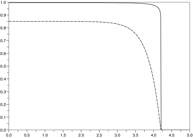
Figure 3: Traveling wave. A traveling wave solution to the mechanical model (1.1), (1.3) in one dimension with $m=40$. The upper continuous line is $\varrho$; the bottom dashed line is $p$. Here $p_{M}=.85$.

A typical application of the Hele-Shaw equations is to describe tumor spheroids [11, 12, 13, 18, 24, 26, 36]. When nutrients are ignored, the tumor is assumed to fill a ball centered at $0$,

$$\Omega(t):=\{p_{\infty}(t)>0\}=\{\varrho_{\infty}(t)=1\}=B_{R(t)}(0).$$

The radius $R(t)$ of this ball is computed according to the geometric motion rules (2.9) and (2.10); that is, we consider the unique (and thus radially symmetric) solution to

(A.1) $$-\Delta p_{\infty}(t)=\Phi(p_{\infty}(t))\quad\text{in }B_{R(t)}(0),\quad\qquad p_{\infty}(R(t),t)=0,$$

and evolve the radius according to

(A.2) $$R^{\prime}(t)=V=|\nabla p_{\infty}(R(t),t)|.$$

Then, we consider $\varrho_{\infty}$ defined as

(A.3) $$\varrho_{\infty}(t)=\mathds{1}_{B_{R(t)}(0)}.$$

This is indeed a correct solution to our model.

Theorem A.1

Let $R(0)=R^{0}$ be given. Problem (A.1)–(A.3) defines a unique dynamic $R(t)$, $\varrho_{\infty}(t)$, $p_{\infty}(t)$, which turns out to be the unique solution to the Hele-Shaw limit problem (2.3) with initial data $\varrho_{\infty}^{0}=\mathds{1}_{B_{R^{0}}(0)}$. For long times it approaches a ‘traveling wave’ solution with a limiting speed independent of the dimension,

(A.4) $$R^{\prime}(t)\underset{t\to\infty}{\longrightarrow}\sqrt{2Q(p_{M})},\qquad Q(p)=\int_{0}^{p}\Phi(q)dq.$$

The limit profile can also be calculated and is one-dimensional.

For several more elaborate one dimensional models, it is also possible to compute the traveling waves which define the asymptotic shape for large times; see [41].

Proof. Existence. A unique solution to (A.1) can be defined for every fixed $R(t)$, because the elliptic problem (A.1) comes with a decreasing nonlinearity. Indeed, shooting or iterative methods apply and give a solution with smooth dependency on the parameter $R(t)$. Therefore the differential equation (A.2) can be solved thanks to the Cauchy-Lipschitz theorem.

Equivalence with the Hele-Shaw problem. To show that this geometric method gives the solution to (2.3), we compute, in the distributional sense, that

$$\partial_{t}\varrho_{\infty}=R^{\prime}(t)\delta_{\partial\Omega(t)}.$$

Also, because $p_{\infty}$ satisfies $\Delta p_{\infty}=\Phi(p_{\infty})$ in $\Omega(t)$ and since $p_{\infty}$ vanishes out of $\Omega(t)$, we have, still in the distributional sense in ${\mathbb{R}}^{N}$, with $\nu$ the unit outward normal to $\Omega(t)$,

$$\Delta p_{\infty}+\varrho_{\infty}\Phi(p_{\infty})=-\delta_{\partial\Omega(t)}\partial_{\nu}p_{\infty}=-\delta_{\partial\Omega(t)}|\nabla p_{\infty}(R(t),t)|,$$

and the last inequality follows from the Dirichlet boundary condition. This means that both formulations, geometric motion of the domain or equation (2.3), are indeed equivalent.

Asymptotic behavior. We use the notation $p_{R}(|x|/R,t):=p_{\infty}(x,t)$. Now $p_{R}$ is solved on the unit ball as

(A.5) $$-p_{R}^{\prime\prime}(r)-\frac{N-1}{r}p_{R}^{\prime}(r)=R^{2}\Phi(p_{R}(r))\quad\mbox{ for }\ 0<r<1,\qquad p_{R}(1)=0,\quad p_{R}^{\prime}(0)=0.$$

By the comparison principle, $p_{R}$ is increasing in $R$ and $p_{R}\leq p_{M}$. Passing to the limit in the equation we find that $p_{R}\to p_{M}$ as $R\to\infty$. It is easy to see that $p_{R}^{\prime}(1)=O(R)$, because we can build sub- and supersolutions of the form $\bar{p}(r)=p_{M}\left(1-\frac{\textrm{e}^{\lambda r}}{\textrm{e}^{\lambda}}\right)$ with $\lambda=CR$ for appropriate values of $C$. By elliptic regularity we conclude that $\|p_{R}^{\prime}\|_{L^{\infty}(\mathbb{R}\times(0,T))}$ is of order $O(R)$ and, since $p_{R}^{\prime}\leq 0$, it is bounded in $L^{1}(\mathbb{R}\times(0,T))$. As a consequence, $\|p_{R}^{\prime}\|_{L^{2}(\mathbb{R}\times(0,T))}$ is of order $O(\sqrt{R})$.

Next we multiply equation (A.5) by $p_{R}^{\prime}$ and integrate in $(0,1)$ to obtain

$$\frac{1}{2}\left(p_{R}^{\prime}(1)\right)^{2}+(N-1)\int_{0}^{1}\frac{\left(p_{R}^{\prime}(r)\right)^{2}}{r}\,dr=R^{2}Q(p_{R}(0))\approx R^{2}Q(p_{M}).$$

From the above $L^{2}$ estimate on $p_{R}^{\prime}$, we conclude that $p_{R}^{\prime}(1)\approx R\sqrt{2Q(p_{M})}$. Going back to the dimensionalized variable, (A.4) follows.

One-dimensional profile. We consider moving coordinates, $s=r-R(t)$, $\hat{p}_{t}(s)=p_{\infty}(s+R(t),t)$. Then $\hat{p}_{t}(s)$ is positive if and only if $s<0$. Hence,

$$\hat{p}_{t}^{\prime\prime}(s)+\frac{N-1}{s-R(t)}p_{t}^{\prime}(s)+\Phi(p_{t}(s))=0\quad\text{for }s<0,\qquad\hat{p}_{t}^{\prime}(0)=-R^{\prime}(t).$$

Since $R(t)\to\infty$ as $t\to\infty$, we can pass to the limit uniformly on compact sets $-K\leq s\leq 0$ to obtain

$$\hat{p}_{\infty}^{\prime\prime}(s)+\Phi(p_{\infty}(s))\quad\text{for }s<0,\qquad\hat{p}_{\infty}^{\prime}(0)=-\sqrt{2Q(p_{M})}.$$

$\square$

Remark. The asymptotic growth rate (A.4) is generic for solutions to (2.3), since one can always sandwich, after a certain delay, any “standard” initial data between two particular profiles of the form (A.3) which asymptotically travel with the same speed (A.4).

A.2 Examples with strong time discontinuities for the pressure

Here we produce examples of solutions with a jump discontinuity in the pressure as a function of time.

The first and simplest example is constructed in radial symmetry. It consists of an initial datum which is constant $c_{0}<1$ in a ball centered at $0$ and of radius 1 and zero otherwise. Then the solution will have 0 pressure for a certain time, $0<t<t_{1}$, in which the density grows exponentially according to equation (2.3), so that

$$\varrho_{\infty}(x,t)=c_{0}\textrm{e}^{\Phi(0)t}\mathds{1}_{B_{1}(0)}.$$

At $t=t_{1}=-\frac{\log c_{0}}{\Phi(0)}$, $\varrho_{\infty}$ reaches the threshold level $\varrho_{\infty}=1$ in $B_{1}$. It cannot happen that $p_{\infty}(t)=0$ for $t>t_{1}$, since otherwise $\varrho_{\infty}$ would violate the bound $\varrho_{\infty}\leq 1$. Therefore, $p_{\infty}(t)$ satisfies $\Delta p_{\infty}+\Phi(p_{\infty})=0$ in some ball $B_{R(t)}$ with $R(t)>0$. An easy argument using the maximum principle shows that $R(t)\geq 1$. It means that $p_{\infty}(t)$ is equal or larger than the solution $\bar{p}_{\infty}$ of the problem $\Delta\bar{p}_{\infty}+\Phi(\bar{p}_{\infty})=0$, $\bar{p}_{\infty}=0$ for $|x|=1$, $\bar{p}_{\infty}>0$ for $|x|<1$. Taking the limit $t\downarrow t_{1}$, we obtain a jump discontinuity in time at $t=t_{1}$ for every $|x|<1$. Note that $p_{\infty}(t)$ is a discontinuous function of time with values in any $L^{p}(\mathbb{R}^{N})$, $p\geq 1$.

The second example is best presented in one space dimension and consists of the evolution of an initial data consisting of two copies of the standard example presented in section A.1 (tumor spheroid), which have now an interval as support. We locate the supports at a distance from each other of say 1. For a time interval, $0<t<t_{1}$ they evolve independently. At $t=t_{1}$, the supports meet and an easy application of the maximum principle, shows that the solution is strictly positive in the union of the two intervals, therefore, larger than the solution corresponding to the union of the two intervals at $t=t_{1}$. An easy inspection of the solutions at times $t_{1}^{-}$ and $t_{1}^{+}$ shows that there is a jump discontinuity in the space pressure profiles. This example can be adapted to several space dimensions by replacing disjoint intervals by disjoint concentric annuli.

A.3 The effect of the equation on $\varrho_{\infty}$

We consider the cell density (defined for short enough times) with two discontinuities

$$\varrho_{\infty}(t)=(1-q(t))\mathds{1}_{B_{R_{1}(t)}}+q(t)\mathds{1}_{B_{R_{2}}},\qquad R_{1}(t)<R_{2},\quad q(t)\leq 1.$$

We claim that the correct dynamics is defined by the speed and values of $q(t)$ given through

$$R_{1}^{\prime}(t)=\frac{1}{1-q(t)}|\nabla p_{\infty}(R_{1}(t),t)|,\qquad q^{\prime}(t)=q(t)\Phi(0)\quad\text{while }q(t)\leq 1,$$

with $p_{\infty}$ vanishing outside the ball of radius $R_{1}(t)$ and satisfying $-\Delta p_{\infty}=\Phi(p_{\infty})$ in $B_{R_{1}(t)}$, with zero Dirichlet boundary condition.

These rules are simply derived from equation (2.3). For $R_{1}(t)<|x|<R_{2}$ we have $p_{\infty}=0$ and thus the equation (2.3) is reduced to $\partial_{t}\varrho_{\infty}(t)=\Phi(0)\varrho_{\infty}(t)$ which gives us the evolution of $q(t)$. For $|x|\leq R_{1}(t)$, we have $\partial_{t}\varrho_{\infty}=R_{1}^{\prime}(t)(1-q(t))\delta_{\{|x|=R_{1}(t)\}}$, while $\Delta p_{\infty}+\varrho_{\infty}\Phi(p_{\infty})=|\nabla p_{\infty}|\delta_{\{|x|=R_{1}(t)\}}$. Using the equation (2.3), we get the dynamics for $R_{1}(t)$.

Acknowledgments. Authors FQ and JLV partially supported by Spanish project MTM2011-24696. The paper was started while they where visiting UPMC. They are indebted to this institution for the warm hospitality. BP is supported by Institut Universitaire de France.

References

- [1] Aronson, D. G.; Bénilan, Ph. Régularité des solutions de l’équation des milieux poreux dans . C. R. Acad. Sci. Paris Sér. A-B 288 (1979), no. 2, A103–A105.
- [2] Aronson, D. G.; Gil, O.; Vázquez, J. L. Limit behaviour of focusing solutions to nonlinear diffusions. Comm. Partial Differential Equations 23 (1998), no. 1-2, 307–332.
- [3] Bellomo, N.; Li, N. K.; Maini, P. K. On the foundations of cancer modelling: selected topics, speculations, and perspectives. Math. Models Methods Appl. Sci. 18 (2008), no. 4, 593–646.
- [4] Bellomo, N.; Preziosi, L. Modelling and mathematical problems related to tumor evolution and its interaction with the immune system. Math. Comput. Modelling 32 (2000), no. 3-4, 413–542.
- [5] Bénilan, Ph.; Boccardo, L.; Herrero, M. A. On the limit of solutions of as . Rend. Sem. Mat. Univ. Politec. Torino. Fascicolo Speciale (1989), 1–13.
- [6] Bénilan, Ph.; Crandall, M. G. The continuous dependence on of solutions of . Indiana Univ. Math. J. 30 (1981), no. 2, 161–177.
- [7] Bénilan, Ph.; Crandall, M. G.; Pierre, M. Solutions of the porous medium equation in under optimal conditions on the initial values. Indiana Univ. Math. J. 33 (1984), no. 1, 51–87.
- [8] Bénilan, Ph.; Igbida, N. Singular limit of perturbed nonlinear semigroups. Comm. Appl. Nonlinear Anal. 3 (1996), no. 4, 23–42.
- [9] Bénilan, Ph.; Igbida, N. La limite de la solution de lorsque . C. R. Acad. Sci. Paris Sér. I Math. 321 (1995), no. 10, 1323–1328.
- [10] Blank, I. A.; Korten, M. K.; Moore, C. N. The Hele-Shaw problem as a “mesa” limit of Stefan problems: existence, uniqueness, and regularity of the free boundary. Trans. Amer. Math. Soc. 361 (2009), no. 3, 1241–1268.
- [11] Brú, A.; Albertos, S.; Subiza, J. L.; Asenjo, J. A.; Brœ, I. The universal dynamics of tumor growth. Biophys. J. 85 (2003), no. 5, 2948–2961.
- [12] Byrne, H. M.; Chaplain, M. A. Growth of necrotic tumors in the presence and absence of inhibitors. Math. Biosci. 135 (1996), no. 15, 187–216.
- [13] Byrne, H. M.; Drasdo, D. Individual-based and continuum models of growing cell populations: a comparison. J. Math. Biol. 58 (2009), no. 4-5, 657–687.
- [14] Byrne, H. M.; Preziosi, L. Modelling solid tumour growth using the theory of mixtures. Math. Med. Biol. 20 (2003), no. 4, 341–366.
- [15] Chaplain, M. A. J. Avascular growth, angiogenesis and vascular growth in solid tumours: the mathematical modeling of the stages of tumor development. Math. Comput. Modeling 23 (1996), no. 6, 47–87.
- [16] Cheng, C. H. A.; Coutand, D.; Shkoller, S. Global existence and decay for solutions of the Hele-shaw flow with injection. Preprint 2012, arXiv:1208.6213 [math.AP].
- [17] Crowley, A. B. On the weak solution of moving boundary problems. J. Inst. Math. Appl. 24 (1979), no. 1, 43–57.
- [18] Cui, S.; Escher, J. Asymptotic behaviour of solutions of a multidimensional moving boundary problem modeling tumor growth. Comm. Partial Differential Equations 33 (2008), no. 4–6, 636–655.
- [19] Cui, S.; Friedman, A. Formation of necrotic cores in the growth of tumors: analytic results. Acta Mat. Sci. 26 (2006), 781–796.
- [20] Di Benedetto, E.; Friedman, A. The ill-posed Hele-Shaw model and the Stefan problem for supercooled water. Trans Amer. Math. Soc. 282 (1984), no. 1, 183–204.
- [21] Egly, H.; Després, B.; Sentis, R. Ablative Hele-Shaw model for ICF flows modeling and numerical simulation. Math. Models Methods Appl. Sci. 21 (2011) no. 7, 1571–1600.
- [22] Elliot, C. M.; Herrero, M. A.; King, J. R.; Ockendon, J. R. The mesa problem: diffusion patterns for as . IMA J. Appl. Math. 37 (1986), no. 2, 147–154.
- [23] Elliot, C. M.; Janovsky, V. A variational inequality approach to Hele-Shaw flow with a moving boundary. Proc. Roy. Soc. Edinburgh. Sect. A 88 (1981), no. 1-2, 93–107.
- [24] Friedman, A. A hierarchy of cancer models and their mathematical challenges. Mathematical models in cancer (Nashville, TN, 2002). Discrete Contin. Dyn. Syst. Ser. B 4 (2004), no. 1, 147–159.
- [25] Friedman, A.; Höllig, K. On the mesa problem. J. Math. Anal. Appl. 123 (1987), no. 2, 564–571.
- [26] Friedman, A.; Hu, B. Stability and instability of Liapunov-Schmidt and Hopf bifurcation for a free boundary problem arising in a tumor model. Trans. Am. Math. Soc. 360 (2008), no. 10, 5291–5342.
- [27] Friedman, A.; Huang, S. Y. Asymptotic behavior of solutions of as with inconsistent initial values. In “Analyse Mathématique et applications”, pp. 165–180, Gauthier-Villars, Paris, 1988.
- [28] Gil, O.; Quirós, F. Convergence of the porous media equation to Hele-Shaw. Nonlinear Anal. Ser. A: Theory Methods 44 (2001), no. 8, 1111–1131.
- [29] Gil, O.; Quirós, F. Boundary layer formation in the transition from the porous media equation to a Hele-Shaw flow. Ann. Inst. H. Poincaré Anal. Non Linéaire 20 (2003), no. 1, 13–36.
- [30] Gil, O.; Quirós, F.; Vázquez, J. L., Zero specific heat limit and large time asymptotics for the one-phase Stefan problem. Preprint.
- [31] Greenspan, H. P. Models for the growth of a solid tumor by diffusion. Stud. Appl. Math. 51 (1972), no. 4, 317–340.
- [32] Igbida, N. The mesa-limit of the porous medium equation and the Hele-Shaw problem. Differential Integral Equations 15 (2002), no. 2, 129–146.
- [33] Jakobsen, E. R.; Karlsen, K. H. Continuous dependence estimates for viscosity solutions of fully nonlinear degenerate parabolic equations. J. Differential Equations 183 (2002), no. 2, 497–525.
- [34] Kim, I. C. Uniqueness and existence results on viscosity solutions of the Hele-Shaw and the Stefan problems. Arch. Rat. Mech. Anal. 168 (2003), no. 4, 299–328.
- [35] Kim, I. C.; Mellet, A. Homogenization of a Hele-Shaw problem in periodic and random media. Arch. Ration. Mech. Anal. 194 (2009), no. 2, 507–530.
- [36] Lowengrub, J. S.; Frieboes H. B.; Jin, F.; Chuang, Y.-L.; Li, X.; Macklin, P.; Wise, S. M.; Cristini, V. Nonlinear modelling of cancer: bridging the gap between cells and tumours. Nonlinearity 23 (2010), no. 1, R1–R91.
- [37] Preziosi, L.; Tosin, A. Multiphase modelling of tumour growth and extracellular matrix interaction: mathematical tools and applications. J. Math. Biol. 58 (2009), no. 4-5, 625–656.
- [38] Ranft, J.; Basana, M.; Elgeti, J.; Joanny, J.-F.; Prost, J.; Jülicher, F. Fluidization of tissues by cell division and apoptosis. Proc. Natl. Acad. Sci. USA (2010), no. 49, 20863–20868.
- [39] Sacks, P. E. A singular limit problem for the porous medium equation. J. Math. Anal. Appl. 140 (1989), no. 2, 456–466.
- [40] Serfaty, S.; Vázquez, J. L. A mean field equation as limit of nonlinear diffusions with fractional Laplacian operators. Preprint 2012, arXiv:1205.6322v2 [math.AP].
- [41] Tang, M.; Vauchelet, N.; Cheddadi, I.; Vignon-Clementel, I.; Drasdo, D.; Perthame, B. Composite waves for a cell population system modelling tumor growth and invasion. Chin. Ann. Math. Ser. B 34 (2013), no. 2, 295–318.
- [42] Vázquez, J. L. “The porous medium equation. Mathematical theory”. Oxford Mathematical Monographs. The Clarendon Press, Oxford University Press, Oxford, 2007. ISBN: 978-0-19-856903-9.