Coherence and decoherence in photon spin-qubit entanglement.

Abstract

We study the dynamics of spontaneous generation of coherence and photon spin-qubit entanglement in a $\Lambda$ system with non-degenerate lower levels. The cases of entanglement in frequency only and frequency and polarization are compared and the reduced density matrix and entanglement entropy are analyzed. We explore in detail how which-path information manifest when the energy difference between the qubit states is larger than the linewidth of the excited state suppresses coherence. A framework is provided to describe the dynamics of spontaneous generation of coherence and (ideal) photodetection obtaining the post measurement qubit density matrix. A simple model of photodetection with a quantum eraser to suppress which-path information in the detection measurement is implemented. It is found that such quantum eraser purifies the qubit density matrix after photodetection, our results are in agreement with those reported in recent experiments.

I Introduction

Quantum entanglement has evolved from being a paradoxical aspect of quantum mechanicsepr to becoming a resource for quantum computing and quantum informationbookqiqc ; kimble ; duan with potential for technological breakthroughs in these areasexpt1 ; horodecki ; esentan . Several recent experiments demonstrated photon entanglement with single atoms photatom1 ; photatom2 ; photatom3 , atomic ensemblesensemble , long-distance entanglement between qubitsentdistance ; zoeller1 ; zoeller2 , and tunable ion-photon entanglement in optical cavitiesions1 ; ions2 . Along with atom-photon entanglementphotatom1 ; photatom2 ; photatom3 ; duan , and entanglement in cavity quantum electrodynamicslcavity recent proposals suggested electron spin-photon entanglement in quantum dots as platforms for entanglement between distant spinsdiode . Spin-photon entanglement could be the pathway towards implementation of quantum networks among distant nodeskimble ; zoeller1 ; zoeller2 . Remarkable experiments demonstrated the realization of entanglement between the polarization of a single optical photon and an electronic spin qubit in nitrogen vacancy (NV) centers in diamonddutt and more recently the demonstration of entanglement between a single electron spin and a photon in a quantum dot has been reportedqdotyama ; qdotgao ; qdot . A main paradigm in many of these experiments is that of spontaneous generation of coherencejava ; sham1 ; sham2 in a type-II or $\Lambda$ system, namely a situation in which spontaneous emission from a single excited state via a two-channel decay to degenerate or non-degenerate lower levels results in coherence between these two states. Spontaneous generation of electron spin coherence has also been observed from the radiative decay of charged excitons (trions) in quantum dotsdotdutt .

These experimental efforts are paving the way towards the implementation of atom-photon or spin-photon entanglement as potential platforms for quantum information and quantum computing protocols and networksimamoglu ; kimble ; duan , motivating a theoretical effort seeking a deeper understanding of these processesshabaev ; chen ; sham1 ; mismatch .

Although there have been some recent studies of the dynamics of spontaneously generated coherencesham1 ; sham2 ; mismatch many important aspects merit further investigation.

Our main goal in this article is to provide a more complete theoretical study of the experimental results reported in ref.dutt but that apply more generally to current experiments on spin-qubit-photon entanglementqdotyama ; qdotgao ; qdot from spontaneous generation of coherence as mentioned above. With this aim, we focus on the following aspects: 1) to provide a treatment of the dynamics of spontaneous generation of coherence, entanglement both in frequency and polarization and photodetection within a single framework consistent with causalitycausality , 2) to study the entanglement entropy of reduced spin-qubit density matrices after tracing over the radiation degrees of freedom for photon-qubit entanglement both in frequency and polarization, of particular interest when spontaneous emission produces polarized photons which are measured by projection on differen polarization states 3) to analyze in detail how which- path information affects coherence, in particular within the setting of the experiment in ref.dutt , predicting the time dependence of conditional probabilities when which path information is present. 4)To implement a model for a “quantum eraser”eraser1 ; eraser2 within the framework of photodetection a lá Glauberbook1 ; book2 ; glauber so as to erase which path information in the photodetection process. An important result of this treatment is that “quantum erasing” “which- path” information leads to the purification of the qubit state confirming the experimental results of ref.dutt ; qdotyama and bolstering the arguments on “quantum erasing” in these references. We obtain a conditional probability in complete agreement with the experimental results of ref.dutt .

Our study differs from and complements recent theoretical treatments of spontaneous generation of coherencesham1 ; mismatch in that we analyze both frequency and polarization entanglement, which-path decoherence, the spin-qubit entanglement entropy and incorporate a Glauber model of broadband photodetection[34,35,36] in a unified manner with the treatment of spontaneous emission. This treatment directly builds in causality in the spontaneous emission/photodetection process[31], leads to detailed understanding of how which path information affects coherence, and allows to model a quantum eraser[32,33] consistently within the broadband photodetector model. This approach is different from that advocated in a recent articlemismatch where the photodetector is modeled with a collection of two-state atoms spread over some distance where the excited state features a short lifetime. Furthermore our study also differs from those of refs.sham1 ; mismatch in that it shows how the implementation of a “quantum eraser” leads to the purification of the qubit density matrix upon photodetection and yields a result for the conditional probability in complete agreement with the experimental findings in ref.[19].

II Dynamics of entanglement via spontaneous decay.

We consider a $\Lambda$-system with one excited state $|A\rangle$ and two Zeeman split non-degenerate lower levels interacting with the electromagnetic field in the dipole and rotating wave approximations. The degenerate case can be obtained straightforwardly. We refer to the two-lower state levels $|\pm 1\rangle$ as a spin- qubit. The cases in which there is photon-qubit entanglement in frequency only and in frequency and polarization are studied separately and compared.

II.1 Entanglement in frequency only:

We first consider the case when the dipole matrix elements are independent of the polarization of the photon and for simplicity we only consider one polarization to establish contact with the results of ref.sham1 . This case leads to qubit-photon entanglement in frequency only, and generalization to two polarizations is straightforward. The total Hamiltonian for the three level system is given by

$$H=H_{A}+H_{R}+H_{AR}\,,$$ (II.1)

where

$$H_{A}=E_{A}|A\rangle\langle A|+E_{+}|+1\rangle\langle+1|+E_{-}|-1\rangle\langle-1|~{}~{};~{}~{}H_{R}=\sum_{\vec{k}}\omega_{k}a^{\dagger}_{\vec{k}}a_{\vec{k}}\,.$$ (II.2)

The interaction Hamiltonian in the interaction picture and in the rotating wave approximation is given by

$$H_{AR}(t)=\sum_{\vec{k}}\Bigg{\{}g_{k}\,a^{\dagger}_{\vec{k}}\Big{[}|+1\rangle\langle A|\,e^{i(k-\Omega_{+})t}+|-1\rangle\langle A|\,e^{i(k-\Omega_{-})t}\Big{]}+\mathrm{h.c.}\Bigg{\}}$$ (II.3)

where

$$\Omega_{\pm}=E_{A}-E_{\pm}~{}~{};~{}~{}g_{k}=-i\sqrt{\frac{k}{2V}}~{}{D}\,,$$ (II.4)

here $V$ is the volume and $D$ is the dipole matrix element neglecting polarization degrees of freedom.

Consider that at time $t=0$ the initial state is

$$|\Psi(0)\rangle=|A\rangle\ |0_{\gamma}\rangle$$ (II.5)

where $|0_{\gamma}\rangle$ is the radiation vacuum state, and write in the interaction picture the time evolved state as

$$|\Psi(t)\rangle_{I}=C_{A}(t)|A\rangle|0_{\gamma}\rangle+\sum_{\vec{k}}|1_{\vec{k}}\rangle\Big{[}{C}_{k,+}(t)\,|+1\rangle+{C}_{k,-}(t)\,|-1\rangle\Big{]}\,.$$ (II.6)

The coefficients obey the following equations (in obvious notation)

$$\dot{C}_{A}(t) = -i\langle A;0_{\gamma}|H_{AR}(t)|1_{\vec{k}};+1\rangle\,{C}_{k,+}(t)-i\langle A;0_{\gamma}|H_{AR}(t)|1_{\vec{k}};-1\rangle\,{C}_{k,-}(t)$$ (II.7)

$$\dot{C}_{k,\pm}(t) = -i\langle 1_{\vec{k}};\pm 1|H_{AR}(t)|A;0_{\gamma}\rangle\,{C}_{A}(t)\,.$$ (II.8)

We solve this system of equations with the initial conditions

$$C_{A}(0)=1~{};~{}{C}_{k,\pm}(0)=0\,.$$ (II.9)

In the Wigner-Weisskopf approximationbook1 ; ww the coefficients are given by

$$C_{A}(t) = e^{-\frac{\Gamma}{2}t}\,,$$ (II.10)

$${C}_{k,\pm}(t) = ig_{k}\,~{}\frac{\Big{[}1-e^{i\big{(}k-\Omega_{\pm}+i\Gamma/2\big{)}t}\Big{]}}{\Big{(}k-\Omega_{\pm}+i\frac{\Gamma}{2}\Big{)}}\,.$$ (II.11)

The level width $\Gamma$ is given by

$$\Gamma=\Gamma_{+}+\Gamma_{-}$$ (II.12)

where the partial widths $\Gamma_{\pm}$ correspond to the spontaneous decay channels $|A;0_{\gamma}\rangle\rightarrow|1_{\vec{k}}\rangle|+1\rangle;|A\rangle\rightarrow|1_{\vec{k}}\rangle|-1\rangle$ respectively, namely

$$\Gamma_{\pm}=2\pi\,\sum_{\vec{k}}|\langle A|H_{AR}(0)|1_{\vec{k}};\pm 1\rangle|^{2}\,\delta(k-\Omega_{\pm})=2\pi\,\sum_{\vec{k}}|g_{k}|^{2}\,\delta(k-\Omega_{\pm})=\frac{D^{2}\Omega^{3}_{\pm}}{2\pi}$$ (II.13)

In most experimental circumstances, the energy splitting is much smaller than the optical frequency of the transitions, namely $|\Omega_{+}-\Omega_{-}|\ll\Omega_{\pm}$ in which case it is convenient to write

$$\Omega_{\pm}=\Omega\pm\frac{\Delta\omega}{2}~{}~{};~{}~{}\Delta\omega\ll\Omega$$ (II.14)

and to leading order in $\Delta\omega/\Omega$ it follows that

$$\Gamma_{+}\simeq\Gamma_{-}\simeq\Gamma/2\,.$$ (II.15)

In the experiment reported in ref.dutt , it has been verified that the approximation (II.15) is fulfilled in the setting of that experiment. In what follows we will assume that the relation (II.15) holds unless otherwise stated.

We write the spin qubit-photon entangled part of the wavefunction (in the interaction picture) (II.6) as

$$|\Psi_{sp}(t)\rangle=\frac{1}{\sqrt{2}}\Big{[}|\sigma_{1}(t)\rangle|+1\rangle+|\sigma_{2}(t)\rangle|-1\rangle\Big{]}$$ (II.16)

where the single photon wavepackets are given by

$$|\sigma_{1}(t)\rangle=\sqrt{2}\sum_{\vec{k}}{C}_{k,+}(t)|1_{\vec{k}}\rangle~{}~{};~{}~{}|\sigma_{2}(t)\rangle=\sqrt{2}\sum_{\vec{k}}{C}_{k,-}(t)|1_{\vec{k}}\rangle$$ (II.17)

II.2 Normalization of photon wavepackets:

The normalization and orthogonality of the single photon wave-packets is determined by the overlaps

$$\langle\sigma_{a}(t)|\sigma_{b}(t)\rangle=2\sum_{\vec{k}}{C}_{\vec{k},b}(t)\,{C}^{*}_{\vec{k},a}(t)~{}~{};~{}~{}a,b=1,2\,.$$ (II.18)

Consider the functions

$$\mathcal{G}_{\alpha}(\omega,t)=\frac{\Big{[}1-e^{i(\omega-\Omega_{\alpha}+i\frac{\Gamma}{2})t}\Big{]}}{\Big{[}\omega-\Omega_{\alpha}+i\,\frac{\Gamma}{2}\Big{]}}\,$$ (II.19)

in the narrow width limit $\Gamma\ll\Omega_{\alpha}$ these are sharply localized near $\omega\simeq\Omega_{\alpha}$, straightforward contour integration yields

$$\int_{-\infty}^{\infty}\mathcal{G}_{\alpha}(\omega,t)\mathcal{G}^{*}_{\beta}(\omega,t)\,d\omega=2\pi\,\frac{\Big{[}1-e^{-i(\Omega_{\alpha}-\Omega_{\beta})t}\,e^{-\Gamma t}\Big{]}}{\Gamma+i(\Omega_{\alpha}-\Omega_{\beta})}\,.$$ (II.20)

Combining this result with (II.17,II.11) we find consistently with the Wigner-Weisskopf approximation

$$\langle\sigma_{1,2}(t)|\sigma_{1,2}(t)\rangle=\frac{2\Gamma_{+,-}}{\Gamma}\Big{[}1-e^{-\Gamma t}\Big{]}\,.$$ (II.21)

This result, along with the relation between the total and partial decay widths given by (II.12) yields the normalization of the $|\Psi_{sp}\rangle$ state,

$$\langle\Psi_{sp}(t)|\Psi_{sp}(t)\rangle=\Big{[}1-e^{-\Gamma t}\Big{]}\,,$$ (II.22)

which is a result of unitary time evolution manifest in the Weisskopf-Wigner formulation since the total state $|\Psi(t)\rangle_{I}$ given by (II.6) must obey $\langle\Psi(t)|\Psi(t)\rangle=1$. Because $|\sigma_{1,2}\rangle$ are single photon wavepackets, it is straightforward to confirm that the total number of photons is given by

$$N_{\gamma}(t)=\langle\Psi_{sp}(t)\Big{|}\sum_{\vec{k}}a^{\dagger}_{\vec{k}}a_{\vec{k}}\Big{|}\Psi_{sp}(t)\rangle=\Big{[}1-e^{-\Gamma t}\Big{]}\,.$$ (II.23)

Taking $\Gamma_{+}\simeq\Gamma_{-}\simeq\Gamma/2$ under the assumption that $\Delta\omega\ll\Omega$, consistent with the experimental setup in dutt , it follows that the single photon wavepackets are normalized for $\Gamma t\gg 1$ but they are not orthogonal, we find

$$\langle\sigma_{2}(t)|\sigma_{1}(t)\rangle=\frac{\Big{[}1-e^{-i\Delta\omega t}\,e^{-\Gamma t}\Big{]}}{1+i\frac{\Delta\omega}{\Gamma}}\,,$$ (II.24)

a result that is in agreement with an observation in ref.sham1 for $\Gamma t\gg 1$.

Let us consider the reduced density matrix for the qubit by tracing over the radiation field, namely (in the interaction picture)

$$\rho^{I}_{fo}(t)=\mathrm{Tr}_{R}|\Psi_{sp}(t)\rangle\langle\Psi_{sp}(t)|\,,$$ (II.25)

going back to the Schroedinger picture we find

$$\rho_{fo}(t)=\frac{1}{2}\Big{[}1-e^{-\Gamma t}\Big{]}\Bigg{\{}|+1\rangle\langle+1|+|-1\rangle\langle-1|+\Bigg{(}e^{i\Delta\omega t}\,\eta(t)\,|+1\rangle\langle-1|+\mathrm{h.c.}\Bigg{)}\Bigg{\}}$$ (II.26)

where

$$\eta(t)\equiv|\eta(t)|e^{i\varphi(t)}=\frac{\,\Big{[}1-e^{-i\Delta\omega\,t}~{}e^{-\Gamma t}\Big{]}}{\big{(}1-e^{-\Gamma t}\big{)}\big{(}1+i\frac{\Delta\omega}{\Gamma}\big{)}}\,.$$ (II.27)

In the long time limit $\Gamma t\gg 1$ the coherence is suppressed by the factor $1/\sqrt{1+\Delta\omega^{2}/\Gamma^{2}}$ reflecting the suppression of coherence by “which-path” information. If $\Gamma\gg\Delta\omega$ the spectral width of the radiation, determined by the lifetime of the excited state, suppresses which path information by blurring the energy resolution of the decay channels of the emitted photons and coherence is maintained. In the opposite limit $\Delta\omega\gg\Gamma$ the energy difference between the lower lying states is resolved and which path information is available in the emission spectrum thereby suppressing coherence. This is manifest in the overlap of the photon wavepackets (II.24) in terms of the product of the Lorentzian line shapes for the individual channels.

The main reason for studying the reduced density matrix in the case of frequency entanglement only is that, as it will be discussed in detail in section (III) photodetection that filters horizontal (H) or vertically (V) polarized photons projects the density matrix onto a reduced density matrix precisely of the form (II.26) that contains “which-path” information.

II.3 Entanglement in frequency and polarization

In the experimental situations considered in refs.photatom1 ; photatom2 ; photatom3 for atom-photon entanglement and in ref.dutt for electron spin-photon entanglement in NV-centers, there are angular momentum selection rules in spontaneous decay and the photons emitted are right handed (for $|A\rangle\rightarrow|-1\rangle$) or left handed (for $|A\rangle\rightarrow|+1\rangle$) circularly polarized as depicted in fig. (1). In this case the spin- qubit and the spontaneously emitted photons are entangled both in polarization and frequency. Including the polarization of the emitted photons leads to several important modifications of the results obtained in the previous case, therefore we restore the polarization, momentum and spatial dependence of the dipole matrix elements. Although we focus the discussion on the experimental setup of ref.dutt with NV-centers, the results will be more general.

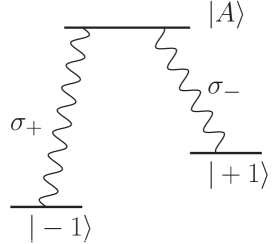
Figure 1: Transitions

In this case the total Hamiltonian for the three level $\Lambda$-system interacting with the electromagnetic field is given by (II.1) with $H_{A}$ given in eqn. (II.2), but now

$$H_{R}=\sum_{\vec{k},\lambda=\pm}\omega_{k}a^{\dagger}_{\vec{k},\lambda}a_{\vec{k},\lambda}\,,$$ (II.28)

and the interaction Hamiltonian in the interaction picture and in the rotating wave approximation is given by

$$H_{AR}(t)=\sum_{\vec{k}}\Bigg{\{}g_{\vec{k},+}(\vec{x}_{0})\,a^{\dagger}_{\vec{k},-}|+1\rangle\langle A|\,e^{i(k-\Omega_{+})t}+g_{\vec{k},-}(\vec{x}_{0})\,a^{\dagger}_{\vec{k},+}|-1\rangle\langle A|\,e^{i(k-\Omega_{-})t}+\mathrm{h.c.}\Bigg{\}}$$ (II.29)

where $\Omega_{\pm}=E_{A}-E_{\pm}$, and

$$g_{\vec{k},\pm}(\vec{x}_{0})=-i\sqrt{\frac{k}{2V}}\,\vec{D}_{\pm}\cdot\vec{\epsilon}_{\vec{k},\mp}\,e^{i\vec{k}\cdot\vec{x}_{0}}$$ (II.30)

here $V$ is the volume, $\vec{D}_{\pm}$ are the dipole matrix elements $\langle\pm 1|\vec{d}|A\rangle$ respectively, $\vec{\epsilon}_{\vec{k},\mp}$ are the left and right handed polarization vectors respectively and $\vec{x}_{0}$ is the position of the NV center.

Consider that at time $t=0$ the initial state is

$$|\Psi(0)\rangle=|A\rangle\ |0_{\gamma}\rangle$$ (II.31)

where $|0_{\gamma}\rangle$ is the radiation vacuum state, and following the notation of the previous section we write the time evolved state in the interaction picture as

$$|\Psi(t)\rangle_{I}=C_{A}(t)|A\rangle|0_{\gamma}\rangle+\sum_{\vec{k}}\Bigg{[}{C}_{\vec{k},+}(t)\,|1_{\vec{k},-}\rangle|+1\rangle+{C}_{\vec{k},-}(t)\,|1_{\vec{k},+}\rangle|-1\rangle\Bigg{]}\,.$$ (II.32)

The coefficients obey the following equations (in obvious notation)

$$\dot{C}_{A}(t) = -i\langle A;0_{\gamma}|H_{AR}(t)|1_{\vec{k},+};-1\rangle\,{C}_{\vec{k},-}(t)-i\langle A;0_{\gamma}|H_{AR}(t)|1_{\vec{k},-};+1\rangle\,{C}_{\vec{k},+}(t)$$ (II.33)

$$\dot{C}_{\vec{k},\pm}(t) = -i\langle 1_{\vec{k},\mp};\pm 1|H_{AR}(t)|A;0_{\gamma}\rangle\,{C}_{A}(t)\,.$$ (II.34)

Just as in the previous section we solve this system of equations with the initial conditions $C_{A}(0)=1~{};~{}{C}_{\vec{k},\pm}(0)=0$, in the Wigner-Weisskopf approximation the coefficients are given by

$$C_{A}(t) = e^{-\frac{\Gamma}{2}\,t}\,,$$ (II.35)

$${C}_{\vec{k},\pm}(t) = ig_{\vec{k},\pm}(\vec{x}_{0})\,~{}\frac{\Big{[}1-e^{i\big{(}k-\Omega_{\pm}+i\Gamma/2\big{)}t}\Big{]}}{\Big{(}k-\Omega_{\pm}+i\frac{\Gamma}{2}\Big{)}}\,.$$ (II.36)

The level width $\Gamma$ is given by

$$\Gamma=\Gamma_{+}+\Gamma_{-}$$ (II.37)

where the partial widths $\Gamma_{+}\,,\,\Gamma_{-}$ correspond to the spontaneous decay channels $|A;0_{\gamma}\rangle\rightarrow|1_{\vec{k},+}\rangle|-1\rangle;|A\rangle\rightarrow|1_{\vec{k},-}\rangle|+1\rangle$ respectively, namely

$$\Gamma_{+}=2\pi\,\sum_{\vec{k}}|\langle A|H_{AR}(0)|1_{\vec{k},-};+1\rangle|^{2}\,\delta(k-\Omega_{+})=2\pi\,\sum_{\vec{k}}|g_{\vec{k},+}(\vec{x}_{0})|^{2}\,\delta(k-\Omega_{+})$$ (II.38)

$$\Gamma_{-}=2\pi\,\sum_{\vec{k}}|\langle A|H_{AR}(0)|1_{\vec{k},+};+1\rangle|^{2}\,\delta(k-\Omega_{-})=2\pi\,\sum_{\vec{k}}|g_{\vec{k},-}(\vec{x}_{0})|^{2}\,\delta(k-\Omega_{-})\,.$$ (II.39)

Just as in the previous case of unpolarized photons, it follows that $\Gamma_{\pm}\propto|\vec{D}_{\pm}|^{2}\,\Omega^{3}_{\pm}$ but the proportionality constants now depend on the angular average of the polarization vectors.

Now the second term of the wave function (II.32) describes an entangled state of circularly polarized photons and the spin states of the NV- center, following the literaturephotatom1 ; photatom2 ; photatom3 ; dutt we write this second term (in the interaction picture) as

$$|\Psi_{sp}(t)\rangle=\frac{1}{\sqrt{2}}\Big{[}|\sigma_{-}(t)\rangle\,|+1\rangle+|\sigma_{+}(t)\rangle\,|-1\rangle\Big{]}$$ (II.40)

where

$$|\sigma_{\mp}(t)\rangle=\sqrt{2}\,\sum_{\vec{k}}{C}_{\vec{k},\pm}(t)\,|1_{\vec{k},\mp}\rangle$$ (II.41)

describe orthogonal circularly polarized single photon wave packets.

Unlike the results in ref.sham1 we do not take the limit $\Gamma t\gg 1$, in the experimental setting of ref.dutt the lifetime of the excited state is $1/\Gamma\approx 12\,\mathrm{ns}$ but the measurements are performed during a time interval $\simeq 10-20\,\mathrm{ns}$.

Borrowing the results from the previous section, we now find

$$\langle\sigma_{\mp}(t)|\sigma_{\mp}(t)\rangle=\frac{2\,\Gamma_{\pm}}{\Gamma}\Big{[}1-e^{-\Gamma t}\Big{]}~{}~{};~{}~{}\langle\sigma_{+}(t)|\sigma_{-}(t)\rangle=0\,,$$ (II.42)

where the orthogonality of $|\sigma_{\mp}(t)\rangle$ is a consequence of the fact that they describe one photon wavepackets with orthogonal polarizations. This result, along with the relation between the total and partial decay widths given by (II.37) again yields the normalization of the $|\Psi_{sp}\rangle$ state,

$$\langle\Psi_{sp}(t)|\Psi_{sp}(t)\rangle=\Big{[}1-e^{-\Gamma t}\Big{]}\,,$$ (II.43)

which is a result of unitary time evolution and similarly

$$N_{\gamma}(t)=\langle\Psi_{sp}(t)\Big{|}\sum_{\vec{k},\lambda=\pm}a^{\dagger}_{\vec{k},\lambda}a_{\vec{k},\lambda}\Big{|}\Psi_{sp}(t)\rangle=\Big{[}1-e^{-\Gamma t}\Big{]}\,.$$ (II.44)

Just as in the previous section the one-photon wave packets $|\sigma_{\pm}\rangle$ have unit normalization when $\Gamma t\gg 1$ and $\Gamma_{+}=\Gamma_{-}=\Gamma/2$, which is justified when the Zeeman splitting $\Omega_{+}-\Omega_{-}\ll\Omega_{+},\Omega_{-}$ and describes the experimental setup of ref.dutt . The reduced density matrix for the spin-qubit can be obtained by tracing over the radiation field just as in the previous section (II.25,II.26). However, in this case, the orthogonality of the circularly polarized wave packets leads to vanishing coherence and a diagonal density matrix that describes a statistical mixture given by

$$\rho_{fp}(t)=\mathrm{Tr}|\Psi_{sp}(t)\rangle\langle\Psi_{sp}(t)|=\frac{1}{2}\Big{[}1-e^{-\Gamma t}\Big{]}\Big{(}|+1\rangle\langle+1|+|-1\rangle\langle-1|\Big{)}\,.$$ (II.45)

II.4 Entanglement entropy:

As we have seen above spontaneous generation of coherence leads to very different reduced density matrices depending on whether photon-qubit entanglement is in frequency and polarization or frequency only. This difference is highlighted by comparing the Von-Neumann entanglement entropy in both cases.

Frequency entanglement only: in this case the total reduced density matrix is

$$\rho(t)=e^{-\Gamma t}|A\rangle\langle A|+\rho_{fo}(t)$$ (II.46)

where $\rho_{fo}(t)$ is given by (II.26) which can be diagonalized with the following eigenvectors and eigenvalues

$$\widetilde{|1\rangle} = \frac{1}{\sqrt{2}}\Big{(}|+1\rangle+e^{-i\varphi(t)}\,e^{-i\Delta\omega t}|-1\rangle\Big{)}~{}~{};~{}~{}\lambda_{1}(t)=\frac{1}{2}\Big{[}1-e^{-\Gamma t}\Big{]}\,\Big{[}1+|\eta(t)|\Big{]}$$ (II.47)

$$\widetilde{|2\rangle} = \frac{1}{\sqrt{2}}\Big{(}|+1\rangle-e^{-i\varphi(t)}\,e^{-i\Delta\omega t}|-1\rangle\Big{)}~{}~{};~{}~{}\lambda_{2}(t)=\frac{1}{2}\Big{[}1-e^{-\Gamma t}\Big{]}\,\Big{[}1-|\eta(t)|\Big{]}\,$$ (II.48)

where $\eta(t)=|\eta(t)|e^{i\varphi(t)}$ is given by (II.27), leading to

$$\rho(t)=e^{-\Gamma t}|A\rangle\langle A|+\lambda_{1}(t)~{}\widetilde{|1\rangle}\widetilde{\langle 1|}+\lambda_{2}(t)~{}\widetilde{|2\rangle}\widetilde{\langle 2|}\,.$$ (II.49)

The entanglement entropy follows directly,

$$S_{fo}(t)=\Gamma te^{-\Gamma t}-\lambda_{1}(t)\ln\lambda_{1}(t)-\lambda_{2}(t)\ln\lambda_{2}(t)\,.$$ (II.50)

For $\Gamma t\gg 1$

$$S_{fo}(\infty)=-\frac{1}{2}\bigg{[}{1+|\eta_{\infty}|}\bigg{]}\,\ln\bigg{[}\frac{1+|\eta_{\infty}|}{2}\bigg{]}-\frac{1}{2}\bigg{[}1-|\eta_{\infty}|\bigg{]}\,\ln\bigg{[}\frac{1-|\eta_{\infty}|}{2}\bigg{]}$$ (II.51)

with

$$|\eta_{\infty}|=\frac{1}{\sqrt{1+\frac{\Delta\omega^{2}}{\Gamma^{2}}}}$$ (II.52)

As $\Delta\omega/\Gamma\rightarrow 0$ the entanglement entropy vanishes as the asymptotic state is the pure state $\widetilde{|1\rangle}=\frac{1}{\sqrt{2}}\Big{(}|+\rangle+|-\rangle\Big{)}$ in the opposite limit $\Delta\omega/\Gamma\gg 1$ where which-path information suppresses coherence it follows that $S_{fo}(\infty)=\ln(2)$ describing an equal probability statistical mixture.

Entanglement in frequency and polarization: in this case the total reduced density matrix is simply

$$\rho(t)=e^{-\Gamma t}|A\rangle\langle A|+\frac{1}{2}\Big{[}1-e^{-\Gamma t}\Big{]}\Big{(}|+1\rangle\langle+1+|-1\rangle\langle-1|\Big{)}\,$$ (II.53)

as a consequence of the orthogonality of the right and left circular polarized photon wavepackets. In this case the entanglement entropy is

$$S_{fp}(t)=\Gamma te^{-\Gamma t}-[1-e^{-\Gamma t}]\ln\Big{[}\frac{1-e^{-\Gamma t}}{2}\Big{]}$$ (II.54)

with the asymptotic value

$$S_{fp}(\infty)=\ln(2)\,.$$ (II.55)

The entanglement entropies in both cases are displayed in fig.(2) for the parameters of the experiment in ref.dutt , $\Delta\omega=2\pi\times 122\,\mathrm{MHz}~{};~{}\Gamma=1/12\,\mathrm{ns}$.

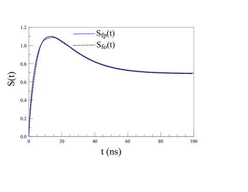
Figure 2: Entanglement entropy for the case of entanglement in frequency only $S_{fo}(t)$ and frequency and polarization $S_{fp}(t)$ for $\Delta\omega=2\pi\times 122\,\mathrm{MHz}~{};~{}\Gamma=1/12\,\mathrm{ns},\Gamma_{+}=\Gamma_{-}=\Gamma/2$.

Analytically it can be seen that

$$S_{fp}(t)\geq S_{fo}(t)\,,$$ (II.56)

a relation that is confirmed numerically and confirms the qualitative expectation that the entanglement entropy should be larger in the case of entanglement both in frequency and polarization.

The results above were obtained under the assumption that $\Gamma_{+}=\Gamma_{-}=\Gamma/2$. If the partial widths to the two non-degenerate levels are different the generalized form of the entanglement entropy in this case of entanglement in frequency and polarization is given by

$$S_{fp}(t)=\Gamma te^{-\Gamma t}-\frac{\Gamma_{+}}{\Gamma}\big{(}1-e^{-\Gamma t}\big{)}\ln\Big{[}\frac{\Gamma_{+}}{\Gamma}\big{(}1-e^{-\Gamma t}\big{)}\Big{]}-\frac{\Gamma_{-}}{\Gamma}\big{(}1-e^{-\Gamma t}\big{)}\ln\Big{[}\frac{\Gamma_{-}}{\Gamma}\big{(}1-e^{-\Gamma t}\big{)}\Big{]}$$ (II.57)

where $\Gamma=\Gamma_{+}+\Gamma_{-}$.

III Photodetection

We consider a model for a broadband photodetector described by an atom localized at position $\vec{x}_{d}$ interacting with the radiation field in the dipole approximation a lá Glauberglauber ; book1 ; book2 . The Hamiltonian is given by $H_{D}+H_{DR}$ where the detector Hamiltonian $H_{D}$ describes a zero energy ground state and a collection of excited states which eventually will be taken as a continuum

$$H_{D}=\nu_{0}\,|g^{d}\rangle\langle g^{d}|+\sum_{j}\nu_{j}|e^{d}_{j}\rangle\langle e^{d}_{j}|~{}~{};~{}~{}\nu_{0}=0\,,$$ (III.1)

and $H_{DR}$ is the interaction Hamiltonian that describes a dipolar coupling to the radiation field with a filter that selects $H/V$ linear polarization states of the radiation field. In the rotating wave approximation and in the interaction picture it is given by

$$H_{DR}(t)=\sum_{j}\Big{[}\vec{d}_{j}\cdot\vec{E}^{(+)}_{P}(\vec{x}_{d};t)|e^{d}_{j}\rangle\langle g^{d}|\,e^{i\nu_{j}t}+\mathrm{h.c.}\Big{]}~{}~{};~{}~{}P=H;V\,$$ (III.2)

$\vec{d}_{j}$ are the dipole matrix elements and

$$\vec{E}^{(+)}_{P}(\vec{x}_{d};t)=\sum_{\vec{k}}i\sqrt{\frac{k}{2V}}~{}\vec{\epsilon}_{P}~{}a_{\vec{k},P}\,e^{i\vec{k}\cdot{\vec{x}_{d}}}e^{-ikt}\,.$$ (III.3)

The combined process of spontaneous emission from the NV-center $|A\rangle$ considered to be localized at $\vec{x}_{0}=\vec{0}$ and photodetection by a broadband photodetector localized at $\vec{x}_{d}$ is now described by the total Hamiltonian

$$H_{tot}=H_{A}+H_{R}+H_{AR}+H_{D}+H_{DR}\,,$$ (III.4)

where the first three terms are given by (II.1-II.3).

Insight into the combined processes and the intermediate states that contribute is gleaned in second order in the perturbative expansion with the full interaction Hamiltonian in the interaction picture (and in the rotating wave approximation)

$$H_{I}(t)=H_{AR}(t)+H_{DR}(t)$$ (III.5)

where $H_{AR}(t);H_{DR}(t)$ are given by (II.29) with $\vec{x}_{0}=\vec{0}$ and (III.2) respectively. Consider that the initial state is (in obvious notation)

$$|\Psi(0)\rangle=|A;0_{\gamma};g^{d}\rangle\,,$$ (III.6)

in the interaction picture the resulting time dependent state in second order becomes

$$|\Psi(t)\rangle=\Bigg{[}1-i\int^{t}_{0}H_{I}(t_{1})dt_{1}+(-i)^{2}\int^{t}_{0}\int^{t_{1}}_{0}H_{I}(t_{1})H_{I}(t_{2})dt_{1}dt_{2}+\cdots\Bigg{]}|\Psi(0)\rangle\,.$$ (III.7)

To first order only $H_{AR}$ contributes and describes the perturbative spontaneous decay of the excited state $|A\rangle$ of the NV-center into the Zeeman split states $|1_{\vec{k},+};-1\rangle$ and $|1_{\vec{k},-};+1\rangle$. Inserting a complete set of eigenstates of $H_{0}=H_{A}+H_{D}+H_{R}$ it is straightforward to see that in the second order contribution the first term $H_{I}(t_{2})$ describes the spontaneous emission of the circularly polarized photons while the second term $H_{I}(t_{1})$ describes the absorption of these photons and the photoexcitation of the detector (along with a second order contribution from $H_{AR}$ that yields the original state back). The photodetection probability at time $t$ is given byglauber ; book1 ; book2

$$P_{D}(t)={\mathrm{Tr}}_{d}\sum_{j}|e^{d}_{j}\rangle\langle e^{d}_{j}|\rho(t)\,,$$ (III.8)

where the density matrix

$$\rho(t)=|\Psi(t)\rangle\langle\Psi(t)|\,,$$ (III.9)

and the trace in (III.8) is over the detector excited states.

Our goal is to describe these processes non-perturbatively with a Wigner-Weisskopf description that incorporates both processes at once. Guided by this perturbative analysis, we propose the following form of the time dependent state in the interaction picture

$$|\Psi(t)\rangle=|\Psi_{A}(t)\rangle\,|g^{d}\rangle+|\Psi_{DS}(t)\rangle\,|0_{\gamma}\rangle$$ (III.10)

where

$$|\Psi_{A}(t)\rangle=C_{A}(t)|A\rangle|0_{\gamma}\rangle+\sum_{\vec{k}}\Bigg{[}{C}_{\vec{k},+}(t)\,|1_{\vec{k},-}\rangle|+1\rangle+{C}_{\vec{k},-}(t)\,|1_{\vec{k},+}\rangle|-1\rangle\Bigg{]}$$ (III.11)

and

$$|\Psi_{DS}(t)\rangle=\sum_{j}\Big{[}D_{j,-}(t)|-1\rangle+D_{j,+}(t)|+1\rangle\Big{]}|e^{d}_{j}\rangle\,,$$ (III.12)

with the initial conditions

$$C_{A}(0)=1~{};~{}C_{\vec{k},\pm}(0)=0~{};~{}D_{j,\pm}(0)=0\,.$$ (III.13)

We highlight that $|\Psi_{DS}(t)\rangle$ describes an entangled state between the spins and the detector.

The explicit solution for the coefficients with the initial conditions (III.13) is provided in the appendix.

The coefficients $D_{j,\pm}(t)$ determine the photodetection probability and display the causal nature of the propagationcausality : the detection time $t_{D}$ has to be larger than $t_{d}=x_{d}/c$, namely the time it takes the front of the photon pulse to travel from the NV-center to the position of the photodetector. In the experimental setup of ref.dutt the photon travels along a $\sim 2\,\mathrm{m}$ long fiber to the photodetector, therefore $t_{d}\simeq 7\,\mathrm{ns}$.

The photodetection probability is obtained as in (III.8), and obviously only the state $|\Psi_{DA}(t)\rangle$ contributes. The result is a projected reduced density matrix for the spin-qubit subpace $|\pm 1\rangle$ namely

$$\rho^{(I)}_{D}(t)={\mathrm{Tr}}_{d}\sum_{j}|e^{d}_{j}\rangle\langle e^{d}_{j}||\Psi_{DS}(t)\rangle\langle\Psi_{DS}(t)|= \sum_{j}\Bigg{[}|D_{j,+}(t)|^{2}~{}|+1\rangle\langle+1|+|D_{j,-}(t)|^{2}~{}|-1\rangle\langle-1|$$

$$+ \Big{(}D_{j,+}(t)D^{*}_{j,-}(t)~{}|+1\rangle\langle-1|+\mathrm{h.c.}\Big{)}\Bigg{]}\,.$$ (III.14)

where the coefficients $D_{j,\pm}(t)$ are given in the appendix by (A.7). We now introduce the density of states of the photodetector $\mathcal{D}(\omega)$: for any arbitrary function of the detector frequencies $\mathcal{F}(\nu_{j})$

$$\sum_{j}|\kappa^{2}_{j}|\,\mathcal{F}(\nu_{j})=\int_{-\infty}^{\infty}\mathcal{D}(\omega)\mathcal{F}(\omega)d\omega~{}~{};~{}~{}\mathcal{D}(\omega)=\sum_{j}|\kappa^{2}_{j}|\delta(\omega-\nu_{j})\,.$$ (III.15)

With the result for $D_{j,\pm}(t)$ given in the appendix (A.7), we introduce

$$\mathcal{F}_{\pm}(\omega;t)=\sqrt{\frac{\Gamma_{\mp}}{2\pi}}~{}\frac{\Big{[}1-e^{i(\omega-\Omega_{\pm}+i\frac{\Gamma}{2})(t-t_{d})}\Big{]}}{\Big{[}\omega-\Omega_{\pm}+i\,\frac{\Gamma}{2}\Big{]}}\,$$ (III.16)

in terms of which the projected reduced density matrix at the photodetection time $t_{D}$ in the interaction picture becomes

$$\rho^{(I)}_{D}(t_{D})=\int^{\infty}_{-\infty} \mathcal{D}(\omega)\Big{\{}|\mathcal{F}_{+}(\omega;t_{D})|^{2}~{}|+1\rangle\langle+1|+|\mathcal{F}_{-}(\omega;t_{D})|^{2}~{}|-1\rangle\langle-1|$$

$$+ \delta^{P}_{-}~{}\mathcal{F}_{+}(\omega;t_{D})\mathcal{F}^{*}_{-}(\omega;t_{D})|+1\rangle\langle-1|+\mathrm{h.c.}\Big{\}}d\omega~{}\Theta(t_{D}-t_{d})\,.$$ (III.17)

In the narrow width limit $\Gamma\ll\Omega_{\pm}$ the functions $\mathcal{F}_{\pm}(\omega;t)$ feature sharp peaks at $\omega=\Omega_{\pm}=\Omega\pm\Delta\omega/2$, again we assume that $\Delta\omega\ll\Omega$ and consequently that $\Gamma_{+}\simeq\Gamma_{-}\simeq\Gamma/2$. We also assume a broadband detector whose spectral density is insensitive to the spectral width of the emitted photon $\Gamma$ and the energy difference between the $|\pm 1\rangle$ states $\Delta\omega$, namely $\mathcal{D}(\Omega_{\pm})\simeq\mathcal{D}(\Omega)$. In particular the correlation function for the broadband photodetectorbook1 ; book2 is given by

$$G_{D}(t-t^{\prime})=\sum_{j}|\vec{d}_{j}|^{2}e^{i\nu_{j}(t-t^{\prime})}\propto\int_{-\infty}^{\infty}\mathcal{D}(\omega)\,e^{i\omega(t-t^{\prime})}\,d\omega\sim 2\pi\,\mathcal{D}(\Omega)\,\delta(t-t^{\prime})\,.$$ (III.18)

We can now extract $\mathcal{D}(\omega)\simeq\mathcal{D}(\Omega)$ outside the integrals, and using the result (II.20) we find

$$\int^{\infty}_{-\infty}\mathcal{F}_{a}(\omega;t_{D})\mathcal{F}^{*}_{b}(\omega;t_{D})d\omega=\frac{\sqrt{\Gamma_{a}\Gamma_{b}}}{\Gamma}~{}\frac{\Big{[}1-e^{-i\Delta_{ab}(t_{D}-t_{d})}\,e^{-\Gamma(t_{D}-t_{d})}\Big{]}}{1+i\frac{\Delta_{ab}}{\Gamma}}~{}~{};~{}~{}\Delta_{ab}=\Omega_{a}-\Omega_{b}~{}~{};a,b=+,-$$ (III.19)

Going back to the Schroedinger picture at time $t_{D}$ and taking $\Gamma_{+}=\Gamma_{-}=\Gamma/2$ the final result for the projected reduced density matrix is given by

$$\rho_{D}(t_{D}) = \frac{\mathcal{D}(\Omega)}{2}\Big{[}1-e^{-\Gamma\tau}\Big{]}~{}\Theta(\tau)~{}\Bigg{\{}|+1\rangle\langle+1|+|-1\rangle\langle-1|$$ (III.20)

$$+ \delta^{P}_{-}~{}|+1\rangle\langle-1|\,e^{i\Delta\omega\,t_{D}}\,\eta(\tau)+\mathrm{h.c.}\Bigg{\}}~{}~{};~{}~{}\tau=t_{D}-t_{d}$$

where $\eta(\tau)$ is given by (II.27) with $\tau=t_{D}-t_{d}$.

Comparing the prefactor of this expression with the total photon number (II.44) it is clear that the prefactor is just describing the number of photons detected at the retarded time $t_{D}-t_{d}$ and allows the identification of $\mathcal{D}(\Omega)$ with the detection efficiency. In the experimental setup indutt this efficiency is $\ll 1$ thus justifying the neglect of the photon emission from the decay of the excited states of the detector. The coherence term has a simple interpretation: photodetection by filtering the linear polarizations $H$ or $V$ projects the spin-qubit-photon entangled state at a time $t_{D}$ into a state similar to that studied in section (II.1) effectively disentangling the polarization from the spin degree of freedom leaving frequency entanglement only. For $\Gamma\tau\gg 1$ the coherence is suppressed by the same factor as in the previous case (II.26) reflecting which path information.

This result is fully compatible with Glauber’s theory of photodetection with an “ideal” broadband photodetectorglauber ; book1 ; book2 , where the detection probability is given by

$$P_{D}(t_{D})=\kappa\int^{t_{D}}_{0}\langle\sigma_{\pm}(t)|E^{(-)}(\vec{x_{d}},t)E^{(+)}(\vec{x_{d}},t)|\sigma_{\pm}(t)\rangle\,dt=\kappa^{\prime}\,\frac{\Gamma_{\mp}}{\Gamma}\Big{[}1-e^{-\Gamma\tau}\Big{]}~{}\Theta(\tau)$$ (III.21)

here $\kappa,\kappa^{\prime}$ are constantsbook1 and we used eqn. (A.5). Similarly the interference terms are given by

$$P_{I}(t_{D})=\kappa\int^{t_{D}}_{0}\langle\sigma_{+}(t)|E^{(-)}(\vec{x_{d}},t)E^{(+)}(\vec{x_{d}},t)|\sigma_{-}(t)\rangle\,dt= \kappa^{\prime}\,\frac{\sqrt{\Gamma_{+}\Gamma_{-}}}{\Gamma}\frac{\Big{[}1-e^{-i\Delta\omega\tau}\,e^{-\Gamma\tau}\Big{]}}{\Big{[}1+i\frac{\Delta\omega}{\Gamma}\Big{]}}$$ (III.22)

$$\times\delta^{P}_{-}~{}\Theta(\tau)$$

These are precisely the terms in the reduced density matrix (III.20).

After projection of the photon state into $H/V$ polarization, spin-qubit-photon entanglement is displayed by projecting on any state of the form

$$|M\rangle=\frac{1}{\sqrt{2}}\big{[}|+1\rangle+e^{i\phi}|-1\rangle\big{]}\,.$$ (III.23)

This is implemented with the reduced density matrix (III.20) by obtaining the conditional probability

$$P_{M|H,V}(t_{D})=Tr\rho_{D}(t_{D})|M\rangle\langle M|\,.$$ (III.24)

The non-vanishing coherence in (III.20) in the basis $|\pm 1\rangle$ leads to oscillatory behavior of $P_{M|H,V}(t_{D})$ as a function of $t_{D}$. For the state (III.23) with $\phi=0$ and an $H$ projection we find for $\tau=t_{D}-t_{d}>0$

$$\frac{{P}_{M|H}(\tau)}{\mathcal{D}(\Omega)}=\frac{1}{2}\big{[}1-e^{-\Gamma\tau}\big{]}\,\Bigg{[}1+\mathrm{Re}~{}\Big{(}e^{i\Delta\omega\,t_{D}}\,\eta(\tau)\Big{)}\Bigg{]}~{}~{};~{}~{}\tau=t_{D}-t_{d}$$ (III.25)

Fig. (3) displays the probability (III.25) as a function of $\tau=t_{D}-t_{d}$ for the experimental values reported in ref.dutt : $\Delta\omega=2\pi\times 122\,\mathrm{MHz}~{};~{}1/\Gamma=12\,\mathrm{ns}~{}~{};~{}~{}t_{d}=7\,\mathrm{ns}$.

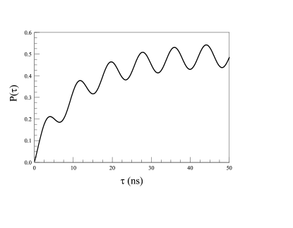
Figure 3: The probability (III.25) for $t_{d}=7\,\mathrm{ns}~{},~{}\Delta\omega=2\pi\times 122\,\mathrm{MHz}~{};~{}1/\Gamma=12\,\mathrm{ns}$.

This figure reveals the effect of which-path suppression of the coherence: the asymptotic behavior of the probability is

$$\frac{{P}_{M|H}(\tau\gg 1/\Gamma)}{\mathcal{D}(\Omega)}\simeq\frac{1}{2}\Big{[}1+\frac{\Gamma}{\Delta\omega}\,\sin\big{[}\Delta\omega(\tau+t_{d})\big{]}\Big{]}\,.$$ (III.26)

Measurement in the $H/V$ basis results in a post-measurement density matrix that features coherence in the qubit basis $|\pm 1\rangle$ suppressed by which-path information. This coherence was not manifest in the pre-measurement density matrix because of the orthogonality of the circularly polarized photon wave packets.

The reduced density matrix (III.20) is similar to (II.26), normalizing so that $\widetilde{\rho}_{D}(\tau)=\rho_{D}(\tau)/\mathrm{Tr}\rho_{D}(\tau)$ it can be diagonalized in a new basis that differs from (II.47,II.48) by the phases multiplying $|-1\rangle$ and with eigenvalues

$$\epsilon_{\pm}(\tau)=\frac{1}{2}\Big{[}1\pm|\eta(\tau)|\Big{]}$$ (III.27)

respectively, leading to the post-photodetection Von-Neumann entropy of entanglement

$$\widetilde{S}_{D}(\tau)=-\mathrm{Tr}\widetilde{\rho}_{D}(\tau)\ln\widetilde{\rho}_{D}(\tau)=-\epsilon_{+}(\tau)\ln\epsilon_{+}(\tau)-\epsilon_{-}(\tau)\ln\epsilon_{-}(\tau)\,.$$ (III.28)

This post-measurement entanglement entropy is given by $S_{fo}(\infty)$ in eqn. (II.51) asymptotically for $\Gamma\tau\gg 1$ .

III.1 Implementing a “Quantum eraser”:

The factor $1/(1+i\Delta\omega/\Gamma)$ in the results (III.20,III.22,II.27) reflects which-path information because it suppresses coherence when $\Delta\omega\gg\Gamma$. It is noteworthy that this suppression remains in the final expressions even in an “ideal” broadband photodetector a lá Glauber which is insensitive to the photon frequency and with a photodetection correlation function $\propto\delta(t-t^{\prime})$ as discussed above.

In the experiment in ref.dutt $\Delta\omega=2\pi\times 122\,\mathrm{MHz}~{}~{};~{}~{}\Gamma\simeq 1/12\,\mathrm{ns}$ so that $\Delta\omega/\Gamma\simeq 9.2$ and there is a strong suppression of coherence because of which-path information $1/\sqrt{1+\Delta\omega^{2}/\Gamma^{2}}\simeq 0.11$. In this experiment photodetection is carried out with a photodetector with time resolution $\delta t\simeq 300\,\mathrm{ps}\ll 1/\Delta\omega$ to implement a “quantum eraser”eraser1 ; eraser2 to “erase” which-path information by introducing an energy uncertainty $\sim 1/\delta t\gg\Delta\omega$.

A simple model for such photodetector can be implemented by modifying the interaction Hamiltonian between the detector and the radiation field $H_{DR}$ (III.1) introducing a “shutter function” $\mathds{S}(t)$ with explicit time dependence, namely

$$H_{DR}(t)=\sum_{j}\Big{[}\vec{d}_{j}\cdot\vec{E}^{(+)}_{P}(\vec{x}_{d};t)|e^{d}_{j}\rangle\langle g^{d}|\,e^{i\nu_{j}t}+\mathrm{h.c.}\Big{]}\,\mathds{S}(t)~{}~{};~{}~{}P=H;V\,,$$ (III.29)

where the only restrictions on the shutter function $\mathds{S}(t)$ are

$$\mathds{S}(t)=\Bigg{\{}\begin{array}[]{l}\sim 1~{}~{}t_{D}-\delta t\leq t\leq t_{D}\\ 0~{}~{}\mathrm{otherwise}\end{array}$$ (III.30)

with the shutter interval $\delta t$ such that

$$\Gamma\delta t\ll\Delta\omega\delta t\ll 1\,.$$ (III.31)

This function effectively describes a shutter with a time resolution $\delta t$ and amounts to “slicing” or time-binning the photon wavefunction upon detection.

A similar procedure of “chopping” the wave function in short time intervals has also been advocated as a quantum eraser in ref.sham1 . In ref.mismatch a phenomenological damping term is added to the right hand side of the equivalent of equations (A.4) in this reference, with the argument that such damping term describes the coupling of the (single) excited state of the detector atom to some reservoir. A “quantum eraser” is implemented in this approach by taking the damping constant $\gamma\gg\Delta\omega$. While this phenomenological approach seems sensible, we consider instead the model of the photodetector with the shutter function $\mathds{S}(t)$ introduced above implemented within an ideal broadband photodetector as follows.

The solution for the coefficients $D_{j,\pm}(t_{D})$ are now given by

$$D_{j,\pm}(t_{D})=-i\frac{\vec{d}_{j}}{\sqrt{2}}\cdot\int_{0}^{t_{D}}\langle 0_{\gamma}|\vec{E}^{(+)}_{P}(\vec{x}_{d},t)|\sigma_{\mp}(t)\rangle\,\mathds{S}(t)\,\,e^{i\nu_{j}t}dt\,,$$ (III.32)

and the reduced density matrix elements in (III.14) become

$$\sum_{j}D_{j,a}(t_{D})D^{*}_{j,b}(t_{D}) = \frac{1}{2}\int_{0}^{t_{D}}dt\int_{0}^{t_{D}}dt^{\prime}~{}\mathds{S}(t)\,\mathds{S}(t^{\prime})\langle\sigma_{b}(t)|E^{(-)}(\vec{x_{d}},t)E^{(+)}(\vec{x_{d}},t^{\prime})|\sigma_{a}(t^{\prime})\rangle$$ (III.33)

$$\times \int_{-\infty}^{\infty}\mathcal{D}(\omega)e^{i\omega(t-t^{\prime})}\,d\omega~{}~{};~{}~{}a,b=+,-\,,$$

where we have used that $|\sigma_{\pm}(t)\rangle$ are one-photon wavepackets and only the vacuum contributes to the intermediate state in the correlation function of the electric field. The last term in (III.33) is the photodetector correlation function book1 ; book2 which for a broadband photodetector is given by eqn. (III.18), leading to

$$\sum_{j}D_{j,a}(t_{D})D^{*}_{j,b}(t_{D}) = 2\pi\,\frac{\mathcal{D}(\Omega)}{2}\int_{0}^{t_{D}}dt\mathds{S}^{2}(t)\,\langle\sigma_{b}(t)|E^{(-)}_{P}(\vec{x_{d}},t)E^{(+)}_{P}(\vec{x_{d}},t)|\sigma_{a}(t)\rangle$$ (III.34)

$$\simeq 2\pi\,\frac{\mathcal{D}(\Omega)}{2}\langle\sigma_{b}(t_{D})|E^{(-)}_{P}(\vec{x_{d}},t_{D})E^{(+)}_{P}(\vec{x_{d}},t_{D})|\sigma_{a}(t_{D})\rangle\,\delta t\,.$$

where we have used the condition (III.31) so that the integrand is constant in the interval $t_{D}-\delta t\leq t\leq t_{D}$ and vanishes outside it. Using the result (A.5) we obtain the reduced density matrix in the Schroedinger picture

$$\rho_{D}(t_{D})=\frac{\mathcal{D}(\Omega)}{2}\,\Big{(}\Gamma\delta t\Big{)}\,\,e^{-\Gamma\tau}~{}\Theta(\tau)~{}\Bigg{\{}|+1\rangle\langle+1|+|-1\rangle\langle-1|+\delta^{P}_{-}~{}\Big{(}|+1\rangle\langle-1|\,e^{i\Delta\omega\,t_{d}}+\mathrm{h.c.}\Big{)}\Bigg{\}}\,.$$ (III.35)

Remarkably, this density matrix describes a pure state, namely

$$\rho_{D}(t_{D})=\mathcal{N}(\tau)~{}\Big{(}e^{i\Omega_{+}t_{d}}|+1\rangle+\delta^{P}_{-}\,e^{i\Omega_{-}t_{d}}|-1\rangle\Big{)}\Big{(}e^{-i\Omega_{+}t_{d}}\langle+1|+\delta^{P}_{-}\,e^{-i\Omega_{-}t_{d}}\langle-1|\Big{)}$$ (III.36)

with the normalization

$$\mathcal{N}(\tau)=\frac{\mathcal{D}(\Omega)}{2}\,\Big{(}\Gamma\delta t\Big{)}\,\,e^{-\Gamma\tau}~{}\Theta(\tau)~{}~{};~{}~{}\tau=t_{D}-t_{d}\,.$$ (III.37)

It is noteworthy that the quantum eraser has purified the post-measurement reduced density matrix. This analysis confirms the experimental results in refs.dutt ; qdotyama and bolsters the arguments presented in ref.qdotyama .

In the experiment in ref.dutt after detection the spin-qubit evolves freely in time from $t_{D}$ until a time $t$ so that

$$\rho_{D}(t)=\mathcal{N}(\tau)~{}\Big{(}e^{i\Omega_{+}(t-\tau)}|+1\rangle+\delta^{P}_{-}\,e^{i\Omega_{-}(t-\tau)}|-1\rangle\Big{)}\Big{(}e^{-i\Omega_{+}(t-\tau)}\langle+1|+\delta^{P}_{-}\,e^{-i\Omega_{-}(t-\tau)}\langle-1|\Big{)}$$ (III.38)

at which time two microwave pulses resonant with the levels $|\pm\rangle$ are turned on and transfer coherently the state

$$|M(t)\rangle=\frac{1}{\sqrt{2}}\Big{(}e^{i\Omega_{+}t}|+1\rangle+e^{i\Omega_{-}t}e^{i\phi}|-1\rangle\Big{)}$$ (III.39)

with a fixed phase $\phi$ to the ground state $|0\rangle$, as depicted in fig. (4).

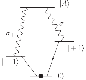
Figure 4: Coherent transfer of the state $|M(t)\rangle$ to the ground state $|0\rangle$ see ref.dutt .

Now we find the total (joint) probability

$$P_{M|H,V}(\tau)=Tr\Big{[}\rho_{D}(t)|M(t)\rangle\langle M(t)|\Big{]}=\frac{\mathcal{N}(\tau)}{2}~{}\Big{[}1\pm\cos\alpha(\tau)\Big{]}~{}~{};~{}~{}\alpha(\tau)=\Delta\omega~{}\tau+\phi\,.$$ (III.40)

This result agrees with the joint probability quoted and experimentally confirmed in ref.dutt up to the overall normalization factor and the retardation in the detection time $\tau=t_{D}-t_{d}$.

IV Summary and conclusions:

In this article we have studied the dynamics of frequency and polarization entanglement between photons and a spin-qubit from spontaneous decay in a typical $\Lambda$ system with non-degenerate lower levels. We addressed in detail how which path information affects coherence, obtained the entanglement entropy for the reduced spin-qubit with frequency and polarization entanglement and provided a unified description of the process of spontaneous emission and broadband photodetection that is fully causal and allows to include a quantum eraser in a consistent manner.

The main results are the following: beginning with the case in which photon spin-qubit entanglement does not involve polarization but only frequency, the reduced qubit density matrix obtained from tracing out the radiation bath features oscillatory coherence terms (in the qubit basis) that are suppressed by which path information by a factor $1/\sqrt{1+\Delta\omega^{2}/\Gamma^{2}}$ where $\Delta\omega$ is the Zeeman splitting between the lower spin states and $\Gamma$ is the linewidth of the excited state. In the case in which the spin degree of freedom is entangled with circularly polarized photons, the reduced density matrix is a statistical mixture as a consequence of the orthogonality of the polarization of the photon states. We obtain the entanglement Von-Neumann entropy in both cases and analyze their long time asymptotic behavior. In the case in which the spontaneous decay rate is the same to the two lower levels, we find that $S_{fp}(t)\geq S_{fo}(t)$ where $S_{fp}(t)$ ($S_{fo}(t)$) is the entanglement entropy for frequency and polarization (frequency only). Focusing on broadband photodetection in the case of frequency and polarization entanglement, we find that with an ideal photodetector that filters photons with horizontal (H) or vertical (V) directions the post-measurement density matrix describes a mixed state with non-vanishing coherences in the qubit basis. Despite the broadband nature of the photodetector described by correlation function $\propto\delta(t-t^{\prime})$, the coherences display oscillatory behavior suppressed by which path information just as the pre-measurement density matrix in the case of frequency entanglement.

A “quantum eraser” is implemented within the Glauber model of broadband photodetection by including a “shutter function” that effectively time-bins photodetection with a time resolution $\delta t$ so that $\Gamma\delta t\ll\Delta\omega\delta t\ll 1$ thereby introducing enough energy uncertainty to average out frequency information. We find that photodetection with this “quantum eraser” purifies the post-measurement reduced density matrix to a pure state. The resulting joint probability for $H/V$ photodetection with projection onto a a superposition of qubit states $|M(t)\rangle=\frac{1}{\sqrt{2}}\Big{(}e^{i\Omega_{+}t}|+1\rangle+e^{i\Omega_{-}t}e^{i\phi}|-1\rangle\Big{)}$ is given by (III.40) and agrees with the experimental results found in ref.dutt .

Several aspects of the results obtained in this article suggest possible experimental avenues: 1) the dependence on the delay time $t_{d}=x_{d}/c$ with $x_{d}$ the position of the photodetector, suggests the possibility of using several photodetectors in coincidence, for example to study interference effects, Hanbury-Brown-Twiss correlations or as a complementary variable to explore coherence as a function of this delay distance, 2) rather than implementing a “quantum eraser” with time-binned photodetection, continuous photodetection should instead produce a joint probability given by (III.25) which displays steps in the coherent oscillations (see fig. (3)), 3) instead of a “quantum eraser” with time resolution $\delta t\ll 1/\Delta\omega$ one could consider a “quantum blurrer” with a varying shutter time resolution. This serves as a window to let more which path information thereby suppressing the coherence in a controlled manner.

The experimental relevance of the questions studied in this article merit further study perhaps including alternative methods such as those of quantum open systems in terms of a master equationzoeller ; dalibard or “quantum jumps” followed by density matrix resetting as advocated in ref.heger .

Entanglement and quantum correlations are becoming very important in many timely aspects of particle physics: in neutrino oscillationsnu1 ; nu2 and in CP and T violationtviolent ; Bo . Recently the entanglement of neutral B-meson pairs produced from the (spontaneous) decay of a $\Upsilon(4S)$ resonance has been exploited experimentally to unambiguously show time-reversal violationtrevbo ; babar by tagging individual members of the correlated pairs. Therefore the interest on the dynamics of entanglement, the emergence of spontaneous coherence and quantum correlations is transcending disciplines and clearly merits deeper understanding.

Appendix A Solutions for the coefficients in eqn. (III.11,III.12)

The equations of motion for the coefficients in eqn. (III.11,III.12) are obtained from the Schroedinger equation in the interaction picture $d|\Psi(t)\rangle/dt=-iH_{I}(t)|\Psi(t)\rangle$ projecting on the corresponding states.

These simplify substantially from the following properties: $H_{AR}$ is the identity in the detector space $\{|e^{d}_{j}\rangle,|g^{d}\rangle\}$ and $H_{DR}$ is the identity in the NV-center basis $\{|A\rangle,|\pm 1\rangle\}$.

The equations of motion for the coefficients $C_{\vec{k},\pm}(t)$ feature contributions of the form

$$\langle 1_{\vec{k},\pm};\mp 1;g^{d}|H_{DR}|\mp 1;e^{d}_{j};0_{\gamma}\rangle\,D_{j,\mp}(t)$$

arising from the term $\sum_{j}\vec{d}^{*}_{j}\cdot\vec{E}^{(-)}(\vec{x}_{d},t)|g^{d}\rangle\langle e^{d}_{j}|$ in $H_{DR}(t)$. Such term describes the de-excitation of the photodetector by spontaneous emission from an excited state $|e^{d}_{j}\rangle$ in which the NV-center states $|\pm 1\rangle$ are passive, this term is of higher order in dipolar couplings and under the assumption of very small detection efficiency as is the case experimentally (see below) it will be neglected, leading to the final form of the equations of motion

$$i\dot{C}_{A}(t) = \langle A;0_{\gamma}|H_{AR}(t)|1_{\vec{k},+};-1\rangle\,{C}_{\vec{k},-}(t)+\langle A;0_{\gamma}|H_{AR}(t)|1_{\vec{k},-};+1\rangle\,{C}_{\vec{k},+}(t)$$ (A.1)

$$i\dot{C}_{\vec{k},+}(t) = \langle 1_{\vec{k},-};+1|H_{AR}(t)|A;0_{\gamma}\rangle\,{C}_{A}(t)$$ (A.2)

$$i\dot{C}_{\vec{k},-}(t) = \langle 1_{\vec{k},+};-1|H_{AR}(t)|A;0_{\gamma}\rangle\,{C}_{A}(t)$$ (A.3)

$$\dot{D}_{j,\pm}(t) = -i\frac{\vec{d}_{j}}{\sqrt{2}}\cdot\langle 0_{\gamma}|\vec{E}^{(+)}_{P}(\vec{x}_{d},t)|\sigma_{\mp}(t)\rangle\,\,e^{i\nu_{j}t}\,,$$ (A.4)

where the states $|\sigma_{\mp}(t)\rangle$ are given by (II.41) with (II.36) evaluated at $\vec{x}_{0}=\vec{0}$. The solutions to eqns. (A.1,A.2,A.3) are the same as (II.35,II.36). Upon inserting these solutions in the matrix element (A.4), we obtain in the Wigner-Weisskopf approximation

$$-i\frac{\vec{d}_{j}}{\sqrt{2}}\cdot\langle 0_{\gamma}|\vec{E}^{(+)}_{P}(\vec{x}_{d},t)|\sigma_{\mp}(t)\rangle\,\,e^{i\nu_{j}t}=\kappa_{j}~{}\sqrt{\frac{\Gamma_{\pm}}{2\pi}}~{}\delta^{P}_{\mp}\,e^{i\nu_{j}t_{d}}~{}e^{i(\nu_{j}-\Omega_{\pm})(t-t_{d})}\,e^{-\frac{\Gamma}{2}(t-t_{d})}\,\Theta(t-t_{d})~{}~{};~{}~{}t_{d}=\frac{x_{d}}{c}$$ (A.5)

where the constants $\kappa_{j}$ are proportional to $d_{j}/x_{d}$ with proportionality coefficients that result from angular and contour integration and

$$\delta^{P}_{\mp}=\Bigg{\{}\begin{array}[]{c}1~{}~{}\mathrm{for}~{}~{}P=H\\ \mp\,1~{}~{}\mathrm{for}~{}~{}P=V\end{array}\,.$$ (A.6)

From this result we obtain

$$D_{j,\pm}(t)=i\kappa_{j}~{}\sqrt{\frac{\Gamma_{\pm}}{2\pi}}~{}\delta^{P}_{\mp}\,e^{i\nu_{j}t_{d}}~{}\frac{\Big{[}1-e^{i(\nu_{j}-\Omega_{\pm}+i\frac{\Gamma}{2})(t-t_{d})}\Big{]}}{\Big{[}\nu_{j}-\Omega_{\pm}+i\,\frac{\Gamma}{2}\Big{]}}~{}\Theta(t-t_{d})\,.$$ (A.7)

References

• (1) A. Einstein, B. Podolsky, N. Rosen, Phys. Rev. 47, 777 (1935).
• (2) Nielsen M A and Chuang I L, Quantum Computation and Quantum Information (Cambridge: Cambridge University Press, 2000).
• (3) H. J. Kimble, Nature 453, 1023 (2008).
• (4) L. M. Duan, C. Monroe, Rev. Mod. Phys. 82, 1209 (2010).
• (5) S. J. Van Enk, N. Lutkenhaus, H. J. Kimble, Phys. Rev. A 75, 052318 (2007).
• (6) R. Horodecki, P. Horodecki, M. Horodecki, K. Horodecki, Rev.Mod.Phys.81, 865 (2009).
• (7) M. C. Tichy, F. Mintert, A. Buchleitner, J. Phys. B: At. Mol. Opt. Phys. 44 192001 (2011).
• (8) B. B. Blinov, D. L. Moehring, L. M. Duan, C. Monroe, Nature, 428, 153 (2004).
• (9) J. Volz et.al. Phys. Rev. Lett. 96, 030404 (2006).
• (10) T. Wilk, S. C. Webster, A. Kuhn, G. Rempe, Science 317, 488 (2007).
• (11) D. Matsukevich, et.al. Phys. Rev. Lett. 95, 040405 (2005).
• (12) D. L. Moehring et.al. Nature 449, 68 (2007).
• (13) L.-M. Duan, M. D. Lukin, J. I. Cirac, P. Zoller, Nature 414, 413(2001).
• (14) C. Cabrillo, J.I. Cirac,P. Garcia-Fernandez, P. Zoeller, Phys. Rev. A59, 1025 (1999).
• (15) A. Stute, et.al. arXiv:1301.0490
• (16) A. Stute, et.al. Nature 485, 482 (2012).
• (17) H. Walther, B. T. H. Varcoe, B.-G. Englert, T. Becker, Rep. Prog. Phys. 69 1325, (2006).
• (18) C. Flindt, A. S. Sorensen, M. D. Lukin, J. M. Taylor, Phys. Rev. Lett. 98, 240501 (2007).
• (19) E. Togan et.al., Nature 466, 730, (2010).
• (20) K. De Greve, et.al. Nature 491, 421 (2012).
• (21) W. B. Gao, et.al. Nature 491,426 (2012).
• (22) J. R. Schaibley et.al. arXiv:1210.5555.
• (23) J. Javanainen, Europhys. Lett. 17, 407 (1992).
• (24) S. E. Economou, R-B. Liu, L. J. Sham, D. G. Steel, Phys. Rev. B71, 195327 (2005).
• (25) W. Yao, R. -B. Liu, L. J. Sham, Phys. Rev. Lett. 95, 030504 (2005).
• (26) M. V. G. Dutt et.al. Phys. Rev. Lett.94, 227403 (2005).
• (27) A. Imamoglu et.al. Phys. Rev. Lett. 83, 4204 (1999).
• (28) A. Chabaev, Al. L. Efros, D. Gammon, I. A. Merkulov, Phys. Rev. B68, 201305(R) (2003).
• (29) P. Chen, C. Piermarocchi, L. J. Sham, D. Gammon, D. G. Steel, Phys. Rev. B69, 075320 (2004).
• (30) J. R. Schaibley, P. R. Berman, J. Phys. B: At. Mol. Opt. Phys. 45, 124020 (2012).
• (31) P. W. Milonni, D. F. V. James, H. Fearn, Phys. Rev. A 52, 1525 (1995).
• (32) M. O. Scully, K. Druhl, Phys. Rev. A 25, 2208 (1982).
• (33) Y.-H. Kim, R. Yu, S.P. Kulik, Y.H. Shih, M. O. Scully, Phys.Rev.Lett.84, 1 (2000).
• (34) M. O. Scully, M. S.Zubairy, Quantum Optics, (Cambridge University Press, UK, 1997).
• (35) C.Cohen-Tannoudji, J. Dupont-Roc,G. Grynberg, Atom-Photon Interactions, Basic Processes and Applications (John Wiley, N.Y. 1998).
• (36) R. J. Glauber, Phys. Rev. 130, 2529 (1963); Phys. Rev. 131, 2766 (1963); Quantum Optics and Electronics (Ed. C. DeWitt, A. Blandin, C. Cohen-Tannoudji; Gordon and Breach, N.Y. 1965).
• (37) V. Weisskopf and E. Wigner, Z. Phys. 63, 54, (1930).
• (38) C. W.Gardiner, P. Zoller Quantum Noise(Springer, Berlin, 2004).
• (39) J. Dalibard, Y. Castin, K. Molner, Phys. Rev. Lett.68, 580 (1992).
• (40) G. C. Hegerfeldt, Phys. Rev. A. 47, 449 (1993).
• (41) A. G. Cohen, . L. Glashow, Z. Ligeti, Phys.Lett.B678, 191 (2009).
• (42) D. Boyanovsky, Physical Review D 84, 065001 (2011); L. Lello, D. Boyanovsky, arXiv:1208.5559; J. Wu, J. A. Hutasoit, D. Boyanovsky, R. Holman, Phys. Rev.D82, 013006 (2010), Int. J. Mod. Phys. A 26, 5261 (2011).
• (43) J. Bernabeu, F. Martinez-Vidal, P. Villanueva-Perez, JHEP 1208, 064 (2012).
• (44) A. Go (for the Belle collaboration), Phys.Rev.Lett. 99, 131802 (2007).
• (45) J. P. Lees (BaBar Collaboration), arXiv:1207.5832.
• (46) Ray F. Cowan, for the BABAR Collaboration, arXiv:1301.1372