A semiparametric regression model for paired longitudinal outcomes with application in childhood blood pressure development

Abstract

This research examines the simultaneous influences of height and weight on longitudinally measured systolic and diastolic blood pressure in children. Previous studies have shown that both height and weight are positively associated with blood pressure. In children, however, the concurrent increases of height and weight have made it all but impossible to discern the effect of height from that of weight. To better understand these influences, we propose to examine the joint effect of height and weight on blood pressure. Bivariate thin plate spline surfaces are used to accommodate the potentially nonlinear effects as well as the interaction between height and weight. Moreover, we consider a joint model for paired blood pressure measures, that is, systolic and diastolic blood pressure, to account for the underlying correlation between the two measures within the same individual. The bivariate spline surfaces are allowed to vary across different groups of interest. We have developed related model fitting and inference procedures. The proposed method is used to analyze data from a real clinical investigation.

T1Supported by Grant R01 HL095086 from the National Heart, Lung, and Blood Institute, United States Department of Health and Human Services.

and

1 Introduction

Excess weight gain has long been recognized as a risk factor for metabolic and cardiovascular disorders, including hypertension. Population studies have shown that weight strongly predicts blood pressure [Huang et al. (1998), Masuo et al. (2000)], although the relationship between the two may not be linear [Hall et al. (2010)]. Data from children and young adults are equally persuasive on the weight–blood pressure association [Stray-Pedersen et al. (2009), Levin et al. (2010)]. In fact, the observations are so consistent that some even question whether obesity and hypertension are two epidemics or one [Davy and Hall (2004)]. More recently, an increasing number of studies have recognized a similarly salient relationship between height and blood pressure [Shankar et al. (2005), Fujita et al. (2010)]. Although this latter relationship appears to have a seemingly plausible physiological interpretation (taller individuals need greater pressure to maintain oxygenated blood flow to the head and upper extremities), the concurrent increases of height and weight have nonetheless made it analytically difficult to discern the effect of weight from that of height. The matter is further complicated by the observed significantly positive effect of body mass index (BMI, defined as Weight$/$Height²) on blood pressure, as shown in numerous studies [Lauer and Clarke (1989), Baker, Olsen and Sorensen (2007), Falkner (2010)]. In fact, overweight and obesity, clinically defined by BMI cutoff points, have been recognized as major risk factors for hypertension, and, indeed, hypertension prevalence is much higher in overweight and obese children [Falkner et al. (2006), Steinberger et al. (2009)]. Therefore, the scientific community has a great interest to elucidate the independent influences of height and weight on blood pressure, as they may implicate different pathophysiology for this etiologically less understood disease. For example, an obesity mediated blood pressure elevation would implicate a more activated sympathetic nervous system (perhaps stimulated by adipose-derived hormones such as leptin), and increased sodium reabsorption by the kidney [Hall et al. (2010)], whereas a strong height influence could give more credence to the notion that the disease has its origin in growth [Lever and Harrap (1992)].

In this research, we assess the simultaneous influences of height and weight on blood pressure using prospectively collected data from a cohort of healthy children. Such an exercise, however, faces a number of methodological challenges: (1) Outcomes are repeatedly measured paired observations. Blood pressure consists of two readings, a systolic measurement taken during the contraction phase of the cardiac cycle and a diastolic measurement taken during the recoil phase of the cardiac cycle. Together, they represent the pressure exerted by the circulating blood on the walls of blood vessels during two different phases of the same cardiac cycle. For longitudinally collected blood pressure measurements, separate modeling of the systolic and diastolic outcomes may not be appropriate, as the two are biologically correlated and mutually influential [Guo and Carlin (2004)]. (2) Height and weight effects on blood pressure may be nonlinear. Previous research has recognized a nonlinear pattern of the adiposity effects on blood pressure [Hall (2003)]. More recent data indicate a nonlinear height effect on blood pressure as well [Tu et al. (2009)]. Preliminary data from this investigation also indicate nonlinear height and weight effects on blood pressure; see Figure 1 in Section 5. Furthermore, interaction of height and weight may exist. To accommodate, nonlinear bivariate effect surfaces will have to be incorporated into the model for the purpose of depicting the joint height–weight effects on blood pressure. (3) Inferences are needed for comparing the joint height–weight effects across different gender and ethnicity groups. Such comparisons are of great interest, as recent reports indicate significantly higher risks of obesity and hypertension in black children than in white children [Anderson and Whitaker (2009), Brady et al. (2010)]. Differentially expressed bivariate effect surfaces, therefore, may well point to different pathophysiology of the disease among people of different ethnic backgrounds.

To address these challenges, we propose a joint semiparametric mixed effects model that includes two individual components, one for systolic and the other for diastolic blood pressure measures. Bivariate smooth functions for the joint height–weight effects are embedded in these components to account for possible nonlinear effects as well as interactions between the two independent variables. The two components are then connected by shared random subject effects in a unified regression framework.

Semiparametric regression as a practical data analytical tool has experienced tremendous growth in the past ten years, especially since the publication of the book Semiparametric Regression by Ruppert, Wand and Carroll (2003). Methodological extensions, stimulated by exciting applications, and new computational approaches, have now covered most commonly encountered data situations. He, Fung and Zhu (2005) considered robust generalized estimating equations (GEE) for analyzing longitudinal data in generalized partial linear models. Lin and Carroll (2006) proposed profile kernel and backfitting estimation methods for a class of semiparametric problems. Models with bivariate smoothing have been developed for geospatial [Sain et al. (2006), Guillas and Lai (2010)] and medical imaging applications [Brezger, Fahrmeir and Hennerfeind (2007)]. Penalized splines have been used to analyze longitudinally measured event counts [Dean, Nathoo and Nielsen (2007)]. Crainiceanu, Diggle and Rowlingson (2008) have proposed penalized bivariate splines for binary response and developed related Bayesian inference procedures. More recently, Ghosh and Tu (2009) have developed a joint semiparametric structure for zero-inflated counts that consists of a logistic model for the proportion of zeros and a log-linear model for Poisson counts; both models contain univariate nonparametric components. Ghosh and Hanson (2010) studied a semiparametric model for multivariate longitudinal data in a Bayesian framework. Although there is a rich literature on semiparametric analysis of longitudinal (or clustered) data, not much has been developed for analyzing bivariate joint effects of two continuous independent variables (height and weight in this application) on a pair of closely related outcome variables (e.g., systolic and diastolic blood pressure). The current research extends the previous work by introducing group-specific bivariate smooth components into the joint modeling of paired outcomes. Related model fitting and inference procedures are also developed.

The outline of this paper is as follows. We introduce the semiparametric mixed model for paired outcomes and its estimation in Section 2. Hypothesis testing for group differences in the bivariate effect surfaces is discussed in Section 3, followed by a Monte Carlo study in Section 4. As the motivation and illustration of the proposed methods, a real data application of childhood blood pressure study is presented in Section 5. We conclude the paper with a few methodological and scientific remarks in Section 6. Additional details on model-fitting algorithms and model diagnostics are provided in the supplementary materials [Liu and Tu (2012)].

2 Methods

2.1 A semiparametric mixed model for paired outcomes

We introduce our model in a more generic setting. Let $\mathbf{Y}_{ij}=(Y^{(1)}_{ij},Y^{(2)}_{ij})^{T}$ be a pair of outcomes from the $i$th subject measured at the $j$th visit, where $j=1,\ldots,n_{i}$ and $i=1,\ldots,m$. Assuming that we have $g=1,\dots,G$ groups of interest, let $z_{ig}$ be a binary group indicator for the $i$th subject: $z_{ig}=1$ if the $i$th subject belongs to the $g$th group, $z_{ig}=0$ otherwise. We propose the following semiparametric mixed effects model for the paired outcomes:

$$\cases{\displaystyle Y^{(1)}_{ij}=U^{(1)}_{i}+\mathbf{t}_{ij}^{T}\bolds{\psi}_{1}+\sum_{g=1}^{G}f^{(1)}_{g}(w_{ij},h_{ij})z_{ig}+\epsilon^{(1)}_{ij},\vspace*{2pt}\cr\displaystyle Y^{(2)}_{ij}=U^{(2)}_{i}+\mathbf{t}_{ij}^{T}\bolds{\psi}_{2}+\sum_{g=1}^{G}f^{(2)}_{g}(w_{ij},h_{ij})z_{ig}+\epsilon^{(2)}_{ij},}$$ (1)

where $\widetilde{\mathbf{U}}_{i}=(U^{(1)}_{i},U^{(2)}_{i})^{T}$ is the random subject effect vector; $\mathbf{t}_{ij}$ denotes the time-varying covariate vector of the $i$th subject at visit $j$ whose effects are assumed to be parametric with corresponding parameter vectors $\bolds{\psi}_{1}$ and $\bolds{\psi}_{2}$; the joint influences of two continuous independent variables $w_{ij}$ and $h_{ij}$ in each group are modeled by the group-specific bivariate smooth functions $f^{(1)}_{g}$ and $f^{(2)}_{g}$ for the paired outcomes respectively; $\epsilon^{(1)}_{ij}$ and $\epsilon^{(2)}_{ij}$ are random errors. Herein, we let $\mu^{(1)}_{ij}=\mathbf{t}_{ij}^{T}\bolds{\psi}_{1}+\sum_{g=1}^{G}f^{(1)}_{g}(w_{ij},h_{ij})z_{ig}$ and $\mu^{(2)}_{ij}=\mathbf{t}_{ij}^{T}\bolds{\psi}_{2}+\sum_{g=1}^{G}f^{(2)}_{g}(w_{ij},h_{ij})z_{ig}$ to denote the mean responses.

The regression equations of the paired outcomes in (1) are connected via the shared random effect vector $\widetilde{\mathbf{U}}_{i}$, which is used to account for not only the correlation among the repeated measurements from the same subject, but also the correlation between the two outcome variables. The subject-specific random effect is assumed to be independently normally distributed, that is, $\widetilde{\mathbf{U}}_{i}\sim\mathcal{N}(\mathbf{0},\bolds{\Sigma}_{u})$, with variance–covariance matrix

$$\bolds{\Sigma}_{u}=\pmatrix{\sigma_{1}^{2}&\rho\sigma_{1}\sigma_{2}\vspace*{2pt}\cr\rho\sigma_{1}\sigma_{2}&\sigma_{2}^{2}},$$ (2)

where $\sigma_{1}^{2}$ and $\sigma_{2}^{2}$ are two variance components, and $\rho$ is the correlation coefficient of the random subject effects of the paired outcomes $Y^{(1)}_{ij}$ and $Y^{(2)}_{ij}$ from the same subject measured at one visit. The correlation structure allows us to jointly examine the two closely related clinical outcomes in a unified modeling framework. The within-subject random errors associated with $Y^{(1)}_{ij}$ and $Y^{(2)}_{ij}$, namely, $\epsilon_{ij}^{(1)}$ and $\epsilon_{ij}^{(2)}$, are assumed to follow two independent stochastic processes that could possibly lead to serial correlation within each error series. In general, a wide range of correlation structures could be embedded into the errors by assuming, for example, $\operatorname{cor}(\epsilon_{ij}^{(l)},\epsilon_{ij^{\prime}}^{(l)})=q(d(\mathbf{s}_{ij},\mathbf{s}_{ij^{\prime}}),\bolds{\phi})$, $l=1,2,$ where $q$ is a correlation function taking values between $-1$ and $1$, $d$ is some distance measure of the two position vectors $\mathbf{s}_{ij}$ and $\mathbf{s}_{ij^{\prime}}$ associated with $\epsilon_{ij}^{(l)}$ and $\epsilon_{ij^{\prime}}^{(l)}$, respectively, and $\bolds{\phi}$ denotes a vector of correlation parameters. Without loss of generality, in the following discussion on model estimation we assume simple independent errors with normal distribution $(\epsilon_{ij}^{(1)},\epsilon_{ij}^{(2)})^{T}\sim\mathcal{N}(\mathbf{0},\bolds{\Sigma}_{\epsilon})$, where $\bolds{\Sigma}_{\epsilon}=\sigma_{\epsilon}^{2}\operatorname{diag}(1,\delta^{2})$ with the dispersion parameter $\sigma_{\epsilon}^{2}$ and a relative scale parameter $\delta$ for modeling heteroscedasticity of the random errors associated with the two outcomes. More general error processes including autoregressive moving-average ($\operatorname{ARMA}$) and continuous time autoregressive structures can be introduced into the current modeling framework, which will be revisited at the end of Section 2.3.

In (1) we assume a compound symmetry covariance for the random subject effects, which implies that the correlation between the two random effects corresponding to the paired outcomes remains constant over time. If necessary, serial correlations among repeated measures from the same individual could be specified by the within-subject error structure. In this study, we are primary interested in the effect of somatic growth on blood pressure development in children, both of which increase with age. Hence, we opt not to explicitly introduce temporal effects into the model. In applications where time trajectories are of primary interest, time-varying correlation structures can be incorporated if constant correlation assumption is not adequate. See Morris et al. (2001) and Dubin and Müller (2005) for related discussion on the modeling of varying correlations between random functions.

2.2 Nonparametric smooth functions

In the proposed semiparametric mixed model (1), the group-specific bivariate smooth functions are represented by linear combinations of some generic basis functions as follows:

$$f^{(1)}_{g}(w,h)=\sum_{k=0}^{K}b_{k}(w,h)\beta_{gk},\qquad f^{(2)}_{g}(w,h)=\sum_{k=0}^{K}c_{k}(w,h)\gamma_{gk},$$

where $b_{0}=c_{0}=1$, $b_{k}(w,h)$ and $c_{k}(w,h),k=1,\ldots,K$, are the basis functions of any bivariate smoother; $\bolds{\beta}_{g}=(\beta_{g0},\ldots,\beta_{gK})^{T}$, $\bolds{\gamma}_{g}=(\gamma_{g0},\ldots,\gamma_{gK})^{T},g=1,\ldots,G,$ are regression coefficients associated with the nonparametric components in each group. Note that $(\beta_{10},\ldots,\beta_{G0})$ and $(\gamma_{10},\ldots,\gamma_{G0})$ represent, respectively, the population average of the paired outcomes in different groups. In this research, we choose to use a thin plate spline as the bivariate smoother [Wood (2003)], which is computationally more convenient for modeling high-dimensional nonparametric functions. The thin plate regression splines in a semiparametric model can be estimated via the penalized likelihood approach [Green and Silverman (1994)]. The penalized log-likelihood function of model (1) can be written as

$$\ell_{p}=\ell-\sum_{g=1}^{G}\lambda_{g}J\bigl{(}f^{(1)}_{g}\bigr{)}-\sum_{g=1}^{G}\varphi_{g}J\bigl{(}f^{(2)}_{g}\bigr{)},\vspace*{-1pt}$$

where $\ell$ is the log-likelihood function, and $J$ is the roughness penalty functional for a bivariate twice-differentiable function $f$. Here we write the roughness penalty $J$ of a generic function $f(x_{1},x_{2})$ in the following form:

$$J(f)=\int\int_{\mathfrak{R}^{2}}\biggl{\{}\biggl{(}\frac{\partial^{2}f}{\partial x_{1}^{2}}\biggr{)}^{2}+2\biggl{(}\frac{\partial^{2}f}{\partial x_{1}\,\partial x_{2}}\biggr{)}^{2}+\biggl{(}\frac{\partial^{2}f}{\partial x_{2}^{2}}\biggr{)}^{2}\biggr{\}}\,dx_{1}\,dx_{2}.$$

As in the unidimensional case, with the observed data, one could express the roughness penalty as quadratic forms of the regression coefficient vectors, that is, $J(f^{(1)}_{g})=\bolds{\beta}_{g}^{T}\bolds{\Lambda}^{\beta}_{g}\bolds{\beta}_{g}/2$ and $J(f^{(2)}_{g})=\bolds{\gamma}_{g}^{T}\bolds{\Lambda}^{\gamma}_{g}\bolds{\gamma}_{g}/2$, where $\bolds{\Lambda}^{\beta}_{g}$ and $\bolds{\Lambda}^{\gamma}_{g}$ are positive semi-definite penalty matrices. The nonnegative smoothing parameters $\bolds{\lambda}=(\lambda_{1},\ldots,\lambda_{G})^{T}$ and $\bolds{\varphi}=(\varphi_{1},\ldots,\varphi_{G})^{T}$ control the trade-off between goodness of fit and model smoothness. The roughness penalties could be further written into a more condensed form $(\bolds{\beta}^{T}\bolds{\Lambda}_{\beta}\bolds{\beta}+\bolds{\gamma}^{T}\bolds{\Lambda}_{\gamma}\bolds{\gamma})/2$, where $\bolds{\Lambda}_{\beta}=\operatorname{diag}(\lambda_{1}\bolds{\Lambda}^{\beta}_{1},\ldots,\lambda_{G}\bolds{\Lambda}^{\beta}_{G})$ and $\bolds{\Lambda}_{\gamma}=\operatorname{diag}(\varphi_{1}\bolds{\Lambda}^{\gamma}_{1},\ldots,\varphi_{G}\bolds{\Lambda}^{\gamma}_{G})$ are block-diagonal penalty matrices corresponding to the two outcomes.

With the observed values of the independent variables $\{w_{ij},h_{ij}\}_{1\leq j\leq n_{i};1\leq i\leq m}$, we write the smooth terms (including the intercepts) into a matrix form

$$\Biggl{[}\sum_{g=1}^{G}f_{g}^{(1)}(w_{ij},h_{ij})z_{ig}\Biggr{]}_{1\leq j\leq n_{i};1\leq i\leq m} = \mathbf{X}_{\beta}\bolds{\beta},$$

$$\Biggl{[}\sum_{g=1}^{G}f_{g}^{(2)}(w_{ij},h_{ij})z_{ig}\Biggr{]}_{1\leq j\leq n_{i};1\leq i\leq m} = \mathbf{X}_{\gamma}\bolds{\gamma},\vspace*{-1pt}$$

where

$$\mathbf{X}_{\beta} = \left[\matrix{\displaystyle\mathop{{z_{i1}b_{k}(w_{ij},h_{ij})}}_{0\leq k\leq K}&\cdots&\displaystyle\mathop{z_{iG}b_{k}(w_{ij},h_{ij})}_{0\leq k\leq K}}\right]_{1\leq j\leq n_{i};1\leq i\leq m},$$

$$\bolds{\beta} = \bigl{(}\bolds{\beta}_{1}^{T},\ldots,\bolds{\beta}_{G}^{T}\bigr{)}^{T},$$

$$\mathbf{X}_{\gamma} = \left[\matrix{\displaystyle\mathop{{z_{i1}c_{k}(w_{ij},h_{ij})}}_{0\leq k\leq K}&\cdots&\displaystyle\mathop{{z_{iG}c_{k}(w_{ij},h_{ij})}}_{0\leq k\leq K}}\right]_{1\leq j\leq n_{i};1\leq i\leq m}\vspace*{-1pt}$$

and

$$\bolds{\gamma}=\bigl{(}\bolds{\gamma}_{1}^{T},\ldots,\bolds{\gamma}_{G}^{T}\bigr{)}^{T}.$$

Therefore, estimation of the nonparametric bivariate smooth functions can be achieved through penalized estimation procedure of the corresponding regression coefficients. The smoothing parameters in semiparametric regression models can be determined by, for example, generalized cross-validation (GCV) or maximum likelihood (ML) approaches [Wahba (1985)], among other methods. In the next section we discuss estimation of the nonparametric components in the proposed semiparametric mixed model, based on the ML method.

2.3 Mixed model presentation and estimation

Let $\mathbf{Y}_{1}=(Y^{(1)}_{1,1},\ldots,\break Y^{(1)}_{m,n_{m}})^{T}$, $\mathbf{Y}_{2}=(Y^{(2)}_{1,1},\ldots,Y^{(2)}_{m,n_{m}})^{T}$, $\mathbf{Y}=(\mathbf{Y}_{1}^{T},\mathbf{Y}_{2}^{T})^{T}$ be the response variable vectors, and $N=\sum_{i=1}^{m}n_{i}$ be the number of total observations. We denote $\mathbf{U}_{1}=(U^{(1)}_{1},\ldots,U^{(1)}_{m})^{T}$, $\mathbf{U}_{2}=(U^{(2)}_{1},\ldots,U^{(2)}_{m})^{T}$, $\mathbf{U}=(\mathbf{U}_{1}^{T},\mathbf{U}_{2}^{T})^{T}$ as the vectors of subject-specific random effects. We write $\bolds{\epsilon}_{1}=(\epsilon^{(1)}_{1,1},\ldots,\epsilon^{(1)}_{m,n_{m}})^{T}$, $\bolds{\epsilon}_{2}=(\epsilon^{(2)}_{1,1},\ldots,\epsilon^{(2)}_{m,n_{m}})^{T}$, $\bolds{\epsilon}=(\bolds{\epsilon}_{1}^{T},\bolds{\epsilon}_{2}^{T})^{T}$ as the random error vectors. We denote the model matrix associated with the parametric components in (1) as $\widetilde{\mathbf{T}}=\mathbf{I}_{2}\otimes\mathbf{T}$ ($\mathbf{I}_{n}$ is the identity matrix of dimension $n$, $\otimes$ denotes Kronecker product, and henceforth) with corresponding parameter vector $\bolds{\psi}$, where $\mathbf{T}=[\mathbf{t}^{T}_{ij}]_{1\leq j\leq n_{i};1\leq i\leq m}$ and $\bolds{\psi}=(\bolds{\psi}_{1}^{T},\bolds{\psi}_{2}^{T})^{T}$. It is straightforward to set up the model matrix $\widetilde{\mathbf{Z}}=\mathbf{I}_{2}\otimes\mathbf{Z}_{u}$ of the random effects $\mathbf{U}$, such that the elements of $\mathbf{Z}_{u}\mathbf{U}_{1}$ corresponding to subject $i$ are equal to $U^{(1)}_{i}$, and similarly for $\mathbf{Z}_{u}\mathbf{U}_{2}$. Then the semiparametric mixed model for paired outcomes could be expressed in a more condensed form as follows:

$$\mathbf{Y}=\widetilde{\mathbf{X}}\bolds{\vartheta}+\widetilde{\mathbf{Z}}\mathbf{U}+\bolds{\epsilon},$$ (3)

where the block-diagonal matrix $\widetilde{\mathbf{X}}=(\widetilde{\mathbf{T}},\operatorname{diag}(\mathbf{X}_{\beta},\mathbf{X}_{\gamma}))$ is the model matrix of the fixed effects (including parametric and nonparametric components), parameter vector $\bolds{\vartheta}=(\bolds{\psi}^{T},\bolds{\beta}^{T},\bolds{\gamma}^{T})^{T}$, $\mathbf{U}\sim\mathcal{N}(\mathbf{0},\bolds{\Sigma}_{u}\otimes\mathbf{I}_{m})$ is the random effects vector, and random errors $\bolds{\epsilon}\sim\mathcal{N}(\mathbf{0},\bolds{\Sigma}_{\epsilon}\otimes\mathbf{I}_{N})$. Model (3) can be fitted using the penalized maximum likelihood method with roughness penalties on the nonparametric components. Compared with the GCV approach for choosing smoothing parameters through penalized estimation procedure, ML-based methods are computationally more advantageous [Kohn, Ansley and Tharm (1991)]. Furthermore, under the mixed model framework, determination of the smoothing parameters can be naturally embedded in the model estimation procedure [Lin and Zhang (1999)]. In the remainder of this section we discuss the fitting algorithm of the proposed semiparametric mixed model in greater detail.

As many have noted, the penalized likelihood approach has a natural connection to the mixed effects models [Ruppert, Wand and Carroll (2003), Wood (2006)]. Within the mixed model framework, the nonparametric smooth terms are treated as regular components, with the unpenalized terms as fixed effects and penalized terms as random effects. Because of the unpenalized terms (e.g., the intercepts) in the smooth components, the penalty matrices $\bolds{\Lambda}_{\beta}$ and $\bolds{\Lambda}_{\gamma}$ are often singular; it is therefore necessary to separate the unpenalized (fixed) and penalized (random) elements in the parameter vectors $\bolds{\beta}$ and $\bolds{\gamma}$ so that the penalty matrices associated with the penalized elements are of full-rank. Specifically, we write the parameter vectors as $\bolds{\beta}=(\bolds{\beta}^{T}_{F},\bolds{\beta}^{T}_{R})^{T}$ and $\bolds{\gamma}=(\bolds{\gamma}^{T}_{F},\bolds{\gamma}^{T}_{R})^{T}$, with corresponding full-rank penalty matrices $\mathbf{S}_{\beta}$ and $\mathbf{S}_{\gamma}$ on $\bolds{\beta}_{R}$ and $\bolds{\gamma}_{R}$ respectively. In this formulation, we consider $\bolds{\beta}_{F}$, $\bolds{\gamma}_{F}$ as fixed effects, $\bolds{\beta}_{R}$, $\bolds{\gamma}_{R}$ as random effects so that $\bolds{\beta}^{T}\bolds{\Lambda}_{\beta}\bolds{\beta}=\bolds{\beta}^{T}_{R}\mathbf{S}_{\beta}\bolds{\beta}_{R}$ and $\bolds{\gamma}^{T}\bolds{\Lambda}_{\gamma}\bolds{\gamma}=\bolds{\gamma}^{T}_{R}\mathbf{S}_{\gamma}\bolds{\gamma}_{R}$ (note that the fixed effects $\bolds{\beta}_{F}$ and $\bolds{\gamma}_{F}$ have zero roughness penalty). By rewriting the model matrices of the smooth components as $\mathbf{X}_{\beta}=(\mathbf{X}^{\beta}_{F},\mathbf{X}^{\beta}_{R})$ and $\mathbf{X}_{\gamma}=(\mathbf{X}^{\gamma}_{F},\mathbf{X}^{\gamma}_{R})$ and letting $\bolds{\theta}=(\bolds{\psi}^{T},\bolds{\beta}^{T}_{F},\bolds{\gamma}^{T}_{F})^{T}$ be the parameters of the fixed effects, and $\bolds{\eta}=(\mathbf{U}^{T},\bolds{\beta}^{T}_{R},\bolds{\gamma}^{T}_{R})^{T}$ be the random effects, we are able to express the semiparametric model (3) as a linear mixed model (LMM):

$$\mathbf{Y}=\mathbf{X}\bolds{\theta}+\mathbf{Z}\bolds{\eta}+\bolds{\epsilon},$$ (4)

where the block-diagonal model matrices are defined as $\mathbf{X}\!=\!(\widetilde{\mathbf{T}},\operatorname{diag}(\mathbf{X}^{\beta}_{F},\mathbf{X}^{\gamma}_{F}))$, $\mathbf{Z}=(\widetilde{\mathbf{Z}},\operatorname{diag}(\mathbf{X}^{\beta}_{R},\mathbf{X}^{\gamma}_{R}))$; the random effects $\mathbf{\eta}\sim\mathcal{N}(\mathbf{0},\bolds{\Sigma}_{\eta})$, and random errors $\bolds{\epsilon}\sim\mathcal{N}(\mathbf{0},\mathbf{R})$, with $\bolds{\Sigma}_{\eta}=\operatorname{diag}(\bolds{\Sigma}_{u}\otimes\mathbf{I}_{m},\mathbf{S}^{-1}_{\beta},\mathbf{S}^{-1}_{\gamma})$, and $\mathbf{R}=\bolds{\Sigma}_{\epsilon}\otimes\mathbf{I}_{N}$. From a Bayesian perspective, under uniform and improper priors on the fixed effects and Gaussian priors on the random effects with variance–covariance matrix $\bolds{\Sigma}_{\eta}$, the penalized likelihood estimates are simply the posterior modes. The variance–covariance matrices $\mathbf{S}^{-1}_{\beta}$ and $\mathbf{S}^{-1}_{\gamma}$ of the random effects $\bolds{\beta}_{R}$ and $\bolds{\gamma}_{R}$ depend on the smoothing parameters $\bolds{\lambda}$ and $\bolds{\varphi}$, respectively, which can be treated as regular variance components in the LMM.

In this LMM framework, the semiparametric mixed model can be fitted using either ML or restricted maximum likelihood (REML) methods [see, e.g., Lin and Zhang (1999)], with the smoothing parameters treated as regular variance component parameters. Specifically, we write $\mathbf{e}=\mathbf{Z}\bolds{\eta}+\bolds{\epsilon}$, and the variance component parameter vector $\bolds{\tau}=(\bolds{\lambda}^{T},\bolds{\varphi}^{T},\rho,\delta,\sigma_{1}^{2},\sigma_{2}^{2},\sigma_{\epsilon}^{2})^{T}$. It then follows that (4) is equivalent to

$$\mathbf{Y}=\mathbf{X}\bolds{\theta}+\mathbf{e},\qquad\mathbf{e}\sim\mathcal{N}(\mathbf{0},\mathbf{V}),$$ (5)

where $\mathbf{V}=\mathbf{Z}\bolds{\Sigma}_{\eta}\mathbf{Z}^{T}+\mathbf{R}$ is a function of the variance components $\bolds{\tau}$. Hence, the likelihood function given the observed response vector $\mathbf{y}$ becomes

$$L(\bolds{\theta},\bolds{\tau})=\frac{1}{(2\pi)^{N}|\mathbf{V}|^{1/2}}\exp\bigl{\{}(\mathbf{y}-\mathbf{X}\bolds{\theta})^{T}\mathbf{V}^{-1}(\mathbf{y}-\mathbf{X}\bolds{\theta})\bigr{\}}.$$

Model estimation of (5) can be achieved by maximizing the above objective function or the REML criterion $\ell_{R}(\bolds{\tau})=\log\int{L(\bolds{\theta},\bolds{\tau})\,d\bolds{\theta}}$. The latter has a closed-form expression

$$\ell_{R}(\bolds{\tau})=-\tfrac{1}{2}\bigl{\{}\log|\mathbf{V}|+\log|\mathbf{X}^{T}\mathbf{V}^{-1}\mathbf{X}|+(\mathbf{y}-\mathbf{X}\widetilde{\bolds{\theta}})^{T}\mathbf{V}^{-1}(\mathbf{y}-\mathbf{X}\widetilde{\bolds{\theta}})\bigr{\}},$$

where $\widetilde{\bolds{\theta}}=(\mathbf{X}^{T}\mathbf{V}^{-1}\mathbf{X})^{-1}\mathbf{X}^{T}\mathbf{V}^{-1}\mathbf{y}$ is the generalized least-square estimate of the fixed effects $\bolds{\theta}$ given $\mathbf{V}$. Statistical inferences concerning the model parameters in (5) can thus be conducted in this LMM framework.

We conclude this section with a brief comment on the correlation structure of the random errors. In the above discussion we have assumed an independent error structure with variance–covariance matrix $\mathbf{R}=\bolds{\Sigma}_{\epsilon}\otimes\mathbf{I}_{N}$ for convenience of derivation. In some longitudinal applications, however, such a simple error structure may not be adequate. To accommodate more complex error processes, we can let the variance matrix take a more general form, for example, $\mathbf{R}=\mathbf{R}(\delta,\sigma_{\epsilon}^{2},\bolds{\phi})$, where $\bolds{\phi}$ is the correlation parameter vector. Serial correlation structures such as the often used autoregressive-moving average ($\operatorname{ARMA}$) can be embedded into the current model framework with properly defined variance matrix $\mathbf{R}$. If the longitudinal measurements are not equally spaced due to design or missingness, a continuous time error process may be adopted. For example, the continuous time autoregressive (of order 1) structure is widely used in many applications [Jones (1993)] and it assumes $\operatorname{cor}(\epsilon_{ij}^{(l)},\epsilon_{ij^{\prime}}^{(l)})=\phi^{d},l=1,2,$ with $d$ denoting the time interval between the two measurements and $\phi$ being the correlation parameter of unit time interval. See Pinheiro and Bates [(2000), Section 5.3], for detailed discussion on model specification of various error structures.

3 Hypothesis testing

3.1 Bootstrap test

An implicit assumption of the proposed model (1) is that the nonparametric bivariate surface may interact with other independent variables. In other words, the joint effects of the two continuous variables may vary across different groups. In the context of the blood pressure study, an important scientific question is whether the joint height–weight effects on blood pressure differ among sex–ethnicity groups. In particular, we are primarily interested in testing the following hypothesis in model (1):

$$H_{0}\dvtx f^{(1)}_{1}=\cdots=f^{(1)}_{G},\qquad f^{(2)}_{1}=\cdots=f^{(2)}_{G}\quad\mathrm{vs.}\quad H_{A}\dvtx\mathrm{otherwise}.$$ (6)

A likelihood ratio test could be constructed based on statistic $\Delta=\ell(\widehat{\bolds\theta},\widehat{\bolds\tau})-\ell(\widehat{\bolds\theta}_{0},\widehat{\bolds\tau}_{0})$, where $\ell(\widehat{\bolds\theta},\widehat{\bolds\tau})$ represents the value of the log-likelihood function evaluated at the maximum likelihood (or REML) estimates from the unrestricted model and $\ell(\widehat{\bolds\theta}_{0},\widehat{\bolds\tau}_{0})$ represents the value of log-likelihood evaluated under the null hypothesis. Zhang and Lin (2003) proposed to use a scaled $\chi^{2}$ distribution to test the equivalence of two nonparametric functions in semiparametric additive mixed models. The test they proposed considered unidimensional smooth functions for two groups. It is much more difficult in comparing bivariate smooth functions from multiple ($G>2$) groups, especially if the supports of the bivariate functions are not entirely overlapping, such as, in our application, boys and girls have different ranges of height and weight. In the absence of theoretical development on the sampling distribution of the likelihood-based test statistic $\Delta$ for paired outcomes, we resort to resampling techniques for the approximation of the empirical distribution of $\Delta$. Similar techniques were proposed by Roca-Pardiñas et al. (2008) for testing of factor-by-surface interactions in a logistic generalized additive model (GAM). We herein extend this test to paired outcome data in a longitudinal setting.

The bootstrap testing procedure that we propose is carried out through the following steps: [(1)]

For $j=1,\ldots,n_{i}$ and $i=1,\ldots,m$, estimate (predict) the restricted mean response $\widehat{\bolds{\mu}}_{ij}$, random subject effect $\widehat{\mathbf{U}}_{i}$ and random error $\hat{\bolds{\epsilon}}_{ij}$, from the fitted model (1) under the null hypothesis, where $\widehat{\bolds{\mu}}_{ij}=(\widehat{\mu}_{ij}^{(1)},\widehat{\mu}_{ij}^{(2)})^{T}$, $\widehat{\mathbf{U}}_{i}=(\widehat{U}^{(1)}_{i},\widehat{U}^{(2)}_{i})^{T}$, $\hat{\bolds{\epsilon}}_{ij}=(\hat{\epsilon}_{ij}^{(1)},\hat{\epsilon}_{ij}^{(2)})^{T}$;

Draw a bootstrap sample of the random subject effects $\widetilde{\mathbf{U}}_{i}\!=\!(\widetilde{U}^{(1)}_{i},\widetilde{U}^{(2)}_{i})^{T}$ from $\{\widehat{\mathbf{U}}_{i}\}_{1\leq i\leq m}$ with replacement;

Let the bootstrap residuals be $\tilde{\epsilon}_{ij}^{(1)}=\hat{\epsilon}_{ij}^{(1)}\varepsilon_{ij}^{(1)}$ and $\tilde{\epsilon}_{ij}^{(2)}=\hat{\epsilon}_{ij}^{(2)}\varepsilon_{ij}^{(2)}$, where $\varepsilon_{ij}^{(1)}$ and $\varepsilon_{ij}^{(2)}$ are i.i.d. random variables which have equal probabilities 0.5 to be 1 or $-1$;

Generate a bootstrap sample of paired responses $\widetilde{\mathbf{Y}}_{ij}=(\widetilde{Y}^{(1)}_{ij},\widetilde{Y}^{(2)}_{ij})^{T}$ by $\widetilde{Y}^{(1)}_{ij}=\widetilde{U}^{(1)}_{i}+\widehat{\mu}_{ij}^{(1)}+\tilde{\epsilon}_{ij}^{(1)}$ and $\widetilde{Y}^{(2)}_{ij}=\widetilde{U}^{(2)}_{i}+\widehat{\mu}_{ij}^{(2)}+\tilde{\epsilon}_{ij}^{(2)}$, based on the bootstrap samples from Steps 2 and 3;

Fit the joint model (1) to the bootstrap data $\{\widetilde{\mathbf{Y}}_{ij}\}_{1\leq j\leq n_{i};1\leq i\leq m}$ under the null hypothesis and the unrestricted model, and calculate the bootstrap test statistic $\Delta^{*}$;

Repeat Steps 2–5 for $b=1,\ldots,B$ times, to obtain a bootstrap sample of the test statistic $\{\Delta^{*}_{b}\}_{1\leq b\leq B}$, which can be used as the nominal distribution of the test statistic under the null hypothesis. The $p$-value of the bootstrap testing is calculated as $p=\#\{\Delta>\Delta^{*}_{b}\}/B$. It should be noted that in Step 3, a wild bootstrap [see, e.g., Liu (1988), Mammen (1993)] with the Rademacher distribution is used instead of the original version, as the former has been shown to possess better finite-sample performance [Davidson and Flachaire (2008)]. This bootstrap procedure is partly based on the best linear unbiased predictors (BLUPs) of the random effects, which may underestimate the variability in the data and lead to biased inferences [although the results are asymptotically unbiased, see Morris (2002)]. In our application, with a relatively large sample size ($m=418$ subjects with a median of 16 visits for each subject), the bias associated with the test is likely to be negligible.

3.2 An ad hoc likelihood ratio test

Due to the large number of iterative fitting of complex models, the implementation of the previously proposed resampling-based test is computationally intensive. In this section we consider an ad hoc likelihood ratio test (LRT) based on the asymptotic $\chi^{2}$ distribution, as a computationally more efficient alternative. Writing the semiparametric mixed model (1) as a linear mixed model (LMM) as in (4), we could construct a LRT within the LMM framework for hypothesis (6). However, as noted by Crainiceanu and Ruppert (2004), the asymptotic properties of LRT based on $\chi^{2}$ distributions [Self and Liang (1987)] are not always satisfactory when applied to penalized splines. Whereas, if no roughness penalty is added to the smooth functions, statistical inferences (including significance tests) will have more reasonable behaviors for unpenalized models [Wood (2006), page 195], at the price of overfitting. Additionally, LRT for fixed effects based on standard $\chi^{2}_{\nu}$ distributions (with the degrees of freedom $\nu$ being the difference of the numbers of parameters between the null and unrestricted) tends to be more “anticonservative” [Pinheiro and Bates (2000), see discussions on pages 87–88]. To alleviate, we adopt a mixture of $\chi^{2}_{\nu}$ and $\chi^{2}_{\nu+1}$ as the reference distribution suggested by Stram and Lee (1994), the empirical performance of which is studied in Section 4. The adjusted LRT is conducted through the following steps: [(1)]

Fit model (1) using penalized splines based on ML to obtain the effective degrees of freedom (EDF) for the penalized spline estimates;

Refit (1) under the null and unrestricted models, respectively, by fixing the degrees of freedom to be (approximately) the estimated EDF from Step 1 using the unpenalized splines;

Calculate the $p$-value based on 2 times the log-likelihood ratio from Step 2, using $\frac{1}{2}\chi^{2}_{\nu}+\frac{1}{2}\chi^{2}_{\nu+1}$ as the nominal distribution.

This alternative LRT procedure significantly reduces the computational burden of the aforementioned inference. The resampling-based testing procedure, on the other hand, is methodologically better grounded and is more likely to have superior finite-sample performance. Nonetheless, despite the ad hoc nature of the LRT, it might be able to provide quick testing results with reasonable accuracy. The justification of the LRT is entirely empirical. To that end, we conduct a Monte Carlo study to assess the operational characteristics of the LRT (see Section 4). In practice, we recommend the use of the resampling-based testing procedure whenever computing resources are available. In the absence of adequate computing power, the LRT may provide a reasonable relief, but the test results should be interpreted with caution, especially for borderline cases.

4 Monte Carlo study

To assess the performance of the likelihood ratio test on the significance of factor-by-surface interaction in the semiparametric mixed model, we conduct a Monte Carlo study. Simulation results are presented in this section.

The simulated data are generated from two nonlinear bivariate test functions $f_{1}$ and $f_{2}$, defined on $[0,1]\times[0,1]$: $f_{1}(x,t)=5x^{2}+\log(0.5t+1)+t+3t^{0.5x+1}$, $f_{2}(x,t)=1.5\sqrt{x}+1.5t^{3}+2.25xe^{t}$. The two correlated outcome variables $(Y^{(1)}_{ij},Y^{(2)}_{ij})$ are generated for $i=1,\ldots,m$ and $j=1,\ldots,n$ from

$$\cases{Y^{(1)}_{ij}=U^{(1)}_{i}+\beta_{0}+z_{i}\beta_{1}+\bar{f}_{1}(w_{ij},h_{ij})+\epsilon^{(1)}_{ij},\vspace*{2pt}\cr Y^{(2)}_{ij}=U^{(2)}_{i}+\gamma_{0}+z_{i}\gamma_{1}+\bar{f}_{2}(w_{ij},h_{ij})+\epsilon^{(2)}_{ij},}$$

where $(U^{(1)}_{ij},U^{(2)}_{ij})^{T}\sim\mathcal{N}(\mathbf{0},\bolds{\Sigma}_{u})$ as in (2) with $\sigma_{1}=2,\sigma_{2}=3$, and $\rho=0.5$; $(\epsilon_{ij}^{(1)},\epsilon_{ij}^{(2)})^{T}\sim\mathcal{N}(\mathbf{0},\sigma_{\epsilon}^{2}\operatorname{diag}(1,\delta^{2}))$, with $\sigma_{\epsilon}=2$ and $\delta=0.8$; the first $m/2$ subjects are labeled as group 1 and the remaining belonged to group 2, $z_{i}$ is the group indicator variable; the true bivariate covariate effects of $(w,h)$ are assumed to be homogeneous across groups with functional forms of $\bar{f}_{1}$ and $\bar{f}_{2}$ ($\bar{f}$ denotes corresponding smooth functions centered at the observed covariate values) for the two outcomes respectively; but the two groups have different intercepts with $\beta_{0}=10,\beta_{1}=2,\gamma_{0}=15$, and $\gamma_{1}=4$.

We then conducted the proposed likelihood ratio tests based on the unpenalized spline estimates and mixture $\chi^{2}$ distribution. We examined two levels of $m=50,100$ and two levels of $n=20,40$. The size of the test in each scenario was based on 500 replications and summarized in Table 1, which was observed to be very close to its nominal level 0.05 in each case.

=250pt $\bolds{m}$ $\bolds{n}$ Distribution Size 50 20 $\chi^{2}_{\nu}$ 0.060 $\chi^{2}_{\nu+1}$ 0.048 $\frac{1}{2}\chi^{2}_{\nu}+\frac{1}{2}\chi^{2}_{\nu+1}$ 0.052 50 40 $\chi^{2}_{\nu}$ 0.052 $\chi^{2}_{\nu+1}$ 0.036 $\frac{1}{2}\chi^{2}_{\nu}+\frac{1}{2}\chi^{2}_{\nu+1}$ 0.042 100 20 $\chi^{2}_{\nu}$ 0.062 $\chi^{2}_{\nu+1}$ 0.044 $\frac{1}{2}\chi^{2}_{\nu}+\frac{1}{2}\chi^{2}_{\nu+1}$ 0.054 100 40 $\chi^{2}_{\nu}$ 0.056 $\chi^{2}_{\nu+1}$ 0.042 $\frac{1}{2}\chi^{2}_{\nu}+\frac{1}{2}\chi^{2}_{\nu+1}$ 0.046

Table 1: Simulation results for likelihood ratio tests, with nominal level 0.05. The results were based on 500 replications

5 Analysis of blood pressure data

5.1 A childhood blood pressure development study

Children from local schools were recruited for participation in a prospective cohort study. Those with known cardiovascular disease, hypertension, kidney disease, and those on blood pressure altering medications were excluded. Blood pressure, height, weight and heart rate are measured semi-annually. The study is currently ongoing. In this analysis, we use a subset of $m=418$ children that have at least ten ($\geq$10) semi-annual assessments. The data set includes 154 white boys (sex–ethnicity group 1, or group 1 for short and henceforth), 136 white girls (group 2), 70 black boys (group 3) and 58 black girls (group 4). Figure 1 shows the marginal effects of height and weight on systolic and diastolic blood pressure using scatterplot smoothing [Cleveland (1979)], for each of the sex–ethnicity combinations. Examining the estimated marginal effects, we see clear indications of nonlinear weight effect and different patterns of height and weight effects in boys and girls of different ethnicity.

To accommodate these data features, we perform an analysis using the proposed semiparametric mixed model that simultaneously assesses the height and weight effects on systolic and diastolic blood pressure. We present bivariate effect surfaces in colored contour plots for the examination of the joint height–weight effects. We also perform resampling-based and LRT-based inferences for the detection of possible gender and ethnicity differences in these bivariate surfaces.

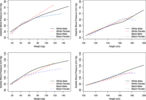
Figure 1: Marginal effects of weight and height on blood pressure using a LOWESS smoother.

5.2 Model specification

The following model is used to examine the joint height–weight effects on diastolic and systolic blood pressure in children:

$$\cases{\displaystyle\operatorname{DBP}_{ij}=U^{d}_{i}+p_{ij}\psi_{d}+\sum_{g=1}^{4}f^{d}_{g}(w_{ij},h_{ij})z_{ig}+\epsilon_{ij}^{d},\vspace*{2pt}\cr\displaystyle\operatorname{SBP}_{ij}=U^{s}_{i}+p_{ij}\psi_{s}+\sum_{g=1}^{4}f^{s}_{g}(w_{ij},h_{ij})z_{ig}+\epsilon_{ij}^{s},}$$ (7)

where $\operatorname{DBP}_{ij}$, $\operatorname{SBP}_{ij}$, $p_{ij}$, $w_{ij}$ and $h_{ij}$, respectively, represent the diastolic and systolic blood pressure, heart rate (or pulse, which is used as a surrogate marker for cardiac output), weight and height measured from the $i$th subject at the $j$th visit; $U^{d}_{i}$ and $U^{s}_{i}$ are the random subject effects; $\psi_{d}$ and $\psi_{s}$ are the regression coefficient parameters of heart rate on diastolic and systolic blood pressure respectively; $f^{d}_{g}$ and $f^{s}_{g}$ are the unknown bivariate smooth functions to depict the joint weight and height effects on diastolic and systolic blood pressure, respectively, in the four sex–ethnicity groups ($g=1,\dots,4$); and $z_{ig}$ is the corresponding group indicator. Note that the intercept terms $(\beta_{10},\ldots,\beta_{40})$ and $(\gamma_{10},\ldots,\gamma_{40})$ representing, respectively, the population average diastolic and systolic blood pressure in different sex–ethnicity groups are absorbed into the corresponding group-specific smooth components. The effects of heart rate were found to be linear in preliminary analyses. Hence, they are included in the model as linear components for ease of clinical interpretation. The random subject effects are assumed to have the same distribution as specified in model (1).

Since the outcomes are measured repeatedly for each subject during the follow-up, possible serial correlations may exist. According to the study protocol, enrolled subjects were asked to return every six months for measurements after the baseline screening. However, the longitudinal data collection was not exactly evenly spaced due to delayed or even missed clinic visits. To accommodate, we incorporate a continuous time autoregressive structure into the within-subject errors. To be more exact, we assume that $\operatorname{cor}(\epsilon_{ij}^{d},\epsilon_{ij^{\prime}}^{d})=\operatorname{cor}(\epsilon_{ij}^{s},\epsilon_{ij^{\prime}}^{s})=\phi^{|\mathit{age}_{ij}-\mathit{age}_{ij^{\prime}}|}$, for $1\leq j\neq j^{\prime}\leq n_{i}$, $i=1,\ldots,m$, where $\mathit{age}_{ij}$ denotes the age (in years) of subject $i$ at the $j$th visit and $\phi$ is the autocorrelation parameter of unit time interval.

The core model fitting procedure is based on the gamm (generalized additive mixed model) routine in R package mgcv [Wood (2010)]. We have made necessary extensions to accommodate the complex model features (e.g., correlation structure of paired longitudinal outcomes) and visualization of the results. The confidence intervals of the model parameters are derived from the observed information matrix in the LMM framework. The estimated bivariate smooth functions of weight and height in each sex–ethnicity group are presented and compared using colored image plots and contour lines. A detailed description of the model-fitting algorithms can be found in Section A of the supplementary materials [Liu and Tu (2012)], together with model diagnostics for model assumption verification and goodness-of-fit assessment in Section B.

5.3 Analytical results

From the REML estimates (which are very close to the ML estimates) of the semiparametric mixed model (7) based on 6867 pairs of blood pressure assessments from 418 subjects, we note a substantial correlation ($\widehat{\rho}=0.52$ with 95% confidence interval (CI) $[0.42,0.61]$) between the diastolic and systolic blood pressure within the same subject. Systolic blood pressure has slightly greater variability ($\widehat{\sigma}_{2}=5.29;$ 95% CI: $[4.88,5.73]$) than diastolic measurements ($\widehat{\sigma}_{1}=4.57;$ 95% CI: $[4.18,4.99]$), but the difference is not statistically significant. However, the random error associated with systolic blood pressure (within the same subject) has a significantly smaller variance, as reflected by the magnitude and corresponding confidence interval of the scaling parameter ($\widehat{\delta}=0.87;$ 95% CI: $[0.85,0.90]$). Such an observation is consistent with the previously published data on pediatric blood pressure measurements [Falkner et al. (2006)], and it may in part reflect the difficulty in clearly pinpointing the start of the fifth Korotkoff sound in diastolic measurement [Pickering et al. (2005)]. The estimated variance of the random error is $\widehat{\sigma}_{\epsilon}=7.39$; 95% CI: $[7.26,7.53]$. We also detected slight autocorrelation in within-subject errors, with $\widehat{\phi}=0.014;$ 95% CI: $[0.010,0.020]$. The estimates of the average diastolic and systolic blood pressure in different gender and ethnicity groups in model (7) are listed in Table 2. Heart rate has a negative effect on the diastolic blood pressure with $\psi_{d}=-0.04$ [standard deviation (SD)${}={}$0.01], whereas it is positively associated with systolic blood pressure $\psi_{s}=0.07$ (SD${}={}$0.01). The finding is not surprising because heart rate directly reflects cardiac output, which typically increases with pulse pressure (systolic minus diastolic blood pressure). With pulse pressure relating systolic positively and diastolic negatively, one would expect systolic blood pressure to increase with heart rate and diastolic blood pressure to decrease with heart rate.

Table 2: Estimates of the parameters of the semiparametric joint blood pressure model with 95% lower (confidence) bound (LB) and upper (confidence) bound (UB)

Parameter	Sex–ethnicity group	Estimate	Std. Dev.	95% LB	95% UB
$\beta_{10}$	White male	0$64.99$	$0.98$	63.03	066.95
$\beta_{20}$	White female	0$66.02$	$0.99$	64.04	068.00
$\beta_{30}$	Black male	0$65.98$	$1.09$	63.80	068.16
$\beta_{40}$	Black female	0$65.76$	$1.21$	63.34	068.18
$\gamma_{10}$	White male	$100.41$	$0.92$	98.57	102.25
$\gamma_{20}$	White female	0$97.51$	$0.93$	95.65	099.37
$\gamma_{30}$	Black male	0$99.93$	$1.05$	97.83	102.03
$\gamma_{40}$	Black female	0$98.27$	$1.17$	95.93	100.61

The estimated bivariate smooth functions of weight and height in the four sex–ethnicity groups are plotted in Figures 2 and 3.

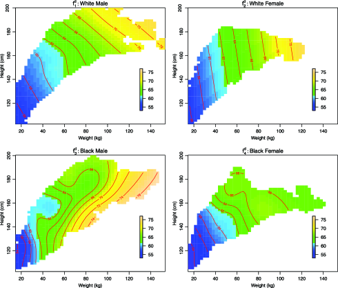
Figure 2: Bivariate smooth function estimates of the joint height–weight effects on diastolic blood pressure [defined in equation (7)] in boys and girls of different ethnicity.

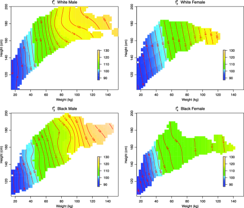
Figure 3: Bivariate smooth function estimates of the joint height–weight effects on systolic blood pressure [defined in equation (7)] in boys and girls of different ethnicity.

Both the adjusted likelihood ratio (LR) test [$2\log LR=217.6$ with reference distribution $(\chi^{2}_{84}+\chi^{2}_{85})/2$, $p<0.001$] and the bootstrap test (Figure 4 with $B=1000$ replications) suggest significantly different joint height–weight influences on blood pressure across the four sex and ethnicity groups. Aside from the significant test results of the bivariate height–weight effect surfaces, the most interesting observation from this analysis is the apparently different shape of these bivariate functions: (1) While blood pressure generally increases with weight as well as height, weight clearly has a much greater overall influence on blood pressure. In fact, at a given weight level, the height effects are often minimal, as indicated by the (nearly) vertical contour lines. (2) Among the heavier boys (those with weight greater than 120 kg, e.g.), blacks appear to have higher systolic blood pressure than whites. The reverse is true for girls. From the fitted effect surfaces, we see that heavier white girls appear to have higher systolic blood pressure than their black counterparts. (3) For diastolic blood pressure, while weight is still the dominant influence, height does have an effect. The more intriguing observation is perhaps the clear difference between black and white boys. For example, when weight is about 80 kg, taller black boys have lower diastolic blood pressure. While one would be attempted to attribute this to the lower corresponding BMI values, the opposite is true for white boys. These more complex pictures of height and weight influences on blood pressure point to possible existence of distinct physiology of blood pressure development in black and white children.

Figure 4: Empirical distribution of log-likelihood ratio based on bootstrap technique with $B=1000$ replications.

6 Discussion

In summary, we have presented a joint model for paired outcomes with bivariate effect surfaces of two continuous independent variables. This model extends previous work by accommodating longitudinally measured outcome pairs, as well as bivariate covariate effect surfaces. With the introduction of factor-by-surface interactions, it also allows for the incorporation of group-specific surfaces (i.e., group-height–weight interactions). For implementation, we have developed necessary computational procedures. Resampling-based and LRT-based inferences concerning the group-specific bivariate effects are discussed. Simulation study indicates adequate performances in the proposed adjusted LRT procedure.

Using the proposed method, we examined the influences of height and weight on blood pressure in children undergoing the pubertal growth process. For adults, there is a generally accepted notion that body weight has a predominant influence on blood pressure. For children that undergo the pubertal growth process, height and weight are known to increase concurrently with age, and both height and weight are positively related to blood pressure. Few studies have directly examined the relative contributions of height and weight, partly due to the lack of appropriate analytical tools to discern these simultaneous effects. With the newly developed statistical method, we examined the influences of height and weight on longitudinally measured blood pressure. We found that in children, just like in adults, weight tended to have a noticeably stronger impact on blood pressure, even during a period of vigorous linear growth. The study finding provides direct evidence that adiposity, as reflected by weight, is the primary driver of the blood pressure development in children. The finding is consistent with the latest pediatric literature on the connection between adiposity and blood pressure. Clinically, our finding highlights the importance of weight management in overweight and obese children: excessive weight gain could significantly increase the hypertension risk in children [Tu et al. (2011), Falkner and Gidding (2011)]. Mechanistically, weight-mediated blood pressure elevation in young and healthy children points to the need for studies focusing on including adipose-derived hormones. Animal and human studies suggested one of such hormones, leptin, could act upon the sympathetic nervous system (SNS), which contributes to the elevation of blood pressure. More recently, investigators have proposed mouse models describing new signaling pathways in the pathogenesis of obesity hypertension through leptin [Purkayastha, Zhang and Cai (2011), Humphreys (2011)]. Interestingly, in a separate investigation, our research team has also discovered dramatically increased leptin levels and heart rate (as an indicator for a more activated SNS) in overweight and obese children, corresponding to the elevated blood pressure [Tu et al. (2011)]. The findings from the current study certainly gives more credence to this hypothesized pathway between adiposity and blood pressure. We are currently investigating the possibility of adiposity acting upon blood pressure through alternative pathways, such as the renin-angiotensin-aldosterone system.

A limitation of this research is that we only included children who had ten or more longitudinal assessments in this methodological development, following a condition stipulated by our current data use agreement. While such a restriction could potentially limit the generalizability of the study finding, we note that the number of assessments is not related to the study subjects’ behaviors but to the timing of their school’s participation into the original study. As a result, children who had fewer assessments (and thus were excluded from the current analysis) are unlikely to be systematically different from those who contributed more observations. Notwithstanding this limitation, our research does provide an important analytical tool that may significantly enhance mechanistic and epidemiologic investigations concerning blood pressure development in children.

References

- Anderson and Whitaker (2009) {barticle}[author] \bauthor\bsnmAnderson, \bfnmS. E.\binitsS. E. and \bauthor\bsnmWhitaker, \bfnmR. C.\binitsR. C. (\byear2009). \btitlePrevalence of obesity among US preschool children in different racial and ethnic groups. \bjournalArchives of Pediatrics & Adolescent Medicine \bvolume163 \bpages344–348. \bptokimsref \endbibitem
- Baker, Olsen and Sorensen (2007) {barticle}[author] \bauthor\bsnmBaker, \bfnmJ. L.\binitsJ. L., \bauthor\bsnmOlsen, \bfnmL. W.\binitsL. W. and \bauthor\bsnmSorensen, \bfnmTIA\binitsT. (\byear2007). \btitleChildhood body-mass index and the risk of coronary heart disease in adulthood. \bjournalNew England Journal of Medicine \bvolume357 \bpages2329–2337. \bptokimsref \endbibitem
- Brady et al. (2010) {barticle}[pbm] \bauthor\bsnmBrady, \bfnmTammy M.\binitsT. M., \bauthor\bsnmFivush, \bfnmBarbara\binitsB., \bauthor\bsnmParekh, \bfnmRulan S.\binitsR. S. and \bauthor\bsnmFlynn, \bfnmJoseph T.\binitsJ. T. (\byear2010). \btitleRacial differences among children with primary hypertension. \bjournalPediatrics \bvolume126 \bpages931–937. \biddoi=10.1542/peds.2009-2972, issn=1098-4275, pii=peds.2009-2972, pmid=20956429 \bptokimsref \endbibitem
- Brezger, Fahrmeir and Hennerfeind (2007) {barticle}[mr] \bauthor\bsnmBrezger, \bfnmA.\binitsA., \bauthor\bsnmFahrmeir, \bfnmL.\binitsL. and \bauthor\bsnmHennerfeind, \bfnmA.\binitsA. (\byear2007). \btitleAdaptive Gaussian Markov random fields with applications in human brain mapping. \bjournalJ. Roy. Statist. Soc. Ser. C \bvolume56 \bpages327–345. \biddoi=10.1111/j.1467-9876.2007.00580.x, issn=0035-9254, mr=2370993 \bptokimsref \endbibitem
- Cleveland (1979) {barticle}[mr] \bauthor\bsnmCleveland, \bfnmWilliam S.\binitsW. S. (\byear1979). \btitleRobust locally weighted regression and smoothing scatterplots. \bjournalJ. Amer. Statist. Assoc. \bvolume74 \bpages829–836. \bidissn=0003-1291, mr=0556476 \bptokimsref \endbibitem
- Crainiceanu, Diggle and Rowlingson (2008) {barticle}[mr] \bauthor\bsnmCrainiceanu, \bfnmCiprian M.\binitsC. M., \bauthor\bsnmDiggle, \bfnmPeter J.\binitsP. J. and \bauthor\bsnmRowlingson, \bfnmBarry\binitsB. (\byear2008). \btitleBivariate binomial spatial modeling of Loa loa prevalence in tropical Africa. \bjournalJ. Amer. Statist. Assoc. \bvolume103 \bpages21–37. \biddoi=10.1198/016214507000001409, issn=0162-1459, mr=2420211 \bptnotecheck related\bptokimsref \endbibitem
- Crainiceanu and Ruppert (2004) {barticle}[mr] \bauthor\bsnmCrainiceanu, \bfnmCiprian M.\binitsC. M. and \bauthor\bsnmRuppert, \bfnmDavid\binitsD. (\byear2004). \btitleLikelihood ratio tests in linear mixed models with one variance component. \bjournalJ. R. Stat. Soc. Ser. B Stat. Methodol. \bvolume66 \bpages165–185. \biddoi=10.1111/j.1467-9868.2004.00438.x, issn=1369-7412, mr=2035765 \bptokimsref \endbibitem
- Davidson and Flachaire (2008) {barticle}[mr] \bauthor\bsnmDavidson, \bfnmRussell\binitsR. and \bauthor\bsnmFlachaire, \bfnmEmmanuel\binitsE. (\byear2008). \btitleThe wild bootstrap, tamed at last. \bjournalJ. Econometrics \bvolume146 \bpages162–169. \biddoi=10.1016/j.jeconom.2008.08.003, issn=0304-4076, mr=2459651 \bptokimsref \endbibitem
- Davy and Hall (2004) {barticle}[author] \bauthor\bsnmDavy, \bfnmK. P.\binitsK. P. and \bauthor\bsnmHall, \bfnmJ. E.\binitsJ. E. (\byear2004). \btitleObesity and hypertension: Two epidemics or one? \bjournalAmerican Journal of Physiology—Regulatory Integrative and Comparative Physiology \bvolume286 \bpagesR803–R813. \bptokimsref \endbibitem
- Dean, Nathoo and Nielsen (2007) {barticle}[mr] \bauthor\bsnmDean, \bfnmC. B.\binitsC. B., \bauthor\bsnmNathoo, \bfnmF.\binitsF. and \bauthor\bsnmNielsen, \bfnmJ. D.\binitsJ. D. (\byear2007). \btitleSpatial and mixture models for recurrent event processes. \bjournalEnvironmetrics \bvolume18 \bpages713–725. \biddoi=10.1002/env.870, issn=1180-4009, mr=2408940 \bptokimsref \endbibitem
- Dubin and Müller (2005) {barticle}[mr] \bauthor\bsnmDubin, \bfnmJoel A.\binitsJ. A. and \bauthor\bsnmMüller, \bfnmHans-Georg\binitsH.-G. (\byear2005). \btitleDynamical correlation for multivariate longitudinal data. \bjournalJ. Amer. Statist. Assoc. \bvolume100 \bpages872–881. \biddoi=10.1198/016214504000001989, issn=0162-1459, mr=2201015 \bptokimsref \endbibitem
- Falkner (2010) {barticle}[pbm] \bauthor\bsnmFalkner, \bfnmBonita\binitsB. (\byear2010). \btitleHypertension in children and adolescents: Epidemiology and natural history. \bjournalPediatr. Nephrol. \bvolume25 \bpages1219–1224. \biddoi=10.1007/s00467-009-1200-3, issn=1432-198X, pmcid=2874036, pmid=19421783 \bptokimsref \endbibitem
- Falkner and Gidding (2011) {barticle}[pbm] \bauthor\bsnmFalkner, \bfnmBonita\binitsB. and \bauthor\bsnmGidding, \bfnmSamuel\binitsS. (\byear2011). \btitleChildhood obesity and blood pressure: Back to the future? \bjournalHypertension \bvolume58 \bpages754–755. \biddoi=10.1161/HYPERTENSIONAHA.111.180430, issn=1524-4563, mid=NIHMS330276, pii=HYPERTENSIONAHA.111.180430, pmcid=3287055, pmid=21968756 \bptokimsref \endbibitem
- Falkner et al. (2006) {barticle}[pbm] \bauthor\bsnmFalkner, \bfnmBonita\binitsB., \bauthor\bsnmGidding, \bfnmSamuel S.\binitsS. S., \bauthor\bsnmRamirez-Garnica, \bfnmGabriela\binitsG., \bauthor\bsnmWiltrout, \bfnmStacey Armatti\binitsS. A., \bauthor\bsnmWest, \bfnmDavid\binitsD. and \bauthor\bsnmRappaport, \bfnmElizabeth B.\binitsE. B. (\byear2006). \btitleThe relationship of body mass index and blood pressure in primary care pediatric patients. \bjournalJ. Pediatr. \bvolume148 \bpages195–200. \biddoi=10.1016/j.jpeds.2005.10.030, issn=0022-3476, pii=S0022-3476(05)01002-4, pmid=16492428 \bptokimsref \endbibitem
- Fujita et al. (2010) {barticle}[pbm] \bauthor\bsnmFujita, \bfnmYuki\binitsY., \bauthor\bsnmKouda, \bfnmKatsuyasu\binitsK., \bauthor\bsnmNakamura, \bfnmHarunobu\binitsH., \bauthor\bsnmNishio, \bfnmNobuhiro\binitsN., \bauthor\bsnmTakeuchi, \bfnmHiroichi\binitsH. and \bauthor\bsnmIki, \bfnmMasayuki\binitsM. (\byear2010). \btitleRelationship between height and blood pressure in Japanese schoolchildren. \bjournalPediatr. Int. \bvolume52 \bpages689–693. \biddoi=10.1111/j.1442-200X.2010.03093.x, issn=1442-200X, pii=PED3093, pmid=20136723 \bptokimsref \endbibitem
- Ghosh and Hanson (2010) {barticle}[mr] \bauthor\bsnmGhosh, \bfnmPulak\binitsP. and \bauthor\bsnmHanson, \bfnmTimothy\binitsT. (\byear2010). \btitleA semiparametric Bayesian approach to multivariate longitudinal data. \bjournalAust. N. Z. J. Stat. \bvolume52 \bpages275–288. \biddoi=10.1111/j.1467-842X.2010.00581.x, issn=1369-1473, mr=2744574 \bptokimsref \endbibitem
- Ghosh and Tu (2009) {barticle}[mr] \bauthor\bsnmGhosh, \bfnmPulak\binitsP. and \bauthor\bsnmTu, \bfnmWanzhu\binitsW. (\byear2009). \btitleAssessing sexual attitudes and behaviors of young women: A joint model with nonlinear time effects, time varying covariates, and dropouts. \bjournalJ. Amer. Statist. Assoc. \bvolume104 \bpages474–485. \biddoi=10.1198/jasa.2009.0013, issn=0162-1459, mr=2751432 \bptokimsref \endbibitem
- Green and Silverman (1994) {bbook}[mr] \bauthor\bsnmGreen, \bfnmP. J.\binitsP. J. and \bauthor\bsnmSilverman, \bfnmB. W.\binitsB. W. (\byear1994). \btitleNonparametric Regression and Generalized Linear Models: A Roughness Penalty Approach. \bseriesMonographs on Statistics and Applied Probability \bvolume58. \bpublisherChapman & Hall, \baddressLondon. \bidmr=1270012 \bptokimsref \endbibitem
- Guillas and Lai (2010) {barticle}[mr] \bauthor\bsnmGuillas, \bfnmSerge\binitsS. and \bauthor\bsnmLai, \bfnmMing-Jun\binitsM.-J. (\byear2010). \btitleBivariate splines for spatial functional regression models. \bjournalJ. Nonparametr. Stat. \bvolume22 \bpages477–497. \biddoi=10.1080/10485250903323180, issn=1048-5252, mr=2662608 \bptokimsref \endbibitem
- Guo and Carlin (2004) {barticle}[mr] \bauthor\bsnmGuo, \bfnmXu\binitsX. and \bauthor\bsnmCarlin, \bfnmBradley P.\binitsB. P. (\byear2004). \btitleSeparate and joint modeling of longitudinal and event time data using standard computer packages. \bjournalAmer. Statist. \bvolume58 \bpages16–24. \biddoi=10.1198/0003130042854, issn=0003-1305, mr=2055507 \bptokimsref \endbibitem
- Hall (2003) {barticle}[pbm] \bauthor\bsnmHall, \bfnmJohn E.\binitsJ. E. (\byear2003). \btitleThe kidney, hypertension, and obesity. \bjournalHypertension \bvolume41 \bpages625–633. \biddoi=10.1161/01.HYP.0000052314.95497.78, issn=1524-4563, pii=01.HYP.0000052314.95497.78, pmid=12623970 \bptokimsref \endbibitem
- Hall et al. (2010) {barticle}[pbm] \bauthor\bsnmHall, \bfnmJohn E.\binitsJ. E., \bauthor\bparticleda \bsnmSilva, \bfnmAlexandre A.\binitsA. A., \bauthor\bparticledo \bsnmCarmo, \bfnmJussara M.\binitsJ. M., \bauthor\bsnmDubinion, \bfnmJohn\binitsJ., \bauthor\bsnmHamza, \bfnmShereen\binitsS., \bauthor\bsnmMunusamy, \bfnmShankar\binitsS., \bauthor\bsnmSmith, \bfnmGrant\binitsG. and \bauthor\bsnmStec, \bfnmDavid E.\binitsD. E. (\byear2010). \btitleObesity-induced hypertension: Role of sympathetic nervous system, leptin, and melanocortins. \bjournalJ. Biol. Chem. \bvolume285 \bpages17271–17276. \biddoi=10.1074/jbc.R110.113175, issn=1083-351X, pii=R110.113175, pmcid=2878489, pmid=20348094 \bptokimsref \endbibitem
- He, Fung and Zhu (2005) {barticle}[mr] \bauthor\bsnmHe, \bfnmXuming\binitsX., \bauthor\bsnmFung, \bfnmWing K.\binitsW. K. and \bauthor\bsnmZhu, \bfnmZhongyi\binitsZ. (\byear2005). \btitleRobust estimation in generalized partial linear models for clustered data. \bjournalJ. Amer. Statist. Assoc. \bvolume100 \bpages1176–1184. \biddoi=10.1198/016214505000000277, issn=0162-1459, mr=2236433 \bptokimsref \endbibitem
- Huang et al. (1998) {barticle}[author] \bauthor\bsnmHuang, \bfnmZ.\binitsZ., \bauthor\bsnmWillett, \bfnmW. C.\binitsW. C., \bauthor\bsnmManson, \bfnmJ. E.\binitsJ. E., \bauthor\bsnmRosner, \bfnmB.\binitsB., \bauthor\bsnmStampfer, \bfnmM. J.\binitsM. J., \bauthor\bsnmSpeizer, \bfnmF. E.\binitsF. E. and \bauthor\bsnmColditz, \bfnmG. A.\binitsG. A. (\byear1998). \btitleBody weight, weight change, and risk for hypertension in women. \bjournalAnnals of Internal Medicine \bvolume128 \bpages81–88. \bptokimsref \endbibitem
- Humphreys (2011) {barticle}[pbm] \bauthor\bsnmHumphreys, \bfnmMichael H.\binitsM. H. (\byear2011). \btitleThe brain splits obesity and hypertension. \bjournalNat. Med. \bvolume17 \bpages782–783. \biddoi=10.1038/nm0711-782, issn=1546-170X, pii=nm0711-782, pmid=21738154 \bptokimsref \endbibitem
- Jones (1993) {bbook}[mr] \bauthor\bsnmJones, \bfnmR. H.\binitsR. H. (\byear1993). \btitleLongitudinal Data with Serial Correlation: A State-Space Approach. \bseriesMonographs on Statistics and Applied Probability \bvolume47. \bpublisherChapman & Hall, \baddressLondon. \bidmr=1293123 \bptokimsref \endbibitem
- Kohn, Ansley and Tharm (1991) {barticle}[mr] \bauthor\bsnmKohn, \bfnmRobert\binitsR., \bauthor\bsnmAnsley, \bfnmCraig F.\binitsC. F. and \bauthor\bsnmTharm, \bfnmDavid\binitsD. (\byear1991). \btitleThe performance of cross-validation and maximum likelihood estimators of spline smoothing parameters. \bjournalJ. Amer. Statist. Assoc. \bvolume86 \bpages1042–1050. \bidissn=0162-1459, mr=1146351 \bptokimsref \endbibitem
- Lauer and Clarke (1989) {barticle}[pbm] \bauthor\bsnmLauer, \bfnmR. M.\binitsR. M. and \bauthor\bsnmClarke, \bfnmW. R.\binitsW. R. (\byear1989). \btitleChildhood risk factors for high adult blood pressure: The muscatine study. \bjournalPediatrics \bvolume84 \bpages633–641. \bidissn=0031-4005, pmid=2780125 \bptokimsref \endbibitem
- Lever and Harrap (1992) {barticle}[pbm] \bauthor\bsnmLever, \bfnmA. F.\binitsA. F. and \bauthor\bsnmHarrap, \bfnmS. B.\binitsS. B. (\byear1992). \btitleEssential hypertension: A disorder of growth with origins in childhood? \bjournalJ. Hypertens. \bvolume10 \bpages101–120. \bidissn=0263-6352, pmid=1313473 \bptokimsref \endbibitem
- Levin et al. (2010) {barticle}[pbm] \bauthor\bsnmLevin, \bfnmAvi\binitsA., \bauthor\bsnmMorad, \bfnmYair\binitsY., \bauthor\bsnmGrotto, \bfnmItamar\binitsI., \bauthor\bsnmRavid, \bfnmMordechai\binitsM. and \bauthor\bsnmBar-Dayan, \bfnmYosefa\binitsY. (\byear2010). \btitleWeight disorders and associated morbidity among young adults in Israel 1990–2003. \bjournalPediatr. Int. \bvolume52 \bpages347–352. \biddoi=10.1111/j.1442-200X.2009.02972.x, issn=1442-200X, pii=PED2972, pmid=19807878 \bptokimsref \endbibitem
- Lin and Carroll (2006) {barticle}[mr] \bauthor\bsnmLin, \bfnmXihong\binitsX. and \bauthor\bsnmCarroll, \bfnmRaymond J.\binitsR. J. (\byear2006). \btitleSemiparametric estimation in general repeated measures problems. \bjournalJ. R. Stat. Soc. Ser. B Stat. Methodol. \bvolume68 \bpages69–88. \biddoi=10.1111/j.1467-9868.2005.00533.x, issn=1369-7412, mr=2212575 \bptokimsref \endbibitem
- Lin and Zhang (1999) {barticle}[mr] \bauthor\bsnmLin, \bfnmXihong\binitsX. and \bauthor\bsnmZhang, \bfnmDaowen\binitsD. (\byear1999). \btitleInference in generalized additive mixed models by using smoothing splines. \bjournalJ. R. Stat. Soc. Ser. B Stat. Methodol. \bvolume61 \bpages381–400. \biddoi=10.1111/1467-9868.00183, issn=1369-7412, mr=1680318 \bptokimsref \endbibitem
- Liu (1988) {barticle}[mr] \bauthor\bsnmLiu, \bfnmRegina Y.\binitsR. Y. (\byear1988). \btitleBootstrap procedures under some non-i.i.d. models. \bjournalAnn. Statist. \bvolume16 \bpages1696–1708. \biddoi=10.1214/aos/1176351062, issn=0090-5364, mr=0964947 \bptokimsref \endbibitem
- Liu and Tu (2012) {bmisc}[author] \bauthor\bsnmLiu, \bfnmH.\binitsH. and \bauthor\bsnmTu, \bfnmW.\binitsW. (\byear2012). \bhowpublishedSupplement to “A semiparametric regression model for paired longitudinal outcomes with application in childhood blood pressure development.” DOI:\doiurl10.1214/12-AOAS567SUPP. \bptokimsref \endbibitem
- Mammen (1993) {barticle}[mr] \bauthor\bsnmMammen, \bfnmEnno\binitsE. (\byear1993). \btitleBootstrap and wild bootstrap for high-dimensional linear models. \bjournalAnn. Statist. \bvolume21 \bpages255–285. \biddoi=10.1214/aos/1176349025, issn=0090-5364, mr=1212176 \bptokimsref \endbibitem
- Masuo et al. (2000) {barticle}[pbm] \bauthor\bsnmMasuo, \bfnmK.\binitsK., \bauthor\bsnmMikami, \bfnmH.\binitsH., \bauthor\bsnmOgihara, \bfnmT.\binitsT. and \bauthor\bsnmTuck, \bfnmM. L.\binitsM. L. (\byear2000). \btitleWeight gain-induced blood pressure elevation. \bjournalHypertension \bvolume35 \bpages1135–1140. \bidissn=1524-4563, pmid=10818077 \bptokimsref \endbibitem
- Morris (2002) {barticle}[mr] \bauthor\bsnmMorris, \bfnmJeffrey S.\binitsJ. S. (\byear2002). \btitleThe BLUPs are not “best” when it comes to bootstrapping. \bjournalStatist. Probab. Lett. \bvolume56 \bpages425–430. \biddoi=10.1016/S0167-7152(02)00041-X, issn=0167-7152, mr=1898721 \bptokimsref \endbibitem
- Morris et al. (2001) {barticle}[mr] \bauthor\bsnmMorris, \bfnmJeffrey S.\binitsJ. S., \bauthor\bsnmWang, \bfnmNaisyin\binitsN., \bauthor\bsnmLupton, \bfnmJoanne R.\binitsJ. R., \bauthor\bsnmChapkin, \bfnmRobert S.\binitsR. S., \bauthor\bsnmTurner, \bfnmNancy D.\binitsN. D., \bauthor\bsnmHong, \bfnmMee Young\binitsM. Y. and \bauthor\bsnmCarroll, \bfnmRaymond J.\binitsR. J. (\byear2001). \btitleParametric and nonparametric methods for understanding the relationship between carcinogen-induced DNA adduct levels in distal and proximal regions of the colon. \bjournalJ. Amer. Statist. Assoc. \bvolume96 \bpages816–826. \biddoi=10.1198/016214501753208528, issn=0162-1459, mr=1946358 \bptokimsref \endbibitem
- Pickering et al. (2005) {barticle}[pbm] \bauthor\bsnmPickering, \bfnmThomas G.\binitsT. G., \bauthor\bsnmHall, \bfnmJohn E.\binitsJ. E., \bauthor\bsnmAppel, \bfnmLawrence J.\binitsL. J., \bauthor\bsnmFalkner, \bfnmBonita E.\binitsB. E., \bauthor\bsnmGraves, \bfnmJohn\binitsJ., \bauthor\bsnmHill, \bfnmMartha N.\binitsM. N., \bauthor\bsnmJones, \bfnmDaniel W.\binitsD. W., \bauthor\bsnmKurtz, \bfnmTheodore\binitsT., \bauthor\bsnmSheps, \bfnmSheldon G.\binitsS. G. and \bauthor\bsnmRoccella, \bfnmEdward J.\binitsE. J. (\byear2005). \btitleRecommendations for blood pressure measurement in humans and experimental animals: Part 1: Blood pressure measurement in humans: A statement for professionals from the Subcommittee of Professional and Public Education of the American Heart Association Council on High Blood Pressure Research. \bjournalHypertension \bvolume45 \bpages142–161. \biddoi=10.1161/01.HYP.0000150859.47929.8e, issn=1524-4563, pii=01.HYP.0000150859.47929.8e, pmid=15611362 \bptokimsref \endbibitem
- Pinheiro and Bates (2000) {bbook}[author] \bauthor\bsnmPinheiro, \bfnmJ. C.\binitsJ. C. and \bauthor\bsnmBates, \bfnmD. M.\binitsD. M. (\byear2000). \btitleMixed-Effects Models in S and S-PLUS. \bpublisherSpringer, \baddressNew York. \bptokimsref \endbibitem
- Purkayastha, Zhang and Cai (2011) {barticle}[pbm] \bauthor\bsnmPurkayastha, \bfnmSudarshana\binitsS., \bauthor\bsnmZhang, \bfnmGuo\binitsG. and \bauthor\bsnmCai, \bfnmDongsheng\binitsD. (\byear2011). \btitleUncoupling the mechanisms of obesity and hypertension by targeting hypothalamic IKK-beta and NF-kappa B. \bjournalNat. Med. \bvolume17 \bpages883–887. \biddoi=10.1038/nm.2372, issn=1546-170X, mid=NIHMS286510, pii=nm.2372, pmcid=3134198, pmid=21642978 \bptokimsref \endbibitem
- Roca-Pardiñas et al. (2008) {barticle}[mr] \bauthor\bsnmRoca-Pardiñas, \bfnmJavier\binitsJ., \bauthor\bsnmCadarso-Suárez, \bfnmCarmen\binitsC., \bauthor\bsnmTahoces, \bfnmPablo G.\binitsP. G. and \bauthor\bsnmLado, \bfnmMaría J.\binitsM. J. (\byear2008). \btitleAssessing continuous bivariate effects among different groups through nonparametric regression models: An application to breast cancer detection. \bjournalComput. Statist. Data Anal. \bvolume52 \bpages1958–1970. \biddoi=10.1016/j.csda.2007.06.024, issn=0167-9473, mr=2418483 \bptokimsref \endbibitem
- Ruppert, Wand and Carroll (2003) {bbook}[mr] \bauthor\bsnmRuppert, \bfnmDavid\binitsD., \bauthor\bsnmWand, \bfnmM. P.\binitsM. P. and \bauthor\bsnmCarroll, \bfnmR. J.\binitsR. J. (\byear2003). \btitleSemiparametric Regression. \bseriesCambridge Series in Statistical and Probabilistic Mathematics \bvolume12. \bpublisherCambridge Univ. Press, \baddressCambridge. \biddoi=10.1017/CBO9780511755453, mr=1998720 \bptokimsref \endbibitem
- Sain et al. (2006) {barticle}[author] \bauthor\bsnmSain, \bfnmS. R.\binitsS. R., \bauthor\bsnmJagtap, \bfnmS.\binitsS., \bauthor\bsnmMearns, \bfnmL.\binitsL. and \bauthor\bsnmNychka, \bfnmD.\binitsD. (\byear2006). \btitleA multivariate spatial model for soil water profiles. \bjournalJ. Agric. Biol. Environ. Stat. \bvolume11 \bpages462–480. \bptokimsref \endbibitem
- Self and Liang (1987) {barticle}[mr] \bauthor\bsnmSelf, \bfnmSteven G.\binitsS. G. and \bauthor\bsnmLiang, \bfnmKung-Yee\binitsK.-Y. (\byear1987). \btitleAsymptotic properties of maximum likelihood estimators and likelihood ratio tests under nonstandard conditions. \bjournalJ. Amer. Statist. Assoc. \bvolume82 \bpages605–610. \bidissn=0162-1459, mr=0898365 \bptokimsref \endbibitem
- Shankar et al. (2005) {barticle}[author] \bauthor\bsnmShankar, \bfnmR. R.\binitsR. R., \bauthor\bsnmEckert, \bfnmG. J.\binitsG. J., \bauthor\bsnmSaha, \bfnmC.\binitsC., \bauthor\bsnmTu, \bfnmW.\binitsW. and \bauthor\bsnmPratt, \bfnmJ. H.\binitsJ. H. (\byear2005). \btitleThe change in blood pressure during pubertal growth. \bjournalJournal of Clinical Endocrinology & Metabolism \bvolume90 \bpages163–167. \bptokimsref \endbibitem
- Steinberger et al. (2009) {barticle}[author] \bauthor\bsnmSteinberger, \bfnmJ.\binitsJ., \bauthor\bsnmDaniels, \bfnmS. R.\binitsS. R., \bauthor\bsnmEckel, \bfnmR. H.\binitsR. H., \bauthor\bsnmHayman, \bfnmL.\binitsL., \bauthor\bsnmLustig, \bfnmR. H.\binitsR. H., \bauthor\bsnmMcCrindle, \bfnmB.\binitsB. and \bauthor\bsnmMietus-Snyder, \bfnmM. L.\binitsM. L. (\byear2009). \btitleProgress and challenges in metabolic syndrome in children and adolescents: A scientific statement from the American Heart Association atherosclerosis, hypertension, and obesity in the young Committee of the Council on cardiovascular disease in the young; Council on cardiovascular nursing; and Council on nutrition, physical activity, and metabolism. \bjournalCirculation \bvolume119 \bpages628–647. \bptokimsref \endbibitem
- Stram and Lee (1994) {barticle}[author] \bauthor\bsnmStram, \bfnmD. O.\binitsD. O. and \bauthor\bsnmLee, \bfnmJ. W.\binitsJ. W. (\byear1994). \btitleVariance-components testing in the longitudinal mixed effects model. \bjournalBiometrics \bvolume50 \bpages1171–1177. \bptokimsref \endbibitem
- Stray-Pedersen et al. (2009) {barticle}[pbm] \bauthor\bsnmStray-Pedersen, \bfnmMarit\binitsM., \bauthor\bsnmHelsing, \bfnmRagnhild M.\binitsR. M., \bauthor\bsnmGibbons, \bfnmLuz\binitsL., \bauthor\bsnmCormick, \bfnmGabriela\binitsG., \bauthor\bsnmHolmen, \bfnmTurid L.\binitsT. L., \bauthor\bsnmVik, \bfnmTorstein\binitsT. and \bauthor\bsnmBelizán, \bfnmJosé M.\binitsJ. M. (\byear2009). \btitleWeight status and hypertension among adolescent girls in Argentina and Norway: Data from the ENNyS and HUNT studies. \bjournalBMC Public Health \bvolume9 \bpages398. \biddoi=10.1186/1471-2458-9-398, issn=1471-2458, pii=1471-2458-9-398, pmcid=2775744, pmid=19878550 \bptokimsref \endbibitem
- Tu et al. (2009) {barticle}[author] \bauthor\bsnmTu, \bfnmW.\binitsW., \bauthor\bsnmEckert, \bfnmG. J.\binitsG. J., \bauthor\bsnmSaha, \bfnmC.\binitsC. and \bauthor\bsnmPratt, \bfnmJ. H.\binitsJ. H. (\byear2009). \btitleSynchronization of adolescent blood pressure and pubertal somatic growth. \bjournalJournal of Clinical Endocrinology & Metabolism \bvolume94 \bpages5019–5022. \bptokimsref \endbibitem
- Tu et al. (2011) {barticle}[author] \bauthor\bsnmTu, \bfnmW\binitsW., \bauthor\bsnmEckert, \bfnmG. J.\binitsG. J., \bauthor\bsnmDiMeglio, \bfnmL. A.\binitsL. A., \bauthor\bsnmYu, \bfnmZ.\binitsZ., \bauthor\bsnmJung, \bfnmJ.\binitsJ. and \bauthor\bsnmPratt, \bfnmJ. H.\binitsJ. H. (\byear2011). \btitleIntensified effect of adiposity on blood pressure in overweight and obese children. \bjournalHypertension \bvolume58 \bpages818–824. \bptokimsref \endbibitem
- Wahba (1985) {barticle}[mr] \bauthor\bsnmWahba, \bfnmGrace\binitsG. (\byear1985). \btitleA comparison of GCV and GML for choosing the smoothing parameter in the generalized spline smoothing problem. \bjournalAnn. Statist. \bvolume13 \bpages1378–1402. \biddoi=10.1214/aos/1176349743, issn=0090-5364, mr=0811498 \bptokimsref \endbibitem
- Wood (2003) {barticle}[mr] \bauthor\bsnmWood, \bfnmSimon N.\binitsS. N. (\byear2003). \btitleThin plate regression splines. \bjournalJ. R. Stat. Soc. Ser. B Stat. Methodol. \bvolume65 \bpages95–114. \biddoi=10.1111/1467-9868.00374, issn=1369-7412, mr=1959095 \bptokimsref \endbibitem
- Wood (2006) {bbook}[mr] \bauthor\bsnmWood, \bfnmSimon N.\binitsS. N. (\byear2006). \btitleGeneralized Additive Models: An Introduction with . \bpublisherChapman & Hall/CRC, \baddressBoca Raton, FL. \bidmr=2206355 \bptokimsref \endbibitem
- Wood (2010) {bmisc}[author] \bauthor\bsnmWood, \bfnmS. N.\binitsS. N. (\byear2010). \bhowpublishedmgcv: GAMs with GCV/AIC/REML smoothness estimation and GAMMs by PQL. R package version 1.7-2. \bptokimsref \endbibitem
- Zhang and Lin (2003) {barticle}[author] \bauthor\bsnmZhang, \bfnmD.\binitsD. and \bauthor\bsnmLin, \bfnmX.\binitsX. (\byear2003). \btitleHypothesis testing in semiparametric additive mixed models. \bjournalBiostatistics \bvolume4 \bpages57–74. \bptokimsref \endbibitem