Quantum walks with memory on cycles

Abstract

We study the model of quantum walks on cycles enriched by the addition of 1-step memory. We provide a formula for the probability distribution and the time-averaged limiting probability distribution of the introduced quantum walk. Using the obtained results, we discuss the properties of the introduced model and the difference in comparison to the memoryless model.

I Introduction

During the last few years a considerable research effort has been made to develop new algorithms based on the rules of quantum mechanics. Among the methods used to achieve this goal, quantum walks, a quantum counterpart of random walks, provide one of the most promising and successful approaches.

Classical random walks can be applied to solve many computational problems. They are used, for example, to find spanning trees and shortest paths in graphs, to find the convex hull of a set of points or to provide a sampling-based volume estimation reitzner12walks . Today a huge research effort is devoted to applying random walks in different areas of science. Classical random walks find their application in a plethora of areas. This has motivated big interest in using a similar model for developing algorithms which could harness the possibilities offered by quantum machines.

Quantum walks are counterparts of classical random walks governed by the rules of quantum mechanics venegas08synthesis ; vanegas12review ; reitzner12walks and provide a promising method for developing new quantum algorithms. Among the applications of quantum walks one can point out: solving the element distinctness ambainis07distinctness and subset finding childs05subset problems, spatial search childs04spatial , triangle finding magniez05quantum and verifying matrix products buhrman06quantum . The survey of quantum algorithms based on quantum walks is presented in ambainis03algorithmic .

The influence of memory on the behavior of quantum walks has been considered by Flitney et al. flitney04quantum and Brun et al. brun03quantum . In mcgettrick10one Mc Gettrick proposed a model of one-dimensional quantum walk on line with one-step memory and studied the limiting probability distribution for this model. This work was developed by Konno and Machida in konno10limit . More recently Rohde et al. considered a quantum walk with memory constructed using recycled coins and applied numerical experiments to study its properties. Moreover, an experimental proposal for implementing a quantum walk with memory using linear optics has also been considered in rohde12quantum .

In this paper we introduce and study the model of quantum walks on cycle aharonov01walks ; bednarska03walks enriched by the addition of 1-step memory mcgettrick10one . Our main contribution is the calculation of the probability of finding the particle at each position after given number of steps, and the limiting probability distribution for the introduced model. We also point out the differences between quantum walks on cycles with and without memory.

This paper is organized as follows. In Section II we introduce the model of a quantum walk on cycle with one-step memory. In Section III we analyze the introduced model using Fourier transform method and we discuss the behavior of the time-averaged limiting probability distribution of the discussed model. Finally, in Section IV we summarize the obtained results and provide some concluding remarks.

II The model

In the model discussed in bednarska03walks the space used by a quantum walk is composed of two parts – 1-qubit coin and $d$-dimensional state space, i.e. $\mathcal{H}=\mathcal{H}_{2}\otimes\mathcal{H}_{d}$. The shift operator in this case is defined as

$$S_{0}=\sum_{c=0}^{1}\sum_{v=0}^{d-1}|c\rangle\langle c|\otimes|v+2c-1\bmod d\rangle\langle v|.$$ (1)

Here we adopt this model and extend it with an additional register, referred to as memory register, which stores the history of a walk.

For a quantum walk with one step memory one needs a single qubit to store the history. In this case we use a Hilbert space of the form $\mathcal{H}=\mathcal{H}^{c}_{2}\otimes\mathcal{H}^{\mathrm{m}}_{2}\otimes\mathcal{H}_{d}$, respectively for a coin, memory and a position.

As in the case of a memoryless walk, the first register is the coin register and the third register is used to encode the position of the particle. The second register stores the history of the walk. The history is encoded as direction from which the particle was moved in the previous move. If this register is in the state $|0\rangle$, the previous position of the particle was $n+1$. If this register is in the state $|1\rangle$, the previous position of the particle was $n-1$. The coin register indicates if the walk should continue in the previously chosen direction (transmission in state $|0\rangle$) or change the direction (reflection in state $|1\rangle$).

Taking into account the above, we define a shift operator for a quantum walk with a 1-step memory on cycle with $d$ nodes as

$$\begin{split}S_{1}=\sum_{n=0}^{d-1}&\Big{(}|0\rangle\langle 0|\otimes|0,n-1(\bmod d)\rangle\langle 0,n|\\ +&|0\rangle\langle 0|\otimes|1,n+1(\bmod d)\rangle\langle 1,n|\\ +&|1\rangle\langle 1|\otimes|1,n+1(\bmod d)\rangle\langle 0,n|\\ +&|1\rangle\langle 1|\otimes|0,n-1(\bmod d)\rangle\langle 1,n|\Big{)},\end{split}$$ (2)

or in a more consistent form as

$$S_{1}=\sum_{n,m,c}|c\rangle\langle c|\otimes|h_{m,c},n+2h_{m,c}-1(\bmod d)\rangle\langle m,n|,$$ (3)

where $h_{m,c}=m+c(\bmod 2)$ represents a history dependence of the walk.

The walk operator is defined as toss-a-coin and make-a-move combination, i.e.

$$W_{1}=S_{1}(C\otimes{\rm 1l}_{2}\otimes{\rm 1l}_{d}),$$ (4)

where $C$ is a coin matrix, e.g. Hadamard matrix $H$

$$H=\frac{1}{\sqrt{2}}\left(\begin{matrix}1&1\\ 1&-1\end{matrix}\right)$$ (5)

or any matrix $C\in\mathrm{SU}(2)$.

The walk starts in some initial state $|\phi_{0}\rangle$. After each step the state is changed according to the formula

$$|\phi_{n}\rangle=W_{1}^{n}|\phi_{0}\rangle$$ (6)

or as a recursive relation

$$|\phi_{n+1}\rangle=W_{1}|\phi_{n}\rangle.$$ (7)

The probability of finding a particle at position $v$ after $n$ steps is obtained after averaging over the coin and the memory registers

$$p(v,n)=\sum_{c,m}|\langle{c,m,v}|{\phi_{n}}\rangle|^{2},$$ (8)

or, in other words, by tracing out over the memory and the coin subspaces

$$p(v,n)=\operatorname{tr}_{c,m}|\phi_{n}\rangle\langle\phi_{n}|,$$ (9)

where $\operatorname{tr}_{c,m}$ denotes the operation of tracing out with respect to the coin and the memory subspaces.

In aharonov01walks it was shown that $p(v,n)$ is quasi-periodic for memoryless walks on cycles and it was suggested to consider quantity

$$\bar{p}(n,t)=\frac{1}{t}\sum_{s=1}^{t}p(n,s),$$ (10)

which converges with $t\rightarrow\infty$ to the limiting distribution $p(v)$. As the parameter $n$ in this formula corresponds to the time required to perform $n$ steps, we refer to so defined $\bar{p}(v)$ as time-averaged limiting distribution.

III Probability distribution

In what follows we evaluate the probability distribution of finding the particle at each node of the cycle. We consider the Hadamard walk only. Thus the walk operator is given as

$$W=S(H\otimes{\rm 1l}_{2d}).$$ (11)

The second factor in the Eq. (11) can be written in the matrix notation as

$$H\otimes{\rm 1l}_{2d}=\frac{1}{\sqrt{2}}\left(\begin{matrix}{\rm 1l}_{2d}&{\rm 1l}_{2d}\\ {\rm 1l}_{2d}&-{\rm 1l}_{2d}\\ \end{matrix}\right).$$ (12)

III.1 Fourier analysis

In order to obtain expression for the probability distribution on the cycle we use Fourier analysis method nayak00line ; grimmett04waek ; konno10limit .

Below we calculate amplitudes for a walk on cycle with a 1-step memory with the Hadamard matrix acting on the coin register. In this case we represent the vectors of amplitudes as

$$\Phi(n,t)=\left(\begin{matrix}\langle{0,0,n}|{\psi_{t}}\rangle\\ \langle{0,1,n}|{\psi_{t}}\rangle\\ \langle{1,0,n}|{\psi_{t}}\rangle\\ \langle{1,1,n}|{\psi_{t}}\rangle\end{matrix}\right).$$ (13)

The shift operator is defined as in Eq. (2). In this case the interesting part of the shift operator reads

$$\begin{split}S_{1}(n)&=|0\rangle\langle 0|\otimes|0,n\rangle\langle 0,n+1|+|0\rangle\langle 0|\otimes|1,n\rangle\langle 1,n-1|\\ &+|1\rangle\langle 1|\otimes|0,n\rangle\langle 1,n+1|+|1\rangle\langle 1|\otimes|1,n\rangle\langle 0,n-1|\end{split}.$$ (14)

After one step of time evolution we have

$$\Phi(n,t+1)=\left(\begin{matrix}\langle 0,0,n+1|(H\otimes{\rm 1l}_{2}\otimes{\rm 1l}_{d})|\psi_{t}\rangle\\ \langle 0,1,n-1|(H\otimes{\rm 1l}_{2}\otimes{\rm 1l}_{d})|\psi_{t}\rangle\\ \langle 1,1,n+1|(H\otimes{\rm 1l}_{2}\otimes{\rm 1l}_{d})|\psi_{t}\rangle\\ \langle 1,0,n-1|(H\otimes{\rm 1l}_{2}\otimes{\rm 1l}_{d})|\psi_{t}\rangle\end{matrix}\right).$$

Evaluating the action of the Hadamard gate on the coin register one gets

$$\Phi(n,t+1) =\frac{1}{\sqrt{2}}\left(\begin{smallmatrix}\langle{0,0,n+1}|{\psi_{t}}\rangle+\langle{1,0,n+1}|{\psi_{t}}\rangle\\ 0\\ \langle{0,1,n+1}|{\psi_{t}}\rangle-\langle{1,1,n+1}|{\psi_{t}}\rangle\\ 0\end{smallmatrix}\right)$$

$$+\frac{1}{\sqrt{2}}\left(\begin{smallmatrix}0\\ \langle{0,1,n-1}|{\psi_{t}}\rangle+\langle{1,1,n-1}|{\psi_{t}}\rangle\\ 0\\ \langle{0,0,n-1}|{\psi_{t}}\rangle-\langle{1,0,n-1}|{\psi_{t}}\rangle\end{smallmatrix}\right).$$

Rewriting the above expression using $\Phi(n+1,t)$ and $\Phi(n-1,t)$ one gets

$$\Phi(n,t+1)=M_{-}\Phi(n+1,t)+M_{+}\Phi(n-1,t),$$ (15)

where $M_{+}$ (advancing) and $M_{-}$ (retarding) matrices read

$$M_{+} = \frac{1}{\sqrt{2}}\left(\begin{smallmatrix}0&0&0&0\\ 0&1&0&1\\ 0&0&0&0\\ 1&0&-1&0\end{smallmatrix}\right),$$ (16)

$$M_{-} = \frac{1}{\sqrt{2}}\left(\begin{smallmatrix}1&0&1&0\\ 0&0&0&0\\ 0&1&0&-1\\ 0&0&0&0\end{smallmatrix}\right).$$ (17)

In order to obtain the expression for the amplitudes of the quantum walk with memory on cycle we use the method introduced in nayak00line and represent time evolution of the walk using the Fourier transform

$$\tilde{\Phi}(k,t+1) = \sum_{n=0}^{d-1}e^{2\pi ikn/d}\Phi(n,t+1)$$

$$= \sum_{n=0}^{d-1}e^{2\pi ikn/d}(M_{-}\Phi(n+1,t)+M_{+}\Phi(n-1,t))$$

$$= \left(e^{-2\pi ikn/d}M_{-}+e^{2\pi ikn/d}M_{+}\right)\tilde{\Phi}(k,t).$$

From the above we get a recursive relation for the time evolution in the Fourier basis

$$\tilde{\Phi}(k,t)=M_{k}^{t}\tilde{\Phi}(k,0),$$ (19)

where

$$M_{k}=\frac{1}{\sqrt{2}}\left(\begin{array}[]{cccc}e^{-\frac{2ik\pi}{d}}&0&e^{-\frac{2ik\pi}{d}}&0\\ 0&e^{\frac{2ik\pi}{d}}&0&e^{\frac{2ik\pi}{d}}\\ 0&e^{-\frac{2ik\pi}{d}}&0&-e^{-\frac{2ik\pi}{d}}\\ e^{\frac{2ik\pi}{d}}&0&-e^{\frac{2ik\pi}{d}}&0\end{array}\right).$$ (20)

Let us now denote $A=\exp(-2\pi ik/d)$. Matrix $M_{k}$ has the following eigenvalues

$$\lambda_{1} = -1,$$

$$\lambda_{2} = 1,$$

$$\lambda_{3} = \frac{1+A^{2}+\sqrt{A^{4}-6A^{2}+1}}{2\sqrt{2}A},$$

$$\lambda_{4} = \frac{1+A^{2}-\sqrt{A^{4}-6A^{2}+1}}{2\sqrt{2}A},$$

with corresponding (orthonogal, but unnormalized) eigenvectors

$$v_{1} = \left\{\begin{smallmatrix}-\frac{\sqrt{2}A^{2}}{2A+\sqrt{2}}\\ -\frac{1}{\sqrt{2}A+1}\\ \frac{A\left(\sqrt{2}A+2\right)}{2A+\sqrt{2}}\\ 1\end{smallmatrix}\right\},\quad v_{2}=\left\{\begin{smallmatrix}\frac{A^{2}}{\sqrt{2}A-1}\\ \frac{1}{\sqrt{2}A-1}\\ \frac{A\left(\sqrt{2}A-2\right)}{\sqrt{2}-2A}\\ 1\end{smallmatrix}\right\},$$

$$v_{3} = \left\{\begin{smallmatrix}\frac{1}{2}\left(A^{2}-\sqrt{A^{4}-6A^{2}+1}-1\right)\\ \frac{A^{2}+\sqrt{A^{4}-6A^{2}+1}-1}{2A^{2}}\\ -1\\ 1\end{smallmatrix}\right\},$$

$$v_{4} = \left\{\begin{smallmatrix}\frac{1}{2}\left(A^{2}+\sqrt{A^{4}-6A^{2}+1}-1\right)\\ -\frac{-A^{2}+\sqrt{A^{4}-6A^{2}+1}+1}{2A^{2}}\\ -1\\ 1\end{smallmatrix}\right\}.$$

III.2 Initial state and time evolution

In order to evaluate the probability distribution we need to choose the initial state of the walk. Again following nayak00line we start from the position $0$ with the coin in the state $|0\rangle$. As in this case we have extra register for storing memory, in the initial state the state vector reads

$$|\phi_{0}\rangle=\frac{1}{\sqrt{2}}\left(\begin{smallmatrix}1\\ 1\\ 0\\ 0\end{smallmatrix}\right)\otimes|0\rangle,$$ (21)

which means that the memory register is in the superposition $\frac{1}{\sqrt{2}}(|0\rangle+|1\rangle)$ and the coin register is in the state $|0\rangle$.The vector of amplitudes in this situation reads

$$\Phi(n,0)=\frac{1}{\sqrt{2}}\left(\begin{smallmatrix}1\\ 1\\ 0\\ 0\end{smallmatrix}\right)\delta_{n0}.$$ (22)

Thus in the Fourier basis we start from the state

$$\tilde{\Phi}(k,0)=\frac{1}{\sqrt{2}}\left(\begin{smallmatrix}1\\ 1\\ 0\\ 0\end{smallmatrix}\right),$$ (23)

for any $k=0,\ldots,d-1$.

III.3 Initial state decomposition

Using the eigendecomposition of the matrix $M_{k}$ we can calculate the form of the amplitudes in the Fourier basis after $t$ steps. After $t$ steps the vector of the amplitudes reads

$$\tilde{\Phi}(k,t)=M_{k}^{t}\tilde{\Phi}(k,0)=M_{k}^{t}\frac{1}{\sqrt{2}}\left(\begin{smallmatrix}1\\ 1\\ 0\\ 0\end{smallmatrix}\right)$$ (24)

for any $k$.

Let us now write the initial state of the walk $\tilde{\Phi}(k,0)$ in the $\{v_{i}\}_{i=1,\dots,4}$ basis as

$$\tilde{\Phi}(k,0)=\sum_{i=1}^{4}\alpha_{i}(k)v_{i}(k).$$ (25)

where

$$\alpha_{i}(k)=(v_{i}(k),\tilde{\Phi}(k,0))$$ (26)

are components of $\tilde{\Phi}(k,0)$ in $\{v_{i}\}_{i=1,\dots,4}$ basis. The evolution in the Fourier basis can be now written as

$$\tilde{\Phi}(k,t)=M_{k}^{t}\sum_{i=1}^{4}\alpha_{i}(k)v_{i}(k)=\sum_{i=1}^{4}\alpha_{i}(k)\lambda_{i}(k)^{t}v_{i}(k).$$ (27)

The original components can be expressed by the Fourier-transformed vectors as

$$\begin{split}\Phi(n,t)&=\frac{1}{d}\sum_{k=0}^{d-1}e^{2\pi ikn/d}\tilde{\Phi}(k,t)\\ &=\frac{1}{d}\sum_{k=0}^{d-1}\sum_{j=1}^{4}e^{2\pi ikn/d}\alpha_{j}(k)\lambda_{j}(k)^{t}v_{j}(k).\end{split}$$ (28)

Using the above, the probability of finding the particle at $n$-th node after $t$ steps reads

$$\begin{split}p(n,t)&=|\Phi(n,t)|^{2}\\ &=\frac{1}{d^{2}}\sum_{k,m=0}^{d-1}\sum_{j,l=1}^{4}e^{2\pi i(m-k)n/d}\alpha_{j}^{\star}(k)\alpha_{l}(m)\\ &\quad\times v_{j}^{\dagger}(k)v_{l}(m)\left[\lambda_{j}(k)^{\star}\lambda_{l}(m)\right]^{t}.\end{split}$$ (29)

III.4 Time-averaged limiting probability distribution

Following aharonov01walks , let us now consider time-averaged probability distribution $\bar{p}(n)=\lim_{t\rightarrow\infty}\frac{1}{t}\sum_{s=0}^{t-1}p(n,s).$

Using the expression (29) for $p(n,t)$ and the fact that the sums are finite, we get

$$\bar{p}(n)=\sum_{k,m=0}^{d-1}\sum_{j,l=1}^{4}K_{n}(k,j,m,l)\lim_{t\rightarrow\infty}\frac{1}{t}\sum_{s=0}^{t-1}\left[\lambda_{j}^{\star}(k)\lambda_{l}(m)\right]^{s}$$ (30)

where

$$K_{n}(k,j,m,l)\equiv\frac{1}{d^{2}}\alpha_{j}^{\star}(k)\alpha_{l}(m)v_{j}^{\dagger}(k)v_{l}(m)e^{2\pi i(m-k)n/d}.$$ (31)

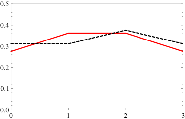
(a) $d=3$

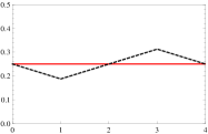
(b) $d=4$

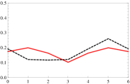
(c) $d=6$

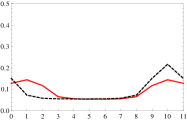
(d) $d=11$

Figure 1: Limiting probability distributions for Hadamard quantum walks with one-step memory on cycle with $d=3,4,6$ and $11$ nodes for the initial states given by Eq. (21) (solid red line) and $|\phi_{1}\rangle=(1,0,0,0)^{T}$ (dashed black line). For each $d$ the results are plotted in range $[0,\dots,d]$ to illustrate the periodicity of the limiting distribution. Nodes are numbered starting from 0.

One can observe that the convergence of $\bar{p}(n)$ depends only on the behavior of the term

$$f(k,j,m,l)\equiv\lim_{t\rightarrow\infty}\frac{1}{t}\sum_{s=0}^{t-1}\left[\lambda_{j}^{\star}(k)\lambda_{l}(m)\right]^{s}.$$ (32)

The value of this functions depends on the product of eigenvalues as

$$f(k,j,m,l)=\left\{\begin{array}[]{cr}1&\ \mathrm{if}\ \lambda_{j}^{\star}(k)\lambda_{l}(m)=1\\ 0&\ \mathrm{otherwise}\hfill\end{array}\right..$$ (33)

Unfortunately, any further simplifications of Eqs. (29) and 30) were not possible. In particular, this simplification requires a closed form for the product of eigenvalues, $\lambda_{j}^{\star}(k)\lambda_{l}(m)$. However, definition in Eq. (33) can be easily calculated using the standard computer algebra systems, and thus allows for the evaluation of Eq. (30).

The examples of time-averaged limiting distribution for the discussed model calculated using Eq. (30) are presented in Fig. 1 and Fig. 2

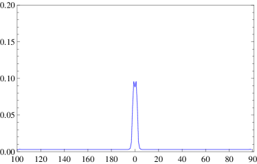
(a) $d=200$, $|\phi_{0}\rangle$

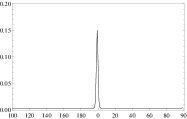
(b) $d=200$, $|\phi_{1}\rangle$

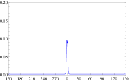
(c) $d=300$, $|\phi_{0}\rangle$

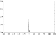
(d) $d=300$, $|\phi_{1}\rangle$

Figure 2: Limiting probability distributions for Hadamard quantum walks with one-step memory on cycle with $d=200$ (2(a) and 2(b)) and $d=300$ (2(c) and 2(d)) nodes. Result were obtained for initial state $|\phi_{0}\rangle$ – 2(a) and 2(c) – and initial state $|\phi_{1}\rangle$ – 2(b) and 2(d). For the large number of nodes the only significant contributions stem from the nodes close to the starting node.

In order to illustrate the influence of the initial state on the resulting distribution, two initial states were used to obtain these plots. In the case of the input state given by Eq. (21), the memory register is in the superposition, and the resulting time-averaged probability distribution is symmetric with respect to the starting position. On the other hand, if the memory register is set to $|0\rangle$ in the initial state, the resulting time-averaged probability distribution does not have this property.

Comparison of the limiting probability distribution for larger numbers of nodes is presented in Fig. 2. One can see that in these case the only significant contributions stem from the nodes close to the starting node.

The important difference in comparison with the memoryless quantum walk on cycle is that the time averaged limiting distribution depends on the initial state of the coin and the memory registers, but not on the parity of the number of nodes $d$ travaglione02implementing ; bednarska03walks . The dependency is expressed in the $\alpha_{j}(k)$ coefficients, which are defined in Eq. (26).

IV Summary

We have introduced a model of quantum walk with memory on cycle and studied its basic properties. We have calculated the probability of finding the particle at each position after given number of steps and we have provided a formula for the time-averaged limiting probability distribution for the discussed model. We have also pointed out the most important differences between quantum walks on cycles with and without memory. The most important difference is that the symmetry of the time-averaged limiting probability distribution is independent of the parity of the number of nodes. However, this distribution is heavily influenced by the initial state of the memory register.

References

[1]
D. Aharonov, A. Ambainis, J. Kempe, and U. Vazirani.
Quantum walks on graphs.
In Proceedings of the 30th Annual ACM Symposium on Theory of
Computation, pages 50–59. ACM Press, 2001.
[2]
A. Ambainis.
Quantum walks and their algorithmic applications.
Int. J. Quant. Inf., 1:507–518, 2003.
[3]
A. Ambainis.
Quantum walk algorithm for element distinctness.
SIAM Journal on Computing, 37:210–239, 2007.
[4]
M. Bednarska, A. Grudka, P. Kurzyński, T. Łuczak, and A. Wójcik.
Quantum walks on cycles.
Phys. Lett. A, 317(1-2):21–25, 2003.
[5]
T.A. Brun, H.A. Carteret, and A. Ambainis.
Quantum walks driven by many coins.
Phys. Rev. A, 67:052317, 2003.
[6]
H. Buhrman and R. Špalek.
Quantum verification of matrix products.
In Proceedings of the seventeenth annual ACM-SIAM symposium on
Discrete algorithm, pages 880–889. ACM, 2006.
[7]
A.M. Childs and J.M. Eisenberg.
Quantum algorithms for subset finding.
Quantum. Inf. Comput., 5:593, 2005.
[8]
A.M. Childs and J. Goldstone.
Spatial search by quantum walk.
Phys. Rev. A, 70(2):022314.1, 2004.
[9]
A.P. Flitney, D. Abbott, and N.F. Johnson.
Quantum random walks with history dependence.
J. Phys. A, 37:7581–7591, 2004.
[10]
G. Grimmett, S. Janson, and P.F. Scudo.
Weak limits for quantum random walks.
Phys. Rev. E, 69(2):026119, Feb 2004.
[11]
N. Konno and T. Machida.
Limit theorems for quantum walks with memory.
Quant. Inf. Comp., 10(11&12):1004–1017, 2010.
[12]
F. Magniez, M. Santha, and M. Szegedy.
Quantum algorithms for the triangle problem.
In Proceedings of the sixteenth annual ACM-SIAM symposium on
Discrete algorithms, pages 1109–1117. Society for Industrial and Applied
Mathematics, 2005.
[13]
M. Mc Gettrick.
One dimensional quantum walks with memory.
Quant. Inf. Comp., 10(5&6):0509–0524, 2010.
[14]
A. Nayak and A. Vishwanath.
Quantum walk on the line.
arXiv:quant-ph/0010117, 2000.
[15]
D. Reitzner, D. Nagaj, and V. Bužek.