The Ionized Absorber and Nuclear Environment of IRAS 13349+2438: Multi-wavelength insights from coordinated Chandra HETGS, HST STIS, HET, and Spitzer IRS

Abstract

We present results from a multiwavelength IR–to–X-ray campaign of the infrared bright (but highly optical-UV extincted) QSO IRAS 13349+2438 obtained with the Chandra High Energy Transmission Grating Spectrometer (HETGS), the Hubble Space Telescope Space Telescope Imaging Spectrograph (STIS), the Hobby-Eberly Telescope (HET) 8-meter, and the Spitzer Infrared Spectrometer (IRS). Based on HET optical spectra of $[$O iii$]$, we refine the redshift of IRAS 13349 to be $z=0.10853$. The weakness of the $[$O iii$]$ in combination with strong Fe  ii in the HET spectra reveal extreme Eigenvector-1 characteristics in IRAS 13349, but the 2468 ${\rm\thinspace km}{\rm\thinspace s}^{-1}\,$width of the H$\beta$ line argues against a narrow-line Seyfert 1 classification; on average, IR, optical and UV spectra show IRAS 13349 to be a typical QSO. Independent estimates based on the H$\beta$ line width and fits to the IRAS 13349 SED both give a black hole mass of $M_{\rm BH}=10^{9}~{}M_{\odot}$. The heavily reddened STIS UV spectra reveal for the first time blue-shifted absorption from Ly $\alpha$, N v and C iv, with components at systemic velocities of $-950~{}\hbox{${\rm\thinspace km}{\rm\thinspace s}^{-1}\,$}$ and $-75~{}\hbox{${\rm\thinspace km}{\rm\thinspace s}^{-1}\,$}$. The higher velocity UV lines are coincident with the lower-ionisation ($\xi\sim 1.6$) WA-1 warm absorber lines seen in the X-rays with the HETGS. In addition, a $\xi\sim 3.4$ WA-2 is also required by the data, while a $\xi\sim 3$ WA-3 is predicted by theory, and seen at less significance; all detected X-ray absorption lines are blueshifted by $\sim 700-900$${\rm\thinspace km}{\rm\thinspace s}^{-1}\,$. Theoretical models comparing different ionising SEDs reveal that including the UV (i.e., the accretion disc) as part of the ionising continuum has strong implications for the conclusions one would draw about the thermodynamic stability of the warm absorber. Specific to IRAS 13349, we find that an X-ray-UV ionising SED favors a continuous distribution of ionisation states in a smooth flow (this paper), versus discrete clouds in pressure equilibrium (previous work by other authors). Direct detections of dust are seen in both the IR and X-rays. We see weak PAH emission at 7.7 $\mu{\rm m}\;$and 11.3 $\mu{\rm m}\;$which may also be blended with forsterite, and 10 $\mu{\rm m}\;$and 18 $\mu{\rm m}\;$silicate emission, as well as an Fe L edge at 700 eV indicative of iron-base dust with a dust-to-gas ratio $>90$%. We develop a geometrical model in which we view the nuclear regions of the QSO along a line of sight that passes through the upper atmosphere of an obscuring torus. This sight line is largely transparent in X-rays since the gas is ionised, but it is completely obscured by dust that blocks a direct view of the UV/optical emission region. In the context of our model, 20% of the intrinsic UV/optical continuum is scattered into our sight line by the far wall of an obscuring torus. An additional 2.4% of the direct light, which likely dominates the UV emission, is Thomson-scattered into our line-of-sight by another off-plane component of highly ionized gas.

1 Introduction

IRAS 13349+2438, hereafter “IRAS 13349”, ($z=0.10764$ – Kim et al. 1995; updated here to $z=0.108530$ based on the 3$\times$ higher resolution HET spectra reported in this paper) is a prototype infrared-luminous quasar with a bolometric luminosity of $\mathrel{\hbox to0.0pt{\lower 3.0pt\hbox{$\sim$}\hss}\raise 2.0pt\hbox{$>$}}2\times 10^{46}$ erg s^-1 (Beichman et al., 1986). Images of the host galaxy and nearby environment show the galaxy to be spiral-like, with a possible companion at $\sim$ 5^′′ along the minor axis (e.g., Hutchings & McClure 1990). Evidence for tidal structure suggests that the object may have interacted with the companion, and this could supply gas and dust to the nucleus, fueling quasar activity and enhancing nuclear obscuration and scattering. Indeed, IRAS 13349 has a broad-emission line optical spectrum that becomes heavily reddened at shorter wavelengths, and exhibits high optical continuum and emission-line polarisation (Wills et al., 1992, hereafter W92). The observed polarisation rises strongly toward shorter wavelengths, but the optical polarised flux spectrum is indistinguishable from a typical, unreddened quasar (Hines et al. 2001). These polarisation properties indicate that observers see the quasar’s nucleus via both a direct, but attenuated, light path and a scattered light path (W92; Hines et al., 2001). In addition to its high luminosity and spectral variability, IRAS 13349 also exhibits strong Eigenvector-1 characteristics (strong optical Fe ii emission and weak $[$O iii$]$ relative to $\rm H\beta$; Boroson & Green 1992). It is typically identified to be radio-quiet, although weak 4.87 mJy radio emission has been reported at 6 GHz by Laurent-Muehleisen et al. (1997).

The observed high X-ray flux and large-amplitude X-ray variability indicate that a large fraction of the X-ray emission is seen via a direct, rather than a scattered, path. As such, IRAS 13349 has been the subject of a number of X-ray studies that have helped to clarify the physical processes in the inner regions of the quasar nucleus. Using XMM-Newton EPIC data, Longinotti et al. (2003) made a detailed analysis of the IRAS 13349 ionised reflection spectrum and relativistic Fe emission line. At lower energies, X-ray studies based on the ROSAT  PSPC (Brandt et al., 1996) and ASCA (Brandt et al., 1997), combined with optical/near-infrared extinction estimates argue for obscuration by dusty, ionised gas. Studies with modern day high spectral resolution instruments on board XMM-Newton (Sako et al., 2001), and Chandra (Holczer et al. 2007; Behar 2009; also this paper) reveal additional complexity in the absorbers (most notable an unresolved transition array of 2p-3d inner-shell absorption by iron M-shell ions, dubbed the UTA by its discoverers, Sako et al.), and allow direct measurements of the dust composition (this paper) in the host galaxy.

In this paper, we present a comprehensive analysis of the absorber properties of this quasar, based on our high spectral resolution, multi-wavelength campaign, involving X-ray (with the Chandra High Energy Transmission Grating Spectrometer; HETGS), ultraviolet (with HST STIS-MAMA), optical (HET: Hobby-Eberly Telescope 8-m), and infrared (Spitzer IRS) observations. The Chandra and HST observations are simultaneous, HET near simultaneous, and Spitzer IRS taken 1.25 years later as part of the GTO program of G. Rieke. These high-quality data allow us to address, in detail for a specific luminous system, several issues of broader importance in active-galaxy absorption studies. These include the apparent presence of dust in some ionized absorbers and its implications for interpreting observations; the relation of ionized absorbers to other nuclear components, including accretion disks, tori, and scattering material; the relation of the spectral energy distribution (SED) to the structure of ionized absorbers; and the potential for feedback into host galaxies by outflowing nuclear winds.

The paper is organised as follows. In Section 2, the multi-wavelength data are presented, to be followed by a plasma diagnostic approach to the line analysis in Section 3. In Section 4 we combine our multi-wavelength data with additional ISO and IRAS archived observations to produce an observed SED that is used to determine a theoretically motivated ionising spectrum affecting the warm absorber properties; this then is used to generate ion populations with xstar for our spectral fitting. This will set the stage for Section 5 considerations on the warm absorber behaviour as established by thermodynamic stability arguments (Section 5.1), and complex line-of-sight geometry through dust (Section 5.2). We adopt $H_{0}=73$ km s^-1 Mpc^-1, $\Omega_{\rm M}=0.25$, and $\Omega_{\Lambda}=0.75$ throughout this paper.

2 Observations & Data Reduction

As part of a multi-wavelength campaign to better understand the global physical processes, absorber kinematics, and geometry of IRAS 13349, we observed this nearby quasar using spectrographs on Chandra (X-ray), the Hubble Space Telescope (ultraviolet), the Hobby-Eberly Telescope 8-meter (optical), and the Spitzer Space Telescope (infrared; Werner et al. 2004). Observations performed with Chandra , HST and HET were nearly simultaneous and of comparable spectral resolution ($R\sim 1000$), while “high” (R $\sim 600$) and low-resolution (R $\sim 70-120$) IR spectra from Spitzer were obtained $\sim 1.25$ years later as part of the GTO program of George Rieke.

Table 1: Chandra Observations

Date	Start Time	End Time	Useable Time
	(GMT)	(GMT)	(ks)
2004-02-22	06:42:06	…
2004-02-23	…	12:15:15	160
2004-02-24	13:56:00	…
2004-02-26	…	11:16:41	135

2.1 X-ray Observations with the Chandra HETGS

IRAS 13349 was observed with the Chandra HETGS (High Energy Transmission Grating Spectrometer: Canizares et al. 2005; Weisskopf et al. 2002) over several days in 2004 February for a total of $\sim$ 295 ks of usable data as summarised in Table 1. Plus and minus first order ($\pm 1$) spectra were extracted using the latest ciao release (ciao 4.3 with caldb 4.4.3), starting with the L1 (raw unfiltered event) files, which we reprocess to remove hot pixels and afterglow events. In order to maximise signal-to-noise (S/N), we combine plus and minus 1st orders for both the HEG and MEG. The resolving power of the HETGS is $\rm E/\Delta E=1000$. We focus on the $\sim 1.5-26$ Å  (0.45$-$8 keV) spectral region in this paper, with particular emphasis on the soft (0.5-5 keV; 2.5-26Å) band of the warm absorber. Analysis of the Chandra line spectra was done within the isis analysis package.

2.2 Simultaneous UV Observations with the Hubble Space Telescope STIS MAMA

Simultaneous HST  (Hubble Space Telescope) UV spectra were obtained using the Space Telescope Imaging Spectrograph (STIS) (Woodgate et al., 1998). The faintness of IRAS 13349 in the UV made the STIS echelle mode an impractical choice, so we observed IRAS 13349 through the $52\times 0.5~{}$^′′slit with the UV MAMA detectors and the low resolution UV gratings (R$\sim 1000$) G140L and G230L in a 4-orbit visit on 2004 Feb 22 starting at GMT 08:09:48. Table 2 summarises the STIS observations.

Table 2: STIS Observations

Data Set Name	Grating	Date	Start Time	Exposure Time
			(GMT)	(s)
o8wp01010	G140L	2004-02-22	08:09:48	2000
o8wp01020	G140L	2004-02-22	09:31:42	2630
o8wp01030	G140L	2004-02-22	11:08:22	2630
o8wp01040	G230L	2004-02-22	12:44:03	2630

Three exposures with G140L totaling 7260 s and one exposure with G230L totaling 2630 s gave a spectrum covering the 1150–3180Å  spectral range. The G140L spectrum has a resolving power that varies with wavelength of 960–1440 over its full spectral range; for G230L the resolving power is slightly lower, 530–1040.

We used the extracted one-dimensional spectra as produced by the STScI pipeline for our analysis. Our data required only a slight zero-point adjustment ($<1$ pixel, corresponding to $<100$ ${\rm\thinspace km}{\rm\thinspace s}^{-1}\,$in each exposure) to the wavelength scale which we determined using the Galactic absorption lines in our spectra. Observations of Galactic H i along this sight-line by Murphy et al. (1996) show an optically thin column density of $1.07\times 10^{20}~{}\rm cm^{-2}$ at a mean heliocentric velocity of $-19~{}\rm km~{}s^{-1}$. In the region of wavelength overlap between the G140L and the G230L spectra, the flux levels agree to $<$0.7%. We have made no adjustments to either flux scale, given that an absolute accuracy of better than 4% is expected (Bostroem, 2010).

2.3 Near Simultaneous Optical Observations with the Hobby-Eberly 8-meter

Since IRAS 13349 shows large-amplitude variability at X-ray wavelengths, we also obtained a near-simultaneous spectrum of it with the 8-meter Hobby-Eberly Telescope (HET; Ramsey et al. 1998) to constrain its optical properties during the Chandra  and HST  observations. (We note that while the HET is officially designated a 9.2-meter telescope, we conservatively refer to it here as an 8-meter class given that this is the average equivalent aperture for a typical observation – see Schneider et al. 2000.) HET observations were obtained on 2004 Feb 26 with the Marcario Low-Resolution Spectrograph (Hill et al., 1998a, b). The observations were taken with a 600 line mm^-1 grating, a slit width of $1^{\prime\prime}$, and a GG385 blocking filter, resulting in a resolving power of 1300 over the observed wavelength range 4300–7300 Å. The total exposure time of 1283.5 s was split among four sub-exposures. For flux calibration, we observed the white-dwarf standard Feige 34 during the middle of the night, two hours prior to our observation of IRAS 13349. Exposures on a Cd-Ne arc lamp were used to determine the wavelength scale, with zero points adjusted using the night-sky lines in our spectra. Final flux-calibrated spectra were extracted with the standard IRAF reduction codes for single-slit data.

2.4 Infrared observations with the Spitzer IRS

Low-resolution ($R=70-120$) and high-resolution ($R\sim 600$) infrared spectra were obtained as part of the GTO program of Rieke (PID: 61) on 2005 June 7 with the Infrared Spectrograph (IRS, Houck et al., 2004) on the Spitzer Space Telescope (Werner et al., 2004) using the standard staring mode. In each spectroscopic module, the source was observed at two nodding positions, and exposure times were set to $2\times 5\times 14$ s in SL (Short-Low) and LL (Long-Low), as well as $2\times 5\times 120$ s and $2\times 10\times 60$ s in SH (Short-High) and LH (Low-High), respectively.

The low-resolution spectral data (LRS) were reduced, from the basic calibration data (BCD) files, following the standard procedure given in the IRS Data Handbook. The basic steps were bad-pixel correction with irsclean v2.1, background subtraction using the off-source slit, as well as optimal extraction and wavelength/flux calibration with the Spectroscopic Modeling Analysis and Reduction Tool suite (SMART v8.2.1; Higdon et al. 2004), for each nodding position. Spectra were then nod-averaged to improve the signal-to-noise ratio (S/N).

The flux calibration appeared consistent between the different modules, with differences less than 5%, and this allowed us to combine all the spectra to cover the 5.2$-$35 $\mu$m spectral range (4.7$-$32 $\mu$m rest frame). Nevertheless, the continuum at 25 $\mu$m showed a multiplicative offset from the IRAS 13349 photometric flux at 25 $\mu$m  obtained from the IRAS Point Source Catalog (hereafter, IRAS-PSC). Unfortunately, there is no associated MIPS 24 $\mu$m photometry during the epoch of the Spitzer IRS observation, so we cannot rule out the possibility that the object has varied in this energy band. However, given that IRAS 13349 is radio quiet, and that the shape of the SED suggests that the mid-IR is produced by thermal emission from dust heated by the central engine, we assume that the mid-IR has not varied. We therefore scaled the entire spectrum by a factor of 1.077 to match the (un-color-corrected) IRAS-FSC flux density measurement of 0.84$\pm$0.06 Jy at 25 $\mu$m.

Table 3: Ionic columns densities based on fits to Chandra observed lines from the full transition series

Ion	a$\;\;n_{\rm detected}$	b$\;\;\rm v_{blue}$	c$\;\;\rm b$	d$\;\;\rm\,log\,N_{j}$	e$\;\;\rm b$	f$\;\;\rm\,log\,N_{j}$	g$\;\;\rm\,N_{H}$
		($\rm km\,s^{-1}$)	($\rm km\,s^{-1}$)	($\rm cm^{-2}$)	($\rm km\,s^{-1}$)	($\rm cm^{-2}$)	($\rm 10^{21}\,cm^{-2}$)
O vii	2 - $\infty$	$-748^{+103}_{-126}$	$137^{+39}_{-74}$	$18.1\pm 0.5$	100	$17.8\pm 0.5$	$1.48$
O viii	2 - $\infty$	$-595^{+99}_{-107}$	$288^{+89}_{-92}$	$17.8^{+0.2}_{-0.3}$	100	$17.6^{+0.4}_{-0.5}$	$0.94$
Ne ix	2 - $\infty$	$-788^{+131}_{-168}$	$519^{+117}_{-133}$	$17.3^{+0.1}_{-0.2}$	100	$17.7^{+0.7}_{-0.5}$	$8.15$
Ne x	2 - 6	$-833^{+354}_{-160}$	$284^{+164}_{-139}$	$17.3^{+0.3}_{-0.4}$	100	$17.4^{+0.4}_{-0.6}$	$4.08$
Mg xi	2 - 4	$-578^{+212}_{-145}$	$150^{+79}_{-140}$	$17.4^{+3.8}_{-0.4}$	100	$17.4^{+0.4}_{-0.5}$	$13.0$
Mg xii	2 - 4	$-675^{+157}_{-123}$	$133^{+87}_{-78}$	$17.4^{+0.4}_{-0.7}$	100	$17.4^{+0.4}_{-0.7}$	$13.0$
Si xiii	2 - 3	$-537^{+156}_{-134}$	$48^{+447}_{-38}$	${}^{+}_{-}$	100	$17.6^{+1.0}_{-1.1}$	$22$

See corresponding curve-of-growth plots in Figure 1.
^a Transitions in series which contribute to the best fit $N_{\rm j}$; $\infty$ correspond to series limit.
^b Outflowing velocity measured against the laboratory wavelengths tabulated by Verner et al. (1996)
^c Turbulent velocity width ($\rm km\,s^{-1}$) as determined from the series fit. See §3.1 for discussion on caveats.
^d Corresponding ionic column density ($\rm cm^{-2}$).
^e Turbulent velocity width frozen at 100 ${\rm\thinspace km}{\rm\thinspace s}^{-1}\,$. See §3.1 for discussion on reasoning behind this.
^f Corresponding ionic column density ($\rm cm^{-2}$).
^g Corresponding equivalent Hydrogen column assuming the solar abundance values given by Wilms et al. (2000). Note however that the numbers assume an ionization fraction for all ions to be 50%; as such, quoted numbers are only rough guides, and not to be directly taken at face value.

We reduce the high-resolution spectral data (HRS) in much the same way as previously described for the LRS, with the exception that full-aperture instead of optimal extraction is employed, the distinction being that pixels along the dispersion axis have equal (full-aperture) versus varied (optimal) weighting. Moreover, we could not remove background by on-source/off-source subtraction, due to the lack of off-source HRS background files in the IRS archives associated with the epoch of this observation. Therefore, we extract SL1, LL2, and LL1 backgrounds from the low-resolution data and fit with first-order polynomials. We then use these fits to remove the background contribution from the high-resolution spectra, giving a good match between the SH and LH continuum flux density level. Finally, the overall high-resolution spectrum is scaled by 1.077 to match the continuum flux density level at 25 $\mu$m to the IRAS 13349 IRAS-PSC photometric flux density at the same wavelength.

                 

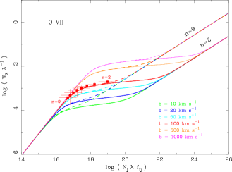
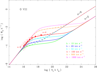
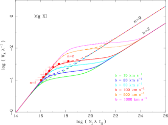
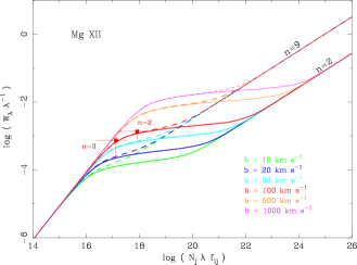
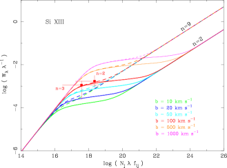
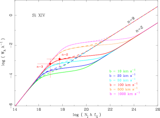
Figure 1: Curve-of-growth calculations representing $n=2$ and $n=9$ transitions for H-like 1s-1s$n$p and He-like $1s^{2}$–$1snp$ transitions for different values of the turbulent velocity width $b$. Plotted data point represent $N_{\rm j}\;$values measured based on a simultaneous fit to all the lines detected for a given H- or He-like resonance series, assuming $b=100$${\rm\thinspace km}{\rm\thinspace s}^{-1}\,$. E.g. plotted points represent a fit (with oscillator strengths locked in the appropriate ratios) to the detected $n=2$ to $n=9$ lines of He-like $1s^{2}$–$1snp$ O vii whereas a fit to the H-like Mg xii only includes a fit to the $n=2$ and $n=3$ lines. (See Section 3.1 and Table 3 for details.) The purpose of the exercise is to demonstrate the importance of the higher order lines for establishing true $N_{\rm j}\;$derivations, where fits to single lines (especially the $n=2$ $\alpha$-transition which may lie on the saturated part of the COG) may give an $N_{\rm j}\;$with possible values that span up to two orders of magnitude.

3 Data Analysis and Line Detections

The intent of this paper is to provide the highest spectral resolution multi-wavelength characterisation of the IRAS 13349 spectrum to date, as a step toward a more detailed understanding of the structure of this quasar and its host galaxy. For this paper, we employ both a plasma-diagnostic approach to the analysis (this section), as well as photoionization modeling with xstar (Kallman & Bautista, 2001) for a global analysis (§4) of the spectra based on the observed multi-wavelength spectral energy distribution (SED).

3.1 The X-ray Chandra HETGS spectrum

Figure 2: Velocity spectra obtained by co-adding the 5 strongest resonance lines for H and He like ions of nitrogen, oxygen, neon, magnesium, aluminium, silicon, and sulfur. For N, O, Ne, and Mg ions, MEG grating spectra are co-added, whereas HEG data are used for Al, Si, and S. We bin at 200 $\rm{km\,s^{-1}}$ in velocity; S is binned at 400 $\rm{km\,s^{-1}}$. – Velocity bins are chosen to reflect the approximate FWHM resolution of the HETGS at the energies where these ions are found. To guide the eye, vertical lines denote velocities corresponding to 0, -1000 and -2000 $\rm{km\,s^{-1}}$. Multiple absorption components appear strongest for O, Ne, Mg, and Si. The errors are Poisson and each bin is independent despite appearances to the contrary.

We begin initially with a plasma diagnostic approach to the line fits. To search for individual absorption and emission lines, HETGS spectra were binned by two, corresponding to half the spectral resolution, respectively 0.006Å  and 0.012Å FWHM, for the HEG and MEG. For these fits, we use a fifth order polynomial to fit local continua, rather than a phenomenological broad-band continuum. Such an approach allows us to remove the broader fluctuations, thereby maximising our ability to measure the narrow lines without assumptions about details of the continuum, which can be complex. Using this analysis procedure, we find the X-ray spectrum to be dominated by an ionised absorber giving rise to prominent H- and He-like absorption lines of oxygen, neon, magnesium, and silicon, as well as absorption lines from a variety of iron ions, at a bulk outflow velocity in the range $-900~{}\hbox{${\rm\thinspace km}{\rm\thinspace s}^{-1}\,$}\mathrel{\hbox to0.0pt{\lower 3.0pt\hbox{$\sim$}\hss}\raise 2.0pt\hbox{$<$}}v_{\rm x-ray}\mathrel{\hbox to0.0pt{\lower 3.0pt\hbox{$\sim$}\hss}\raise 2.0pt\hbox{$<$}}-500~{}\hbox{${\rm\thinspace km}{\rm\thinspace s}^{-1}\,$}$.

Since a comprehensive photoionization treatment of the IRAS 13349 absorber as tied to its SED and theory considerations, is explored in detail in Section 4, we concentrate here primarily on the key H- and He-like ions as a model-independent way of accessing the QSO hot plasma conditions for comparison with later analysis. For many of these key ions, high order transitions, corresponding to a high column density warm absorber is detected (see Table 3). For these key ions, we derive the individual ionic column densities ($N_{\rm j}\;$) based on a fit to the entire detected resonance series of lines from $n$=2–$xx$, where $xx$ is the highest transition detected; e.g. H-like $1s-np$ Mg xii and He-like $1s^{2}-1snp\,$Mg xi are detected to $n=4$ so that our fits to those series are to the Ly/He-($\alpha,\beta,\gamma,\delta)$ lines with their oscillator strengths locked to their tabulated value as found e.g. in Verner et al. (1996). The individual lines in the series are fit using Voigt profiles, although the derived $N_{\rm j}\;$is based on a simultaneous fit to all the detected lines in the series. In this way, we ensure the best possible determination of $N_{\rm j}\;$(Table 3) by reducing the possibility for false estimates resulting from saturated or contaminated lines. (Both saturated and contaminated lines can falsely indicate a line width and strength which is broader and has higher flux than what it truly is for the ion, thereby resulting in lower estimates for any given ionic column.) We note however, that despite these precautions, the spectral resolution of the Chandra HETGS, while the best available to date, is still not sufficient for probing at the level of measuring the $10-20$ ${\rm\thinspace km}{\rm\thinspace s}^{-1}\,$thermal widths of these ions. As such, $N_{\rm j}\;$estimates may only be lower limits. For thoroughness, we adopt a value for the turbulent velocity width $b=100$ ${\rm\thinspace km}{\rm\thinspace s}^{-1}\,$to approximate the Chandra HETGS spectral resolving capabilities, for deriving the ionic columns noted in Table 3; we also detail the associated ionic columns based on fits where $b$ is allowed as a free parameter. For Ne ix (and to a lesser extent Ne x), Fe contaminates many of the stronger lines in the series, resulting in a larger measured $b$, and hence smaller $N_{\rm j}\;$.

It is also clear that the measured value of $N_{\rm j}\;$strongly depends on $b$ as best illustrated by the curve-of-growth (COG) plots in Figure 1. Here, we plot COG calculations (which include the damping parameter as presented e.g. in Spitzer 1978) for different values of the turbulent width, which range from $b=10-20$ ${\rm\thinspace km}{\rm\thinspace s}^{-1}\,$($\approx$ the thermal width value of the ion), to $b=100$ ${\rm\thinspace km}{\rm\thinspace s}^{-1}\,$(maximal resolving power of the HETGS), to $b=1000$ ${\rm\thinspace km}{\rm\thinspace s}^{-1}\,$(the approximate value derived by Sako et al. 2001 in their analysis of the XMM RGS spectrum). For each ion, two sets of curves corresponding to the $1\rightarrow 2$ (Ly / He $\alpha$) and $1\rightarrow 9$ (representing the series limit) transitions are shown. Over plotted as individual points on the curves are the values for the different transitions which are detected in our data, and which contribute in the series fitting of the $N_{\rm j}\;$values listed in Table 3, for fixed values of $b=100$ ${\rm\thinspace km}{\rm\thinspace s}^{-1}\,$. It is clear that for any given ion, a detection of the higher transition series better aids in the determination of $N_{\rm j}\;$. This is well illustrated in a comparison of the H- and He-like oxygen series which are detected to the series limit versus the H- and He-like silicon series, where only the $\alpha$ ($1\rightarrow 2$) and $\beta$ ($1\rightarrow 3$) transitions contribute significantly to the fitting. H- and He-like Ne have been excluded from the figure due to significant contamination from Fe. For the other ions in the figures, contamination to the line series comes from other velocity components of the same ions – e.g. for He-like O vii , components 1, 2, 3 of the warm absorbers discussed in §4.3 all contribute to the line series at different velocities.

To assess further the presence of multiple velocity components, we generate velocity spectra based on the 5 strongest resonance transitions for the most prominent X-ray ions, namely H- and He-like ions of nitrogen, oxygen, neon, magnesium, aluminium, silicon and sulphur. (note that not all these are necessarily detected.) For each individual absorption line, a velocity grid from -4000 to 4000 ${\rm\thinspace km}{\rm\thinspace s}^{-1}\,$is generated centered around the rest wavelength of the particular line, i.e. zero velocity corresponds to the rest wavelength of the line of choice. The HETGS spectra of counts vs wavelength (initially binned by 4) is remapped (through interpolation) to convert to the velocity space. Standard error propagation rules are invoked and the remapping retains the Gaussian nature of the errors (i.e. $\sqrt{(}\rm{counts})$). The velocity spectra of the five strongest resonance lines are then combined (errors are added in quadrature) to represent the velocity spectrum of the concerned ion. Figure 2 shows the velocity profiles derived in the aforementioned way. The velocity is binned at 200 $\rm{km\,s^{-1}}$ except for the bottom most panel (i.e. for sulphur) where the binning is at 400 $\rm{km\,s^{-1}}$. At wavelengths corresponding to the sulphur lines, which have been considered, the velocity resolution for HEG is $>400\rm{km\,s^{-1}}$. To achieve the best results we have used MEG spectra for N, O, Ne and Mg while resorting to HEG for Al, Si and S having higher energy transitions. The figure clearly shows detection of absorption for O, Ne, Mg, Al and Si. The N ions show a hint of absorption, whereas no absorption is detected for S ions. We have also looked for absorption in carbon, argon and calcium with no significant detection. For most of the ions the velocity profiles do not have a symmetric Gaussian distribution indicating the presence of more than one velocity component. We will return to a discussion of the X-ray lines in §4.3.

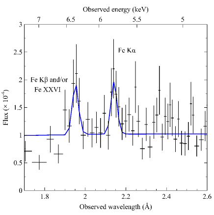
Figure 3: The Chandra HETGS spectra at $>6$ keV reveal two prominent emission lines, one due to Fe i K$\alpha$ at rest energy 6.4 keV and another similarly strong line at $\sim 7$ keV that may be identified with H-like Fe xxvi or Fe i K$\beta$ blended with a broadened component of the Fe i K$\alpha$ line.

Figure 4: HST/STIS low-resolution spectrum of IRAS13349+2438 in observed wavelengths. Prominent emission lines are marked.

3.1.1 Ionized and neutral emission lines

By far the strongest detected narrow X-ray emission line is the Fe i K$\alpha$ fluorescent line at $\sim 6.4$ keV (rest) with flux $F_{\rm{K}\alpha}\sim 4\times 10^{-6}$ ${\rm\thinspace ph}{\rm\thinspace cm}^{-2}{\rm\thinspace s}^{-1}\,$(Fig. 3; also Fig. 13). Another strong line of approximately equal strength appears at rest energy $\sim 7$ keV (Table 8). This energy is best matched to Fe i K$\beta$ but this gives an unphysical K$\alpha$:K$\beta\sim 1$, when the ratio should be $\sim 10$. However, given the claim by Longinotti et al. (2003) based on XMM data for a complex iron line that has a narrow component on top of a relativistically broadened line, the most likely explanation for the measured similarities in the K$\alpha$ and K$\beta$ line fluxes here is that what we have measured in the Chandra data is only a small portion of the broadened line. Since a discussion of relativistic effects is not the goal of this paper, we will leave it at a reporting of the line measurements at high spectral resolution. An alternative possibility, especially given the line strength is that the emission is in fact due to Fe xxvi K$\alpha$ at 6.96 keV. We have also checked the $\sim$ 6–8 keV spectral region for emission from other ions (e.g. 6.7 keV Fe xxv K$\alpha$, 7.5 keV Ni i K$\alpha$, and 8.26 keV Ni i K$\alpha$), but find no significant detections.

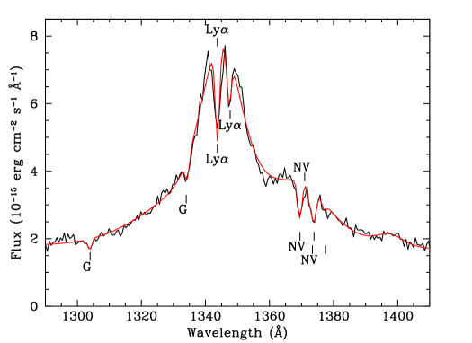
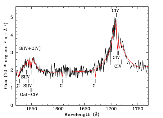
Figure 5: Detail of the STIS G140L spectrum of IRAS13349+2438, in observed wavelengths, in the Ly$\alpha$ region (top panel) and the C iv region (bottom panel). The black curves are the observed data; the red curves are the best fit to the spectrum. Emission features are labeled above the spectra, and absorption components are marked below. The “G” labels denote foreground Galactic interstellar absorption lines.

3.2 The UV HST STIS-MAMA Spectra

To measure the UV fluxes, widths, and redshifts of the emission and absorption lines, we used the IRAF task specfit (Kriss, 1994). As discussed in §5.2, the full continuum is a complex mix of direct light from the active nucleus that is heavily reddened combined with light scattered from dust, and perhaps free electrons also, that also suffers some extinction. We were unable to arrive at a model that fully matched the observed shape of the full continuum, so, to characterise the emission and absorption lines, we used an empirical approach that simply fit a power law that was locally optimised around each emission-line blend. Nearly all emission lines required both a broad ($\sim 2500\hbox{${\rm\thinspace km}{\rm\thinspace s}^{-1}\,$}$ in width) and a very broad ($\mathrel{\hbox to0.0pt{\lower 3.0pt\hbox{$\sim$}\hss}\raise 2.0pt\hbox{$>$}}7500\hbox{${\rm\thinspace km}{\rm\thinspace s}^{-1}\,$}$) component to obtain an adequate fit. Table 4 gives the fluxes, velocities, and full-width at half-maximum (FWHM) for the fitted emission lines. Velocities are relative to the systemic redshift of $z=0.10853$, based on the observed redshift of the [O iii] $\lambda 5007$ emission line in our HET spectrum (see §3.3 for details). The tabulated line widths are corrected for instrumental resolution by subtracting the resolution in quadrature from the measured widths. Wavelengths $<1720$ Å have the resolution of the STIS G140L grating as given in the STIS Instrument Handbook, ranging from 0.93 Å at 1350 Å to 0.81 Å at 1700 Å. Longer wavelengths have the resolution of the G230L grating, which is 3.40 Å.

Figure 6: The HET spectrum of IRAS 13349, in observed wavelengths, shows a typical quasar spectrum dominated by broad Balmer emission lines and $[$O iii$]$, with the exception of particularly strong Fe ii. The lone absorption can be attributed to atmospheric Franhofer B-band which we have not corrected for, since it has no effect on the conclusions derived from our spectrum.

Table 4: UV & Optical Emission Lines in IRAS13349+2438

Line	$\rm\lambda_{0}$a	Fluxb	Velocityc	FWHM
	(Å)		$\rm(km~{}s^{-1})$	$\rm(km~{}s^{-1})$
Hubble Space Telescope UV Spectrum (Figure 5)
Ly $\alpha$	1215.67	$\phantom{0}5.3\pm 0.1$	$-710\pm 368$	$3026\pm 150$
Ly $\alpha$	1215.67	$10.2\pm 0.1$	$-710\pm 368$	$10018\pm 140$
N v	1240.15	$\phantom{0}1.1\pm 0.1$	$-1130\pm 138$	$3189\pm 210$
N v	1240.15	$\phantom{0}2.0\pm 0.3$	$-1130\pm 138$	$10018\pm 140$
Si iv+O iv]	1400	$\phantom{0}1.4\pm 0.2$	$-801\pm 203$	$2554\pm 360$
Si iv+O iv]	1400	$\phantom{0}0.8\pm 0.4$	$-801\pm 203$	$7568\pm 730$
C iv	1549.05	$\phantom{0}2.6\pm 0.7$	$-1358\pm 105$	$2555\pm 360$
C iv	1549.05	$\phantom{0}5.7\pm 0.6$	$-1358\pm 105$	$7568\pm 730$
He ii	1640.70	$\phantom{0}0.5\pm 0.3$	$-1358\pm 105$	$2498\pm 360$
He ii	1640.70	$\phantom{0}1.8\pm 0.6$	$-1358\pm 105$	$7549\pm 730$
O iii$]$	1663.48	$\phantom{0}0.3\pm 0.2$	$-1358\pm 105$	$2500\pm 360$
O iii$]$	1663.48	$\phantom{0}0.1\pm 0.6$	$-1358\pm 105$	$7550\pm 730$
Al iii	1857.40	$\phantom{0}0.4\pm 0.2$	$-891\pm 500$	$2174\pm 2190$
Si iii$]$	1892.03	$\phantom{0}0.8\pm 0.4$	$-210\pm 190$	$1482\pm 360$
C iii$]$	1908.73	$\phantom{0}2.4\pm 1.3$	$-380\pm 100$	$2474\pm 590$
Si iii$]$+C iii$]$	$\dots$	$\phantom{0}3.2\pm 0.6$	$\ldots$	$8987\pm 7500$
Mg ii	2798.74	$\phantom{0}6.5\pm 0.4$	$-318\pm 100$	$2130\pm 120$
Hobby-Eberly Spectrum (Figure 6)
H $\epsilon$	3970.07	$\phantom{0}2.0\pm 0.8$	$20\pm 30$	$1876\pm 40$
H $\epsilon$	3970.07	$\phantom{0}2.7\pm 1.2$	$-140\pm 30$	$5085\pm 40$
H $\delta$	4101.73	$\phantom{0}0.5\pm 0.5$	$20\pm 30$	$1876\pm 40$
H $\delta$	4101.73	$\phantom{0}5.4\pm 0.5$	$-140\pm 30$	$5085\pm 40$
H $\gamma$	4340.46	$\phantom{0}0.1\pm 0.5$	$20\pm 30$	$1876\pm 40$
H $\gamma$	4340.46	$\phantom{0}8.0\pm 0.7$	$-140\pm 30$	$5085\pm 40$
Fe ii	4434–4684	$34.1\pm 0.7$	$264\pm 24$	$2514\pm 66$
He ii	4686.74	$<0.8$	$-140$ (fixed)	$1876$ (fixed)
H $\beta$	4861.32	$13.4\pm 0.6$	$20\pm 30$	$1878\pm 58$
H $\beta$	4861.32	$21.6\pm 0.5$	$-140\pm 30$	$5807\pm 142$
$[$O iii$]$	4958.9	$\phantom{0}0.41\pm 0.05$	$0\pm 30$	$421\pm 45$
$[$O iii$]$	4958.9	$\phantom{0}2.2\pm 0.07$	$-330\pm 30$	$2556\pm 154$
$[$O iii$]$	5006.8	$\phantom{0}1.23\pm 0.15$	$0\pm 30$	$421\pm 30$
$[$O iii$]$	5006.8	$\phantom{0}6.4\pm 0.21$	$-330\pm 30$	$2556\pm 154$
$[$N ii$]$	6548.1	$\phantom{0}0.6\pm 0.1$	$0\pm 30$	$421\pm 30$
$[$N ii$]$	6548.1	$\phantom{0}8.0\pm 1.7$	$-330\pm 30$	$2650\pm 70$
$[$N ii$]$	6583.4	$\phantom{0}1.8\pm 0.3$	$0\pm 30$	$421\pm 30$
$[$N ii$]$	6583.4	$24.0\pm 5.1$	$-330\pm 30$	$2650\pm 70$

We note that the fits include the absorption lines, so there is no fitting bias that would artificially blueshift the centroids. Furthermore, the absorption lines are too weak to significantly impact fitting results even if unaccounted for. ^aRest wavelengths are in vacuum for $\lambda<3200$ Å  and in air for $\lambda>3200$ Å. ^bObserved flux in units of $\rm 10^{-14}~{}erg~{}cm^{-2}~{}s^{-1}$. ^cVelocity is relative to a systemic redshift of $z=0.10853$, the redshift of the $[$O iii$]$ $\lambda$5007 emission line.

Figure 4 shows the merged UV spectrum of IRAS 13349 from 1150–3180 Å with the most prominent emission lines labeled. At the scale of this figure, Galactic and intrinsic absorption lines are not easily visible, aside from Galactic Ly $\alpha$ absorption at 1216 Å, which is blended with geocoronal Ly $\alpha$ emission. Otherwise, our HST  spectrum of IRAS 13349 shows two prominent blue-shifted absorption-line systems in Ly $\alpha$, N v, and C iv. To measure the equivalent width, position, and FWHM of each line, we use simple Gaussian absorption lines in our model to fit the spectrum. Figure 5 shows full-resolution plots of the Ly $\alpha$, N v, Si iv, and C iv regions of the spectrum overlaid with the best-fit model. Table 5 summarises our measurements for each of the detected lines. Line widths have been corrected for the instrumental resolution by subtracting the resolution of 231 ${\rm\thinspace km}{\rm\thinspace s}^{-1}\,$ in quadrature from the fitted value. We also quote 2$\sigma$ upper limits for the Si iv transitions at the same velocities as the other detected components since these are useful in constraining the ionisation state of the absorbing gas. The lines are slightly broader than the resolution of the L-mode gratings, with intrinsic widths that are consistent with the Doppler parameter of $100~{}\hbox{${\rm\thinspace km}{\rm\thinspace s}^{-1}\,$}$ found for the X-ray absorbers. Assuming $b=100~{}\hbox{${\rm\thinspace km}{\rm\thinspace s}^{-1}\,$}$, we obtain the ionic column densities given in the last column of Table 5. Since the intrinsic widths of the UV absorption features are not broader than $b=100~{}\hbox{${\rm\thinspace km}{\rm\thinspace s}^{-1}\,$}$, these column densities can be considered lower limits for Ly $\alpha$, N v and C iv. The highest velocity component, at $-950\hbox{${\rm\thinspace km}{\rm\thinspace s}^{-1}\,$}$, has roughly the same velocity as the bulk of the X-ray absorption. The lower-velocity component, at $-75\hbox{${\rm\thinspace km}{\rm\thinspace s}^{-1}\,$}$, has a lower outflow velocity than most detected X-ray features.

3.3 The optical Hobby-Eberly 8-m spectrum

The flux calibrated HET spectrum of IRAS 13349 shown in Figure 6 reveals a fairly typical quasar, where broad Balmer and Fe ii emission lines and narrow [O iii] emission lines are superposed on a blue continuum. Given the luminosity of IRAS 13349, any starburst component or contribution from the host galaxy is completely overwhelmed by the QSO emission.

Table 5: UV Absorption Lines in IRAS13349+2438

Feature	Comp	$\lambda_{\rm vac}$	$W_{\lambda}$	$\Delta\rm v$a	FWHM	log $\rm N_{ion}$b
	#	(Å)	(Å)	($\rm km~{}s^{-1}$)	($\rm km~{}s^{-1}$)	($\rm cm^{-2}$)
Ly $\alpha$	1	1215.67	$0.59\pm 0.05$	$\phantom{0}-72\pm 112$	$204\pm 19$	$14.20_{-0.06}^{+0.06}$
Ly $\alpha$	2	1215.67	$0.31\pm 0.11$	$-965\pm 25$	$270\pm 19$	$13.83_{-0.06}^{+0.06}$
N v	1	1238.82	$0.23\pm 0.10$	$-159\pm 308$	$270\pm 19$	$14.09_{-0.22}^{+0.16}$
N v	1	1242.80	$0.11\pm 0.10$	$-159\pm 308$	$270\pm 19$	$14.04_{-1.0}^{-0.30}$
N v	2	1238.82	$0.49\pm 0.15$	$-935\pm 111$	$270\pm 19$	$14.49_{-0.20}^{+0.17}$
N v	2	1242.80	$0.42\pm 0.20$	$-935\pm 111$	$270\pm 19$	$14.70_{-0.33}^{+0.24}$
Si iv	1	1393.76	$<0.16$	$-72$ (fixed)	270 (fixed)	$<13.35$
Si iv	1	1402.77	$<0.16$	$-72$ (fixed)	270 (fixed)	$<13.65$
Si iv	2	1393.76	$<0.12$	$-965$ (fixed)	270 (fixed)	$<13.21$
Si iv	2	1402.77	$<0.12$	$-965$ (fixed)	270 (fixed)	$<13.51$
C iv	1	1548.19	$0.44\pm 0.24$	$-76\pm 88$	$309\pm 19$	$14.12_{-0.39}^{+0.25}$
C iv	1	1550.77	$0.22\pm 0.12$	$-76\pm 88$	$309\pm 19$	$14.08_{-0.37}^{+0.21}$
C iv	2	1548.19	$0.84\pm 0.17$	$-930\pm 35$	$309\pm 19$	$14.51_{-0.15}^{+0.14}$
C iv	2	1550.77	$0.55\pm 0.14$	$-930\pm 35$	$309\pm 19$	$14.55_{-0.16}^{+0.11}$

^aVelocity is relative to a systemic redshift of $z=0.10853$.
^bIonic column density assuming a Doppler parameter of $b=100~{}\hbox{${\rm\thinspace km}{\rm\thinspace s}^{-1}\,$}$.

As we did for the HST  spectrum, we use specfit to measure the emission lines and continuum in the HET spectrum. For the continuum we use a power law in $F_{\lambda}$. For the emission lines (excluding Fe ii ) two Gaussian components are needed to characterise the line profile. For $\rm H\beta$ and the higher-order Balmer lines, we tie the velocities and widths of all the components together. This is necessary and helpful in deblending these features from the ubiquitous Fe ii emission. To fit the complex Fe ii emission itself, we use the template derived by Véron-Cetty et al. (2004) and convolve it with a Gaussian to match with the broadened width observed in our spectrum. The best-fit to the continuum yields $F_{\lambda}=3.83\times 10^{-14}\times(\lambda/5653.5)^{0.69}~{}\hbox{${\rm\thinspace erg}{\rm\thinspace cm}^{-2}{\rm\thinspace s}^{-1}$\AA${}^{-1}\,$}$. Table 4 lists the best-fit parameters for the emission lines in the spectrum.

In addition to these best-fit parameters, we have made some empirical measures of the observed $\rm H\beta$ profile and the Fe ii emission for use in evaluating the mass of the central black hole in IRAS 13349 (§4.2.3) and for interpreting Eigenvector-1 (comprised of the relative equivalent widths of [O iii] $\lambda 5007$ and Fe ii $\lambda 4434-4684$ relative to $\rm H\beta$) as described by Boroson & Green (1992). To measure the dispersion of the $\rm H\beta$ profile directly from the data, we subtracted the fitted continuum, the fitted Fe ii emission, and all other fitted emission lines from the original spectrum. We then computed the empirical full-width at half maximum (FWHM) and the dispersion of this net spectrum over the 5266–5500 Å  (4750–4962 Å, rest) wavelength range of the $\rm H\beta$ profile, to obtain FWHM$=2468\pm 4.7~{}\hbox{${\rm\thinspace km}{\rm\thinspace s}^{-1}\,$}$, velocity dispersion $\sigma_{\rm H\beta}=1948\pm 3.7~{}\hbox{${\rm\thinspace km}{\rm\thinspace s}^{-1}\,$}$, and equivalent width $W_{\rm H\beta}=88.1\pm 4.5$ Å. (Note that the aforementioned $\rm H\beta$ values are derived using a more complex decomposition of the two components, i.e. a narrow core which dominates the empirical FWHM, and a broader base needed to describe the $\rm H\beta$ line profile (see Table 4 and Figure 6). Similarly, we subtracted the fitted continuum and all other emission lines from the original spectrum to obtain the observed Fe ii spectrum. Integrated over the 4434–4684 Å rest-wavelength range as defined by Boroson & Green (1992), we obtain an Fe ii flux of $3.41\times 10^{-13}~{}\rm erg~{}cm^{-2}~{}s^{-1}$, and $W_{\textrm{\text{Fe\,{ii}}}}=82.4$ Å. For [O iii]  $\lambda 5007$ we obtain $W_{\textrm{[\text{O\,{iii}}]}}=14.0$Å. In the context of Eigenvector-1 and Eigenvector-2 characteristics as initially discussed by Boroson & Green (1992; see also Boroson 2002), IRAS 13349 behaves as a quasar at one extreme of the Eigenvector-1 correlations, e.g., the ratios O iii:$\rm H\beta=0.22$, He ii:$\rm H\beta<0.022$, and Fe ii:$\rm H\beta=0.97$. Using the [O iii] lines in IRAS 13349, we also update the redshift to $z=0.10853\pm 0.0001$. We note that the very high S/N HET spectrum enables the determination of the centroids of discrete spectral features to much better than a resolution element. For the sharp, bright [O III] 5007 line, we can determine the centroid to an accuracy of 1.5 pixels corresponding to 30 ${\rm\thinspace km}{\rm\thinspace s}^{-1}\,$.

The strong Fe ii and weak [O iii] emission that characterise extreme Eigenvector-1 objects are common to Narrow-Line Seyfert 1 (NLS1) galaxies (e.g., see Pogge 2011 and Boroson 2011), and Véron-Cetty & Véron (2006) classify IRAS 13349 as a NLS1 based on its line width. However, our HET spectrum shows that IRAS 13349 does not satisfy two out of the three criteria primarily used to classify objects as NLS1s. The width of $\rm H\beta$ is too broad and exceeds the 2000 ${\rm\thinspace km}{\rm\thinspace s}^{-1}\,$ boundary, and the width of $\rm H\beta$ is also much broader than that of [O iii]  by nearly a factor of three; NLS1s should have permitted and broad lines of similar width. Therefore, despite its extreme Eigenvector-1 characteristics, we do not consider IRAS 13349 to be a NLS1, in agreement with the determination of Grupe et al. (2004, 2010).

The HET and HST spectra are very similar to the prior observations of IRAS13349. – The continuum flux density is nearly identical to that observed by Wills et al. (1992), and $\sim 15$% brighter than that observed by Hines et al. (2001). Our emission-line fluxes are also comparable (but note that the units for the last column of Table 3 in Hines et al. 2001 should be $10^{-14}~{}\rm erg~{}cm^{-2}~{}s^{-1}$), and agree to within 15% for H $\alpha$. However, there are differences of 50–100% for lines such as H $\beta$ and $[$O iii$]$ , which are badly blended with the optical Fe ii multiplets. Although we have taken care to model explicitly the full Fe ii emission spectrum, as have Hines et al. (2001), the fits can be highly model dependent, especially when one includes multiple components as we have for some lines (such as the Balmer lines, $[$O iii$]$, and $[$N ii$]$). We suspect that the source of our differences in line fluxes are due to the methods used in deblending these features.

3.4 The infrared Spitzer IRS spectra

As shown in Figure 7, the mid-IR continuum rises fairly smoothly to a peak of 0.8 Jy at 30 $\mu$m. Superimposed are weak, broad spectral features from silicate emission at 10 $\mu$m and 18 $\mu$m. Weak polycyclic aromatic hydrocarbon (PAH) resonances are also detected at 7.7 $\mu$m and 11.3 $\mu$m, indicating a weak starburst contribution to the mid-IR emission (Schweitzer et al., 2006; Shi et al., 2007).

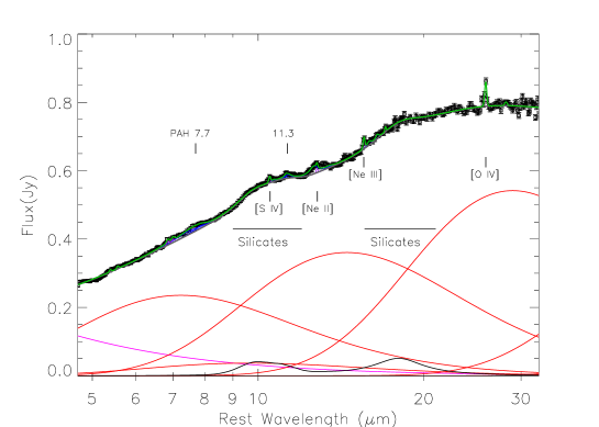
Figure 7: The best fit model (green) to the low resolution Spitzer IRS spectrum ($\times 1.077$) showing all contributions (black body continua, silicate, PAH, starlight, and narrow-emission lines). To contrast, grey curve shows contribution from black bodies, starlight, and silicate; additional contribution from PAH emission (blue), and narrow-emission lines [S iv], [Ne ii], [Ne iii] and [O iv] (purple) are also shown. Model components contributing to the aforementioned include silicate emission (bottom, black) superimposed on a black body continuum (red) and hot dust or starlight (magenta; note that it is not possible to distinguish the two without observations at near-IR wavelengths). The best fit silicate emission temperature is $\sim 160$ K while the continuum components have temperature range $50-400$ K. (The T=25K continuum component has negligible contribution to the fit and hence not shown as part of the model here.)

Table 6: Mid-IR emission lines in IRAS13349+2438

Featurea	$\lambda_{\rm rest}$b	$\lambda_{\rm vac}$c	$\mathring{W}$d	FWHMe	Fluxf
	($\mu$m)	($\mu$m)	($\times 10^{-3}$ $\mu$m)	($\times 10^{-2}$ $\mu$m)	($\times 10^{-21}$ W cm-2)
PAH(+H i?)	7.678$\pm$0.007	7.700	4.91$\pm$0.99	15.27$\pm$0.10	11.87$\pm$2.40
$[$S iv]	10.506$\pm$0.001	10.511	2.35$\pm$0.14	4.61$\pm$0.73	4.98$\pm$0.23
PAH(+H i+He ii+Mg2SiO4?)	11.243$\pm$0.001	11.250	5.14$\pm$0.95	16.14$\pm$0.09	7.97$\pm$1.41
PAH(+H i?)	12.686$\pm$0.003	12.700	0.99$\pm$0.31	2.47$\pm$0.26	1.17$\pm$0.37
$[$Ne ii$]$	12.819$\pm$0.001	12.813	3.15$\pm$0.40	3.10$\pm$0.14	3.51$\pm$0.48
PAH(+H i?)	14.241$\pm$0.006	14.250	3.24$\pm$1.75	4.62$\pm$0.82	1.04$\pm$0.74
$[$Ne v$]$	14.323$\pm$0.003	14.322	2.96$\pm$0.53	7.29$\pm$0.39	3.30$\pm$0.52
$[$Ne iii$]$	15.560$\pm$0.002	15.555	3.39$\pm$0.61	1.96$\pm$0.13	2.48$\pm$0.54
$[$S iii$]$	18.726$\pm$0.001	18.713	5.08$\pm$0.46	4.94$\pm$0.14	3.73$\pm$0.32
$[$Ne v$]$	24.317$\pm$0.009	24.318	4.65$\pm$1.86	8.30$\pm$1.02	2.23$\pm$0.80
$[$O iv$]$	25.906$\pm$0.002	25.890	28.35$\pm$3.10	5.92$\pm$0.23	9.43$\pm$1.16

^aFeature’s name
^bMeasured wavelengths (Rest frame)
^cLaboratory wavelengths (Vacuum)
^dEquivalent widths
^eFull-width at half-maximum
^fFlux

3.4.1 The Low Resolution Spectrum

We fit the low-resolution spectrum using the IDL $\chi^{2}$-fitting routines PAHFIT (Smith et al., 2007) and MPFIT (Markwardt, 2009), modified to include a silicate emission component. The continuum model consists of 6 fixed-temperature blackbody dust emission components ($T=25,50,100,200,300,400$ K) and a blackbody stellar component (5000 K). The silicate emission is modeled as the product of a Galactic silicate opacity curve (Smith et al., 2007) and a single-temperature blackbody. This assumes that the silicate emission features come primarily from an optically thin region. The flux ratio of the 10 $\mu$m–to–18 $\mu$m silicate features depends strongly on temperature, as does the shape of the 10 $\mu$m feature. The best-fit temperature for the silicate emission is $\sim 200$ K. Adding additional temperature components did not improve the fit.

The silicate emission temperature is considerably lower than the sublimation temperature ($\sim 1400$ K). This is not surprising since the silicate emission features are emitted preferentially over a temperature range of $\sim 100-200$ K. The presence of dust at temperatures up to (and possibly exceeding) 400 K is indicated by the blackbody components of our continuum model. Keck optical interferometry at $K$-band suggests near-IR emission from an inner radius of $0.92\pm 0.06$ pc (Kishimoto et al., 2009), reasonably consistent with dust at temperatures near sublimation. The peak of the SED (in $\nu F_{\nu}$) occurs at $\sim 20\mu$m, corresponding to a temperature of $\sim 200$ K. However, with a clumpy dust distribution, the bulk of this dust emission may still come from a region close to the sublimation radius.

3.4.2 The High Resolution Spectrum

Figure 8: High resolution Spitzer IRS LH (bottom panel) and SH (top panel) spectra of IRAS 13349. The spectrum shows dust features attributed to 10$\mu$m (broad continuum bump from $9-13\mu$m) and $18\mu$m emission from dust in silicates. The $18\mu$m is so broad that it is difficult to distinguish from a blackbody peaking at 200 K.

Dust signatures include a strong mid-IR excess and emission features pointing to PAHs. However, it should be noted that while we have identified the 11.2$\mu$m  feature with PAH, additional contributions from H and/or Mg-rich olivines (e.g. forsterite, Mg₂SiO₄; see Markwick-Kemper et al. 2007) are also a possibility. Detailed modeling to determine the relative contributions of PAH to Mg-rich olivines (if they exist in IRAS 13349) is beyond the scope of this paper, however.

In addition to dust features, low-equivalent width, narrow forbidden emission lines from a range of ionisation states of O, Ne, and S are detected (see Table 6 and Figure 8). In particular, the $[$NeV$]$ and $[$OIV$]$ lines originate from gas that is highly photoionized by the UV continuum from the AGN. Moreover, the $[$Ne iii$]$, $[$Ne ii$]$, and $[$S iii$]$ lines are likely dominated by AGN emission, although there may be contribution from star-forming regions.

Tommasin et al. (2010) presented a comprehensive mid-IR high-resolution spectroscopic survey of 91 Seyfert galaxies and derived useful observational and semi-analytical diagnostics that we also use here to assess the degree to which IRAS 13349 is AGN- or starburst-dominated. In particular, a good tracer of AGN contribution can be found in a comparison of the $[$Ne v$]$14.32$\mu$m : $[$Ne ii$]$12.81$\mu$m ratio against $[$O iv$]$24.32$\mu$m : $[$Ne ii$]$12.81$\mu$m. – For IRAS 13349, these values are respectively $0.800\pm 0.223$ and $2.958\pm 0.322$, pointing to an 80–90% AGN contribution to the IRAS 13349 IR emission, according to Fig. 8a of Tommasin et al.

4 The IRAS 13349+2438 Spectral Energy Distribution and its influences on the warm absorber: Observations and Theory

In having considered the line detections separately in the different wavebands, here we assess the IRAS 13349 warm absorber based on photoionisation modeling as tied to this QSO’s SED. In particular, we investigate the impact of different SED components (including the X-ray Compton power-law component, soft excess, and big blue bump/accretion disk) spanning UV to X-rays on affecting warm absorber thermodynamic stability conclusions. We also investigate the methods for assessing the IRAS 13349 black hole mass and accretion rate based on the shape of the SED.

4.1 The Observed Spectral Energy Distribution of IRAS 13349+2438

To assess photoionization scenarios for the absorbing gas in IRAS 13349, we first need to know the intrinsic spectral energy distribution (SED) of the active nucleus that is illuminating the surrounding gas and dust. To start, we assemble an IR to X-ray SED based upon our observations and archival data (see Figure 9). In the IR, we start with 170 $\mu{\rm m}\;$far IR ISOPHOT measurements (Spinoglio et al., 2002), while mid-IR (12, 25 and 60 $\mu\rm m$) IRAS data are taken from the Faint Source Catalog of Moshir et al. (1990), and near-IR photometric points are the 2MASS 1–2 $\mu{\rm m}\;$data from the Large Galaxy Atlas of Jarrett et al. (2003). For comparison, our Spitzer IRS spectrum is overlaid on these data after scaling to match the 12 $\mu{\rm m}\;$and 25 $\mu{\rm m}\;$IRAS photometry (as noted in §2.4). In the optical and UV bands, we correct our observed HET and HST spectra for foreground Galactic extinction of $E(B-V)=0.013$, which we obtain from NED, assuming a mean Galactic extinction curve (Cardelli et al., 1989) with a ratio of total to selective extinction of $R_{V}=3.1$. Our Chandra  spectrum in the X-ray is corrected for foreground Galactic absorption as described in §2.

For comparison, we generate a “generic” composite optical-UV QSO spectrum based on the Sloan Digital Sky Survey (SDSS) composite quasar spectrum of Vanden Berk et al. (2001) (for $\lambda>3200$ Å  rest) and the radio-quiet HST composite quasar spectrum of Telfer et al. (2002) at shorter wavelengths. If we normalise this composite spectrum to match our extinction-corrected HET spectrum at 5700 Å rest (resulting in the solid blue curve of Figure 9; hereafter “5700Å -normalised-generic-composite”) what immediately stands out is the large deficit of UV and far UV flux in IRAS 13349, which is likely reradiated by heated dust in the IR since the observed SED peaks at 30 $\mu$m, rest. In the optical band, the HET spectrum of IRAS 13349 is virtually identical to that of the SDSS composite portion of the 5700Å -normalised-generic-composite, indicating that the IRAS 13349 optical spectrum is only modestly reddened or extincted at these wavelengths. (The analysis of Hopkins 2004 shows that the full SDSS composite has an internal SMC-like extinction of $E(B-V)\sim 0.013$ at most.) The Balmer decrement measured in our HET data is $2.85\pm 0.18$ for the ratio of H$\alpha$–to–H$\beta$. Correcting this for foreground extinction, it becomes $2.817\pm 0.18$. To correct this to a nominal Case B value of 2.76 implies $E(B-V)=0.021$ for an SMC-like extinction law. Comparing the Galactic-extinction-corrected spectrum of IRAS 13349 to the SDSS composite in more detail, the ratio (in the continuum) is flat from 4000–6000 Å; if anything, IRAS 13349 appears a bit bluer. So, internal extinction on the order of 0.01 to 0.02 (with an SMC-like law) is consistent with $E(B-V)=0.021$ as derived from the Balmer decrement. – For this value, $A_{\rm V}={\rm E(B-V)}R_{\rm V}=0.09\pm 0.02$ taking $R_{V}=4.05\pm 0.8$ ala Calzetti et al. (2000).

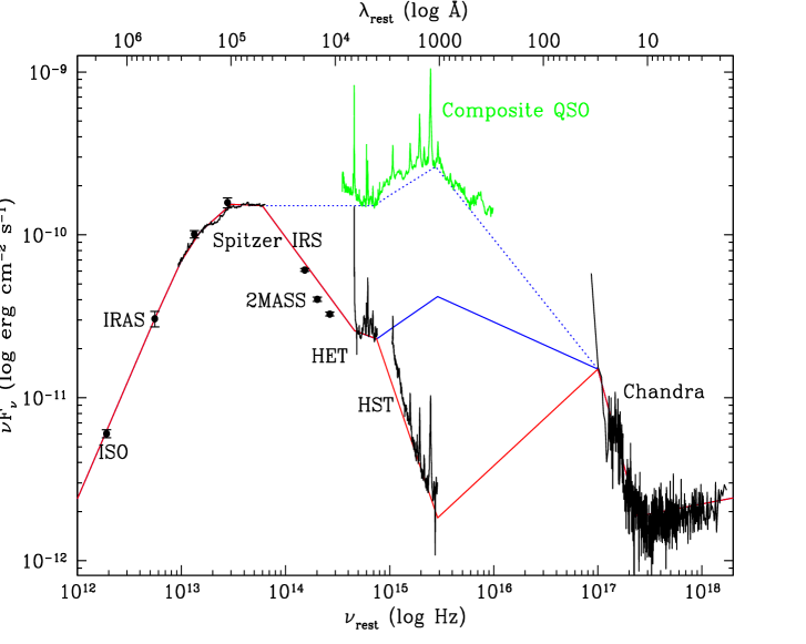
Figure 9: Observed and intrinsic Spectral Energy Distribution (SED) of IRAS 13349 based on our observations. The x axis (both $\nu$ and $\lambda$) is in the rest frame. Solid points with error bars are archived data from (1) ISO 170$\mu$m data from Spinoglio et al. (2002), as labeled. (2) IRAS 12, 25, 60 $\mu$m measurements of the IRAS Faint Source Catalog, Version 2.0 $-$Moshir et al. 1990, and (3) 2MASS Large Galaxy Atlas of Jarrett et al. 2003. Spectra are also shown (in solid black) of recent observations with the Spitzer IRS (IR), the HET (optical), the HST STIS (UV), and the Chandra HETGS (X-ray). The “Composite QSO” spectrum (solid green line) has been renormalised upward by 0.85 dex so that its EUV peak lies 0.25 dex above the IR peak of the observed IRAS 13349 spectrum, as is found in the mean RQ QSO spectrum of Elvis (1994). Straight line segments between $10^{15}$ Hz and $10^{17}$ Hz show a range of simple assumptions for what the IRAS 13349 SED can be in the EUV energy range where there is no data. At one extreme, we take our observed SED without any corrections and decompose it into a set of power-law segments connecting the observed HST spectrum to the lowest ($\sim$0.3 keV, rest) energy Chandra point (solid red). The solid blue line represents a “corrected” UV spectrum where the “correction” is derived by assuming that the intrinsic spectrum is represented by the Composite QSO spectrum normalised to the observed HET spectrum of IRAS 13349 assuming a break at the peak of the Composite spectrum (1000 Å rest) that we again extrapolate down to $\sim$0.3 keV in the X-ray. The dotted blue line follows the continuum established by the Composite spectrum renormalised by the relative UV and IR peaks of the Elvis (1994) mean RQ QSO SED, which we again extrapolate through the EUV using a power law from the peak of the Composite spectrum at 1000 Å to the Chandra  0.3 keV soft X-ray point.

Based on the 5700Å -generic-normalised-composite spectrum we find that the UV/optical peak (i.e. the peak of the solid blue SED) is 0.6 dex below the peak radiation in IR (at $\sim 10^{5}$ Å). According to the median radio-quiet QSO SED in Figure 12 of Elvis (1994), the UV peak for a “normal QSO” should be 0.25 dex above the IR peak. Assuming IRAS 13349 to be in this category (IR and optical spectra suggest this to be the case for IRAS 13349) its UV/optical peak is then 0.85 dex below that of an unabsorbed “normal QSO”. This suggests that either we are viewing the optical spectrum of IRAS 13349 through a gray screen, or largely in scattered light, but from a scattering region that again is largely colour neutral at wavelengths longward of 4000 Å. At shorter wavelengths, the observed UV spectrum is likely some complex mix of scattered and absorbed light from the central regions. The complex geometry of this radiative transfer is difficult to unravel even using the added benefit of polarisation information (W92; Hines et al., 2001), so to produce an SED that is fully corrected for these effects, we will assume that scaling the composite QSO spectrum to the level implied by the median QSO SED in Elvis (1994) is a good representation of the intrinsic SED of the active nucleus of IRAS 13349. The resultant SED (see Fig. 9, solid green and associated dotted blue line connecting it to the IR and X-rays) looks like a qualitatively good description for the intrinsic SED of IRAS 13349 since the extreme ultraviolet portion of the composite spectrum is declining smoothly to higher frequency in a way that would provide a good match to the soft X-ray portion of the spectrum observed with Chandra . Assuming this to be the intrinsic IRAS 13349 spectrum, at its corrected UV luminosity of $L_{2500}=8.1\times 10^{29}~{}\rm ergs~{}s^{-1}~{}Hz^{-1}$, we derived $\alpha_{ox}=-1.83$, a value that is $-0.25$ lower than the nominal $\alpha_{ox}=-1.58$ value expected from the Young et al. (2010) relation. This slightly lower $\alpha_{ox}$ we observe for IRAS 13349 is consistent with the weak C iv absorption that we see in the HST spectrum (c.f. Gallagher et al., 2006).

Table 7: Luminostiy of IRAS 13349+2438 in different energy bands

SED	e $\rm L_{bol}$	f $\rm L_{IR}$	g $\rm L_{Opt}$	h $\rm L_{UV}$	i $\rm L_{EUV}$	j $\rm L_{X}$
	($\rm\times 10^{46}erg\,s^{-1}$)	($\rm\times 10^{46}erg\,s^{-1}$)	($\rm\times 10^{45}erg\,s^{-1}$)	($\rm\times 10^{45}erg\,s^{-1}$)	($\rm\times 10^{45}erg\,s^{-1}$)	($\rm\times 10^{44}erg\,s^{-1}$)
a 1	1.42	1.19	0.72	0.36	0.68	5.55
b 2	1.74	1.19	0.72	1.44	2.77	5.55
c 3	3.90	1.51	3.72	9.73	9.89	5.55
d 4	2.03	-	1.95	9.60	7.19	5.42

^aObserved SED - the solid red line in Figure 9.
^bCorrected SED - the solid blue line in Figure 9 and in all panels of Figure 10.
^cCorrected SED - the dotted blue line in Figure 9 and in all panels of Figure 10.
^dTheoretical SED - the solid red line in bottom panel of Figure 10.
^eBolometric luminosity integrated from $\rm log\,\nu=11.5-20$.
^fIR luminosity integrated from $\rm log\,\nu=11.5-14.5$.
^gOptical (HET) luminosity integrated from $\rm log\,\nu=14.5-14.87$.
^hUltraviolet (HST) luminosity integrated from $\rm log\,\nu=14.87-15.5$.
ⁱExtreme ultraviolet (unobserved) luminosity integrated from $\rm log\,\nu=15.5-17.0$.
^hX-ray luminosity integrated from $\rm log\,\nu=17.0-20$.

We have also checked the Elvis et al. SED against more recent compilations of QSO SEDs (Shang, 2011; Richards et al., 2006; Hopkins et al., 2007) built from various combinations of SDSS, Spitzer, FUSE, and HST data. The variation in the UV-IR peak difference (in $\rm log(\nu F_{\nu})$) is less than a factor of 2 when comparing these different samples. (Note that the Hopkins et al. SEDs use the Richards et al. sample of objects but adds an additional $\alpha_{\rm ox}$ correction based on the object’s peak UV flux; also, the Richards sample of QSO, in using primarily SDSS have a median redshift $z>0.5$).

To assess luminosity contributions for the different wave band components of these SEDs, we integrate the line-segment SEDs of Figure 9 over the energy bands noted in Table 7; we assume $H_{0}=73$ km s^-1 Mpc^-1, $\Omega_{\rm M}=0.25$, and $\Omega_{\Lambda}=0.75$. These luminosities are then used as relevant for calculations in subsequent sections, either in whole or in part. The bolometric luminosity we derived from the piecemeal integration is $L_{\rm bol}\sim 3.12\times 10^{46}~{}\hbox{${\rm\thinspace erg}{\rm\thinspace s}^{-1}\,$}$.

4.2 Reconstruction of the UV to X-ray SED and its components: theory and observations

The radiation from the central regions of AGN is likely to peak in the extreme ultraviolet at $\sim 10-100\,{\rm eV}$ ($\sim 124-1240$ Å), an energy range often suffering from extinction effects due to Galactic and/or intrinsic dust. As stated in §4.1, such is the case for IRAS 13349, which shows a large UV and far-UV deficit in its observed SED, which we attribute to dust extinction, a conclusion also supported by Spitzer IR observations (see §3.4.1 for details). Likewise, the two most important spectral components featuring in this un-observable energy range are the disc blackbody from an accretion disc peaking between 10 - 100 eV (typical of AGN), and the soft excess, typically manifesting at $<$ 1 keV. Here, using theoretical considerations in combination with our multi-waveband observations of IRAS 13349, we derive what we believe to be the most likely scenario for the intrinsic IRAS 13349 SED, sans extinction.

The ionising continuum dictating the ionisation state of the absorbers in AGN is primarily contained in the UV-to-X-ray range. Therefore we focus our discussion on this energy range, with special attention paid to recreating the extincted UV part of the spectrum.

The general mathematical form we use in building the IRAS 13349 theoretical SED is:

$$f(\nu) \sim \Big{[}A_{pow}\,\nu^{-\alpha}+A_{se}\,\left\{\frac{2\,\pi\,h}{c^{2}}\,\frac{\nu^{3}}{\exp(h\,\nu/k_{B}\,T_{se})\,-\,1}\right\}$$

$$~{}~{}~{}~{}~{}~{}~{}~{}~{}~{}~{}~{}~{}~{}~{}~{}~{}~{}~{}~{}~{}~{}~{}~{}+A_{dbb}\,f_{dbb}(\nu,T_{in})\Big{]}e^{-\frac{\nu}{\nu_{max}}}~{}~{}~{}~{}~{}~{}~{}~{}~{}\rm{(a)}$$

$$f(\nu) \sim \Big{[}A_{pow}\,\nu^{-\alpha}+A_{se}\,f_{c}(\nu,T_{in},T_{c},\Gamma_{c})$$

$$~{}~{}~{}~{}~{}~{}~{}~{}~{}~{}~{}~{}~{}~{}~{}~{}~{}~{}~{}~{}~{}~{}~{}~{}+A_{dbb}\,f_{dbb}(\nu,T_{in})\Big{]}e^{-\frac{\nu}{\nu_{max}}}.~{}~{}~{}~{}~{}~{}~{}~{}~{}\rm{(b)}$$

where the first and third terms in both Equations LABEL:eqn:theoryseda and LABEL:eqn:theorysedb represent the 1-10 keV X-ray power-law and the big blue bump (modeled by “disk-blackbody”) respectively. As can be seen, the two equations differ only in the 2nd term, associated with competing models describing the soft excess (see §4.2.1 for details). We proceed with a discussion of this component, to be followed by more in-depth discussion of the big blue bump: its derivation, and the dependence of its shape on the central black hole mass and accretion rate.

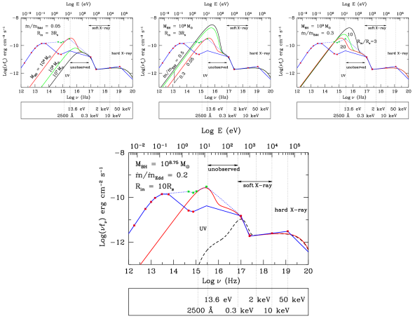
Figure 10: Theoretical SEDS calculated for IRAS 13349 based on multi-wavelength data shown in Fig. 9. The filled red squares reflect the observed IRAS 13349 SED based on ISO, IRAS, Spitzer, HET and Chandra. Green squares are the renormalised observed “generic-composite QSO” spectrum made up of a SDSS composite of $\sim 2000$ quasars (Vanden Berk et al., 2001) longward of 3200 Å and the HST RQ quasar composite of Telfer et al. (2002). The solid and dotted blue lines trace out the same SED as in Fig. 9. (BOTTOM PANEL:) The theoretically computed SED (solid red) that best matches the observed IRAS 13349 SED corresponds to a black hole mass of $\rm{M_{BH}}\approx 10^{8.75}\,\rm{M_{\odot}}$, an accretion rate of $\rm{\dot{m}/\dot{m_{Edd}}}\approx 0.2$ and $R_{in}=10R_{s}$. On the other hand, if the accretion disc is completely ignored and one draws a SED based only on the Chandra-HETG spectra, we get the dashed black curve. (TOP PANELS:) Theoretical SEDs comparing spectral shape differences for different combinations of $\rm{M_{BH}}$, $\rm{\dot{m}/\dot{m_{Edd}}}$ and $R_{in}/R_{s}$ as discussed in Section 4.2, for comparison and edification.

4.2.1 The sub-keV soft excess

Observations of most AGN reveal that the SED between 2-10 keV is well approximated by a power-law with spectral indices $\alpha\sim 0.9$ (photon indices $\Gamma\sim 1.9$). However, if this power-law is extended to lower energies ($<1\,{\rm keV}$), for most type I AGN, there is additional unaccounted radiation, which has come to be known as the soft excess. This component is particularly important for shaping the nature of the X-ray absorber (Chakravorty et al., 2012). However, the physical origin of the soft excess is not understood, and presently the community largely treats it as a phenomenological spectral component modeled as a blackbody (Equation LABEL:eqn:theoryseda) with temperature $T_{se}\sim 100-200\,{\rm eV}$, which generally does a good job of describing most observations. Since this temperature is too hot for the temperature, $T_{in}$, of the innermost stable circular orbit of the accretion disc in AGN (see Equation 2), the soft excess is often believed to be a separate spectral component altogether, or a reprocessed (shortward in wavelength) extension of the accretion disc component. Our fit to the Chandra HETGS spectrum of IRAS 13349 in §3.1 gives a temperature for the soft excess of $T_{se}=99$ eV.

An alternative model $f_{c}(\nu)$ (Equation LABEL:eqn:theorysedb) for the soft excess is the thermal Comptonisation model nthcomp (Lightman & Zdziarski, 1987; Zdziarski et al., 1996; Życki et al., 1999) included in xspec v.12.5 (Arnaud, 1996). In this description, the seed photons from the accretion disc are reprocessed by the thermal plasma to generate sufficient photons at sub-keV energies to mimic the soft excess. The high energy cut-off of this component is parametrised by the electron temperature $T_{c}$, and the low energy rollover is dependent on the effective temperature, $T_{in}=T(R_{in})$ (Equation 2) of the seed photons from the accretion disc. Between the low and high energy rollovers, the shape of the spectrum is approximated by an asymptotic power-law with photon index $\Gamma_{c}\approx\frac{9}{4}y^{-2/9}$, where $y$ is the Compton y-parameter, which gives a measure of the extent of Compton reprocessing; i.e., the larger the value of $y$, the greater the fraction of photons reprocessed from the accretion disc. For our modeling efforts, we adopt $T_{c}=T_{se}=100$ eV, consistent with our Chandra soft X-ray data for IRAS 13349. The associated normalisation constant $A_{se}$ was determined from the ratio of the $35-5$ Å  (0.35 - 2.5 keV) photon flux in the soft excess component to that in the power-law, as seen in the Chandra HETGS data for IRAS 13349.

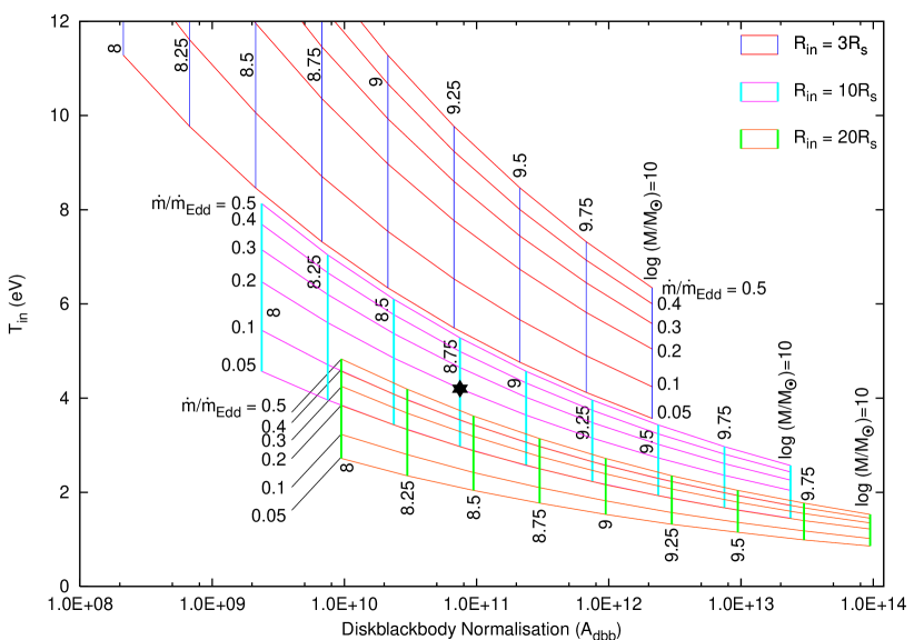
Figure 11: Based on grid runs using diskbb, a theoretical representation of all the SEDs that we have investigated to find the black hole parameters that best match the composite QSO spectra normalised to the flux of IRAS 13349. The big blue bump SED can be mathematically described by $T_{in}$ and $A_{dbb}$ which we plot for each combination of the parameters $\rm{M_{BH}}$, $\rm{\dot{m}/\dot{m_{Edd}}}$ and $R_{in}$. The three different grids (colour coded and labeled appropriately) of $\rm{M_{BH}}$ and $\rm{\dot{m}/\dot{m_{Edd}}}$ correspond to three values of $R_{in}/R_{s}$. The black star represents the best match SED (red curve, lower panel of Figure 10) for $\rm{M_{BH}}\approx 10^{8.75}\,\rm{M_{\odot}}$, an accretion rate of $\rm{\dot{m}/\dot{m_{Edd}}}\approx 0.2$ and $R_{in}=10R_{s}$. See Section 4.2.3 for details.

The aforementioned models of the soft excess do not influence the UV part of the spectrum and hence do not affect the predictions for the shape of the big blue bump (see next section). The soft excess is an important component influencing the ions which absorb the soft X-ray radiation. Our theoretical simulations show that there is a slight difference in the predicted ion fraction of the various soft X-ray ions, depending on choice of models for the soft excess. However, while the Chandra HETGS data cover the energy range of the soft excess, these are not sensitive enough to detect these relatively small differences in ion abundances, and hence cannot be used to differentiate between the nthcomp or blackbody models. Therefore, for the remainder of our analysis we adopt the nthcomp model with $\Gamma_{c}=2.3$ and $T_{c}=100\,{\rm eV}$, acknowledging that an alternative blackbody model with $T_{se}=100\,{\rm eV}$ is likely to produce equally good results.

4.2.2 The “Big Blue Bump”

Multi-wavelength observations suggest that AGN continua peak in the EUV energy band and usually dominate the quasar luminosity (e.g., Elvis 1994). This spectral component, often referred to as the “Big Blue Bump”, is considered to be the signature of the presence of an accretion disc. Yet, for many systems, it can only be partially observed in the UV-EUV energy range. As such, an attempt to reconstruct it requires careful theoretical considerations.

According to standard thin disc accretion theory (Shakura & Sunyaev, 1973), radiation from the accretion disc may be modeled as a sum of local blackbodies emitted from the different annuli of the disc at different radii, the temperature of the annulus at radius $R$ being

$$T(R)=6.3\times 10^{5}\left(\frac{\dot{m}}{\dot{m}_{\rm Edd}}\right)^{\frac{1}{4}}\left(\frac{M}{10^{8}M_{\odot}}\right)^{-\frac{1}{4}}\left(\frac{R}{R_{s}}\right)^{-\frac{3}{4}}\rm{K}$$ (2)

(Peterson, 1997; Frank et al., 2002) where $\dot{m}$ is the accretion rate of the central black hole of mass $M_{BH}$, $\dot{m}_{\rm Edd}$ is its Eddington accretion rate and $R_{s}$ is the Schwarzschild radius. The normalisation constant $A_{dbb}$ for this spectral component is given by

$$A_{dbb}=\left\{\frac{R_{in}/\rm{km}}{D/(10\,\,\rm{kpc})}\right\}^{2}\cos\theta$$ (3)

for an observer at a distance $D$ whose line-of-sight makes an angle $i$ to the normal to the disc plane. $R_{in}$ is the radial distance of the innermost stable annulus of the accretion disc from the black hole. Thus, the radiation from the accretion disc has direct dependence on the mass of the black hole and its accretion rate. As such, the shape of the spectral energy distribution can provide important diagnostic power for assessing the fundamental parameters of the black hole.

We acknowledge that more rigorous models exist for modeling the big blue bump, that involve real radiative transfer in the accretion disc (see e.g. Blaes et al. 2001; Hubeny et al. 2000, 2001; Hui et al. 2005) and/or the black hole spin effects (see e.g. Davis et al. 2005; Davis & Hubeny 2006). For the same black hole mass and accretion rate, relative to a simple “disk-blackbody”, these more-involved models change the location of the peak and the shape of the EUV spectrum, as UV and EUV flux gets absorbed and re-emitted at longer wavelengths in these models. For models which include the black hole spin, the peak of the accretion disk spectrum is pushed to higher energies for increasing black hole spin. Thus, qualitatively we can expect that using these models would result in higher black hole mass as compared to the best-fit results obtained by using “disk-blackbody”, for the same accretion rate. However, since the UV spectrum of IRAS 13349 is heavily extincted, we cannot make observationally based distinctions between the different accretion disc models. Given this, in the next section we opt for the less-computationally expensive “disk-blackbody” model (Mitsuda et al., 1984; Makishima et al., 1986) to assess the mass and accretion rate of the black hole. While we present results based on fits to diskbb to allow for easier comparison to work on this and other AGN by other authors, we acknowledge that the model ezdiskbb (Zimmerman et al., 2005) may be the theoretically more sound model, and therefore also discuss our subsequent SED results based on a comparison of the two, where relevant. In brief, the major difference in the two models is most notable at $R<10R_{\rm in}$, whereby the diskbb predicted temperature continues to increase in contrast to ezdiskbb; this difference stems primarily from the ezdiskbb imposed boundary condition that the viscous torque be zero at the inner edge of the disc.

4.2.3 Determining the mass and accretion rate of the IRAS 13349 black hole

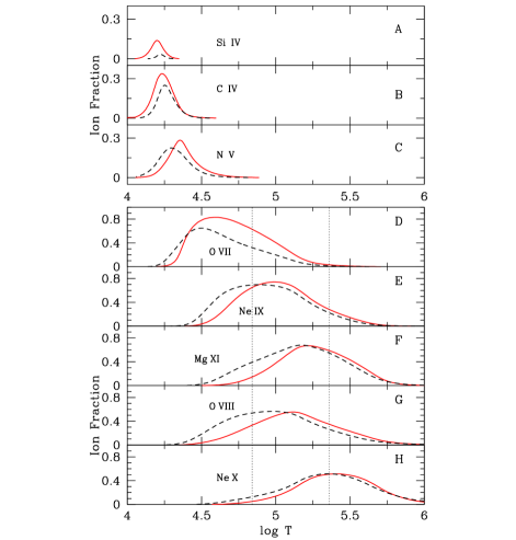
Figure 12: Ion fractions versus gas temperature as a function of the two relevant ionising SEDs. The line styles follow the same scheme used in Figure 10 : the solid red curves are obtained using the full UV to X-ray SED whereas the dashed black curves are a result of an X-ray only SED based on only the Chandra-HETG continuum. The panels A-C are for the UV ions and D-H are for the X-ray ions as labeled. The dotted vertical lines running across panels D-H mark the range $2.0\leq\log\xi\leq 3.0$ corresponding to the full UV to X-ray ionising SED. This is the range of $\xi$ within which the ion fractions for Ne ix, Mg xi and O viii peak. The importance of this range of the ionisation parameter is discussed in Sections 4.3 and 5.1.

Using the observed IRAS 13349 SED (see §4.1 discussion), in combination with Equation LABEL:eqn:theorysed, and the Shakura & Sunyaev (1973) model (applied to Equation LABEL:eqn:theorysed, 3rd term), we generate a series of SEDs for different values of $\dot{m}$ and $M_{\rm BH}$ to obtain the best match to the IRAS 13349 SED (Figure 9; §4.1 for details). We carry out an iterative, step-by-step approach to reconstruct the UV-EUV SED, with permutations of the relevant parameters, as described below.

We begin by running models using a coarse grid of various combinations of the parameter values $\rm{\dot{m}/\dot{m}_{\rm Edd}}=(0.05,0.1,0.5,1.0)$ and $\rm{M_{BH}}=(10^{7},10^{8},10^{9}\,\rm{M_{\odot}}$ for each $\rm{\dot{m}/\dot{m}_{\rm Edd}}$,) with a fixed $R_{\rm in}=3R_{\rm S}$. For this initial run, we find that $\rm{\dot{m}/\dot{m}_{\rm Edd}}=0.05$ and $\rm{M_{BH}}=9.0$ gives a reasonable match to the observed IRAS 13349 SED (see top left panel of Figure 10 comparing theoretical models with UV composite QSO spectra, green data points). It should be noted that we can expect a range of acceptable matches between theory and observations for different permutations of key parameters, primarily due to the fact that Equation LABEL:eqn:theorysed, which we use for modeling the big blue bump, is degenerate between mass and accretion rate. The top panels of Figure 10 demonstrate the effects on the shape of the theoretical SED when various combinations of $R_{\rm in}$, $\rm M_{BH}$, and $\rm{\dot{m}/\dot{m}_{\rm Edd}}$ are fixed/varied.

Therefore, to reduce uncertainties, we use a black hole mass derived from the H$\beta$ line width ($\sigma_{\rm H\beta}=1948~{}\pm 3.7\hbox{${\rm\thinspace km}{\rm\thinspace s}^{-1}\,$}$; see Section 3.3), and the optical continuum luminosity $\lambda L_{5100}=6.28\times 10^{44}~{}\rm erg~{}s^{-1}$, based on the renormalised, green Composite QSO spectrum in Figure 9. Based on the McGill et al. (2008) relation,

$$\rm log\,M_{BH}=7.68+2\,log\,\frac{\sigma_{\rm H\beta}}{1000}~{}\hbox{${\rm\thinspace km}{\rm\thinspace s}^{-1}\,$}+0.518\,log\,\frac{\lambda L_{5100}}{10^{44}}~{}erg~{}s^{-1}$$ (4)

we derive for IRAS 13349, $\rm log~{}M_{BH}=9.10~{}M_{\odot}$; the McGill relation has an rms scatter in $\rm log~{}M_{\rm BH}=0.09$. Barring better constraints, we use $\rm M_{BH}\sim 10^{9}~{}\rm M_{\odot}$ for input into Equation LABEL:eqn:theorysed to determine the accretion disc component of our theoretical intrinsic SED. Given that this $M_{\rm BH}$ estimate is close to our “best fit” value from the initial coarse grid of runs based on a fixed $R_{\rm in}=3R_{\rm S}$, we next run a finer grid of models allowing all the aforementioned three parameters free. Figure 10 (bottom panel) shows the best theoretical SED match (red curve) to the UV-EUV flux distributions based on our hypothesised extrapolation of observed data in the UV-EUV spectral domain (green points). The best match SED has optimal parameters $\rm M_{BH}=10^{8.75}M_{\odot}$, $\rm{\dot{m}/\dot{m}_{\rm Edd}}=0.2$, and $R_{\rm in}=10R_{\rm S}$. Figure 11 shows $T_{in}$ versus $A_{dbb}$ for all theoretical values of $M_{\rm BH}$, $\rm{\dot{m}/\dot{m}_{\rm Edd}}$ and $R_{\rm in}$ that we have investigated, including where in these curves our best fit lies. For thoroughness, we also perform the same exercise using ezdiskbb, and find that while the “best fit” SED shape remains the same, the same exercise with ezdiskbb gives a higher accretion rate for fixed values of $R_{\rm in}$ and $M_{\rm BH}$. From our trials at finding the best match based on ezdiskbb, the relevant SED parameters bracket a similar best range found using diskbb, i.e. $10^{8.50}<\rm M_{BH}<10^{9.25}M_{\odot}$, $0.2\leq\rm{\dot{m}/\dot{m}_{\rm Edd}}\leq 0.7$, and $3<R_{\rm in}\leq 10R_{\rm S}$.

The shape obtained for the big blue bump is then complemented with X-ray power-law ($\S\ref{sec:uvxsed}$), and soft excess (discussed in §4.2.1) components to derive the full UV-XRay SED (Figure 10 bottom panel - red) needed for input to photoionization modeling.–See luminosity information associated with SED #4 of Table 7. (Note that $L_{\rm IR}$, which is primarily attributed to reradiation by dust that has absorbed part of the optical-UV radiation is excluded here, since it has no bearings on the actual disc spectrum.) Note that if the accretion disc component is completely ignored and a SED is constructed on the basis of only the Chandra HETGS X-ray data for IRAS 13349, then one would obtain the black dashed curve shown in the bottom panel of Figure 10. Such an SED was used by Holczer et al. (2007) to study the warm absorber in IRAS 13349. In Sections 4.2.4 and 5.1, we discuss differences in, and effects on, derived absorber properties based on an ionising SED that accounts for only X-ray contributions versus one which also includes disc contributions.

4.2.4 Advantages to using the full UV to X-ray SED for assessing the location(s) of the absorbing gas

Approximately half of all low-z AGN show high-ionisation UV absorption lines and signatures of even higher ionisation warm absorption in the X-ray data. In assessing the role of the disc ionising radiation for affecting our conclusions on UV and X-ray warm absorber properties (e.g. common versus distinct origins; continuous vs. clumpy clouds), we use xstar to generate ion fractions (Figure 12) as a function of the temperature of the absorbing gas for the UV (panels A-C) and the X-ray (panels D-H) ions, using an SED that includes the big blue bump, the sub-keV soft excess and the X-ray power-law (Figure 10 lower panel - red curve) versus an SED that only accounts for the X-ray spectral components, namely the power-law and the black body soft excess, as determined from continuum fits to the X-ray data (Fig. 10 black dashed curve).

One of the most important ions in the X-ray warm absorber is He-like O vii. As can be seen in Figure 12, its ion fraction is under-predicted by $\sim 25\%$ if the big blue bump is excluded from the ionising continuum (panel D). The relative abundance of O vii and the H-like O viii, another of the important ions in the X-ray warm absorber, are sensitively inter-related. Hence under-prediction of the O vii ion would be associated with a complementary over prediction of the O viii (panel G). Mg xi is also significantly over-predicted by a SED which excludes the big blue bump. Furthermore, it can be seen that the inclusion of the big blue bump predicts a larger ion fraction for the UV ions (panels A-C), and hence a higher likelihood that they are produced in the same gas as that responsible for O vii (panel-D) seen in X-ray absorbers. This is contrary to the conclusions one would arrive at, if considering an X-ray-only SED.

4.3 The ionised dusty absorbers in IRAS 13349

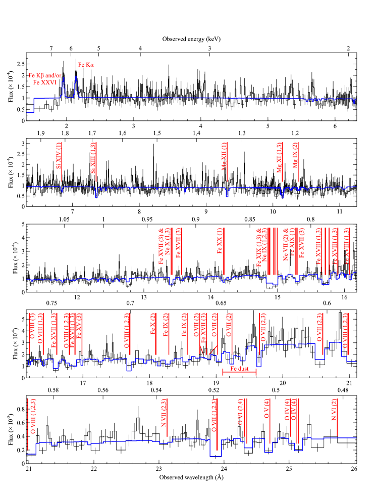
Figure 13: The best fit to the Chandra HETGS spectrum of IRAS 13349 (in the observed frame). Numbers associated with the ion labels correspond to contributions from one or multiple absorbers as described in Section 4.3 and Table 8. Note that while this figure is shown with adaptive binning ($15\,\rm cts\,bin^{-1}$) to facilitate easier viewing, our fitting results are based on constant binning at the HETGS resolution. Only predicted lines with equivalent width $W_{\lambda}>0.005$ mÅ  are labeled.

Using xstar 2.2.1, we generate “warm absorber” models with ion populations that reflect the ionising spectrum of our preferred IRAS 13349 SED (see Figure 10, bottom panel, red SED; §4.2.3 for details). We employ the analytic version of xstar which enable line broadening and optical depth calculations in real time as relevant to the data. In addition, the granularity associated with analytic models are only in $\xi$, which we mitigate by creating population files sampled with $\Delta(\log\xi)<0.1$ . (In contrast, one can expect table models to have granularity in all free parameters. – Private Communication: Tim Kallman.)

Table 8: Best fit parameters based on fits to the Chandra HETGS data.

a BB norm ($10^{-4}$)	b BB kT	c PL norm ($10^{-3}$)	d PL $\Gamma$
$\rm{ph\,cm^{-2}\,s^{-1}}$	(eV)	$\rm{ph\,cm^{-2}\,s^{-1}}$
The continuum
$1.87_{-0.07}^{+0.11}$	$107_{-0.1}^{+0.1}$	$1.30_{-0.02}^{+0.01}$	$1.98_{-0.02}^{+0.02}$
	e Line Flux ($\times 10^{-6}$)	f Centre	g Width	Width
	$\rm{ph\,cm^{-2}\,s^{-1}}$	(keV)	(keV)	(km s-1)
The Iron Emission Lines
Fe i K$\alpha$	$4.2_{-1.85}^{+0.98}$	$6.42_{-0.03}^{+0.05}$	$0.04_{-0.02}^{+0.06}$	$1868_{-936}^{+2801}$
Fe i K$\beta$ and/or Fe xxvi (?)	$4.0_{-1.86}^{+2.19}$	$7.04_{-0.04}^{+0.04}$	$0.05_{-0.05}^{+0.06}$	$2129_{-2129}^{+2555}$
	h $\rm log\,\xi$	i $\rm v_{blue}$	j $\rm b$	k $\rm N_{H}$
		(km s-1)	(km s-1)	($10^{21}\rm{cm^{-2}}$)
4 components of the warm absorber
WA-1	$1.67_{-0.12}^{+0.15}$	$-798_{-78}^{+18}$	$395_{-62}^{+59}$	$1.01_{-0.07}^{+0.13}$
WA-2	$3.38_{-0.07}^{+0.10}$	$-678_{-115}^{+68}$	$492_{-85}^{+95}$	$3.26_{-0.55}^{+0.57}$
(WA-3)	$3.00_{-0.07}^{+0.00}$	$-758_{-48}^{+71}$	$95_{-38}^{+76}$	$2.39_{-0.43}^{+0.54}$
(WA-4)	$-0.94_{-0.06}^{+0.22}$	$-1298_{-197}^{+127}$	$455_{-146}^{+315}$	$0.14_{-0.04}^{+0.05}$
	l $\rm N_{Dust}$	m $\rm v_{blue}$	$\frac{\rm N_{Dust}}{\rm N_{Gas}+N_{Dust}}$
	($10^{17}\rm{cm^{-2}}$)	(km s-1)
	Iron based Dust
	$1.23_{-0.33}^{+0.21}$	$-104_{-275}^{+407}$	98.27%

^aBlackbody normalisation. ^bBlackbody temperature. ^cPower-law normalisation. ^dPower-law photon index.
^eGaussian emission line normalisation. ^fLine central energy. ^gLine width.
^hLog of the ionization parameter (See Section 5.1 for detailed definition).
ⁱOutflowing velocity (negative indicates blushift). ^jTurbulent/thermal velocity.
^kColumn density. ^lColumn density of iron in condensed matter (i.e. dust/molecule) form. ^mDust outflow velocity (negative indicates blushift).

Using codes we developed for the isis (Houck & Denicola, 2000) fitting/analysis package in combination with the aforementioned xstar-generated models, we initially fit the data (binned to the HETGS resolution) with 9 absorber components spanning the $-4<\log\xi<4$ range, and find that it is the high $\xi$ ($\log\xi>1$) gas which drive the fit. In also investigating dustless (Section 4.3.2) and dusty (Section 4.3.3) absorption, we find that a statistically good fit describing the HETGS data (0.5–1.3 keV MEG and 1.2–8.9 keV HEG chosen to maximise both spectral resolution and throughput) is a power-law plus blackbody continuum absorbed by two ionised absorbers [hereafter WA-1 ($\log\xi=1.68_{-0.16}^{+0.14}$, $\log\rm{N_{H}}=21.03_{-0.09}^{+0.05}$) and WA-2 ($\log\xi=3.26_{-0.08}^{+0.05}$, $\log\rm{N_{H}}=21.66_{-0.06}^{+0.05}$)] at similar ($\sim$ 700–800 ${\rm\thinspace km}{\rm\thinspace s}^{-1}\,$) velocities, and iron dust (see Section 4.3.3 for details), intrinsic to the source. The reduced Cash statistic $\Delta C$ for this model is 1.147 (2887.127/2540) and the corresponding reduced $\chi^{2}$ = 1.102 (2774.783/2540). While the fit naturally tend towards the aforementioned two-absorption+dust model, we consider additional absorbers, driven by our own theory considerations based on thermodynamic stability arguments (see Section 5.1; also Section 4.3.1) and the detection of the Unresolved Transition Array in the previous XMM (Sako et al., 2001) study of IRAS 13349 (Section 4.3.2). While these additional absorbers aid in fitting a few additional weak lines, they do not add significantly to the overall improvement in fit statistics ($\Delta C$ = 2842.34/2540 = 1.133, $\chi^{2}$ = 2741.884/2540 = 1.093 for the addition of WA-3 and WA-4). – See Table 8 and Figure 13 for details on the four-absorber+dust model. We also test for the presence of additional absorbing material from within the Milky Way and find no strong evidence for its presence along the IRAS 13349 line-of-sight.

On the intrinsic IRAS 13349 absorption, Figure 14 shows the observed and predicted column densities ($N_{\rm j}\;$) of the various ions we have found in the UV and X-ray spectra of IRAS 13349+2438, based on both the plasma diagnostic approach of Sections 3, and the xstar photoionization fitting here. As demonstrated in the figure, the series fitting and xstar modeling agree with each other on the predicted column densities for many of the detected ions. For instance, it can be seen that for O vii (Figure 14, left panel A), the column density predicted from fitting the line series (horizontal shaded regions) matches with the xstar predicted $N_{\rm j}\;$. In addition, the figure is instructive in revealing the extent to which each absorber is responsible for the different ionic columns. Taking the example of O vii again, the dominant optical depth contribution comes from WA-1 and the $N_{\rm j}\;$due to WA-2 falls short by 1.91 dex. On the other hand, for H-like Ne x, Mg xii and Si xiii (panels E–G) the higher ionisation phase of WA-2 satisfies the observed optical depth due to the respective ion. In the following, we consider the impact of adding additional ionized absorbers.

4.3.1 A third warm absorber? - WA-3

It is interesting to note that the $N_{\rm j}\;$for He-like Ne ix and Mg xi do not fall in the range predicted by either WA-1 or WA-2. This makes sense according to panels E and F of Figure 12 which indicate that these ions peak at a temperature consistent with an ionisation $2.0<\log\xi<3.0$. Indeed, theory considerations based on thermodynamic stability arguments (see §5.1 for details) point to more than two discrete zones of absorbers$--$when a 3rd absorber (WA-3: $\log\xi=2.98^{+0.02}_{-0.05}$, $\rm{N_{H}}=2.30^{+0.52}_{-0.47}\times 10^{21}$) confined within the ionisation range dictated by our theory considerations (§5.1) is added to the fits, the aforementioned ions are better fit, although changes in fit statistics with the addition of this absorber is minimal ($\Delta C$ = 1.143  (2872.129/2540) and reduced $\chi^{2}=1.098\,(2759.126/2540)$). – See Figure 13 for ion contributions from WA-3. We will return to WA-3 in Section 5.1 in the context of theoretical considerations based on the thermodynamic stability of the absorbers in IRAS 13349. In short, the present X-ray data are such that the S/N is not large enough for it to drive the fitting results toward greater than a two-zone absorber, although when more ionisation zones are included, the observed column densities for H- and He-like Ne and Mg are better matched to that derived based on our plasma diagnostic approach of Section 3.1.

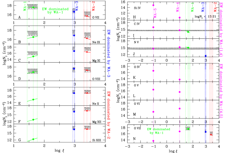
Figure 14: The column densities of the various X-ray (panels A-G on the left and N on the right) and UV (panels H-J on the right) found in the high resolution spectra of IRAS 13349. Panels K-M, on the right, give the column densities for some of the intermediate theory predicted ions, barely detected in the X-rays. The horizontal hashed regions in the left panels A to G, correspond to derived $N_{\rm j}\;$based on fits to the line series (see Table 3 and Section 3.1), but weighted according to the amount that the X-ray warm absorbers 1 to 3 contributes to it. Respectively, from left to right, green, blue and red points correspond to the best fit $N_{\rm j}\;$as determined by xstar fits for absorbers WA-1, WA-3, WA-2. It can be seen that OVII (panel A) is associated with WA-1, whereas ions in B–D and E–G panels correspond to WA-3 and WA-2 respectively. In the right panels I and J, the horizontal shaded strips represent the ionic column densities $N_{\rm j}\;$derived from the UV observations, assuming a Doppler parameter of $b=100$ ${\rm\thinspace km}{\rm\thinspace s}^{-1}\,$(Table 5). The right panels H–N have a different $\log\xi$ range, in order to accommodate WA-4 and WA-5 (marked with vertical dotted magenta lines).

4.3.2 UTA Contributions

As stated, our best model fit to the IRAS 13349 required a dust component for the X-ray fitting. For thoroughness, we investigate whether additional (gas phase) absorber components can take its place. In particular, L- to M-shell photoexcitations in lower charge states of Fe i to Fe xvi give rise to absorption at rest wavelengths 14 – 17.5 Å  ($\sim 0.7-0.89$ keV), $\sim$ the same spectral region where the dust absorption is required. These features, dubbed the Unresolved Transition Array or UTA (see Behar et al. 2001 and Gu 2007 for theory), was initially detected by Sako et al. (2001) based on an XMM RGS study of IRAS 13349. To test for the prevalence and strength of these lines based on our method of analysis (i.e. one which tie line strengths to the observed UV-Xray ionising SED), we explore fits which include additional absorber components that may account for them. (As a reminder, note that we began with an initial 9-absorber fit, covering the range $\rm-4\leq log\xi<4$, that would have accounted for all UTA lines, if significant.)

We begin by checking the range of ionization parameters where the ion fractions of Fe i to Fe xvi peak (middle panel of Figure 15). As can be seen in the figure, wa-(1-3) primarily account for the range of $\log\xi>1.49$, which while fitting for UTA ions Fe vii to Fe xvi, do not fully account for the Fe ii to Fe vi transitions that populate the spectral region between 17–17.5 Å  (0.71–0.73 keV rest; observed $\sim$ 18.8-19.4 Å=0.64–0.66 keV). Figure 15 shows that the “missing” low-ionization UTA lines should fall between $-3.0\leq\log\xi\leq 1.0$. As such, we include two additional warm absorber components: wa-4 (forced within $-1.0\leq\log\xi\leq 1.0$) and wa-5 (forced within $-3.0\leq\log\xi\leq-1.0$) to account for all “missing” UTA producing ions. The resultant fits (wa-4: $\rm log\,\xi\sim 0.99\;{with}\;\log N_{H}\sim-1.78$, and wa-5: $\rm log\xi\sim-1.02;{with}\;\log N_{H}\sim-1.86$) primarily affect O iv to O vi with the strongest contribution to O v (24.8 Å  observed) and O iv (25.2 Å  observed) absorption, while the fit statistics ($\Delta C=1.138;\,\chi_{\nu}^{2}=1.099)$ are still poorer than our best fit 4WA+dust fit, although marginally. (See Section 4.3.3 for details on fitting for dust in X-ray spectra.) Indeed, as can be seen in Figures 14 and 15, wa-4 contributes noticeably to the column density for these lower ionization oxygen (K–M) and UV ions (H–J), while wa-5 give $N_{\rm j}\;$values which are higher than those constrained by our HST measurements of Si iv and C iv. Nevertheless, this argues strongly for the UV and low-$\xi$ X-ray warm absorbers 3-5 having similar origins, as also borne out based on kinematics (see Section 4.3.4). (For subsequent fits, we exclude wa-5 because it does not obviously contribute to the fits in a positive way.) It can be seen from Figure 16 (blue) that the UTA alone cannot account for all the absorption in this spectral region.

4.3.3 Direct X-ray detections of iron dust

As just described, the UTA, while present, is unable to account for all absorption in the 17–17.5 Å  (0.71–0.73 keV rest; observed $\sim$ 18.8-19.4 Å = 0.64–0.66) spectral region. It was initially proposed by Lee et al. (2001), based on a Chandra HETGS study of the Seyfert galaxy MCG -6-30-15, that dust can be directly detected in high resolution spectra of X-ray bright objects. For iron-based dust, these features appear in the form of Fe L (iii, ii, i) photoelectric edges between (lab) $\sim 14.7-17.5$ Å  (0.7-0.84 keV; overlapping with the UTA spectral region). (Fe-based dust in astrophysical environments can also be measured at $\sim$ 7 keV Fe K – see Lee & Ravel 2005, but this is not relevant to the Chandra HETGS capabilities.) As can be seen in Figure 16 (blue), the UTA is unable to account for much of the absorption between 19.3-19.5 Å  (observed; $\sim 0.63-0.64$ keV), consistent with the Fe L iii edge (redshifted to $z_{\small{IR13349}}$) - in the context of IRAS 13349, this argues strongly for direct detections of iron-based dust in the AGN environment.

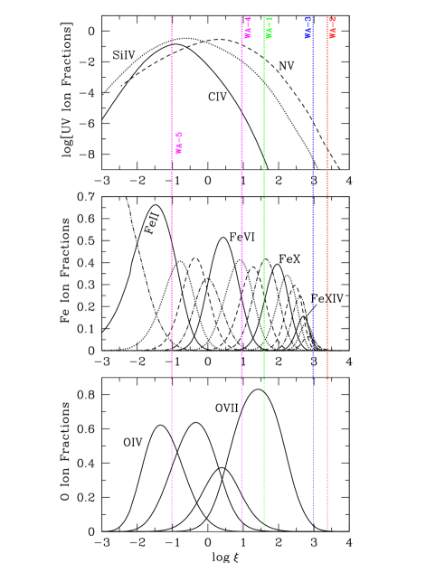
Figure 15: The distribution of ion fractions for the Fe i–Fe xvi ions (middle panel), responsible for the UTA, as a function of the ionization parameter. For comparison, we also plot the ion fraction distributions of some of the relevant, prominent UV (top panel) and X-ray ions (O IV–VII, bottom panel). Vertical dotted lines mark the best fit $\xi$ values of the various warm absorber components (see Section 4.3.2 for details).

To investigate the direct detection of iron-based dust in IRAS 13349, we incorporate cross sections associated with condensed matter forms of iron into our 4-absorber fit to determine an ionic column for iron in grains to be $N_{\rm Fedust}\sim(1.2\pm 0.21)\times 10^{17}\,\hbox{${\rm\thinspace cm}^{-2}\,$}$. (See Lee et al. 2009 for details on X-ray methodology for determining the quantity and composition of interstellar dust.) Using the ISM abundance values of Wilms et al. (2000), this translates to an equivalent Hydrogen column $N_{\rm H}\sim(4.5\pm 1.30)\times 10^{21}\,\rm cm^{-2}$. While the X-ray data are not of sufficient S/N to distinguish the exact iron composition (e.g. pure Fe vs. FeO vs. $\rm Fe_{2}O_{3}$ vs. $\rm Fe_{2}O_{4}$), a conservative estimate of an observable transmission signal, requires that the iron-based grains have thickness $\rm t\sim 0.1-0.8~{}\mu m$, based on the formalism for transmission $T=e^{-\mu\rho t}$, where $\rho$ is the density of the specific compound as defined from “The Handbook of Chemistry and Physics”; the values for the attenuation length were obtained from the CXRO at LBL, and NIST. Furthermore, the fits strongly suggest that at least 90% of the Fe is locked up in grains, with a minor contribution from gas phase iron, $N_{\rm Fe-gas}\sim 2.1\times 10^{15}\,\hbox{${\rm\thinspace cm}^{-2}\,$}$.

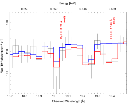
Figure 16: The Chandra MEG observed spectrum zoomed into the UTA and iron dust spectral region, at the redshift of IRAS 13349 (black). It is clear that ionised gas alone (5-warm absorbers including the UTA) is unable to explain all the absorption in this region (blue; see Section 4.3.2 for detailed discussion on UTA), and additional absorption with origins in iron-dust in IRAS 13349 is also needed (red; Section 4.3.3).

4.3.4 The absorber kinematics

Of interest, the outflow velocities for the X-ray absorbers we detect are best matched to the higher velocity ($\sim 950$${\rm\thinspace km}{\rm\thinspace s}^{-1}\,$) UV outflowing component. –See e.g. Figure 17 comparison of the HETGS view of O vii versus STIS view of N v. Figure 14 shows that the observed column densities for the UV ions C iv and N v (panels I and J) are consistent, within errors, with the xstar predicted column densities for the low $\xi$ phase of the warm absorber, determined from fitting to the Chandra spectra (OVII, panel N). Our analysis shows that the low-$\xi$ (WA-1 and WA-4) can have linked UV and X-ray absorption from C iv to O vii and some O viii, although the latter is primarily associated with the higher-$\xi$ WA-2 and WA-3.

Figure 17: A velocity profile comparison of the X-ray and UV absorbers, based on representative ions show that the UV and low-$\xi$ X-ray warm absorbers likely have a common origin. (TOP): velocity spectrum combined from the five strongest (X-ray) resonance lines of O vii based on Chandra MEG X-ray spectra, and (BOTTOM) velocity spectrum combined from two strong N v absorption lines seen in HST STIS spectra. Details for how these are generated can be found in Section 3.1.

Furthermore, it would appear that the lower ionisation phases are associated with a higher outflowing velocity. Our lower limits on the derived values for $v_{\rm blue}$ are roughly consistent with the upper limit findings by Sako et al., (2001; $v_{\rm blue}=420_{-180}^{+190}$ ${\rm\thinspace km}{\rm\thinspace s}^{-1}\,$) and Holczer et al. (2007; $v_{\rm blue}=300\pm 50$ ${\rm\thinspace km}{\rm\thinspace s}^{-1}\,$) if we account for the difference in choice of redshift value, i.e. $z=0.10764$ (Kim et al., 1995) used by previous authors versus the $z=0.108530$ value derived in this paper based on higher resolution HET data. We do not find any evidence for the $\sim+20$ ${\rm\thinspace km}{\rm\thinspace s}^{-1}\,$outflow reported by Sako et al. however, and our fitted turbulent velocity widths are slightly lower than the $v_{\rm turb}\sim 640$ ${\rm\thinspace km}{\rm\thinspace s}^{-1}\,$values reported by both Sako et al., and Holczer et al.

5 Discussion

5.1 Thermodynamics and structure of absorber

A topic of active debate is whether warm absorbers in AGN are in a continuous medium or are an ensemble of discrete clumpy media which are in different thermodynamic phases in near pressure equilibrium with each other. The answer to this question has interesting consequences for the geometry of the AGN environment, as a whole. Here, we use stability curves to demonstrate that the choice of ionising SED (e.g. X-ray versus the full source SED) for IRAS 13349 is very relevant in the conclusion for one scenario over the other.

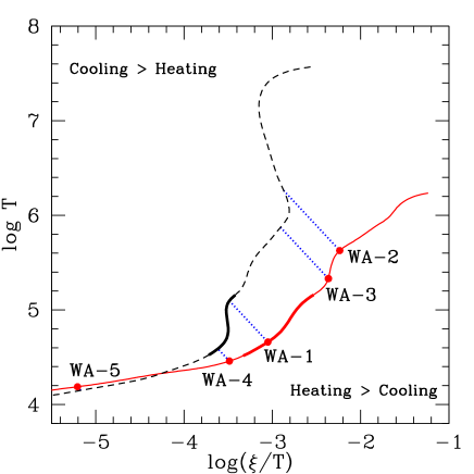
Figure 18: Stability curves illustrating differences in the thermodynamic behaviour of the absorbing gas as illuminated by the full UV–X-ray SED (solid red curve corresponding to the SED in solid red shown in Figure 10, bottom panel), versus an X-ray only ionising SED (black dashed curve corresponding to same representation of ionising SED in Figure 10, bottom panel). The unstable regions identified by the Holczer et al. (2007) analysis of this Chandra X-ray data based on an X-ray only ionising SED is highlighted in bold black. Also in bold on the red curve is the aforementioned unstable region translated over the same $\Delta T$ for the stability curve drawn based on a UV (i.e. accretion disc) inclusive SED. The filled circles on the red curve are the points corresponding to WA-1, WA-2, WA-3, WA-4 and WA-5 as predicted by the xstar fits to the Chandra HETGS data and the HST STIS data and/or theoretical considerations, as discussed in Section 4.3. As can be seen, no unstable regions are identified by our analysis. The dotted blue lines connect the points with the same $\xi$ values in the two curves, thus showing that the temperature for all the $\xi$ values are higher for the gas ionised by the X-ray only SED, except for WA-5, where the temperatures are equal.

Stability curves are thermodynamic phase diagrams of temperature ($\log T$) versus pressure ($\log(\xi/T)$, where $\xi\equiv$ ionisation parameter. It is an effective theoretical tool often used to discuss the thermodynamics of photoionized gas associated with the X-ray and UV absorbers (e.g. Krolik et al., 1981; Krolik & Kriss, 2001; Reynolds & Fabian, 1995; Chakravorty et al., 2009, and the references therein). By definition, an isobaric perturbation of a system in equilibrium is represented by a small vertical displacement from the stability curve; such perturbations leave $\xi/T\sim L/pR^{2}$ constant, which for constant $L/R^{2}$ leave the pressure unchanged. Any ‘system’ located on the part of the curve with positive slope is a stable thermodynamic system, because a perturbation corresponding to an increase in temperature leads to cooling, while a decrease in temperature leads to heating of the gas. If the stability curve is characterised with discrete allowed values of temperature at the same pressure, it points to a cloud-like absorber, whereas a wind-like scenario will have a continuous distribution of allowed temperature and pressure. Before proceeding, it is informative to briefly discuss the definition of the ionisation parameter in the context of stability curves. In the definition $\xi\sim L/nR^{2}$, it is conventional to use the luminosity $L$ in the energy range $13.6\,{\rm eV}-13.6\,{\rm keV}$ (i.e $1-10^{3}$ Rydberg). The warm absorber properties are, however, determined by the photon distribution in the soft X-rays ($E\gtrsim 100\,{\rm eV}$) and not by photons with energy $E<<100\,{\rm eV}$. Hence, in the making of warm absorber stability curves, authors often use modifications in the definition of the ionisation parameter. For example, Chelouche & Netzer (2005, and references therein) use an ionisation parameter $U_{x}$ which considers the ionising flux only between $540\,{\rm eV}\,\,\rm{to}\,\,10\,{\rm keV}$. Chakravorty et al. (2012), on the other hand, simply normalise the stability curves by using the ratio of the total luminosity to the luminosity in the X-ray power-law component in the SED. However, it is to be noted that these modifications simply shift the entire stability curve along the $\log(\xi/T)$ axis and does not change the nature of the kinks or curves in the stability curve. For example, the range ($\Delta[\log(\xi/T)]$ or $\Delta T$) of the stable or unstable regions of the stability curves would remain unchanged with such modifications of the ionisation parameters. As such, all the qualitative properties of the stability curves and comparisons between the stability curves of different SEDs, discussed subsequently, would remain the same even if better definitions of the ionisation parameter are used.

In the context of AGN warm absorbers, several authors (e.g. Krolik et al., 1981; Krolik & Kriss, 2001; Gehrels & Williams, 1993) have commented that the gas in the $4.5<\log T<5$ region is thermally unstable, since the cooling function $\Lambda(T)$ has a negative gradient in this temperature range. As such, the ions detected on the stable regions of the stability curve bracketing this temperature range would be attributed to cloud-like absorbers where the different phases are in pressure equilibrium with each other. Based on the findings for just such an ionisation gap in IRAS 13349 by Holczer et al. (2007) using data from the Chandra HETGS (the same data we are re-analysing in this paper) and Sako et al. (2001) with the XMM-Newton RGS, cloud-like clumpy absorbers would appear to be the conclusion one would draw for this quasar. (We note however that Sako et al. 2001 acknowledge that their stability curves do not show thermodynamically unstable regions for IRAS 13349.) In a comparison with the Holczer et al. (2007) results, the fact that their absorption measure distribution (AMD) methodology, despite assuming a continuous distribution of ions at the onset, concludes for thermodynamically unstable regions, further strenghtens the case that independent of fitting technique (AMD vs. photoionisation modelling as that employed here e.g.), it is the ionising SED that is the critical factor.

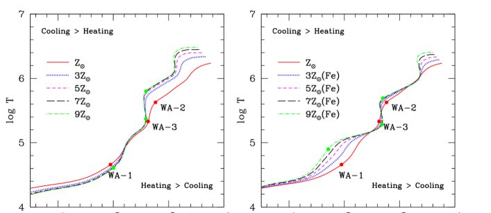
Figure 19: Stability curves corresponding to super-Solar gas of $3Z_{\odot}(\rm blue),5Z_{\odot}(pink),7Z_{\odot}(black),{\rm and}\,\,9Z_{\odot}({\rm green})$, where (LEFT) $Z_{\odot}$ refers to all Z-elements, and (RIGHT) $Z_{\odot}$ refers only to iron, i.e. only iron abundance are altered here. For comparison, in both panels, solar abundance stability curves are shown in solid red, and plotted points correspond to xstar predicted ionisation phases for the warm absorber.

Reynolds & Fabian (1995) and Chakravorty et al. (2012) discuss and demonstrate that a moderate to strong soft excess component makes the stability curve more stable at $10^{5}$ K (see also Krolik et al., 1981). Chakravorty et al. (2012) further demonstrate in general for AGN that the inclusion of the accretion disc spectral component in the EUV range in addition to a significantly strong soft excess may completely remove the apparent thermal instability in the aforementioned temperature range. In this paper, we revisit the conclusions for the thermodynamic stability conditions for the IRAS 13349 warm absorber gas in the context of different SEDs: one that excludes the disc components (aforementioned X-ray studies of IRAS 13349), and one which includes them (this paper). For our simulations of the photoionized gas thermodynamic properties, we used xstar to model a spherical shell of solar metallicity gas having $N_{\rm{H}}=5\times 10^{21}\,\rm{cm^{-2}}$ and particle density $n_{\rm{H}}=10^{9}~{}\rm{cm^{-3}}$, illuminated by the aforementioned SEDs. It should be noted that the stability curves are insensitive to the choice of $10^{3}\leq n\leq 10^{12}\rm cm^{-3}$ for the IRAS 13349 ionising spectra. It can be seen from Figure 18 that the choice of ionising spectrum strongly influences the conclusions for gas thermodynamic stability. For the two curves shown, we use thicker lines to highlight the temperature range conventionally established to be unstable (negative slope) for photoionized gas in AGN environments. It can be seen that an X-ray only (disc-free) ionising SED leads to the prediction (black dashed curve) for a narrow range of $\xi$ coincident with the aforementioned temperature range over which the warm absorber is mildly unstable. Indeed, it is exactly the finding for ions on either side of this unstable phase seen in the black dashed curve that led Holczer et al. (2007) to their conclusions for IRAS 13349. In contrast, when we include the UV as part of the ionising input, no such instability is seen, thereby pointing to a flow that is more wind-like and continuous in IRAS 13349. The effect of the excess UV photons due to the addition of the accretion disk component, facilitates the formation of OVII and other ions with similar ionization potential (see panel D of Figure 12). OVII acts as a cooling agent and hence lowers the temperature of the gas, which results in thermodynamic stability in the region of WA-1. Moreover, the accretion disk component also helps to lower the Compton temperature of the gas. Hence the temperature of the curve in the region of WA-3 is lowered, rendering this part of the curve stable, as well. Thus, while our analysis reveals similar ionisation states found from previous studies, the additional consideration of the UV-influence drives us to a conclusion that the ionised absorber in IRAS 13349 should be more continuous and wind-like than discrete clouds.

Taking the thermodynamic instability-free red curve in Figure 18, it is interesting to further consider the conditions driving the fit results. Specifically, as discussed in Section 4.3, the components WA-1 and WA-2 are statistically ‘sufficient’ to fit the Chandra HETGS data. However there are no thermodynamically unstable phases between these two points to separate them — as seen in the figure (red curve). In other words, there is a range of $\xi$ which is theoretically allowed by thermodynamic calculations and yet is not required while fitting the data. While one explanation for this may be the insufficient S/N of the available data, there may be additional more physically motivated answers. Specifically, (1) there may be an absence of absorbing material of sufficient column density at certain intermediate ionisations (which may be related to intermediate distances from the black hole) to imprint significantly on our spectrum. Indeed, for IRAS 13349, when we ‘force fit’ a third component WA-3 to the data, its physical conditions ($\xi$, $\rm{N_{H}}$ and $\rm{v_{blue}}$) come out to be intermediate between that of WA-1 and WA-2. Further, (2) when we include additional theoretically motivated component WA-4 and WA-5 to account for the entire UTA, we indeed populate the entire stability curve suggesting presence of material in a continuous distribution of ionisation states The stability conditions of a super-solar warm absorber would be distinctly different from that of a gas with Solar abundances (see Chakravorty et al., 2009, 2012). Since the outflowing gas from the nuclear regions of AGN may indeed have super-solar metallicities (e.g., Arav et al. 2007), we explore this idea further for IRAS 13349 in the next section.

5.1.1 Super-solar metallicities

Chakravorty et al. (2009, 2012) show that the stability curves for a super-solar absorber is more likely to show discretely separated multi-phase structure. In Figure 19 we show the stability curves for different super-solar metallicites of the absorber. Independent of whether only iron, or all metals are varied, it can be seen that the higher metallicity gas starts exhibiting thermodynamic instability at $\log T>5.2$, and the high ionisation phase WA-2 ($\rm log\,\xi\sim 3.4$; top-most, green circle) falls in a part of the curve after it recovers from this instability. However, there is no distinct unstable region between the low WA-1 ($\rm log\,\xi\sim 1.7$) and intermediate WA-3 ($\rm log\,\xi\sim 3$) ionisation phases which would mean a continuous distribution of phases in this range of ionisation parameters. WA-3 falls exactly at the turnover where the high metallicity curves become unstable at $\log T>5.2$, suggesting that while WA-2 and WA-3 are thermodynamically separated, they are nevertheless in pressure equilibrium. It is of further interest to note that the WA-2 and WA-3 values derived from xstar fits to the Chandra data fall on opposite ends of the unstable regions in Figure 19.–This may not be coincidental, since gas in the unstable regions would preferentially migrate towards stable region, by cooling or heating. Ultimately, if there are discrete (rather than continuous) absorbers in IRAS 13349, at least some components of the gas must have super-solar metallicities.

We would like to caution that our discussion of super-solar metallicities is not quantitatively absolute and should only be considered as a qualitative impression of our expectations. A more rigorous study would involve fitting the data with super-solar population files in xstar and drawing conclusions based on the best-fit metallicity of the absorber. Given the S/N of our data, however, such detailed fits are not warranted in this paper.

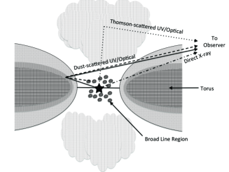
Figure 20: Inferred geometry of IRAS 13349. See §5.2 for details.

5.2 The IRAS 13349 dusty warm absorber

Given the Reynolds (1997) finding back in the ASCA era that $\sim 20$% of the warm absorber Seyfert 1s have significant optical reddening, it is not surprising that there is now a remarkable convergence of evidence for dusty ionised winds from observations with more powerful satellites. That IRAS 13349 harbours dust has long been established with IR (Beichman et al. 1986; Barvainis 1987), UV/optical (Wills et al., 1992; Hines et al., 2001) and X-ray (Brandt et al., 1996, 1997) studies. Using the superb multi-wavelength data set presented here, in combination with knowledge based on prior work, we present a geometrical model for the IRAS 13349 line-of-sight (LOS), and location of dust, based on dust modelling of the absorbed optical-UV spectra (Section 5.2.2) , and direct IR and X-ray measurements (Section 5.2.3) of dust properties.

5.2.1 A model for the IRAS 13349 dust

As we showed in §4.1, the direct UV and optical flux from IRAS 13349 is substantially lower than would be expected for a typical QSO. Additionally, the high polarisation rising to shorter wavelengths (Hines et al., 2001) is indicative of scattering by dust. Hines et al. (2001) attempted to model the UV/optical flux and polarisation of IRAS 13349 as a combination of a direct view of the nucleus reddened by an intervening screen, plus dust-scattered light from biconical regions filling the poles above the obscuring torus. Using dust with SMC-like properties, they were able to obtain a reasonable match to the shape of the polarised flux spectrum, but the predicted total flux spectrum did not match the observations—the optical flux was much too high, and the reddening caused the predicted UV flux to drop far below the observed intensity. When one also considers the shorter-wavelength data from STIS presented in this paper, the fact that the UV flux is much higher than predicted by their model suggests that there could be additional scattering that is colour neutral, e.g., like the Thomson mirror of hot electrons in NGC 1068 (Antonucci & Miller, 1985). This idea is reminiscent of the original suggestion by Wills et al. (1992) that the polarised light in IRAS 13349 was due to Thomson scattering, although that idea proved inconsistent with the wavelength dependence into the near-UV observed by Hines et al. (2001). For our proposed geometry here, the Thomson-scattered component would play a minor role in the polarisation, and only account for the flux at the shortest wavelengths.

To test this idea, we developed a simple heuristic model as illustrated in Fig. 20. As shown in the figure, our direct line of sight (the dash-dot line) to the active nucleus passes through the upper atmosphere of the obscuring torus. The atmosphere consists of a mixture of highly ionised gas and dust that has not yet been evaporated by the incident radiation. This line of sight is heavily reddened in the UV/optical band, or even completely blocked; in the X-ray, since the gas is highly ionised, there is little absorption by lighter elements, and the active nucleus is visible (Brandt et al., 1997). A second line of sight (the solid line and the dashed line) passes through less dense portions of the atmosphere that are more transparent at UV/optical wavelengths, but this line of sight only gives a view of the active nucleus as reflected by dust from the far wall of the obscuring torus. Finally, a third line of sight passes above the atmosphere of the torus, and it has a view of the nucleus that is Thomson scattered from hot electrons in the thermal wind escaping along the polar cavities of the torus.

Assuming the active nucleus plus BLR has a spectrum identical to the composite QSO spectrum (defined as $f_{\rm c}$), this model can be analytically expressed as:

$$F_{\rm optUV}(\lambda)=\left[F_{\rm direct}(\lambda)+F_{\rm scat}(\lambda)+F_{\rm Th}(\lambda)\right]\times 10^{-0.4A_{\rm V}g(\lambda)}$$ (5)

where $A_{\rm V}$ is the optical absorption within our Galaxy and $g(\lambda)\,=\,A_{\lambda}/A_{\rm V}$ is the extinction law in the Milky Way, as defined in Fitzpatrick (1999). The other components within the IRAS 13349 galaxy are:

$\bullet$ Absorbed direct flux in the torus, torus atmosphere, and galaxy: We define the LOS flux passing directly through the torus by:

$$F_{\rm direct}(\lambda)=\Gamma_{\rm d}\,f_{\rm c}(\lambda)$$

$$\times 10^{-0.4\ (A_{{\rm V}_{\rm{tor}}}\,g_{\rm{tor}}(\lambda)+A_{{\rm V}_{\rm{atm}}}\,g_{\rm{atm}}(\lambda)+A_{{\rm V}_{\rm{gal}}}\,g_{\rm{gal}}(\lambda))}$$

where $\Gamma_{\rm d}$ is the absolute normalisation of the composite spectrum, $A_{{\rm V}_{\rm{tor}}}$ and $g_{\rm tor}(\lambda)\,=\,A_{\lambda_{\rm{tor}}}/A_{\rm V_{\rm tor}}$ are the optical absorption and the wavelength-dependent extinction law within the torus, $A_{\rm V_{\rm atm}}$ and $g_{\rm atm}(\lambda)\,=\,A_{\lambda_{\rm atm}}/A_{\rm V_{\rm atm}}$ are the optical absorption and the wavelength-dependent extinction law within the torus atmosphere, and $A_{\rm V_{\rm{gal}}}$ and $g_{\rm gal}(\lambda)\,=\,A_{\lambda_{\rm gal}}/A_{\rm V_{\rm gal}}$ are the optical absorption and the wavelength-dependent extinction law within the galaxy, respectively.

$\bullet$ Absorbed dust-scattered UV/optical flux in the torus atmosphere and diffuse medium:

$$F_{\rm scat}(\lambda)=\gamma_{\rm scat}\,\Gamma_{\rm d}\,f_{\rm c}(\lambda)\left(1+\frac{\lambda}{\lambda_{\rm c}}\right)^{-\alpha}$$

$$\times 10^{-0.4\ (A_{\rm V_{\rm{atm}}}\,g_{\rm{atm}}(\lambda)+A_{{\rm V}_{\rm{gal}}}\,g_{\rm{gal}}(\lambda))}$$

where $\left(1+\frac{\lambda}{\lambda_{\rm c}}\right)^{-\alpha}$ stems from the wavelength dependence of the scattering ($\alpha=4$ is the Rayleigh limit), $\lambda_{\rm c}$ is the critical wavelength of the scattering, characteristics of the typical dust grain size, and $\gamma_{\rm scat}$ is the fraction of direct light which is dust-scattered.

$\bullet$ Absorbed Thomson-scattered UV/optical flux in the diffuse medium:

$$F_{\rm Th}=\gamma_{\rm{Th}}\,\Gamma_{\rm d}\,f_{\rm c}(\lambda)\times 10^{-0.4\ A_{\rm V_{\rm{gal}}}\,g_{\rm{gal}}(\lambda)}$$ (8)

where $\gamma_{\rm{Th}}$ is the fraction of direct light which is Thomson scattered.

5.2.2 The wavelength-dependent extinction within IRAS 13349

With this model in mind, we consider, through $\chi^{2}$ fitting, which combination of dust absorption and scattering best-describes the IRAS 13349 observed optical-UV spectrum. We used the Levenberg-Marquardt minimisation to determine goodness of fit, based on the IDL code mpfit (Markwardt, 2009). However, we do not have any information about the extinction within IRAS 13349, neither in the galaxy nor in the torus and torus atmosphere. We therefore considered several permutations of existing laws previously published for the MW (Fitzpatrick, 1999), the average SMC and LMC (Gordon et al., 2003), and starburst galaxies (Calzetti et al., 2000). The worst fits were obtained with the MW and/or LMC extinction, due to the presence of the $2175$ Å bump in these laws. This points towards IRAS 13349 lacking the unknown dust population responsible for this $2175$ Å absorption feature in the MW and the LMC, in good agreement with several studies showing that the dust content in AGNs is SMC-like (see e.g. Crenshaw et al., 2001; Hopkins, 2004, and references therein). As expected, the use of the SMC and/or the Calzetti laws gives better results, but the fits are still poor, with reduced $\chi^{2}\,\geq\,3$.

We therefore build our own SMC-like extinction laws for the IRAS 13349 torus, torus atmosphere, and galaxy as:

$$g_{\rm tor}(\lambda)\,=\,\left(\frac{5448~{}\textrm{\AA}}{\lambda}\right)^{\beta_{\rm tor}}$$ (9)

in the torus,

$$g_{\rm atm}(\lambda)\,=\,\left(\frac{5448~{}\textrm{\AA}}{\lambda}\right)^{\beta_{\rm atm}}$$ (10)

in the torus atmosphere,

$$g_{\rm gal}(\lambda)\,=\,\left(\frac{5448~{}\textrm{\AA}}{\lambda}\right)^{\beta_{\rm gal}}$$ (11)

in the galaxy. These laws are built so that they are equal to 1 in the $V$ band, and we assume the dust population is different in the torus, the torus atmosphere and the rest of the galaxy. In our fit, the spectral indices $\beta_{\rm tor}$, $\beta_{\rm atm}$, and $\beta_{\rm gal}$ are free parameters along with the optical extinction within the torus $A_{\rm V_{\rm tor}}$, the atmosphere $A_{\rm V_{\rm atm}}$, and the galaxy $A_{\rm V_{\rm gal}}$, the fraction of dust- and Thomson-scattered light $\gamma_{\rm scat}$, $\gamma_{\rm Th}$, and the critical dust-scattering wavelength $\lambda_{\rm c}$. The absolute normalisation of the composite spectrum $\Gamma_{\rm d}$ is fixed to the level discussed in Section 4.1, the dust-scattering spectral index $\alpha$ is fixed to 4 (Rayleigh limit), and the optical extinction within the MW is fixed to $A_{\rm V_{Gal}}=0.04$ ala the Wills et al. (1992) derived value for IRAS 13349.

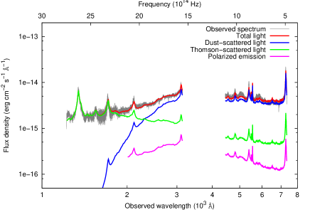
Figure 21: Best-fit model for the UV/Optical spectrum of IRAS 13349 (observed spectrum in grey). The full modelled spectrum is the red line. The Thomson-scattered component is the green line, and the dust-scattered component is the blue line. We also include the polarised light (magenta) as measured in Hines et al. (2001). Our fit results point to the direct light having marginal contribution, pointing to almost complete obscuration by the torus in the UV and optical.

$\bullet$ Best-fit dust model:    In our fitting, we are unable to constrain the fraction of dust-scattered light $\gamma_{\rm scat}$ as it systematically pegs to 1. We can interpret this as due to (1) an overestimation, by the composite spectrum, of the nucleus continuum in the optical or, (2) the presence of another contributing component in the optical domain. We therefore fix $\gamma_{\rm scat}=0.2$, a conservative value chosen to reflect the absolute normalisation of the absorbed UV spectrum needed to bring IRAS 13349 in line with unabsorbed QSO behaviour (see Section 4.1 for details). Likewise, it appears difficult to constrain any torus parameters, since all fits tends towards removing the direct light. This strongly suggests that the direct light is completely blocked by the torus, and so we fit using only the dust- and Thomson-scattered light. Our best fit (Figure 21 and Table 9) points towards a steep extinction law within the torus atmosphere ($\beta_{\rm{atm}}\sim 3.01$), while the extinction within the galaxy is flatter, with $\beta_{\rm{gal}}\sim$2.11, but steeper than that of the SMC. The typical grain size derived from the dust-scattering function $a\approx\lambda_{\rm c}/2\pi\sim 1.21$ $\mu$m, is consistent with large grains within the torus atmosphere absorbing the dust-scattered light in the far-UV, where the emission is dominated by Thomson-scattering, with $\gamma_{\rm Th}\sim 2.4$%. We have checked that the lower normalisation for the UV peak ($\sim$factor-of-two compared with the Elvis 1994 value we use; see Section 4.1 for details) predicted by the Hopkins et al. (2007) SED give roughly similar dust fit results.

We attempted to, but ultimately could not include polarisation in any reasonable way in these fits to garner believable measurements, although the conclusions based on our polarisation-free fits are consistent with those of Hines et al. (2001) based on polarisation studies. Specifically, Hines et al. showed that polarisation is wavelength-dependent, therefore pointing to dust-scattering dominating over wavelength-independent Thomson-scattering. Similarly, our fits point strongly to dust-scattered light dominating the 2000 and 8000 Å  spectral region.

5.2.3 Direct X-ray and IR measurements of the IRAS 13349 dust

Using additional knowledge gained from direct X-ray and IR measurements of the IRAS 13349 dust properties as enabled by the superb spectral resolution of the Chandra HETGS and Spitzer IRS, we further consider the location of the different composition grains we detect.

$\bullet$ Chandra X-ray spectroscopic detection of iron grains:

As described in Section 4.3.3, we directly detect iron-based dust in the X-ray corresponding to $N_{\rm H_{FeGrains}}=(4.5\pm 1.30)\times 10^{21}\,\rm cm^{-2}$ and grain size $\sim 0.1-0.8$ $\mu{\rm m}\;$. According to the radiative transfer calculations of Kama et al. (2009), iron sublimates between $\sim$ 1000–2700K as a strong function of densities (i.e. pressures). The protoplanetary disk conditions that they consider has typical vapour densities of $\sim 10^{-12}$–$10^{-10}\rm g\,cm^{-3}$ which translates to particle density $\sim 10^{10}$–$10^{12}\rm atoms\,cm^{-3}$, assuming 55  $\rm grams\;moleFe^{-1}$, not dissimilar to the particle densities that one would expect for the inner AGN clouds. More importantly, at these densities, iron sublimates at 1400K, a higher temperature than silicates at 1100-1300K. As such, in the context of our geometrical model for the IRAS 13349 viewing geometry (Figure 20), we can place the iron in the upper, less optically thick layers of the torus atmosphere, with the silicates more towards the interior. Furthermore, in adopting the formalism

$$R_{d}\simeq 0.4\,\left(\frac{L}{10^{45}\rm erg\,s^{-1}}\right)^{1/2}\left(\frac{1500K}{T_{\rm sub}}\right)^{2.6}\rm pc$$ (12)

derived by Nenkova et al. (2008), we find $\sim 2.7-5.2$ pc for the inner radius of cloud distributions in a clumpy torus for sublimation temperatures T$\sim 1100-1400$K and $L_{\rm bol}\sim 3\times 10^{46}\rm\hbox{${\rm\thinspace erg}{\rm\thinspace s}^{-1}\,$}$ (see Table 7). The Keck Interferometer measurements of Kishimoto et al. (2009) point to dust at $\sim 0.92$ pc, which suggests either dust T $\sim$ 2000K or larger dust grains (e.g. 1.2$\mu{\rm m}\;$  as derived based on spectral fitting in Section 5.2.1) – see also (Sitko et al., 1993, e.g.).

$\bullet$ Spitzer IRS spectroscopic detection of silicates and PAHs

As discussed in Section 3.4, the Spitzer IRS spectra show weak 7.7 $\mu{\rm m}\;$and 11.3 $\mu{\rm m}\;$PAH, as well as broad 10 $\mu{\rm m}\;$and 18 $\mu{\rm m}\;$silicate emission. The PAHs are associated with the outer starbursting part of the galaxy and therefore play no role in the dust absorption and scattering effect considered previously. Even if the obscuration is a supernova heated starburst disk (see e.g. theory in Fabian et al. 1998; Wada & Norman 2002; Thompson et al. 2005; Ballantyne 2008), in the IRAS 13349 host galaxy, any PAHs will have to be far enough away from the strong radiation to have little effect. Else, for the detected silicates, given that they are in emission, just like in other normal quasars and Seyfert 1s, it is quite clear that we are not looking through a lot of dust, but rather are at a high-enough elevation angle above the torus to clear the densest gas, but perhaps just grazing the surface and looking through its atmosphere, which is what is causing the UV and X-ray absorption lines and the extinction of the UV continuum.

Furthermore, the 10$\mu$m peak is shifted to the red, indicating either a depletion of small dust grains or more crystalline silicate dust (e.g. enstatite) rather than amorphous olivine. The opacity at the 1.844 keV (6.724 Å, rest) Si K edge is too low for us to verify the type of silicates with X-ray data. However, the fact that the dust we do detect in the X-rays is primarily locked up in iron, argues strongly for the silicates to be Mg-rich (e.g. forsterite). Markwick-Kemper et al. (2007) argue for forsterite in the PG 2112+059 BAL QSO wind based on Spitzer studies; one might imagine a similar dusty outflow for IRAS 13349, but as stated in Section 3.4.2, assessing the level forsterite may contribute to the 11.2 $\mu{\rm m}\;$ feature is beyond the scope of this paper.

In further estimating where the silicate dust responsible for the broad IR emission may reside, we derive $R_{\mathrm{sub}}\sim 1.2$ pc, using the relation $R_{\mathrm{sub}}=0.2(L_{\mathrm{bol}}/10^{46})^{1/2}$ pc (Laor, 1998, 2003). To arrive at this, we take the mid-IR luminosity of IRAS 13349 $\nu L_{\nu}(25\mu\mathrm{m})=3.2\times 10^{45}=L_{\mathrm{bol}}f_{\mathrm{c}}f_{\mathrm{i}}$ erg s^-1, where $f_{\mathrm{c}}\sim 0.6$ is a representative dust covering fraction and $f_{\mathrm{i}}\sim 0.5$ is a representative mid-IR anisotropy for quasars (Ogle et al., 2006; Shi et al., 2005). Based on this, it is likely then that the dust responsible for the mid-IR continuum is the same dust that absorbs the direct optical-UV spectrum, since it accounts for a large fraction of the absorbed and reprocessed bolometric luminosity of the quasar.

5.3 The dusty wind in IRAS 13349: torus or accretion disk origin?

Given the excellent qualitative agreement between our proposed model for the dust contributions (Section 5.2.2) and the observed spectrum, our picture in Figure 20 must be close to reality. One additional piece of evidence in support of our model can be gleaned from the existing polarisation data. Hines et al. (2001) note a difference in polarisation angle for the broad emission lines compared to the continuum. The line centres have their angles rotated by  5 deg, but the polarisation stays fairly constant. One can interpret this rotation in terms of the differing angle between the scattering region and the sources of the incident radiation, meaning that the BLR is displaced from the optical/UV continuum source by several degrees as viewed from the scatterer. Also, since the emission lines are not depolarised, the angles from across the full BLR to the scatterer must be within a fairly narrow range so that their polarisations do not cancel out. So, the size of the BLR as seen from the scatterer must be small. If we take the difference in polarisation angle as the offset of the BLR from the continuum source, then, given a distance for the BLR from the nucleus, we can deduce the distance of the scatterer from the continuum source. Scaling up reverberation mapping results for BLR sizes (Kaspi et al., 2005) to our extinction-corrected UV luminosity for IRAS 13349 ($\rm L_{1350}=7.95\times 10^{45}~{}\hbox{${\rm\thinspace erg}{\rm\thinspace s}^{-1}\,$}$), the BLR would be at a radius of $\rm r=7\times 10^{17}$ cm. The scatterer would then be at $8\times 10^{18}$ cm, or 2.6 pc, For comparison, the dust sublimation radius $R_{\mathrm{sub}}\sim 1.2$ pc we calculate in Section 5.2.3 (same value from Barvainis 1987), and the inner edge of the torus is expected to be at $\sim 1~{}\rm pc(L/10^{45})^{0.5}=2.8$ pc (Krolik & Begelman, 1988). This is remarkably consistent with the optical light being scattered light from the far wall of the torus. In adopting the classic picture presented whereby an obscuring torus is always present (Antonucci 1993; see also Lawrence & Elvis 1982) our view of IRAS 13349 then is at high inclination, barely skimming the surface of the torus.

This picture presents a problem then for scenarios of accretion-disk winds (e.g., Elvis 2000), where the wind streamlines favour the equatorial plane, parallel to the surface of the torus. Nevertheless, it is of interest to consider further an alternative to the torus for the obscuration, that would allow the wind to have an accretion disk origin. Recently, Czerny & Hryniewicz (2011) proposed a model for the creation of dusty winds at $\mathrel{\hbox to0.0pt{\lower 3.0pt\hbox{$\sim$}\hss}\raise 2.0pt\hbox{$>$}}1000R_{\rm S}$ by drawing parallels between clouds on quasar disk surfaces to similar temperature and pressure conditions that cause dust formation in AGB stars. In the context of the Elvis quasar model, the material in this wind would then be the cause of the obscuration, in lieu of the torus. But can this satisfy our condition for a high inclination viewing angle for IRAS 13349? Based on the wind flow lines shown in Fig. 3 of Risaliti & Elvis (2010), the scale height at which our line-of-sight intersects the dusty wind is $z=200R_{\rm S}=0.09$ pc at 1000$RR_{\rm S}^{-1}$ for a $10^{9}M_{\odot}$, quite close to the disk plane. Alternatively, a warped disk as the source of obscuration (Lawrence & Elvis, 2010), although for IRAS 13349, it would have to be contorted in such a way as to satisfy the known effects caused by dust scattering, absorption, and polarising. Else, if we again consider the putative torus, one might argue that our line of sight on the near side of the torus passes under the streamlines of the accretion disk wind, but then the line of sight from the nucleus to the far wall of the torus and back again must pass directly through the wind, and at multiple angles.

While the accretion disk wind idea is a desirable one, it is ultimately more difficult to reconcile, compared to a torus wind, for IRAS 143349. The line widths in our STIS spectrum are similar to the narrow, few hundred ${\rm\thinspace km}{\rm\thinspace s}^{-1}\,$ absorption lines common in other nearby AGN (Crenshaw et al., 2003; Kriss, 2002; Dunn et al., 2007), as expected for the thermal winds of Krolik & Kriss (1995, 2001). Also, the velocity shifts we detect in both UV and X-ray are slow compared to the ultra-fast outflows expected from the disk (Tombesi et al. 2010; see also Chartas et al. 2002; Pounds et al. 2003 for the first claims of such outflows in Seyferts).

If there is no disk wind in this object, then perhaps the conditions that drive it are just not right. The disk winds of Murray et al. (1995); Murray & Chiang (1995) require a high ionisation parameter and and a high column density at the inner edge of the wind, and IRAS 13349 does not have a high column density of either X-ray or UV-absorbing gas. The manifestation of a disk wind in an AGN may not be a universal property that depends only on orientation, but also on other intrinsic parameters such as the accretion rate or the Eddington ratio.

5.4 Similarities to non-black hole astrophysical systems

It is interesting that many apparent parallels can be drawn between IRAS 13349, a massive energetic black hole systems fuelling a whole galaxy, and other less powerful/smaller systems. For example, the relatively large grains found in the torus of IRAS 13349 are also encountered in the dusty winds of luminous blue variable (LBVs, see e.g. Robberto & Herbst, 1998; O’Hara et al., 2003). In these extreme massive stars, the maximum grain size is set proportionally to the mass-loss rate of the high-opacity wind, and dust is likely created during stellar eruptions, when this mass-loss reaches very high levels (0.001–0.01 $M_{\odot}$/yr, Kochanek, 2011). In IRAS 13349, the high-opacity component (characterised by the high optical extinction suffered by the direct light), and the dust appear to be co-located, suggesting perhaps also dust formation in the IRAS 13349 outflows, be it from the torus or disk. In addition, based on sublimation temperature arguments, our placement for the iron- grains (detected in the Chandra X-ray spectra) in the rim and upper layers of the torus with the silicates (detected in Spitzer IR data) in the interior, gives a picture qualitatively similar to that arrived at by Chiang et al. (2001) for the dust in the surface layers of T Tauri and Herbig Ae disks.

Parameters	Best-fit value	Definition
$\gamma_{\rm scat}$	0.2 (fixed)	Fraction of dust-scattered light
$\lambda_{\rm c}$ ($\mu$m)	$7.60\pm 0.62$	Dust-scattering critical wavelength
$\alpha$	4 (fixed)	Dust-scattering index
$A_{\rm V_{\rm atm}}$	$0.14\pm 0.02$	Optical extinction in atmosphere
$\beta_{\rm atm}$	$3.01\pm 0.08$	Spectral index of extinction in atmosphere
$\gamma_{\rm Th}$	$0.024\pm 0.003$	Fraction of Thomson-scattered light
$A_{\rm V_{\rm gal}}$	$0.05\pm 0.01$	Optical extinction in galaxy
$\beta_{\rm gal}$	$2.11\pm 0.11$	Spectral index of extinction in galaxy
$\chi_{\rm r}^{2}$ (d.o.f)	1.66 (862)

Table 9: Best-fit parameters. Uncertainties are given at the 2$\sigma$ confidence.

6 Summary

Although IRAS 13349 shows many signs of being an obscured QSO, the Spitzer spectra show it as a typical QSO. The continuum peaks at 30 $\mu$m; the silicate features at 10 and 18 $\mu$m are in emission, and PAH features are weak. The emission lines are dominated by highly ionised species such as $[$Ne v$]$ and $[$O iv$]$. Furthermore, even though IRAS 13349 exhibits extreme Eigenvector-1 characteristics, HET optical spectra argue against its classification as a narrow-line-Seyfert 1. The high signal-to-noise and $R\sim 1300$ HET data has also allowed us to improve redshift measurements for IRAS 13349, locating it at z=0.10853.

In the ultraviolet, our low-resolution STIS spectra cover the observed wavelength range from 1150–3180 Å. These spectra show for the first time blue-shifted absorption from Ly$\alpha$, N v and C iv, with components at systemic velocities of $-950~{}\hbox{${\rm\thinspace km}{\rm\thinspace s}^{-1}\,$}$ and $-75~{}\hbox{${\rm\thinspace km}{\rm\thinspace s}^{-1}\,$}$. The lines are unresolved, and they have intrinsic widths with Doppler parameters that are $<200~{}\rm\hbox{${\rm\thinspace km}{\rm\thinspace s}^{-1}\,$}$. As seen before (Hines et al. 2001), the UV spectrum is heavily reddened, but at the shortest wavelengths in the UV, below an observed wavelength of 1600 Å, the spectrum begins to recover in flux and appears less heavily reddened.

Our HETGS spectrum of IRAS 13349 covers X-ray wavelengths from 2–38 Å(observed). The continuum is well described by a power law with photon index $\Gamma=1.9$. At low energies we observe a soft X-ray excess that can be modelled as a black body with $kT\sim 100$ eV. IRAS 13349 is well known for the ionised absorption that is prominent in its X-ray spectrum (Brandt et al. 1996, 1997; Sako et al. 2001; Longinotti et al. 2003; Holczer et al. 2007). Our spectrum shows absorption lines attributable to at least two warm absorbers at velocities comparable to the higher velocity UV absorber. The lowest ionisation WA-1 is co-located with the UV absorber.

Using simultaneous Chandra HETGS and HST/STIS spectra obtained in February 2004, contemporaneous ground-based optical spectra from the HET, and archival Spitzer IRS spectra from 2005 as well as IRAS, ISO, and 2MASS photometry data, we have constructed a broad-band view of the SED of IRAS 13349. If we compare the observed SED of IRAS 13349 to the median QSO spectral energy distribution (SED) of Elvis et al. (1994), we see that the IR and X-ray bands are a good match, but the UV and optical are severely suppressed. This suggests that these portions of the spectrum are either heavily obscured and/or only viewed in scattered light. By normalising the peak of the infrared continuum and the absorption-corrected X-ray continuum to the Elvis et al. (1994) SED, we determine that the unreddened portion of the optical continuum represents a fraction of only 20% of the intrinsic light from IRAS 13349.

If we correct the observed SED of IRAS 13349 for scattering and extinction, it peaks at a rest wavelength of $\sim$1000 Å. A simple sum-of-thermal black body thermal disc spectra provides a good fit to the SED. We arrive at a black hole mass $M_{\rm BH}\sim 10^{9}~{}M_{\odot}$ for IRAS 13349 based on theoretical fits to the UV-Xray SED, and the H$\beta$ line width, independently. Theoretical considerations comparing different ionising SEDs reveal that including the UV (i.e. disc) as part of the ionising continuum has strong implications for the conclusions one would draw about the thermodynamic stability of the warm absorber. Specific to IRAS 13349, we find that an Xray-UV ionising SED leads to the conclusion for a continuous distribution of ionisation states in e.g. a smooth flow (this paper), versus discrete clouds in pressure equilibrium (previous work, e.g. Holczer et al. 2007).

To explain the shape of the SED, we developed a geometrical model in which we view the nuclear regions of IRAS 13349 along a line of sight that passes through the upper atmosphere of an obscuring torus. This sight-line is largely transparent in X-rays since the gas is ionised, but, as previously discussed, it is completely obscured by dust that blocks a direct view of the UV/optical emission region. 20% of the intrinsic UV/optical continuum is scattered into our sight line‘ by the far wall of an obscuring torus. An additional 2.4% of the direct light, which likely dominates the UV emission, is Thomson-scattered into our line-of-sight by another off-plane component of highly ionized gas. Our model suggests that the direct line-of-sight is probably completely obscured by dust. In the standard Unified Scheme, such a configuration should produce a spectrum dominated by narrow-emission lines, and the object would be classified as a Type 2 QSO. However, our model also suggests that nearly all of the UV/optical light we see is scattered from the central engine. Similar inferences have been made to explain the observed properties of other infrared-selected QSOs — 2MASSI J130005.3163214 (Schmidt et al., 2002) and 2MASX J10494334+5837501 (Schmidt et al., 2007) — and the BALQSOs Mrk 231 (Gallagher et al., 2005). In each case, the view of the central engine, and the scattered light, are significantly obscured and the broad-line emission is revealed primarily in scattered light. For Mrk 231, imaging polarimetry constrains the scattering region to be very compact. For IRAS 13349 we also argue that the scattering material is fairly close to the BLR. It is likely that viewed from a higher inclination, these compact scattering regions would also be obscured and the object would be classified as a Type 2 QSO. In that case, the BLR could be revealed by light scattered much farther from the central engine, in an ionisation/scattering (bi)cone in direct analogy with other highly polarised Type 2 QSOs (e.g. Hines & Wills 1993; Hines et al. 1995, 1999; Tran et al. 2000; Zakamska et al. 2005).

Future modeling of IRAS 13349 can take our picture presented above as a starting point to calculate more detailed radiative transfer models of the scattering processes that include polarisation calculations. These can provide more quantitative constraints on the viewing angles and sizes of the scattering regions in our complex view of this intriguing AGN. We note further that few grating-resolution X-ray spectra exist for quasar-luminosity objects, and it is important to acquire as many as possible so that their properties can be compared reliably with those of the well-studied local Seyfert galaxies. Similarly, only a few grating-resolution spectra exist for strong Fe ii, weak $[$O iii$]$ galaxies with soft X-ray spectra that are at the extremes of Eigenvector-1, as is IRAS 13349.

References

- Antonucci (1993) Antonucci, R. 1993, Ann. Rev. Astron. Astrophys., 31, 473
- Antonucci & Miller (1985) Antonucci, R. R. J. & Miller, J. S. 1985, ApJ, 297, 621
- Arav et al. (2007) Arav, N., et al. 2007, ApJ, 658, 829, arXiv:astro-ph/0611928
- Arnaud (1996) Arnaud, K. A. 1996, in Astronomical Data Analysis Software and Systems V, eds. G. H. Jacoby & J. Barnes, vol. 101 of Astronomical Society of the Pacific Conference Series, 17–+
- Ballantyne (2008) Ballantyne, D. R. 2008, ApJ, 685, 787, 0806.2863
- Barvainis (1987) Barvainis, R. 1987, ApJ, 320, 537
- Behar (2009) Behar, E. 2009, ApJ, 703, 1346, arXiv:astro-ph/0908.0539
- Behar et al. (2001) Behar, E., Sako, M., & Kahn, S. M. 2001, ApJ, 563, 497
- Beichman et al. (1986) Beichman, C. A., Soifer, B. T., Helou, G., Chester, T. J., Neugebauer, G., Gillett, F. C., & Low, F. J. 1986, ApJL, 308, L1
- Blaes et al. (2001) Blaes, O., Hubeny, I., Agol, E., & Krolik, J. H. 2001, ApJ, 563, 560, arXiv:astro-ph/0108451
- Boroson (2002) Boroson, T. A. 2002, ApJ, 565, 78, arXiv:astro-ph/0109317
- Boroson (2011) — 2011, in Proceedings of the conference “Narrow-Line Seyfert 1 Galaxies and their place in the Universe”. April 4-6, 2011. Milano, Italy. Editorial Board: Luigi Foschini (chair), Monica Colpi, Luigi Gallo, Dirk Grupe, Stefanie Komossa, Karen Leighly, Smita Mathur. Published online at “http://pos.sissa.it/cgi-bin/reader/conf.cgi?confid=126”, id.2
- Boroson & Green (1992) Boroson, T. A. & Green, R. F. 1992, ApJS, 80, 109
- Bostroem (2010) Bostroem, A., K. 2010, Baltimore : STScI
- Brandt et al. (1996) Brandt, W. N., Fabian, A. C., & Pounds, K. A. 1996, MNRAS, 278, 326
- Brandt et al. (1997) Brandt, W. N., Mathur, S., Reynolds, C. S., & Elvis, M. 1997, MNRAS, 292, 407
- Calzetti et al. (2000) Calzetti, D., Armus, L., Bohlin, R. C., Kinney, A. L., Koornneef, J., & Storchi-Bergmann, T. 2000, ApJ, 533, 682, arXiv:astro-ph/9911459
- Canizares et al. (2005) Canizares, C. R., et al. 2005, PASP, 117, 1144
- Cardelli et al. (1989) Cardelli, J. A., Clayton, G. C., & Mathis, J. S. 1989, ApJ, 345, 245
- Chakravorty et al. (2009) Chakravorty, S., Kembhavi, A. K., Elvis, M., & Ferland, G. 2009, MNRAS, 393, 83, arXiv:0811.2404
- Chakravorty et al. (2012) Chakravorty, S., Misra, R., Elvis, M., Kembhavi, A. K., & Ferland, G. 2012, MNRAS-submitted, arXiv:
- Chartas et al. (2002) Chartas, G., Brandt, W. N., Gallagher, S. C., & Garmire, G. P. 2002, ApJ, 579, 169
- Chelouche & Netzer (2005) Chelouche, D. & Netzer, H. 2005, ApJ, 625, 95, arXiv:0502272
- Chiang et al. (2001) Chiang, E. I., Joung, M. K., Creech-Eakman, M. J., Qi, C., Kessler, J. E., Blake, G. A., & van Dishoeck, E. F. 2001, ApJ, 547, 1077, arXiv:astro-ph/0009428
- Crenshaw et al. (2001) Crenshaw, D. M., Kraemer, S. B., Bruhweiler, F. C., & Ruiz, J. R. 2001, ApJ, 555, 633, arXiv:astro-ph/0102404
- Crenshaw et al. (2003) Crenshaw, D. M., Kraemer, S. B., & George, I. M. 2003, ARAA, 41, 117
- Czerny & Hryniewicz (2011) Czerny, B. & Hryniewicz, K. 2011, A&A, 525, L8, 1010.6201
- Davis et al. (2005) Davis, S. W., Blaes, O. M., Hubeny, I., & Turner, N. 2005, ApJ, 621, 372, 0408590
- Davis & Hubeny (2006) Davis, S. W. & Hubeny, I. 2006, ApJS, 164, 530, 0602499
- Dunn et al. (2007) Dunn, J. P., Crenshaw, D. M., Kraemer, S. B., & Gabel, J. R. 2007, AJ, 134, 1061, 0706.3053
- Elvis (2000) Elvis, M. 2000, ApJ, 545, 63, arXiv:astro-ph/0008064
- Elvis (1994) Elvis, M. e. 1994, ApJS, 95, 1
- Fabian et al. (1998) Fabian, A. C., Barcons, X., Almaini, O., & Iwasawa, K. 1998, MNRAS, 297, L11, arXiv:astro-ph/9803289
- Fitzpatrick (1999) Fitzpatrick, E. L. 1999, PASP, 111, 63, arXiv:astro-ph/9809387
- Frank et al. (2002) Frank, J., King, A., & Raine, D. J. 2002, Accretion Power in Astrophysics: Third Edition (Accretion Power in Astrophysics, by Juhan Frank and Andrew King and Derek Raine, pp. 398. ISBN 0521620538. Cambridge, UK: Cambridge University Press, February 2002.)
- Gallagher et al. (2006) Gallagher, S. C., Brandt, W. N., Chartas, G., Priddey, R., Garmire, G. P., & Sambruna, R. M. 2006, ApJ, 644, 709, arXiv:astro-ph/0602550
- Gallagher et al. (2005) Gallagher, S. C., Schmidt, G. D., Smith, P. S., Brandt, W. N., Chartas, G., Hylton, S., Hines, D. C., & Brotherton, M. S. 2005, ApJ, 633, 71, arXiv:astro-ph/0506616
- Gehrels & Williams (1993) Gehrels, N. & Williams, E. D. 1993, ApJ, 418, 25
- Gordon et al. (2003) Gordon, K. D., Clayton, G. C., Misselt, K. A., Landolt, A. U., & Wolff, M. J. 2003, ApJ, 594, 279, arXiv:astro-ph/0305257
- Grupe et al. (2010) Grupe, D., Komossa, S., Leighly, K. M., & Page, K. L. 2010, ApJS, 187, 64, 1001.3140
- Grupe et al. (2004) Grupe, D., Wills, B. J., Leighly, K. M., & Meusinger, H. 2004, AJ, 127, 156, arXiv:astro-ph/0310027
- Gu (2007) Gu, M. F. 2007, ApJS, 169, 154
- Higdon et al. (2004) Higdon, S. J. U., et al. 2004, PASP, 116, 975, arXiv:astro-ph/0408295
- Hill et al. (1998a) Hill, G. J., Nicklas, H. E., MacQueen, P. J., Mitsch, W., Wellem, W., Altmann, W., Wesley, G. L., & Ray, F. B. 1998a, in Proc. SPIE Vol. 3355, p. 433-443, Optical Astronomical Instrumentation, Sandro D’Odorico; Ed., ed. S. D’Odorico, vol. 3355 of Presented at the Society of Photo-Optical Instrumentation Engineers (SPIE) Conference, 433–443
- Hill et al. (1998b) Hill, G. J., Nicklas, H. E., MacQueen, P. J., Tejada, C., Cobos Duenas, F. J., & Mitsch, W. 1998b, in Proc. SPIE Vol. 3355, p. 375-386, Optical Astronomical Instrumentation, Sandro D’Odorico; Ed., ed. S. D’Odorico, vol. 3355 of Presented at the Society of Photo-Optical Instrumentation Engineers (SPIE) Conference, 375–386
- Hines et al. (2001) Hines, D. C., Schmidt, G. D., Gordon, K. D., Smith, P. S., Wills, B. J., Allen, R. G., & Sitko, M. L. 2001, ApJ, 563, 512
- Hines et al. (1995) Hines, D. C., Schmidt, G. D., Smith, P. S., Cutri, R. M., & Low, F. J. 1995, ApJL, 450, L1
- Hines et al. (1999) Hines, D. C., Schmidt, G. D., Wills, B. J., Smith, P. S., & Sowinski, L. G. 1999, ApJ, 512, 145
- Hines & Wills (1993) Hines, D. C. & Wills, B. J. 1993, ApJ, 415, 82
- Holczer et al. (2007) Holczer, T., Behar, E., & Kaspi, S. 2007, ApJ, 663, 799, astro-ph/0703351
- Hopkins (2004) Hopkins, P. e. 2004, AJ, 128, 1112, 0406293
- Hopkins et al. (2007) Hopkins, P. F., Richards, G. T., & Hernquist, L. 2007, ApJ, 654, 731, arXiv:astro-ph/0605678
- Houck & Denicola (2000) Houck, J. C. & Denicola, L. A. 2000, in ASP Conf. Ser. 216: Astronomical Data Analysis Software and Systems IX, 591–+
- Houck et al. (2004) Houck, J. R., et al. 2004, ApJS, 154, 18, arXiv:astro-ph/0406167
- Hubeny et al. (2000) Hubeny, I., Agol, E., Blaes, O., & Krolik, J. H. 2000, ApJ, 533, 710, arXiv:astro-ph/9911317
- Hubeny et al. (2001) Hubeny, I., Blaes, O., Krolik, J. H., & Agol, E. 2001, ApJ, 559, 680, arXiv:astro-ph/0105507
- Hui et al. (2005) Hui, Y., Krolik, J. H., & Hubeny, I. 2005, ApJ, 625, 913, arXiv:astro-ph/0502355
- Hutchings & McClure (1990) Hutchings, J. B. & McClure, R. D. 1990, PASp, 102, 48
- Jarrett et al. (2003) Jarrett, T. H., Chester, T., Cutri, R., Schneider, S. E., & Huchra, J. P. 2003, AJ, 125, 525
- Kallman & Bautista (2001) Kallman, T. & Bautista, M. 2001, ApJS, 133, 221
- Kama et al. (2009) Kama, M., Min, M., & Dominik, C. 2009, A&A, 506, 1199, 0908.1692
- Kaspi et al. (2005) Kaspi, S., Maoz, D., Netzer, H., Peterson, B. M., Vestergaard, M., & Jannuzi, B. T. 2005, ApJ, 629, 61, arXiv:astro-ph/0504484
- Kim et al. (1995) Kim, D.-C., Sanders, D. B., Veilleux, S., Mazzarella, J. M., & Soifer, B. T. 1995, ApJS, 98, 129
- Kishimoto et al. (2009) Kishimoto, M., Hönig, S. F., Antonucci, R., Kotani, T., Barvainis, R., Tristram, K. R. W., & Weigelt, G. 2009, A&A, 507, L57, 0911.0666
- Kochanek (2011) Kochanek, C. S. 2011, ApJ, 743, 73, 1109.2596
- Kriss (1994) Kriss, G. 1994, in Astronomical Data Analysis Software and Systems III, eds. D. R. Crabtree, R. J. Hanisch, & J. Barnes, vol. 61 of Astronomical Society of the Pacific Conference Series, 437–+
- Kriss (2002) Kriss, G. A. 2002, in Mass Outflow in Active Galactic Nuclei: New Perspectives, ed. D. M. Crenshaw, S. B. Kraemer, & I. M. George, vol. 255 of Astronomical Society of the Pacific Conference Series, 69–+, arXiv:astro-ph/0106285
- Krolik & Begelman (1988) Krolik, J. H. & Begelman, M. C. 1988, ApJ, 329, 702
- Krolik & Kriss (1995) Krolik, J. H. & Kriss, G. A. 1995, ApJ, 447, 512, arXiv:astro-ph/9501089
- Krolik & Kriss (2001) — 2001, ApJ, 561, 684
- Krolik et al. (1981) Krolik, J. H., McKee, C. F., & Tarter, C. B. 1981, ApJ, 249, 422
- Laor (1998) Laor, A. 1998, ApJL, 496, L71+, arXiv:astro-ph/9802164
- Laor (2003) — 2003, ApJ, 590, 86, arXiv:astro-ph/0302541
- Laurent-Muehleisen et al. (1997) Laurent-Muehleisen, S. A., Kollgaard, R. I., Ryan, P. J., Feigelson, E. D., Brinkmann, W., & Siebert, J. 1997, A&AS, 122, 235, astro-ph/9607058
- Lawrence & Elvis (1982) Lawrence, A. & Elvis, M. 1982, ApJ, 256, 410
- Lawrence & Elvis (2010) — 2010, ApJ, 714, 561
- Lee et al. (2001) Lee, J. C., Ogle, P. M., Canizares, C. R., Marshall, H. L., Schulz, N. S., Morales, R., Fabian, A. C., & Iwasawa, K. 2001, ApJL, 554, L13
- Lee & Ravel (2005) Lee, J. C. & Ravel, B. 2005, ApJ, 622, 970, arXiv:astro-ph/0412393
- Lee et al. (2009) Lee, J. C., Xiang, J., Ravel, B., Kortright, J., & Flanagan, K. 2009, ApJ, 702, 970, 0906.3720
- Lightman & Zdziarski (1987) Lightman, A. P. & Zdziarski, A. A. 1987, ApJ, 315, 113
- Longinotti et al. (2003) Longinotti, A. L., Cappi, M., Nandra, K., Dadina, M., & Pellegrini, S. 2003, A&A, 410, 471, astro-ph/0307461
- Makishima et al. (1986) Makishima, K., Maejima, Y., Mitsuda, K., Bradt, H. V., Remillard, R. A., Tuohy, I. R., Hoshi, R., & Nakagawa, M. 1986, ApJ, 308, 635
- Markwardt (2009) Markwardt, C. B. 2009, in Astronomical Society of the Pacific Conference Series, ed. D. A. Bohlender, D. Durand, & P. Dowler, vol. 411 of Astronomical Society of the Pacific Conference Series, 251–+, 0902.2850
- Markwick-Kemper et al. (2007) Markwick-Kemper, F., Gallagher, S. C., Hines, D. C., & Bouwman, J. 2007, ApJL, 668, L107, 0710.2225
- McGill et al. (2008) McGill, K. L., Woo, J., Treu, T., & Malkan, M. 2008, ApJ, 673, 703, astro-ph/0710.1839
- Mitsuda et al. (1984) Mitsuda, K., et al. 1984, PASJ, 36, 741
- Moshir et al. (1990) Moshir, M., et al. 1990, in Bulletin of the American Astronomical Society, 1325–+
- Murphy et al. (1996) Murphy, E. M., Lockman, F. J., Laor, A., & Elvis, M. 1996, ApJS, 105, 369
- Murray & Chiang (1995) Murray, N. & Chiang, J. 1995, ApJL, 454, L105
- Murray et al. (1995) Murray, N., Chiang, J., Grossman, S. A., & Voit, G. M. 1995, ApJ, 451, 498
- Nenkova et al. (2008) Nenkova, M., Sirocky, M. M., Nikutta, R., Ivezić, Ž., & Elitzur, M. 2008, ApJ, 685, 160, 0806.0512
- Ogle et al. (2006) Ogle, P., Whysong, D., & Antonucci, R. 2006, ApJ, 647, 161, arXiv:astro-ph/0601485
- O’Hara et al. (2003) O’Hara, T. B., Meixner, M., Speck, A. K., Ueta, T., & Bobrowsky, M. 2003, ApJ, 598, 1255
- Peterson (1997) Peterson, B. M. 1997, An Introduction to Active Galactic Nuclei (Cambridge University Press), 36–37
- Pogge (2011) Pogge, R. W. 2011, in Proceedings of the conference ”Narrow-Line Seyfert 1 Galaxies and their place in the Universe”. April 4-6, 2011. Milano, Italy. Editorial Board: Luigi Foschini (chair), Monica Colpi, Luigi Gallo, Dirk Grupe, Stefanie Komossa, Karen Leighly, Smita Mathur. Published online at “http://pos.sissa.it/cgi-bin/reader/conf.cgi?confid=126”, id.2
- Pounds et al. (2003) Pounds, K. A., Reeves, J. N., King, A. R., Page, K. L., O’Brien, P. T., & Turner, M. J. L. 2003, MNRAS, 345, 705, arXiv:astro-ph/0303603
- Ramsey et al. (1998) Ramsey, L. W., et al. 1998, in Proc. SPIE Vol. 3352, p. 34-42, Advanced Technology Optical/IR Telescopes VI, Larry M. Stepp; Ed., ed. L. M. Stepp, vol. 3352 of Presented at the Society of Photo-Optical Instrumentation Engineers (SPIE) Conference, 34–42
- Reynolds (1997) Reynolds, C. S. 1997, MNRAS, 286, 513, arXiv:astro-ph/9610127
- Reynolds & Fabian (1995) Reynolds, C. S. & Fabian, A. C. 1995, MNRAS, 273, 1167
- Richards et al. (2006) Richards, G. T., et al. 2006, ApJS, 166, 470, arXiv:astro-ph/0601558
- Risaliti & Elvis (2010) Risaliti, G. & Elvis, M. 2010, A&A, 516, A89, 0911.0958
- Robberto & Herbst (1998) Robberto, M. & Herbst, T. M. 1998, ApJ, 498, 400
- Sako et al. (2001) Sako, M., et al. 2001, A&A, 365, L168
- Schmidt et al. (2002) Schmidt, G. D., Smith, P. S., Foltz, C. B., & Hines, D. C. 2002, ApJL, 578, L99, arXiv:astro-ph/0209277
- Schmidt et al. (2007) Schmidt, G. D., Smith, P. S., Hines, D. C., Tremonti, C. A., & Low, F. J. 2007, ApJ, 666, 784
- Schneider et al. (2000) Schneider, D. P., et al. 2000, PASp, 112, 6, arXiv:astro-ph/9910306
- Schweitzer et al. (2006) Schweitzer, M., et al. 2006, ApJ, 649, 79, arXiv:astro-ph/0606158
- Shakura & Sunyaev (1973) Shakura, N. I. & Sunyaev, R. A. 1973, A&A, 24, 337
- Shang (2011) Shang, Z. e. 2011, ApJS, 196, 2, 1107.1855
- Shi et al. (2007) Shi, Y., Rieke, G. H., Hines, D. C., Gordon, K. D., & Egami, E. 2007, ApJ, 655, 781, arXiv:astro-ph/0610494
- Shi et al. (2005) Shi, Y., et al. 2005, ApJ, 629, 88, arXiv:astro-ph/0504622
- Sitko et al. (1993) Sitko, M. L., Sitko, A. K., Siemiginowska, A., & Szczerba, R. 1993, ApJ, 409, 139
- Smith et al. (2007) Smith, J. D. T., et al. 2007, ApJ, 656, 770, arXiv:astro-ph/0610913
- Spinoglio et al. (2002) Spinoglio, L., Andreani, P., & Malkan, M. A. 2002, ApJ, 572, 105, astro-ph/0202331
- Spitzer (1978) Spitzer, L. 1978, Physical processes in the interstellar medium (New York Wiley-Interscience, 1978)
- Telfer et al. (2002) Telfer, R. C., Zheng, W., Kriss, G. A., & Davidsen, A. F. 2002, ApJ, 565, 773, astro-ph/0109531
- Thompson et al. (2005) Thompson, T. A., Quataert, E., & Murray, N. 2005, ApJ, 630, 167, arXiv:astro-ph/0503027
- Tombesi et al. (2010) Tombesi, F., Cappi, M., Reeves, J. N., Palumbo, G. G. C., Yaqoob, T., Braito, V., & Dadina, M. 2010, A&A, 521, A57, 1006.2858
- Tommasin et al. (2010) Tommasin, S., Spinoglio, L., Malkan, M. A., & Fazio, G. 2010, ApJ, 709, 1257, 0911.3348
- Tran et al. (2000) Tran, H. D., Cohen, M. H., & Villar-Martin, M. 2000, Astron. Journal, 120, 562, arXiv:astro-ph/0004383
- Vanden Berk et al. (2001) Vanden Berk, D. E., et al. 2001, AJ, 122, 549
- Verner et al. (1996) Verner, D. A., Ferland, G. J., Korista, K. T., & Yakovlev, D. G. 1996, ApJ, 465, 487
- Véron-Cetty et al. (2004) Véron-Cetty, M.-P., Joly, M., & Véron, P. 2004, A&A, 417, 515, arXiv:astro-ph/0312654
- Véron-Cetty & Véron (2006) Véron-Cetty, M.-P. & Véron, P. 2006, A&A, 455, 773
- Wada & Norman (2002) Wada, K. & Norman, C. A. 2002, ApJL, 566, L21, arXiv:astro-ph/0201035
- Weisskopf et al. (2002) Weisskopf, M. C., Brinkman, B., Canizares, C., Garmire, G., Murray, S., & Van Speybroeck, L. P. 2002, PASP, 114, 1
- Werner et al. (2004) Werner, M. W., et al. 2004, ApJS, 154, 1, arXiv:astro-ph/0406223
- Wills et al. (1992) Wills, B. J., Wills, D., Evans, N. J., II, Natta, A., Thompson, K. L., Breger, M., & Sitko, M. L. 1992, ApJ, 400, 96
- Wilms et al. (2000) Wilms, J., Allen, A., & McCray, R. 2000, ApJ, 542, 914
- Woodgate et al. (1998) Woodgate, B. E., et al. 1998, PASP, 110, 1183
- Young et al. (2010) Young, M., Elvis, M., & Risaliti, G. 2010, ApJ, 708, 1388, 0911.0474
- Zakamska et al. (2005) Zakamska, N. L., et al. 2005, Astron. Journal, 129, 1212, arXiv:astro-ph/0410054
- Zdziarski et al. (1996) Zdziarski, A. A., Johnson, W., & Magdziarz, P. 1996, MNRAS, 283, 193
- Zimmerman et al. (2005) Zimmerman, E. R., Narayan, R., McClintock, J. E., & Miller, J. M. 2005, ApJ, 618, 832, arXiv:astro-ph/0408209
- Życki et al. (1999) Życki, P. T., Done, C., & Smith, D. A. 1999, MNRAS, 309, 561