Measurement Based Impromptu Deployment of a Multi-Hop Wireless Relay Network

Abstract

We study the problem of optimal sequential (“as-you-go”) deployment of wireless relay nodes, as a person walks along a line of random length (with a known distribution). The objective is to create an impromptu multihop wireless network for connecting a packet source to be placed at the end of the line with a sink node located at the starting point, to operate in the light traffic regime. In walking from the sink towards the source, at every step, measurements yield the transmit powers required to establish links to one or more previously placed nodes. Based on these measurements, at every step, a decision is made to place a relay node, the overall system objective being to minimize a linear combination of the expected sum power (or the expected maximum power) required to deliver a packet from the source to the sink node and the expected number of relay nodes deployed. For each of these two objectives, two different relay selection strategies are considered: (i) each relay communicates with the sink via its immediate previous relay, (ii) the communication path can skip some of the deployed relays. With appropriate modeling assumptions, we formulate each of these problems as a Markov decision process (MDP). We provide the optimal policy structures for all these cases, and provide illustrations of the policies and their performance, via numerical results, for some typical parameters.

I Introduction

Wireless interconnection of resource-constrained mobile user devices or wireless sensors to the wireline infrastructure via relay nodes is an important requirement, since a direct one-hop link from the source node to the infrastructure “base-station” may not always be feasible, due to distance or poor channel condition. The relays could be battery operated radio routers or other wireless sensors in the wireless sensor network context, or other users’ devices in the cellular context. The relays are also resource constrained and a cost might be involved in engaging or placing them. Hence, there arises the problem of optimal relay placement.

Motivated by the above larger problem, we consider the problem of “as-you-go” deployment of relay nodes along a line, between a sink node and a source node (see Figure 1), where the deployment operative starts from the sink node, places relay nodes along the line, and places the source node where the line ends. The problem is motivated by the need for impromptu deployment of wireless networks by “first responders,” for situation monitoring in an emergency such as a building fire or a terrorist siege. Such problems can also arise when deploying wireless sensor networks in large difficult terrains (such as forests) where it is difficult to plan a deployment due to the unavailability of a precise map of the terrain, or when such networks need to be deployed and redeployed quickly and there is little time in between to plan, or in situations where the deployment needs to be stealthy (for example, when deploying sensor networks for detecting poachers or fugitives in a forest).

Figure 1: A line network with one source, one sink and three relays.

In this paper, we consider the problem of as-you-go deployment along a line of unknown random length, $L$, whose distribution is known. The transmit power required to establish a link (of a certain minimum quality) between any two nodes is modeled by a random variable capturing the effect of path-loss and shadowing. There is a cost for placing a relay, and the communication cost of a deployment is measured as some function of the powers required to communicate over the links. We consider two performance measures: the sum-power and the max-power along the path from the source to the sink, under two different relay selection strategies: (i) each relay communicates with the sink via its immediate previous relay, (ii) the communication path can skip some of the deployed relays. Under certain assumptions on the distribution of $L$, and the powers required at the relays, we formulate each of the sequential placement problems as a total cost Markov decision process (MDP).

The optimal policies for various MDPs formulated in this paper turn out to be threshold policies; the decision to place a relay at a given location involves the power required to establish a link to one or more previous nodes, and the distance to one or more previous nodes (depending on the objective and the relay selection strategy). Our analysis and numerical work also suggest that allowing the possibility of skipping some of the deployed relays may result in a reduction in the total cost.

I-A Related Work

There has been increasing interest in the research community to explore the impromptu relay placement problem in recent years. Howard et al., in [1], provide heuristic algorithms for incremental deployment of sensors with the objective of covering the deployment area. Souryal et al., in [2], address the problem of impromptu deployment of static wireless networks with an extensive study of indoor RF link quality variation. The work reported in [3] use similar approach for relay deployment. Recently, Liu et al. ([4]) describe a breadcrumbs system for aiding firefighters inside buildings. However, there has been little effort to rigorously formulate the problem in order to derive optimal policies, from which insights can be gained, and which can be compared in performance to reasonable heuristics. Recently, Sinha et al. ([5]) have provided an MDP formulation for establishing a multi-hop network between a destination and an unknown source location by placing relay nodes along a random lattice path. They assume a given deterministic mapping between power and wireless link length, and, hence, do not consider the statistical variability (due to shadowing) of the transmit power required to maintain the link quality over links of a given length. We, however, consider such variability, and therefore bring in the idea of measurement based impromptu placement.

I-B Organization

In Section II, the system model and the basic notation used in this work are discussed.

In Section III, the problem of sequential relay placement is addressed, under the assumption that a packet originating from the source makes a hop-by-hop traversal through all relay nodes. We formulate the problems with sum power and max-power objectives as MDPs and establish the optimal policy structures analytically. We show that that, in each case, the decision to place or not to place at the current position depends on a comparison of the transmit power for establishing a link from the current position, with a threshold that depends on the state of the Markov decision process.

In Section IV, we again address the same problems as in Section III, but we relax the restriction that the links of the path from the source to the sink must be between adjacent deployed relays. This relaxation leads us to the formulation of MDPs with a more complicated state space. The optimal policies again turn out to be threshold policies. We provide numerical examples, using parameters similar to those that occur in commercially available wireless sensor networking devices. The performance improvement due to skipping relays is demostrated.

We conclude in Section V.

II System Model and Notation

II-A Length of the Line

The length $L$ of the line is a priori unknown, but there is prior information (e.g., the mean length $\overline{L}$) that leads us to model $L$ as a geometrically distributed number of steps. The step length $\delta$ (whose values will typically be several meters, e.g., $2$ meters in our numerical work) and the mean length of the line, $\overline{L}$, can be used to obtain the parameter of the geometric distribution, i.e., the probability $\theta$ that the line ends at the next step. In the problem formulation, we assume $\delta=1$ for simplicity. All distances are assumed to be integer multiples of $\delta$.

II-B Deployment Process and Some Notation

As the person walks along the line, at each step he measures the link quality from the current location to one or more than one previous node and accordingly decides whether to place a relay at the current location or not. After the deployment process is complete (at the end of the line where the source is placed), we denote the number of deployed relays by $N$, which is a random number, with the randomness coming from the randomness in the link qualities and in the length of the line. As shown in Figure 1, the sink is called Node $0$, the relay closest to the sink is called Node $1$, and finally the source is called Node $(N+1)$. The link whose transmitter is Node $i$ and receiver is Node $j$ is called link $(i,j)$. A generic link is denoted by $e$.

II-C Traffic Model

We consider a traffic model where the traffic is so low that there is only one packet in the network at a time; we call this the “lone packet model.” As a consequence of this assumption, (i) the transmit power required over each link depends only on the propagation loss over that link, as there are no simultaneous transmissions to cause interference, and (ii) the transmission delay over each link is easily calculated, as there are no simultaneous transmitters to contend with. This permits us to easily write down the communication cost on a path over the deployed relays.

It was shown in [6] that a network operating under CSMA/CA medium access, and designed for carrying any positive traffic, with some QoS (in terms of the packet delivery probability), must necessarily be able to provide the desired QoS to lone packet traffic. As-you-go deployment of wireless networks while meeting QoS objectives for specific positive packet arrival rates is a topic of our ongoing research.

II-D Channel Model

For our network performance objective (see Section II-E), we need the transmit power required to sustain a certain quality of communication over a link. In order to model this required power, we consider the usual aspects of path-loss, shadowing, and fading. A link is considered to be in outage if the received signal strength drops below $P_{rcv-min}$ (due to fading) (e.g., below -88 dBm). The transmit power that we use is such that the probability of outage is less than a small value (say 5%). For a generic link of length $r$, we denote by $\Gamma_{r}$ the transmit power required; due to shadowing, this is modeled as a random variable. Since practical radios can only be set to transmit at a finite set of power levels, the random variable $\Gamma_{r}$ takes values from a discrete set, $\mathcal{S}$. The distribution function of $\Gamma_{r}$ is denoted by $G_{r}(\cdot)$, and the probability mass function (p.m.f.) by $g(r,\cdot)$, i.e., $g(r,\gamma):=P(\Gamma_{r}=\gamma)$ for all $\gamma\in\mathcal{S}$; $g(r,\gamma)$ is the probability that at least the transmit power level $\gamma$ is required to establish a link of length $r$. Since the required transmit power increases with distance, we assume that $\{G_{r}\}_{r=1,2,...}$ is a sequence of distributions stochastically increasing (for definition, see [7]) in $r$. We also need to talk about a specific link, say $e$; we will denote the transmit power required for this link by $\Gamma^{(e)}$. We assume that the powers required to establish any two different links in the network are independent, i.e., $\Gamma^{(e_{1})}$ is independent of $\Gamma^{(e_{2})}$ for $e_{1}\neq e_{2}$. Spatially correlated shadowing will be considered in our future work.

II-E Deployment Objective

In this paper, we do not consider the possibility of another person following behind, who can learn from the measurements and actions of the first person, thereby supplementing the actions of the preceding individual. Our objective is to design relay placement policies so as to minimize the sum of the expected sum power/ maximum power (to deliver a packet from the source node to the sink node) and the expected cost of placing the relays (the expected number of relays multiplied by the relay cost, $\xi$). By a standard constraint relaxation, this problem also arises from the problem of minimizing the expected sum/ max power, subject to a constraint on the mean number of relays. Such a constraint can be justified if we consider relay deployment for multiple source-sink pairs over several different lines of mean length $\overline{L}$, given a large pool of relays, and we are only interested in keeping small the total number of relays over all these deployments.

The max-power objective is a valid one in a typical sensor network setting since each of the battery-operated relays must use as little power as possible in order to maximize the network lifetime. The sum-power objective may be useful in a different scenario. Consider a mobile station (MS) trying to establish a multihop connection to a base station (BS) at an unknown distance in order to download data, and there is a continuum of other nodes between them. Each node can be used as a relay only if it is paid a certain price. The price may have a fixed component (corresponds to the cost $\xi$ of a relay) and a variable component proportional to the power used by the relay to serve the MS. The MS could send out a probe towards the BS; the probe needs to sequentially establish a multihop path using other nodes along the path as relays. The formulation for this problem will be analogous to that for the sequential relay placement problem with the sum-power objective. Also, in the context of global energy saving, it is interesting to have relay deployment policies that minimize the sum power.

Note that our problem formulation is applicable to the situation in which a relay can be set to a low power state except when it has to receive or transmit. If the relays always keep their receivers on, with the current drawn from the battery in the receiving mode being the same as the current required at the transmit mode, then the battery lifetime will depend on the current drawn in the receive mode, since for light traffic the node will transmit rarely. Also note that, our formulation is capable of using any monotonically increasing function of the power at a node as the objective to be optimized, rather than directly using the sum/max power objective. The function could denote the current requirement for a particular transmit power, which will in turn govern the lifetime.

II-F Routing over the Deployed Relays

After node deployment, the routes could be constrained so as to allow transmissions only between adjacent nodes, i.e., the routes use solely the links represented by the solid lines in Figure 1; we consider this problem in Section III. However, after deployment, it may turn out that it is better that the route from the source to the sink skips some relays (e.g., in Figure 1, if the channel between the source node and relay $2$ is very good, it could be better to directly transmit from the source node to relay $2$ without using relay $3$). Hence, while formulating the problem, it would be beneficial to permit the possibility that some of the dotted links in Figure 1 can be used after deployment; this problem is solved in Section IV.

III Relaying via Adjacent Previous Node Only

In this section we allow relaying from the source to the sink only by each relay passing the packet to the immediate previous relay, in the order of deployment. Thus, this is the measurement-based extension to the problem in [8].

III-A Sum-Power Objective

III-A1 Problem Formulation

Our problem is to place the relay nodes sequentially such that the expected sum of the total power cost and the relay cost is minimized. We formulate this problem as an MDP with state $(r,\gamma)$, where $r$ is the distance of the current location from the previous node and and $\gamma$ is the transmit power required to establish a link to the previous node from the current location. Based on $(r,\gamma)$ a decision is made whether to place a relay at the current position or not. $\mathbf{0}$ denotes the state at the beginning of the process (at the sink node). When the source is placed, the process terminates and the system enters and stays forever at a state $\mathbf{e}$. The action space is $\{\textit{place},\,\textit{do not place}\}$. The randomness comes from the random length $L$ and the randomness in $\Gamma^{(e)}$.

The problem we seek to solve is:

$$\min_{\pi\in\Pi}\mathbb{E}_{\pi}\bigg{(}\sum_{i=1}^{N+1}\Gamma^{(i,i-1)}+\xi N\bigg{)}$$ (1)

where $\Pi$ is the set of all stationary deterministic Markov placement policies and $\pi$ is a specific stationary deterministic Markov placement policy. Any deterministic Markov policy $\pi$ is a sequence of mappings $\{\mu_{k}\}_{k\geq 1}$, where $\mu_{k}$ takes the state of the system at time $k$ (the $k$-th step from the sink, in the context of our problem) and maps it into any one of the two actions $\{\textit{place},\,\textit{do not place}\}$. If $\mu_{k}$ does not depend on $k$, then the policy is called stationary policy. By proposition $1.1.1$ of [9], we can restrict ourselves to the class of randomized Markov policies. The justification for restriction to stationary deterministic policies will be given later.

Solving (1) also helps in solving the following constrained problem (see [10]):

$$\min_{\pi\in\Pi}\mathbb{E}_{\pi}\bigg{(}\sum_{i=1}^{N+1}\Gamma^{(i,i-1)}\bigg{)}\text{ such that }\mathbb{E}_{\pi}N\leq M,$$ (2)

where $M$ is a constraint on the mean number of relays deployed. In this paper, however, we consider only the unconstrained problem.

If the state is $(r,\gamma)$ and a relay is placed, the relay cost $\xi$ and the power cost $\gamma$ is incurred at that step. We do not count the price of the source node, but include the power used by the source in our cost. No cost is incurred if we do not place a relay at a certain location. Note that $\mathbf{0}$ also denotes the state immediately after placing a relay, since the process regenerates whenever a relay is placed (this follows from the memoryless property of geometric distribution and the independence of $\Gamma^{(i,j)}$ and $\Gamma^{(k,l)}$ for $(i,j)\neq(k,l)$). Let us define $J_{\xi}(r,\gamma)$ and $J_{\xi}(\mathbf{0})$ to be the optimal expected cost-to-go starting from state $(r,\gamma)$ and state $\mathbf{0}$ respectively.

III-A2 Bellman Equation

Here we have an infinite horizon total cost MDP with a countable state space and finite action space. The assumption P of Chapter $3$ in [9] is satisfied here, since the single-stage costs are nonnegative. Hence, by Proposition $3.1.1$ of [9], the optimal value function $J_{\xi}(\cdot)$ satisfies the following Bellman equation:

$$J_{\xi}(r,\gamma) = \min\bigg{\{}\overbrace{\xi+\gamma+J_{\xi}(\mathbf{0})}^{c_{p}},$$

$$\overbrace{\theta\mathbb{E}(\Gamma_{r+1})+(1-\theta)\mathbb{E}J_{\xi}\left(r+1,\Gamma_{r+1}\right)}^{c_{np}}\bigg{\}}$$

$$J_{\xi}(\mathbf{0}) = \theta\mathbb{E}(\Gamma_{1})+(1-\theta)\mathbb{E}J_{\xi}\left(1,\Gamma_{1}\right)$$ (3)

$c_{p}$ in (3) is the cost of placing a relay at the state $(r,\gamma)$, and $c_{np}$ is the cost of not placing a relay.

If the current state is $(r,\gamma)$ and the line has not ended yet, we can take either of the two actions. If we place a relay, a cost $(\xi+\gamma)$ is incurred; another cost $J_{\xi}(\mathbf{0})$ is also incurred since the decision process regenerates at the point. If we do not place a relay, the line will end with probability $\theta$ in the next step, in which case a cost $\mathbb{E}(\Gamma_{r+1})$ will be incurred. If the line does not end in the next step, the next state will be $(r+1,\gamma^{\prime})$ where $\gamma^{\prime}\sim G_{r+1}$ and a mean cost of $\mathbb{E}J_{\xi}(r+1,\Gamma_{r+1})=\sum_{\gamma}g(r+1,\gamma)J_{\xi}(r+1,\gamma)$ will be incurred. Note that it is never optimal to place a relay at state $\mathbf{0}$. If it were so, then we would have placed infinitely many relays at the sink, leading to infinite relay cost. But if we place one relay at each step until the line ends, the expected cost will be less than $(\frac{1}{\theta\texttimes}+1)(\xi+\mathbb{E}(\Gamma_{1}))<\infty$. Hence, the optimal action at state $\mathbf{0}$ would be to move to the next step without placing the relay. In the next step the line ends with probability $\theta$, in which case a cost $\mathbb{E}(\Gamma_{1})$ is incurred. If the line does not end in the next step, the next state will be $(1,\gamma)$ where $\gamma\sim G_{1}$.

Justification for restricting to the class of stationary, deterministic policies: From (3), we see that for each state, there is one action from the set of actions that achieves the minimum in the Bellman equation. Hence, by Proposition $3.1.3$ of [9], we have a stationary deterministic optimal policy. Hence, we can focus on the class of stationary, deterministic policies.

III-A3 Value Iteration

The value iteration for (1) is given by:

$$J_{\xi}^{(k+1)}(\mathbf{0}) = \theta\mathbb{E}(\Gamma_{1})+(1-\theta)\mathbb{E}J_{\xi}^{(k)}\left(1,\Gamma_{1}\right)$$

$$J_{\xi}^{(k+1)}(r,\gamma) = \min\bigg{\{}\xi+\gamma+J_{\xi}^{(k)}(\mathbf{0}),\theta\mathbb{E}(\Gamma_{r+1})$$ (4)

$$+ (1-\theta)\mathbb{E}J_{\xi}^{(k)}\left(r+1,\Gamma_{r+1}\right)\bigg{\}}$$

where $J_{\xi}^{(0)}(r,\gamma)=0$ for all $r,\gamma$ and $J_{\xi}^{(0)}(\mathbf{0})=0$.

Lemma 1

The value iteration (4) provides a nondecreasing sequence of iterates that converges to the optimal value function, i.e., $J_{\xi}^{(k)}(r,\gamma)\uparrow J_{\xi}(r,\gamma)$ for all $r,\gamma$, and $J_{\xi}^{(k)}(\mathbf{0})\uparrow J_{\xi}(\mathbf{0})$ as $k\uparrow\infty$.

Proof:

See Appendix A. ∎

III-A4 Policy Structure

Lemma 2

$J_{\xi}(r,\gamma)$ is concave, increasing in $\gamma$ and $\xi$ and also increasing in $r$. $J_{\xi}(\mathbf{0})$ is concave, increasing in $\xi$.

Proof:

See Appendix A. ∎

Theorem 1

Policy Structure: The optimal policy for Problem (1) is a threshold policy with a threshold $\gamma_{\textit{th}}(r)$ increasing in $r$ such that at a state $(r,\gamma)$ it is optimal to place a relay if and only if $\gamma\leq\gamma_{\textit{th}}(r)$. This corresponds to the condition $c_{p}\leq c_{np}$.

Proof:

See Appendix A. ∎

Remark 1

If $\gamma=\gamma_{\textit{th}}(r)$, either action is optimal.

Discussion of the Policy Structure: We do not place at an $r$ if the required power is too high, as one might expect to get a better channel if one takes another step. For each $r$, there is a threshold on $\gamma$ below which we place. This threshold increases with $r$ since the distribution of $\Gamma_{r}$ is stochastically increasing with $r$.

Note that the optimal policy in Theorem 1 can also be stated as follows: place a relay if and only if $r\leq r_{th}(\gamma)$ (i.e., $c_{p}\leq c_{np}$) where $r_{th}(\gamma)$ is some threshold on $r$, increasing in $\gamma$. Moreover, if there is a function $d(\cdot)$ such that $g(r,d(r))=1$ for all $r$, $d(r)$ is convex increasing in $r$, $d(r)\uparrow\infty$ and $d^{\prime}(r)\uparrow\infty$ as $r\uparrow\infty$, then we have the same problem as [8], in which case it is optimal to place if and only if $r\geq r_{th}$.

III-A5 Computation of the Optimal Policy

Let us write $V_{\xi}(r):=\mathbb{E}J_{\xi}\left(r,\Gamma_{r}\right)$, i.e., $V_{\xi}(r):=\sum_{\gamma}g(r,\gamma)J_{\xi}\left(r,\gamma\right)$ for all $r\in\{1,2,3,\cdots\}$, and $V_{\xi}(\mathbf{0}):=J_{\xi}(\mathbf{0})$. Also, for each stage $k\geq 0$ of the value iteration (4), define $V_{\xi}^{(k)}(r):=\mathbb{E}J_{\xi}^{(k)}\left(r,\Gamma_{r}\right)$ and $V_{\xi}^{(k)}(\mathbf{0}):=J_{\xi}^{(k)}(\mathbf{0})$.

Observe that from the value iteration (4), we obtain:

$$V_{\xi}^{(k+1)}(r) = \sum_{\gamma}g(r,\gamma)\min\bigg{\{}\xi+\gamma+V_{\xi}^{(k)}(\mathbf{0}),$$

$$\theta\mathbb{E}(\Gamma_{r+1})+(1-\theta)V_{\xi}^{(k)}(r+1)\bigg{\}}$$

$$V_{\xi}^{(k+1)}(\mathbf{0}) = \theta\mathbb{E}(\Gamma_{1})+(1-\theta)V_{\xi}^{(k)}(1)$$ (5)

Since $J_{\xi}^{(k)}(r,\gamma)\uparrow J_{\xi}(r,\gamma)$ for each $r$, $\gamma$ and $J_{\xi}^{(k)}(\mathbf{0})\uparrow J_{\xi}(\mathbf{0})$ as $k\uparrow\infty$, we can argue that $V_{\xi}^{(k)}(r)\uparrow\mathbb{E}J_{\xi}(r,\Gamma(r))$ for all $r\in\{1,2,3,\cdots\}$ (by Monotone Convergence Theorem) and $V_{\xi}^{(k)}(\mathbf{0})\uparrow J_{\xi}(\mathbf{0})$. Thus, $V_{\xi}^{(k)}(r)\uparrow V_{\xi}(r)$ and $V_{\xi}^{(k)}(\mathbf{0})\uparrow V_{\xi}(\mathbf{0})$. Hence, by the function iteration (5), we obtain $V_{\xi}(\mathbf{0})$ and $V_{\xi}(r)$ for all $r\geq 1$. Then, from (3), we can compute $\gamma_{\textit{th}}(r)$. Thus, for this iteration, we need not keep track of the cost-to-go values $J_{\xi}^{(k)}(r,\gamma)$ at each stage $k$; we simply need to keep track of $V_{\xi}^{(k)}(r)$.

$$J_{\xi}(r,\gamma,\gamma_{\textit{max}}) = \min\bigg{\{}\underbrace{\xi+\theta\mathbb{E}\max\{\gamma,\gamma_{\textit{max}},\Gamma_{1}\}+(1-\theta)\mathbb{E}J_{\xi}(1,\Gamma_{1},\max\{\gamma,\gamma_{\textit{max}}\})}_{c_{p}},$$ (6)

$$\underbrace{\theta\mathbb{E}\max\{\gamma_{\textit{max}},\Gamma_{r+1}\}+(1-\theta)\mathbb{E}J_{\xi}(r+1,\Gamma_{r+1},\gamma_{\textit{max}})}_{c_{np}}\bigg{\}}$$

$$J_{\xi}^{(k+1)}(r,\gamma,\gamma_{\textit{max}})=\min \bigg{\{} \xi+\theta\mathbb{E}\max\{\gamma,\gamma_{\textit{max}},\Gamma_{1}\}+(1-\theta)\mathbb{E}J_{\xi}^{(k)}(1,\Gamma_{1},\max\{\gamma,\gamma_{\textit{max}}\}),$$ (7)

$$\theta\mathbb{E}\max\{\gamma_{\textit{max}},\Gamma_{r+1}\}+(1-\theta)\mathbb{E}J_{\xi}^{(k)}(r+1,\Gamma_{r+1},\gamma_{\textit{max}})\bigg{\}}$$

 

III-A6 A Numerical Example

We take $\delta=2$ meters and $\theta=0.025$, (i.e., $\overline{L}=40$ steps, or $80$ meters), and $\mathcal{S}=\{-25,-20,-15,-10,-5,0,3\}$ in dBm. Using a standard model, with transmit power $P_{T}$ (mW), the received power (in mW) at a distance $r$ from the transmitter is given by $P_{T}\alpha(\frac{r}{r_{0}\texttimes})^{-\eta}H10^{-\frac{\nu}{10\texttimes}}$ where $\alpha$ is a constant and $r_{0}$ is a reference distance. $H$ models Rayleigh fading, and is exponentially distributed with mean $1$. $\nu$ is assumed to be distributed as $\mathcal{N}(0,\sigma^{2})$ with $\sigma=8$ dB; i.e., we have log-normal shadowing. The shadowing is assumed to be independent from link to link. For a commercial implementation of the PHY/MAC of IEEE 802.15.4 (a popular wireless sensor networking standard), $-88$ dBm received power corresponds to a $2\%$ packet loss probability for $140$ byte packets. Taking $-88$ dBm to be the minimum acceptable received power, we set the target received power (averaged over fading) to be $\psi=10^{-7.5}$ mW (i.e., $-75$ dBm), which (under Rayleigh fading) yields an “outage” probability of $5$%. Hence, the transmit power required to establish the link is:

$$P_{req}=\frac{\psi}{10^{-\frac{\nu}{10\texttimes}}\alpha\texttimes}\left({\frac{r}{r_{0}\texttimes}}\right)^{\eta}$$ (8)

Now, since the set $\mathcal{S}$ is bounded, at large distance the required power to achieve $\psi$ will exceed $2$ mW (i.e., $3$ dBm) with high probability. To tackle this problem, we take the following approach. We modify the problem formulation by requiring that a relay is placed when $r=10$ (in steps). For $1\leq r\leq 10$ (in steps), we obtain $\Gamma_{r}$ by inverting the path-loss formula and using the next higher power level in $\mathcal{S}$. For example, if the required transmit power to establish the link, obtained from (8), is in $(-5,0]$ dBm, then we say that the power requirement is $0$ dBm for that link. But, if the power requirement is more than $3$ dBm, then we say that the required power is $3$ dBm. It is easy to see that the distribution $G_{r}(\cdot)$ of $\Gamma_{r}$ obtained in this fashion is stochastically increasing in $r$. For the numerical work, we assume that $\eta=2.5$, $\frac{\alpha}{r_{0}^{-\eta}\texttimes}=10^{-3}/m^{-2.5}$ ($-30$ dB). With these parameters, the probablity of the transmit power required to achieve a target received power $\psi=-75$ dBm (averaged over fading) for a link of length $10$ steps ($20$ meters) exceeding $3$ dBm (which is the maximum transmit power) will be less than $2.65\%$. This probability will be even less for links having length smaller than $20$ meters. Note that these comment imply that there is a positive probability of deployment failure; we will quantify this later in Section III-A7.

Figure 2 shows the variation of $\gamma_{\textit{th}}(r)$ with $r$ and $\xi$. Here the unit of $\xi$ is mW/relay, so that the unit of $J_{\xi}(\mathbf{0})$ is also mW. We see from Figure 2 that, for $\xi=0.001$, if the previous relay is $8$ meters behind, and the required power is $-20$ dBm or below, then a relay should be placed at this point because $\gamma_{th}(r=8\,meters)=-20dBm$. Also, note that $-25$ dBm is the smallest possible transmit power level, and for $\xi=0.001$ we will never place a relay at $r=2$ meters since there $\gamma_{th}(r)$ is $0$ mW ($-\infty$ dBm). The variation of $\gamma_{\textit{th}}(r)$ with $r$ has already been established in Theorem 1. But Figure 2 also shows that $\gamma_{\textit{th}}(r)$ is decreasing in $\xi$ for each $r$. This is intuitive because $\xi$ is the price of a relay, and all it says is that as the price of a relay increases, we will place the relays less frequently.

The variation of the mean number of relays $\mathbb{E}(N)$ and various cost components with $\xi$ is shown in Table I. It shows that as the cost of a relay $\xi$ increases, the mean number of relays decreases, and the power cost and $J_{\xi}(\mathbf{0})$ increase.

	$\xi=0.001$	$\xi=0.01$	$\xi=0.1$
$\mathbb{E}(N)$	15.8754	10.3069	5.3225
Relay cost $\xi\mathbb{E}(N)$	0.01588	0.10307	0.53225
Power Cost	0.07513	0.08277	0.19291
$J_{\xi}(\mathbf{0})$	0.09101	0.18584	0.72516

TABLE I: Relaying via the last placed relay: break-up of the optimal cost for the example in Section III-A, for three values of the relay cost $\xi$.

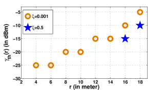
Figure 2: Relaying only via last placed relay: $\gamma_{th}(r)$ vs. $r$, for various relay costs, $\xi$, for the numerical example described in Section III-A6.

III-A7 Deployment Failure

Since, in practice, there is a maximum power at which a transmitter can transmit (e.g., 3 dBm), there is a possibility that a deployment can fail. It is interesting to compute the probability of such failure in the algorithms that we have derived. Here we provide a simulation estimate of the deployment failure probabilities for the sum power objective, under the threshold policies obtained numerically in Section III-A6. In our numerical example in Section III-A6, deployment failure can occur in the following two cases: (i) at $r=10$ steps the required power exceeds 3 dBm; the probability of this event is $2.65\%$ , and (ii) the source at the end of the line requires more than 3 dBm power. By simulating 200000 deployments, we observe that the deployment failure probability for $\xi=0.001,0.01,0.1$ and $1$ are $0.025\%,0.057\%,0.555\%$ and $3.8\%$ respectively.

Evidently, there is a trade-off between the target link performance and the probability of link failure. In addition, by placing relays more frequently, we reduce the chance of being caught in a situation where the deployment operative has walked too far without placing a relay and is unable to get a workable link to the previous node. In future work, we propose to include deployment failure probability as a constraint in the optimization formulation. Another way to reduce deployment failure is to permit back-tracking by the deployment operative, which, of course, will require the placement algorithm to keep more measurement history; we propose to permit this in our future work as well.

III-B Max-Power Objective

III-B1 Problem Formulation

We aim to address the following problem:

$$\min_{\pi\in\Pi}\mathbb{E}_{\pi}\bigg{(}\max_{i\in\{1,2,\cdots,N+1\}}\Gamma^{(i,i-1)}+\xi N\bigg{)}$$ (9)

We formulate (9) as an MDP. The state of the system is $(r,\gamma,\gamma_{\textit{max}})$ where $r$ and $\gamma$ are the same as before, and $\gamma_{\textit{max}}$ is the maximum power used in all the previously established links. The action space is $\{\textit{place},\,\textit{do not place}\}$ as before. The cost structure is such that the power cost is incurred only after the source node is placed.

III-B2 Bellman Equation

The problem is again an infinite horizon total cost problem with countable state space, finite action space and nonnegative single-stage cost. Hence, by the same arguments as used in problem (1), the optimal value function $J_{\xi}(\cdot)$ satisfies the Bellman equation (6). At state $\mathbf{0}$, it is not optimal to place a relay. Hence, $J_{\xi}(\mathbf{0})=\theta\mathbb{E}(\Gamma_{1})+(1-\theta)\mathbb{E}J_{\xi}(1,\Gamma_{1},0)$.

At state $(r,\gamma,\gamma_{\textit{max}})$, if we place a relay, we incur a cost $\xi$ and in the next step the line ends with probability $\theta$ in which case a power cost of $\mathbb{E}\max\{\gamma,\gamma_{\textit{max}},\Gamma_{1}\}$ is incurred. If the line does not end in the next step, the next state becomes $(1,\gamma^{\prime},\max\{\gamma,\gamma_{\textit{max}}\})$ where $\gamma^{\prime}\sim G_{1}$, and a cost of $\mathbb{E}J_{\xi}(1,\Gamma_{1},\max\{\gamma,\gamma_{\textit{max}}\})$ is incurred. On the other hand, if we do not place a relay at state $(r,\gamma,\gamma_{\textit{max}})$, the line ends in the next step with probability $\theta$ in which case a power cost of $\mathbb{E}\max\{\gamma_{\textit{max}},\Gamma_{r+1}\}$ is incurred. If the line does not end in the next step, the next state will be $(r+1,\gamma^{\prime},\gamma_{\textit{max}})$ where $\gamma^{\prime}\sim G_{r+1}$.

III-B3 Value Iteration

The value iteration for this MDP is given by (7) with $J_{\xi}^{(0)}(r,\gamma,\gamma_{\textit{max}})=0$ for all $r$, $\gamma$, $\gamma_{\textit{max}}$.

Lemma 3

The iterates of the value iteration (7) converge to the optimal value function, i.e., $J_{\xi}^{(k)}(r,\gamma,\gamma_{\textit{max}})\uparrow J_{\xi}(r,\gamma,\gamma_{\textit{max}})$ for all $(r,\gamma,\gamma_{\textit{max}})$, as $k\uparrow\infty$.

Proof:

See Appendix A. ∎

III-B4 Policy Structure

Lemma 4

$J_{\xi}(r,\gamma,\gamma_{\textit{max}})$ is concave, increasing in $\xi$ and increasing in $r$, $\gamma$, $\gamma_{\textit{max}}$.

Proof:

See Appendix A. ∎

Theorem 2

Policy Structure: The conditions for optimal relay placement are:

1. If $\gamma\leq\gamma_{\textit{max}}$, place the relay when $r\geq r_{\textit{th}}(\gamma_{\textit{max}})$ where $r_{\textit{th}}(\gamma_{\textit{max}})$ is a threshold value.

2. If $\gamma>\gamma_{\textit{max}}$, place the relay when $\gamma\leq\gamma_{\textit{th}}(r,\gamma_{\textit{max}})$ where $\gamma_{\textit{th}}(r,\gamma_{\textit{max}})$ is a threshold value increasing in $r$ and $\gamma_{\textit{max}}$.

Proof:

See Appendix A. ∎

Discussion of the policy structure: When $\gamma\leq\gamma_{\textit{max}}$, we can postpone placement until the point beyond which the chance of getting a worse value of power becomes significant. For $\gamma>\gamma_{\textit{max}}$, waiting to place the relay may result in a better channel; there is a threshold $\gamma_{\textit{th}}(r,\gamma_{\textit{max}})$ such that $\gamma_{\textit{th}}(r,\gamma_{\textit{max}})$ may cross $\gamma_{\textit{max}}$ for large enough $r$. If $\gamma$ is between these two values then we place.

III-B5 Computation of the Optimal Policy

Let us define $V_{\xi}(r,\gamma_{\textit{max}}):=\mathbb{E}J_{\xi}(r,\Gamma_{r},\gamma_{\textit{max}})$. We can again argue that the following function iteration (similar to that used in Section III-A)) will yield $V_{\xi}(r,\gamma_{\textit{max}})$ for all $r$, $\gamma_{\textit{max}}$, from which we can compute $r_{\textit{th}}(\gamma_{\textit{max}})$ and $\gamma_{\textit{th}}(r,\gamma_{\textit{max}})$:

$$V_{\xi}^{(k+1)}(r,\gamma_{\textit{max}}) = \sum_{\gamma}g(r,\gamma)\min\bigg{\{}\xi+\theta\mathbb{E}\max\{\gamma,\gamma_{\textit{max}},\Gamma_{1}\}$$ (10)

$$+ (1-\theta)V_{\xi}^{(k)}(1,\max\{\gamma,\gamma_{\textit{max}}\}),$$

$$\theta\mathbb{E}\max\{\gamma_{\textit{max}},\Gamma_{r+1}\}$$

$$+ (1-\theta)V_{\xi}^{(k)}(r+1,\gamma_{\textit{max}})\bigg{\}}$$

with $V_{\xi}^{(0)}(r,\gamma_{\textit{max}})=0$ for all $r$, $\gamma_{\textit{max}}$.

	$\xi=0.001$	$\xi=0.01$	$\xi=0.1$
$\mathbb{E}(N)$	18.1178	8.6875	4.6615
Relay Cost	0.01812	0.08688	0.46615
Power Cost	0.01524	0.04436	0.15079
$J_{\xi}(\mathbf{0})$	0.03336	0.13124	0.61693

TABLE II: Relaying via the last placed relay: break-up of the optimal cost for the example in Section III-B, for three values of the relay cost $\xi$.

III-B6 A Numerical Example

Figure 3 shows the variation of $r_{\textit{th}}(\gamma_{\textit{max}})$ with $\gamma_{\textit{max}}$ and $\xi$. Here we consider the same setting as Section III-A6. The plot shows that $r_{\textit{th}}(\gamma_{\textit{max}})$ increases with $\gamma_{\textit{max}}$. To get an insight into the reason, let us consider the situation $\gamma<\gamma_{\textit{max}}$. If $r$ is small, then it is more likely that in the next step also the power required to establish a link to the last node will be below $\gamma_{\textit{max}}$, and hence, we don’t need to place a relay. But if $r$ is large, then it is more likely that the required power will cross $\gamma_{\textit{max}}$ in the next step, and hence we will have a threshold $r_{\textit{th}}(\gamma_{\textit{max}})$ beyond which we have to place the relay. As $\gamma_{\textit{max}}$ increases, the probability that the power required to establish a link to the last node exceeding $\gamma_{\textit{max}}$ decreases for each $r$, thereby increasing $r_{\textit{th}}(\gamma_{\textit{max}})$. Also, $r_{\textit{th}}(\gamma_{\textit{max}})$ increases with $\xi$ because if the price of a relay increases, we will place relays less frequently.

Figure 4 shows the variation of $\gamma_{th}(r,\gamma_{max})$ with $r$ for $\gamma_{max}=-20$ dBm and two different values of $\xi$. For very small $\xi$ (e.g., $\xi=0.00001$), $\gamma_{th}(r,\gamma_{max})$ can be more than $\gamma_{max}$ for all $r$. For moderate values of $\xi$ (e.g., $\xi=0.01$ in Figure 3), $\gamma_{th}(r,\gamma_{max})$ vs. $r$ curve crosses $\gamma_{max}$ at $r=r_{th}(\gamma_{max})$. Also, we have seen numerically that for $\xi$ very large, $\gamma_{th}(r,\gamma_{max})$ is $0$ mW for $r\leq 9$ steps; for large $\xi$ we will place a relay only when $r=10$ steps ($20$ meters).

The variation of the mean number of relays $\mathbb{E}(N)$ and different cost components with $\xi$ is shown in Table II. It shows that as the cost of a relay $\xi$ increases, the mean number of relays decrease, and the power cost and $J_{\xi}(\mathbf{0})$ increase. Note that, for any given deployment and any given relay cost $\xi$, the sum power is always greater than the max power in the network. Hence, for a given $\xi$, the mean power cost and $J_{\xi}(\mathbf{0})$ for the sum power objective will be greater than the corresponding values for the max-power objective, as seen in Table I and Table II.

The estimated probability of deployment failure obtained from 200000 simulations of the deployment for $\xi=0.001,0.01,0.1$ and $1$ are $0.01\%,0.145\%,0.73\%$ and $5.39\%$ respectively.

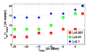
Figure 3: Relaying only via last placed relay: $r_{\textit{th}}(\gamma_{\textit{max}})$ vs. $\gamma_{\textit{max}}$, for various relay costs, $\xi$, for the numerical example described in Section III-B6.

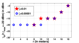
Figure 4: Relaying only via last placed relay: $\gamma_{th}(r,\gamma_{max})$ vs. $r$, for $\gamma_{max}=-20$ dBm and various relay costs, $\xi$, for the numerical example described in Section III-B6.

IV Relaying via Any Previous Node

In Section III, we considered the case where, after the deployment is over, only the links between adjacent nodes are permitted, i.e., only the links represented by the solid lines in Figure 1 can be used. However, as discussed in Section II, while formulating the problem we need to take into account the fact that some relays might be skipped after deployment, i.e., some of the links represented by the dotted lines in Figure 1 can be used. This section is dedicated to such formulation and exploration of the structural properties of the relay placement policies for different objectives.

IV-A Sum-Power Objective

IV-A1 Problem Definition

$$J_{\xi}\bigg{(}\{y_{k}\}_{k=1}^{n};\{P^{(k)}\}_{k=1}^{n};\{\gamma^{(k)}\}_{k=1}^{n}\bigg{)}=\min\bigg{\{}\xi+\theta\mathbb{E}\min\bigg{\{}\min_{k\in\{1,2,\cdots,n-1\}}(\Gamma_{y_{k}+1}+P^{(k)}),\Gamma_{1}+\min_{k\in\{1,2,\cdots,n\}}(\gamma^{(k)}+P^{(k)})\bigg{\}}$$ (11)

$$+ (1-\theta)\mathbb{E}J_{\xi}\bigg{(}1,y_{1}+1,\cdots,y_{n-1}+1;\min_{k\in\{1,\cdots,n\}}(\gamma^{(k)}+P^{(k)}),P^{(1)},\cdots,P^{(n-1)};\Gamma_{1},\Gamma_{y_{1}+1},\cdots,\Gamma_{y_{n-1}+1}\bigg{)},$$

$$\theta\mathbb{E}\min_{k\in\{1,\cdots,n\}}\bigg{(}\Gamma_{y_{k}+1}+P^{(k)}\bigg{)}+(1-\theta)\mathbb{E}J_{\xi}\bigg{(}\{y_{k}+1\}_{k=1}^{n};\{P^{(k)}\}_{k=1}^{n};\{\Gamma_{y_{k}+1}\}_{k=1}^{n}\bigg{)}\bigg{\}}$$

$$J_{\xi}\bigg{(}\{y_{k}\}_{k=1}^{m};\{P^{(k)}\}_{k=1}^{m};\{\gamma^{(k)}\}_{k=1}^{m}\bigg{)}=\min\bigg{\{}\xi+\theta\mathbb{E}\min\bigg{\{}\min_{k\in\{1,2,\cdots,m\}}(\Gamma_{y_{k}+1}+P^{(k)}),\Gamma_{1}+\min_{k\in\{1,2,\cdots,m\}}(\gamma^{(k)}+P^{(k)})\bigg{\}}$$ (12)

$$+ (1-\theta)\mathbb{E}J_{\xi}\bigg{(}1,y_{1}+1,\cdots,y_{m}+1;\min_{k\in\{1,\cdots,m\}}(\gamma^{(k)}+P^{(k)}),P^{(1)},\cdots,P^{(m)};\Gamma_{1},\Gamma_{y_{1}+1},\cdots,\Gamma_{y_{m}+1}\bigg{)},$$

$$\theta\mathbb{E}\min_{k\in\{1,\cdots,m\}}\bigg{(}\Gamma_{y_{k}+1}+P^{(k)}\bigg{)}+(1-\theta)\mathbb{E}J_{\xi}\bigg{(}\{y_{k}+1\}_{k=1}^{m};\{P^{(k)}\}_{k=1}^{m};\{\Gamma_{y_{k}+1}\}_{k=1}^{m}\bigg{)}\bigg{\}}$$

 

Given a deployment of $N$ relays, indexed $1,2,\cdots,N,$ consider the directed acyclic graph on these relays along with the sink (Node $0$) and the source (Node $N+1$), whose links are all directed edges from each node to every node with smaller index. Hence, if $i$ and $j$ are two nodes with $i>j$, there is only one link $(i,j)$ between them. Consider all directed acyclic paths from the source to sink, on this graph. Let us denote by $\mathbf{p}$ any arbitrary directed acyclic path from the source to the sink, and by $\mathbf{E}(\mathbf{p})$ the set of (directed) links of the path $\mathbf{p}$. We also define $\mathcal{P}_{n}:=\{\mathbf{p}:(i,j)\in\mathbf{E}(\mathbf{p})\implies i>j,|i-j|\leq n\}$ a subcollection of paths between the source and the sink on the directed acyclic graph, such that no path in $\mathcal{P}_{n}$ contains a link between two nodes whose indices differ by a number larger that $n$. We call $n$ the “memory” of the class of policies we are considering.

Here we consider the following problem:

$$\min_{\pi\in\Pi}\mathbb{E}_{\pi}\bigg{(}\min_{\mathbf{p}\in\mathcal{P}_{n}}\sum_{e\in\mathbf{E}(\mathbf{p})}\Gamma^{(e)}+\xi N\bigg{)}$$ (13)

where $\Gamma^{(e)}$ is the power used on the link $e$. We call $\sum_{e\in\mathbf{E}(\mathbf{p})}\Gamma^{(e)}$ the “length” of the path $\mathbf{p}$, and $\min_{\mathbf{p}\in\mathcal{P}_{n}}\sum_{e\in\mathbf{E}(\mathbf{p})}\Gamma^{(e)}$ the length of the “shortest path” from the source to the sink (over the relays deployed by policy $\pi$ in a given realization of the decision process).

$$J_{\xi}\bigg{(}\{y_{k}\}_{k=1}^{n};\{P^{(k)}\}_{k=1}^{n};\{\gamma^{(k)}\}_{k=1}^{n}\bigg{)}=\min\bigg{\{}\xi+\theta\mathbb{E}\min\bigg{\{}\min_{k\in\{1,2,\cdots,n-1\}}\max\{\Gamma_{y_{k}+1},P^{(k)}\},\max\{\Gamma_{1},\min_{k\in\{1,2,\cdots,n\}}\max\{\gamma^{(k)},P^{(k)}\}\}\bigg{\}}$$ (14)

$$+ (1-\theta)\mathbb{E}J_{\xi}\bigg{(}1,y_{1}+1,\cdots,y_{n-1}+1;\min_{k\in\{1,\cdots,n\}}\max\{\gamma^{(k)},P^{(k)}\},P^{(1)},\cdots,P^{(n-1)};\Gamma_{1},\Gamma_{y_{1}+1},\cdots,\Gamma_{y_{n-1}+1}\bigg{)},$$

$$\theta\mathbb{E}\min_{k\in\{1,\cdots,n\}}\max\{\Gamma_{y_{k}+1},P^{(k)}\}+(1-\theta)\mathbb{E}J_{\xi}\bigg{(}\{y_{k}+1\}_{k=1}^{n};\{P^{(k)}\}_{k=1}^{n};\{\Gamma_{y_{k}+1}\}_{k=1}^{n}\bigg{)}\bigg{\}}$$

$$J_{\xi}\bigg{(}\{y_{k}\}_{k=1}^{m};\{P^{(k)}\}_{k=1}^{m};\{\gamma^{(k)}\}_{k=1}^{m}\bigg{)}=\min\bigg{\{}\xi+\theta\mathbb{E}\min\bigg{\{}\min_{k\in\{1,2,\cdots,m\}}\max\{\Gamma_{y_{k}+1},P^{(k)}\},\max\{\Gamma_{1},\min_{k\in\{1,2,\cdots,m\}}\max\{\gamma^{(k)},P^{(k)}\}\}\bigg{\}}$$ (15)

$$+ (1-\theta)\mathbb{E}J_{\xi}\bigg{(}1,y_{1}+1,\cdots,y_{m}+1;\min_{k\in\{1,\cdots,m\}}\max\{\gamma^{(k)},P^{(k)}\},P^{(1)},\cdots,P^{(m)};\Gamma_{1},\Gamma_{y_{1}+1},\cdots,\Gamma_{y_{m}+1}\bigg{)},$$

$$\theta\mathbb{E}\min_{k\in\{1,\cdots,m\}}\max\{\Gamma_{y_{k}+1},P^{(k)}\}+(1-\theta)\mathbb{E}J_{\xi}\bigg{(}\{y_{k}+1\}_{k=1}^{m};\{P^{(k)}\}_{k=1}^{m};\{\Gamma_{y_{k}+1}\}_{k=1}^{m}\bigg{)}\bigg{\}}$$

 

IV-A2 MDP Formulation

Consider the evolution of the network as the relays are deployed. Suppose that at some point in the deployment process there are $m$ preceding nodes, including the sink; see Figure 5 where $m=4$. The transmit power required to establish a link from the current location to the $k$-th previous node is denoted by $\gamma^{(k)}$, and the distance of the current location from the $k$-th previous node is denoted by $y_{k}$. Let $P^{(k)}_{n}$ denote the length of the “shortest path” from the $k$-th previous node to the sink. We define $P^{(m)}_{n}:=0$ if $m\leq n$, i.e., the length of the shortest path from the sink to itself is $0$ (when $m\leq n$, the $m$-th previous node is the sink). For notational simplicity, we drop the subscript and denote $P^{(k)}_{n}$ by $P^{(k)}$. The deployment operative decides whether to place a node at his current position based on (i) the powers $\gamma^{(1)},\gamma^{(2)},\cdots,\gamma^{(n)}$, (ii) the distances $y_{1},y_{2},\cdots,y_{n}$, and (iii) the length of the shortest paths $P^{(1)},P^{(2)},\cdots,P^{(n)}$. If $n=2$, at the “current location” shown in Figure 6, the decision will be based on the powers $\gamma^{(1)}$, $\gamma^{(2)}$, the distances $y_{1}$, $y_{2}$, and the shortest paths $P^{(1)}$ and $P^{(2)}$ at nodes $3$ and $2$ respectively. However, in case $m<n$, we do not have measurements for $n$ previous nodes. Hence, let us define $l_{m}:=\min\{m,n\}$. At each step, the deployment operative knows the distance $\{y_{k}\}_{k=1}^{l_{m}}$, the power $\{\gamma^{(k)}\}_{k=1}^{l_{m}}$ and the lengths of the shortest paths $\{P^{(k)}\}_{k=1}^{l_{m}}$. He decides based on this information whether to place a relay at the current position or not. We formulate this problem as an MDP with state $(\{y_{k}\}_{k=1}^{l_{m}};\{P^{(k)}\}_{k=1}^{l_{m}};\{\gamma^{(k)}\}_{k=1}^{l_{m}})$, and the action space $\{\textit{place},\,\textit{do not place}\}$. The state at the sink is denoted by $\mathbf{0}$. Since the set $\mathcal{S}$ of transmit power levels is countable, $\{P^{(k)}\}_{k=1}^{l_{m}}$ also take values from a countable set. Hence, the state space is countable in our problem.

Figure 5: Measurement-based sequential relay placement. When standing at the “current location,” the deployment operative, having already deployed Relays $1$, $2$, and $3$, makes the power measurements $\gamma^{(k)}$, and knows the distances $y_{k}$.

Figure 6: Sequential deployment of relay nodes with $n=2$. When standing at the “current location,” the deployment operative, having already deployed Relays $1$, $2$, and $3$, makes the power measurements $\gamma^{(1)}$, $\gamma^{(2)}$, and knows the distances $y_{1}$, $y_{2}$ and the lengths $P^{(1)}$, $P^{(2)}$ of the shortest paths from relay $3$ and relay $2$ to the sink node.

If the state is $(\{y_{k}\}_{k=1}^{l_{m}};\{P^{(k)}\}_{k=1}^{l_{m}};\{\gamma^{(k)}\}_{k=1}^{l_{m}})$ and a relay is placed, the relay cost $\xi$ is incurred. The power cost is incurred only after the source is placed, and that cost will be the length of the shortest path in $\mathcal{P}_{n}$ from the source to the sink. Let us define $J_{\xi}(\{y_{k}\}_{k=1}^{l_{m}};\{P^{(k)}\}_{k=1}^{l_{m}};\{\gamma^{(k)}\}_{k=1}^{l_{m}})$ and $J_{\xi}(\mathbf{0})$ to be the optimal expected cost-to-go starting from state $(\{y_{k}\}_{k=1}^{l_{m}};\{P^{(k)}\}_{k=1}^{l_{m}};\{\gamma^{(k)}\}_{k=1}^{l_{m}})$ and state $\mathbf{0}$ respectively.

IV-A3 Bellman Equation

Note that here again we have an infinite horizon total cost MDP with a countable state space, finite action space and nonnegative single-stage cost. Hence, the optimal value function $J_{\xi}(\cdot)$ satisfies the Bellman equations (11) for $m\geq n$ and (12) for $m<n$, for the optimal cost function. The first term in the $\min\{\cdot,\cdot\}$ is the cost if we place a relay at the state $(\{y_{k}\}_{k=1}^{l_{m}};\{P^{(k)}\}_{k=1}^{l_{m}};\{\gamma^{(k)}\}_{k=1}^{l_{m}})$, and the second term is the cost if we do not place a relay.

Observe that it is never optimal to place a relay at state $\mathbf{0}$ because, in doing so, a cost $\xi$ will unnecessarily be incurred. Hence, $J_{\xi}(\mathbf{0})=\theta\mathbb{E}(\Gamma_{1})+(1-\theta)\mathbb{E}J_{\xi}(1;0;\Gamma_{1})$.

When $m\geq n$, if we place a relay at the current location and if the line ends in the next step, the length of the shortest path from the source to the sink will be seen as a terminal cost, and is equal to $\mathbb{E}\min\{\min_{k\in\{1,\cdots,n-1\}}(\Gamma_{y_{k}+1}+P^{(k)}),\Gamma_{1}+\min_{k\in\{1,\cdots,n\}}(\gamma^{(k)}+P^{(k)})\}$. Note that in this case the shortest path from the source to the sink can pass via the relay placed at the “current location”, or via one of the $(n-1)$ previous relays. For example, in the scenario shown in Figure 6 (with $n=2$), if we place a relay at the “current location” and the line ends at the next step, then the neighbouring node of the source along the shortest path can be the relay placed at the “current location” or relay $3$ (source is not allowed to transmit directly to relay $2$ because $n=2$). Keeping this in mind, $\Gamma_{y_{k}+1}+P^{(k)}$ is the sum of two costs: the (random) power $\Gamma_{y_{k}+1}$ from the source to the $(k+1)$-st previous node w.r.t the source (after placing the relay at the current location, the current $k$-th previous node will become the $(k+1)$-st previous node in the next step, where the source will be placed) and the length of the shortest path $P^{(k)}$ from that node to the sink. $\Gamma_{1}+\min_{k\in\{1,\cdots,n\}}(\gamma^{(k)}+P^{(k)})$ is the sum of the random power $\Gamma_{1}$ required to establish a link from the source to the relay deployed at the current location, and the length of the shortest path from this relay to the sink.

When $m\geq n$, if we place a relay at the current location and the line does not end in the next step, the terms $y_{n}$, $P^{(n)}$ and $\gamma^{(n)}$ disappear from the state (because a new relay has been placed, which must be taken into account in the state) and the distance $1$ of the next location from the newly placed relay at the current location is absorbed into the state. Other distances in the state increase by $1$ each. The length of the shortest path from the newly placed relay to the sink, i.e., $\min_{k\in\{1,\cdots,n\}}(\gamma^{(k)}+P^{(k)})$ enters the state, and the power required at the next location to connect to the $n$ previous relays (w.r.t the next location) are independently sampled again. Hence, keeping in mind that $\Gamma_{r}$ is the random power required to establish a link between two nodes at a distance $r$, the new state becomes:

$$(1,y_{1}+1,\cdots,y_{n-1}+1;\min_{k\in\{1,\cdots,n\}}(\gamma^{(k)}+P^{(k)}),$$

$$P^{(1)},\cdots,P^{(n-1)};\Gamma_{1},\Gamma_{y_{1}+1},\cdots,\Gamma_{y_{n-1}+1})$$

Similarly, if $m\geq n$ and we do not place a relay at the current location, in the next step the line may end with probability $\theta$ and may not end with probability $(1-\theta)$. If the line ends, a cost of the shortest path $\mathbb{E}\min_{k\in\{1,\cdots,n\}}(\Gamma_{y_{k}+1}+P^{(k)})$ will be incurred. If the line does not end, the next state will be the random tuple $(\{y_{k}+1\}_{k=1}^{n};\{P^{(k)}\}_{k=1}^{n};\{\gamma_{k}\}_{k=1}^{n})$, where for each $k\in\{1,\cdots,n\}$, $\gamma_{k}$ will be drawn independently from each other from the distribution $G_{y_{k}+1}(\cdot)$.

Similar arguments can be used to explain (12) in case $m<n$. The difference is that if we place a relay at the current location and the line does not end in the next step, the next state will have three more terms, since the information for the newly placed relay can be accomodated into the state. On the other hand, if the line ends in the next step, the source will be able to communicate to the sink via one of the $m$ relays (there will be $(m+1)$ preceding nodes, including the sink).

IV-A4 Results and Discussion

Theorem 3

Policy Structure: For the state $(\{y_{k}\}_{k=1}^{l_{m}};\{P^{(k)}\}_{k=1}^{l_{m}};\{\gamma^{(k)}\}_{k=1}^{l_{m}})$, the optimal relay placement policy is the following:

Place a relay if and only if $\min_{k\in\{1,\cdots,l_{m}\}}(\gamma^{(k)}+P^{(k)})\leq c(\{y_{k}\}_{k=1}^{l_{m}};\{P^{(k)}\}_{k=1}^{l_{m}})$ where $c(\{y_{k}\}_{k=1}^{l_{m}};\{P^{(k)}\}_{k=1}^{l_{m}})$ is a threshold value.

Proof:

See Appendix B. ∎

Discussion of the Policy Structure: The structure of the optimal policy as stated in Theorem 3 is intuitive because here we need to check whether the quantity $\min_{k\in\{1,\cdots,l_{m}\}}(\gamma^{(k)}+P^{(k)})$ which is the length of the shortest path from the current location of the deployment operative to the sink, is below a certain threshold.

Remarks:

• The optimal cost $J_{\xi}(\mathbf{0})$ of (13) is always less than or equal to that of (1), if the relay price $\xi$ is same in both cases. This is because each policy for $n=1$ will be a policy for $n=2$ as well.

• $n=\infty$ provides the best policy since there we consider information from all previous nodes.

Observation: With $n=1$, $r:=y_{1}$ and $\gamma:=\gamma^{(1)}$, the Bellman equation (11) reduces to:

$$J_{\xi}\bigg{(}r;P^{(1)};\gamma\bigg{)} = \min\bigg{\{}\xi+\theta\mathbb{E}(\Gamma_{1}+\gamma+P^{(1)})+$$ (16)

$$(1-\theta)\mathbb{E}J_{\xi}\bigg{(}1;(\gamma+P^{(1)});\Gamma_{1}\bigg{)},$$

$$\theta\mathbb{E}\bigg{(}\Gamma_{r+1}+P^{(1)}\bigg{)}$$

$$+ (1-\theta)\mathbb{E}J_{\xi}\bigg{(}r+1;P^{(1)};\Gamma_{r+1}\bigg{)}\bigg{\}}$$

Note that $J_{\xi}(r;P^{(1)};\gamma)=P^{(1)}+J_{\xi}(r;0;\gamma)$. Let us denote $J_{\xi}(r;0;\gamma):=J_{\xi}(r,\gamma)$. Now we can rewrite (16) as:

$$P^{(1)}+J_{\xi}\bigg{(}r,\gamma\bigg{)}=P^{(1)}+\min\bigg{\{}\xi+\gamma+\theta\mathbb{E}(\Gamma_{1})+\mathbb{E}J_{\xi}\bigg{(}1,\Gamma_{1}\bigg{)},$$

$$\theta\mathbb{E}\bigg{(}\Gamma_{r+1}\bigg{)}+(1-\theta)\mathbb{E}J_{\xi}\bigg{(}r+1,\Gamma_{r+1}\bigg{)}\bigg{\}}$$ (17)

Thus, we obtain the Bellman equation (3).

IV-B Max-Power Objective

Here we are going to address the following problem:

$$\min_{\pi\in\Pi}\mathbb{E}_{\pi}\bigg{(}\min_{\mathbf{p}\in\mathcal{P}_{n}}\max_{e\in\mathbf{E}(\mathbf{p})}\Gamma^{(e)}+\xi N\bigg{)}$$ (18)

We call $\max_{e\in\mathbf{E}(\mathbf{p})}\Gamma^{(e)}$ the “length” of the path $\mathbf{p}$, and $\min_{\mathbf{p}\in\mathcal{P}_{n}}\max_{e\in\mathbf{E}(\mathbf{p})}\Gamma^{(e)}$ the length of the “shortest path” from the source to the sink. Using notation and arguments similar to those used in problem (13), we can write the Bellman equations (14) and (15) and derive the structure of the optimal node placement policy:

Theorem 4

Policy Structure: For the state $(\{y_{k}\}_{k=1}^{l_{m}};\{P^{(k)}\}_{k=1}^{l_{m}};\{\gamma^{(k)}\}_{k=1}^{l_{m}})$, the optimal relay placement policy is the following:

Place a relay if and only if $\min_{k\in\{1,\cdots,l_{m}\}}\max\{\gamma^{(k)},P^{(k)}\}\leq c(\{y_{k}\}_{k=1}^{l_{m}};\{P^{(k)}\}_{k=1}^{l_{m}})$ where $c(\{y_{k}\}_{k=1}^{l_{m}};\{P^{(k)}\}_{k=1}^{l_{m}})$ is a threshold value.

Remark: Note that the Bellman equation (6) can be derived from (14), with $n=1$, $r:=y_{1}$, $\gamma:=\gamma^{(1)}$ and $P^{(1)}=\gamma_{max}$.

IV-C Performance comparison between $n=1$ and $n=2$

We have made a comparative study of the performance of the optimal policies with memory $1$ and the policies with memory $2$. The results are shown in Table III. Here we have used the same model as used in Section III in the max-power case, but we have considered $\mathcal{S}=\{0.1,0.2,\cdots,2\}$ mW in the sum-power case in order to avoid huge computational requirement. The study suggests that that, for small relay cost, $n=2$ can provide a significant percentage gain over the optimal cost for $n=1$. Since at small $\xi$ we tend to place more relays (but the relay cost is small compared to $J_{\xi}(\mathbf{0})$, see Table I and Table II), skipping relays could be useful. For large $\xi$, we place very few relays, but the relay cost will dominate. As $\xi$ becomes very high, we will always place the relays periodically at every $10$ steps, and nowhere else; hence the relay cost becomes independent of $n$. The little variation in power cost will be insignificant compared to large amount of relay cost.

	$\xi=0.001$	$\xi=0.01$	$\xi=0.1$	$\xi=1$
Sum-power	0.61946	0.65759	1.0414	4.49396
($n=1$)
Sum-power	0.50723	0.56834	1.0233	4.43836
($n=2$)
Max-power	0.03336	0.13124	0.61693	4.10798
($n=1$)
Max-power
($n=2$)	0.02119	0.10686	0.60548	4.09718

TABLE III: Comparison of $J_{\xi}(\mathbf{0})$ for $n=1$ and $n=2$ for different $\xi$: Sum-power objective and max-power objective. Two different transmit power sets are used for the two objectives.

IV-D Computational Issues

The dimension of the state space is $3n$ (increasing in $n$) in the value iteration, and hence the computational complexity and memory requirement increases with $n$. However, for any arbitrary $n$, we can reduce the value iteration to a function iteration in the same way as in (5) and (10), and reduce the dimension of the domain of the function to $2n$ (instead of $3n$ in the value iteration).

V Conclusion

In this paper, we explored several sequential relay placement problems for as-you-go deployment of wireless relay networks, assuming very light traffic. The problems were formulated as MDPs, optimal policies were derived, and the procedure illustrated via numerical examples. There are numerous issues to improve upon: (i) the light traffic (“lone packet model”) assumption, (ii) the assumption of independent shadow fading from link to link, and (iii) the deployment failure issue. Extension to positive traffic might require a different approach: perhaps one that requires a performance analysis model working in conjunction with an optimal sequential decision technique. We are addressing these issues in our ongoing work.

Appendix A Only Links between adjacent nodes permitted

Proof of Lemma 1: Here we have an infinite horizon total cost MDP with countable state space and finite action space. The assumption P of Chapter $3$ in [9] is satisfied since the single-stage cost is nonnegative. Hence, by combining Proposition $3.1.5$ and Proposition $3.1.6$ of [9], we obtain the result.

Proof of Lemma 2: In value iteration (4), $J_{\xi}^{(0)}(r,\gamma):=0$ is concave, increasing in $\gamma$, $\xi$ and increasing in $r$ and $J_{\xi}^{(0)}(\mathbf{0}):=0$ is concave, increasing in $\xi$. Suppose that $J_{\xi}^{(k)}(r,\gamma)$ is concave, increasing in $\gamma$, $\xi$ and increasing in $r$ and $J_{\xi}^{(k)}(\mathbf{0})$ is concave, increasing in $\xi$ for some $k\geq 0$. Note that $\mathbb{E}(\Gamma_{r+1})$ is increasing in $r$.

Let us consider $r_{1}>r_{2}$. We can write:

$$\mathbb{E}J_{\xi}^{(k)}(r_{1}+1,\Gamma_{r_{1}+1})$$

$$= \sum_{\gamma}g(r_{1}+1,\gamma)J_{\xi}^{(k)}(r_{1}+1,\gamma)$$

$$\geq \sum_{\gamma}g(r_{1}+1,\gamma)J_{\xi}^{(k)}(r_{2}+1,\gamma)$$

$$\geq \sum_{\gamma}g(r_{2}+1,\gamma)J_{\xi}^{(k)}(r_{2}+1,\gamma)$$

$$= \mathbb{E}J_{\xi}^{(k)}(r_{2}+1,\Gamma_{r_{2}+1})$$

where the first inequality follows from the fact that $J_{\xi}^{(k)}(r+1,\gamma)$ is increasing in $r$ for each $\gamma$, and the second inequality follows from the facts that $J_{\xi}^{(k)}(r+1,\gamma)$ is increasing in $\gamma$ and $G_{r}(\cdot)$ is stochastically increasing in $r$. Hence, $\mathbb{E}J_{\xi}^{(k)}(r+1,\Gamma_{r+1})$ is increasing in $r$. Hence, by (4), $J_{\xi}^{(k+1)}(r,\gamma)$ is increasing in $r$.

We know that the minimum of two concave, increasing functions is concave, increasing. Note that, each term in the $\min\{\cdot,\cdot\}$ of (4) is concave, increasing in $\gamma$, $\xi$. Hence, $J_{\xi}^{(k+1)}(r,\gamma)$ in concave, increasing in $\xi$, $\gamma$ and $J_{\xi}^{(k+1)}(\mathbf{0})$ is concave, increasing in $\xi$. Now, since $J_{\xi}^{(k)}(r,\gamma)\uparrow J_{\xi}(r,\gamma)$ for each $r$, $\gamma$ and $J_{\xi}^{(k)}(\mathbf{0})\uparrow J_{\xi}(\mathbf{0})$ (by Lemma 1), the results follow.

Proof of Theorem 1: By Proposition $3.1.3$ of [9], if there exists a stationary policy $\{\mu,\mu,\cdots\}$ such that for each state $(r,\gamma)$, the action chosen by the policy is the action that achieves the minimum in the Bellman equation (3), then that stationary policy will be an optimal policy. Hence, it is clear that when the state is $(r,\gamma)$, it is optimal to place the relay if $c_{p}\leq c_{np}$, i.e.,

$$\xi+\gamma+J_{\xi}(\mathbf{0})\leq\theta\mathbb{E}(\Gamma_{r+1})+(1-\theta)\mathbb{E}J_{\xi}\left(r+1,\Gamma_{r+1}\right)$$

or,

$$\gamma\leq\theta\mathbb{E}(\Gamma_{r+1})+(1-\theta)\mathbb{E}J_{\xi}\left(r+1,\Gamma_{r+1}\right)-(\xi+J_{\xi}(\mathbf{0}))$$

Thus, the condition for placing a relay when the state in $(r,\gamma)$ becomes $\gamma\leq\gamma_{\textit{th}}(r)$, where $\gamma_{\textit{th}}(r)$ is a threshold value. Now, by stochastic monotonicity of $\Gamma_{r}$ in $r$, $\mathbb{E}(\Gamma_{r+1})$ is increasing in $r$. Also, since $J_{\xi}(r,\gamma)$ is increasing in $r$, $\gamma$ and $\Gamma_{r}$ is stochastically increasing in $r$, $\mathbb{E}J_{\xi}\left(r+1,\Gamma_{r+1}\right)$ also is increasing in $r$. Hence, $\gamma_{\textit{th}}(r)$ is increasing in $r$.

Proof of Lemma 3: Here we have an infinite horizon total cost MDP with countable state space and finite action space. The assumption P of Chapter $3$ in [9] is satisfied since the single-stage cost is nonnegative. Hence, by combining Proposition $3.1.5$ and Proposition $3.1.6$ of [9], we obtain the result.

Proof of Lemma 4: Note that, in the value iteration (7), $J_{\xi}^{(0)}(r,\gamma,\gamma_{max}):=0$ is increasing in $r$, $\gamma$ and $\gamma_{max}$ and concave, increasing in $\xi$. Suppose that for some $k\geq 0$, $J_{\xi}^{(k)}(r,\gamma,\gamma_{max})$ is increasing in $r$, $\gamma$, $\gamma_{max}$ and concave, increasing in $\xi$. Since $J_{\xi}^{(k)}(r,\gamma,\gamma_{max})$ is increasing in $r$, $\gamma$ and $G_{r}(\cdot)$ is stochastically increasing in $r$, $\mathbb{E}J_{\xi}^{(k)}(r+1,\Gamma_{r+1},\gamma_{max})$ is increasing in $r$. $\mathbb{E}J_{\xi}^{(k)}(r+1,\Gamma_{r+1},\gamma_{max})$ is also increasing in $\gamma_{max}$, since $J_{\xi}^{(k)}(r,\gamma,\gamma_{max})$ is increasing in $\gamma_{max}$. $\mathbb{E}(\gamma_{max},\Gamma_{r+1})$ is increasing in $\gamma_{max}$ and also increasing in $r$ since $G_{r}$ is stochastically increasing in $r$. On the other hand, the first term in the $\min\{\cdot,\cdot\}$ of (7) is independent of $r$, but increasing in $\gamma$, $\gamma_{max}$ and linearly increasing in $\xi$. Now, minimum of two increasing functions is increasing and the minimum of a linear function and a constant is concave. Hence, $J_{\xi}^{(k+1)}(r,\gamma,\gamma_{max})$ is increasing in $r$, $\gamma$, $\gamma_{max}$ and concave, increasing in $\xi$. Since $J_{\xi}^{(k)}(r,\gamma,\gamma_{max})\uparrow J_{\xi}(r,\gamma,\gamma_{max})$, the results follow.

Proof of Theorem 2: By similar arguments as used in the proof of Theorem 1, the condition for placing a relay at a state $(r,\gamma,\gamma_{\textit{max}})$ is:

$$\xi+\theta\mathbb{E}\max\{\gamma,\gamma_{\textit{max}},\Gamma_{1}\}+(1-\theta)\mathbb{E}J_{\xi}(1,\Gamma_{1},\max\{\gamma,\gamma_{\textit{max}}\})$$

$$\leq\theta\mathbb{E}\max\{\gamma_{\textit{max}},\Gamma_{r+1}\}+(1-\theta)\mathbb{E}J_{\xi}(r+1,\Gamma_{r+1},\gamma_{\textit{max}})$$ (19)

Note that $\mathbb{E}\max\{\gamma_{\textit{max}},\Gamma_{r+1}\}$ increases in $r$. Also, $J_{\xi}(r+1,\gamma,\gamma_{\textit{max}})$ is increasing in $r$ and $\gamma$ for all $\gamma_{\textit{max}}$. Hence, $\mathbb{E}J_{\xi}(r+1,\Gamma_{r+1},\gamma_{\textit{max}})$ is increasing in $r$, since $G_{r}$ is stochastically increasing in $r$. Hence, the R.H.S of (19) is increasing in $r$ and $\gamma_{\textit{max}}$. Now, if $\gamma\leq\gamma_{\textit{max}}$, the L.H.S of (19) is independent of $\gamma$. Hence, the condition for placing the relay is $r\geq r_{\textit{th}}(\gamma_{\textit{max}})$ where $r_{\textit{th}}(\gamma_{\textit{max}})$ is a threshold value. On the other hand, if $\gamma>\gamma_{\textit{max}}$, the L.H.S of (19) is independent of $\gamma_{\textit{max}}$ and increasing in $\gamma$. Hence, we will place the relay if and only if $\gamma\leq\gamma_{\textit{th}}(r,\gamma_{\textit{max}})$ where $\gamma_{\textit{th}}(r,\gamma_{\textit{max}})$ is a threshold value increasing in $r$ and $\gamma_{\textit{max}}$.

Appendix B Links between any pair of nodes permitted

Proof of Theorem 3: By similar arguments using convergence of the value iteration as in the proof of Lemma 2, we can claim that $J_{\xi}(\{y_{k}\}_{k=1}^{l_{m}};\{P^{(k)}\}_{k=1}^{l_{m}};\{\gamma^{(k)}\}_{k=1}^{l_{m}})$ is increasing in each of its arguments. Now, the condition for placing a relay is that the first term in the $\min\{\cdot,\cdot\}$ of the R.H.S of (11) or (12) is less than or equal to the second term. Since the first term is increasing in $\min_{k\in\{1,\cdots,l_{m}\}}(\gamma^{(k)}+P^{(k)})$, the threshold nature of the optimal relay placement policy is evident.

References

- [1] M. Howard, M.J. Matarić, and S. Sukhat Gaurav. An incremental self-deployment algorithm for mobile sensor networks. Kluwer Autonomous Robots, 13(2):113–126, 2002.
- [2] M.R. Souryal, J. Geissbuehler, L.E. Miller, and N. Moayeri. Real-time deployment of multihop relays for range extension. In Proc. of the ACM International Conference on Mobile Systems, Applications and Services (MobiSys), San Juan, Puerto Rico, June 2007, pages 85–98. ACM, 2007.
- [3] Thorsten Aurisch and Jens Tölle. Relay Placement for Ad-hoc Networks in Crisis and Emergency Scenarios. In Proc. of the Information Systems and Technology Panel (IST) Symposium. NATO Science and Technology Organization, 2009.
- [4] Hengchang Liu, Jingyuan Li, Zhiheng Xie, Shan Lin, Kamin Whitehouse, John A. Stankovic, and David Siu. Automatic and robust breadcrumb system deployment for indoor firefighter applications. In Proc. of the ACM International Conference on Mobile Systems, Applications and Services (MobiSys), 2010.
- [5] A. Sinha, A. Chattopadhyay, K.P. Naveen, M. Coupechoux, and A. Kumar. Optimal sequential wireless relay placement on a random lattice path. http://arxiv.org/abs/1207.6318.
- [6] A. Bhattacharya and A. Kumar. QoS aware and survivable network design for planned wireless sensor networks. http://arxiv.org/abs/1110.4746.
- [7] M. Shaked and J.G. Shanthikumar. Stochastic Orders. Springer, 2006.
- [8] P. Mondal, K.P. Naveen, and A. Kumar. Optimal Deployment of Impromptu Wireless Sensor Networks. In Proc. of the IEEE National Conference on Communications (NCC),2012. IEEE, 2012.
- [9] D.P. Bertsekas. Dynamic Programming and Optimal Control, Vol. II. Athena Scientific, 2007.
- [10] E. Altman. Constrained Markov Decision Processes. Chapman and Hall/CRC; First Edition, 1999.