Snake states in graphene quantum dots in the presence of a p-n junction

Abstract

We investigate the magnetic interface states of graphene quantum dots that contain p-n junctions. Within a tight-binding approach, we consider rectangular quantum dots in the presence of a perpendicular magnetic field containing p-n, as well as p-n-p and n-p-n junctions. The results show the interplay between the edge states associated with the zigzag terminations of the sample and the snake states that arise at the p-n junction, due to the overlap between electron and hole states at the potential interface. Remarkable localized states are found at the crossing of the p-n junction with the zigzag edge having a dumb-bell shaped electron distribution. The results are presented as function of the junction parameters and the applied magnetic flux.

I Introduction

The study of graphene, a single layer of hexagonal carbon, has led to the discovery of new phenomena that highlight the unusual electronic properties of this 2D system Review . In particular, the linear gapless electronic spectrum, together with the chirality of carriers in this system is predicted to allow perfect transmission through potential barriers (Klein paradox) Katsnelson . This transmission has a directional character and is caused by the overlap between electron and hole states across the potential barrier milton0 ; falko . The effect has been investigated experimentally in p-n junctions of gated graphene samples Huard ; Williams ; Ozyilmaz ; Stander .

In the presence of an external magnetic field, the electron-hole overlap at the potential barrier (or p-n junction) causes the appearance of states that propagate along the junction interface milton1 ; Marcus1 . These are known as snake states since, in a semiclassical view, they arise through the coupling between counter-circling cyclotron orbits on either side of the p-n junction. They may also arise due to the presence of inhomogeneous fieldsorozlany and in warped and folded grapheneprada ; rainis . The presence of snake states was found to influence the electronic properties of graphene-based samples in the quantum Hall regime Marcus1 . Moreover, the coupling of snake states have been predicted to modify electrical current transport near the interfaces of narrow p-n-p junctions Levitov . Recently, experimental evidence was provided of the chaotic coupling of snake states in quantum point contactsMarcus2 .

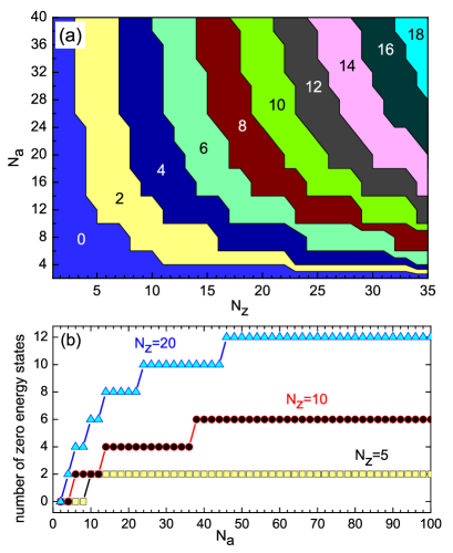
Figure 1: (Color online) (a) Number of nearly zero energy states within the interval $|E|<0.1$ meV as function of armchair ($N_{a}$) and zigzag ($N_{z}$) edge atoms. (b) Number of zero energies as function of $N_{a}$ for $N_{z}=5,10,20$.

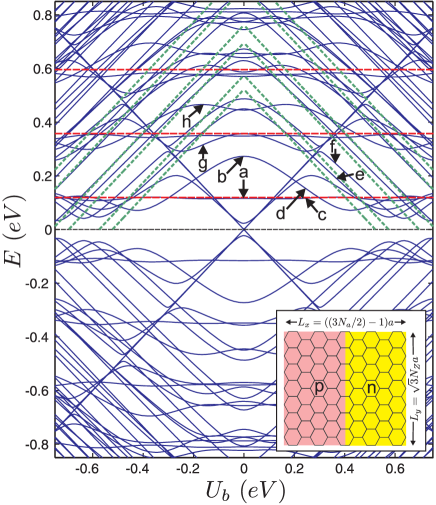
Figure 2: (Color online) Energy levels of a system with a p-n junction parallel to the zigzag edges in a rectangular GQD with $L_{x}=7.52$ nm, $L_{y}=8.6$ nm and $\Phi_{c}/\Phi_{0}=0$ as function of applied voltage $U_{b}$. The system is illustrated in the inset. The different colors represent the different gate voltages ($+U_{b}$ for p-type and $-U_{b}$ for n-type). The red dashed lines correspond to the energy states given by Eq. (3) and the green dashed lines represent the energy levels obtained from Eq. (4).

In this paper we investigate theoretically the interplay between edge and snake states of p-n, p-n-p, and n-p-n junctions imposed on graphene quantum dots (GQDs). We study the character of the different confined states by looking at the probability densities. The electron probability density can be linked to the local density of states (LDOS) which is a quantity that can be measured experimentally using scanning tunneling microscopy (STM). Measurement of the LDOS allows the probing of the spatial structure of the confined energy levels. Such measurements were recently reported for graphene quantum dotshmalainen . We consider GQDs created by cutting a larger graphene sample in order to obtain electronic confinement in a nanometer-scale structure with well-defined edges. The properties of the confined states of such GQDs in a magnetic field have been studied theoretically marko ; Ensslin0 as well as experimentally Ensslin2 . Note that such p-n junctions (but of irregular shape) are also naturally present in graphene samples when the Fermi energy is located around the Dirac point. They are generally known as puddles and have investigated with scanning tunneling microscopy (STM)martin ; deshpande ; zhangNa . In our calculations we neglect disorder which for the considered small sized dots will be of secondary importance.

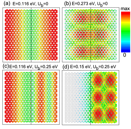
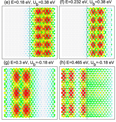
Figure 3: (Color online) Probability densities corresponding to the points indicated by (a-h) in Fig. 2. The black vertical line indicates the position of the p-n junction.

One important aspect of such graphene-based structures is the possible existence of edge states, for which the wavefunctions are localized at zigzag terminations of the sample Nakada ; Kohomoto ; Tang ; Zhang ; zarenia . These states have been recently observed by STMKobayashi ; Niimi . The presence of edge states can be especially relevant for nanometer-scale graphene structures. In particular, depending on the geometry of the GQDs, the edge states can correspond to the ground state of the system Zhang . For GQDs of general shape, Wimmer et al. have shown that the edge states tend to form a narrow band and are generally robust with regards to perturbations Guinea . In the present case we consider the effect of a position-dependent potential profile and an external perpendicular magnetic field on the energy spectrum of rectangular GQDs in the context of the nearest-neighbor tight-binding model. The presence of the potential interface thus introduces additional localized states, i.e. snake states, which can hybridize with the conventional zigzag edge states.

The paper is organized as follows: Section II gives a description of the model. In Sec. III we show and discuss the analytical and numerical results. Our summary and conclusions are presented in Sec. IV.

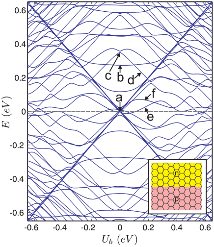
Figure 4: (Color online) Energy levels of a rectangular GQD with a p-n junction parallel to the armchair edges (see the inset of the figure) as function of applied electrostatic potential $U_{b}$ for the same parameters as Fig. 2.

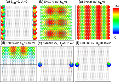
Figure 5: (Color online) Probability densities corresponding to the points indicated by (a-f) in Fig. 4. In panel (a) $E_{(8)}=0$ indicates the eighth degenerate zero energy. The black horizontal line indicates the position of the p-n junction.

II Model

The nearest-neighbor tight-binding Hamiltonian of the $\pi$ electrons in the honeycomb graphene lattice can be written as

$${\mathcal{H}}=\sum_{m}\epsilon_{m}c_{m}^{\dagger}c_{m}+\sum_{lm}(t_{lm}c_{l}^{\dagger}c_{m}+h.c.),$$ (1)

where $\epsilon_{m}$ is the on-site energy, $t_{lm}$ is the nearest-neighbor coupling parameter and $c_{j}$ ($c_{j}^{\dagger}$) is the annihilation (creation) operator of the electron at a site with label $j$. The external magnetic field introduces the Peierls phase in the coupling term $t_{lm}=t\exp\big{(}2\pi i\Phi_{l,m}\big{)}$, where $t$ is the zero-magnetic field coupling parameter, $\Phi_{l,m}=(1/\Phi_{0})\int_{r_{l}}^{r_{m}}{\mathbf{A}}\cdot{\mathbf{d}r}$, and $\Phi_{0}=h/e$ is the magnetic quantum flux and ${\mathbf{A}}$ is the vector potential. For graphene one has $t=2.7$ eV. The field is given by ${\mathbf{B}}=B$ẑ and we choose the Landau gauge as ${\mathbf{A}}=(0,Bx,0)$. Then, the Peierls phase for a transition between two sites $l$ and $m$ is $\Phi_{l,m}=0$ in the $x$ direction and $\Phi_{l,m}=\pm(x/3a)\Phi_{c}/\Phi_{0}$ along the $\pm y$ direction, where $\Phi_{c}=3\sqrt{3}a^{2}B/2$ is the magnetic flux threading one carbon hexagon with $a=0.142$ nm being the C-C distance. The p-n, p-n-p or n-p-n junctions are modeled by assuming a position-dependent on-site energy $\epsilon_{m}=\epsilon(m)$. Throughout this paper we assign the values $\epsilon=U_{b}$ ($\epsilon=-U_{b}$) for the p (n) regions, whereas at the interfaces between these regions the potential is assumed to vary abruptly. This assumption is expected not to influence the results qualitatively.

III p-n junction: zero magnetic field

We consider an almost square quantum dot because it allows us to investigate the effect of both armchair and zigzag edges in the same sample. We are interested to learn how the confined states are influenced by the relative orientation of the p-n interface with respect to the specific type of edges. Here, the length of the rectangular GQD which is terminated by armchair edges is defined as $L_{x}=[(3N_{a}/2)-1]a$ and the length terminated at the zigzag edges is $L_{y}=N_{z}\sqrt{3}a$ where $N_{a}$ and $N_{z}$ are the number of C-atoms, respectively at the armchair and zigzag edges. The total number of C-atoms in the rectangular GQD is $N=N_{a}(2N_{z}+1)$. We should notice that the energy spectrum of a rectangular GQD exhibits zero energy statesKim which are confined at the zigzag edges. The number of zero energy states in a rectangular dot depends to the number of both armchair and zigzag atomsKim . Figure 1(a) shows the number of states with nearly zero energies (we took the number of states within the energy interval $|E|<0.1$ meV) as function of $N_{z}$ and $N_{a}$. Our results show that for a fixed number of zigzag edge atoms the number of zero-energy states increases with increasing the armchair edge atoms (see Fig. 1(b)). Notice that the number of zero-energy states can not exceed $2N_{z}$.

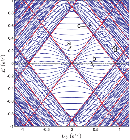
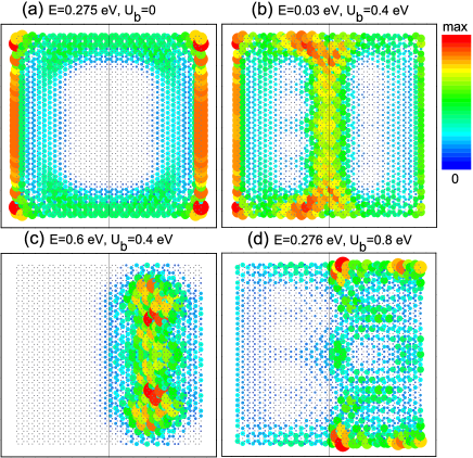
Figure 6: (Color online) Upper panel: The same as Fig. 2 but with non-zero magnetic flux $\Phi_{c}/\Phi_{0}=0.1$. The red dashed lines are the LLs of an infinite graphene sheet which are shifted up (down) by $U_{b}$($-U_{b}$). Lower panels: Probability densities corresponding to the points indicated by (a-d) in the upper panel. The black vertical line indicates the position of the p-n junction.

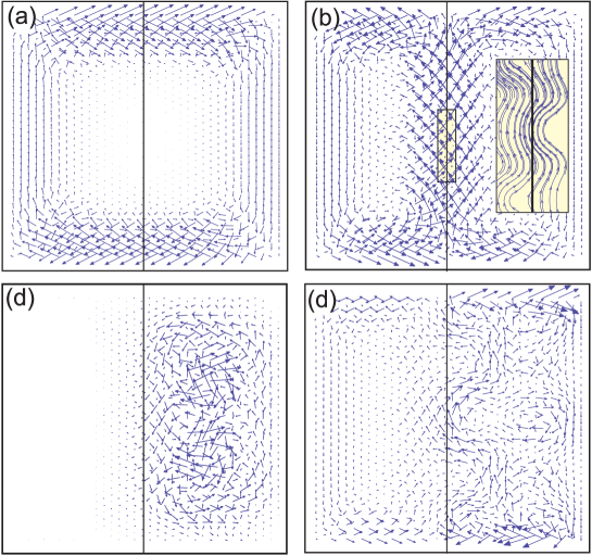
Figure 7: (Color online) Current density profile corresponding to the states indicated by (a-d) in Fig. 6. The black line indicates the position of the p-n junction. The inset in (b) shows a streamline plot of the enlargement region.

Now we solve the Hamiltonian (1) for a system in which a p-n junction is parallel to the zigzag edges of a rectangular GQD (see the inset of Fig. 2 where different colors represent the p-type and n-type regions which are respectively subjected to $+U_{b}$ and $-U_{b}$ gate voltages). For numerical purposes we take as an example $N_{a}=36$ ($L_{x}=7.52$ nm) and $N_{z}=35$ ($L_{y}=8.6$ nm) in all the results of this paper. The energy levels of this system are shown as function of the gate voltage $U_{b}$ in Fig. 2 for zero magnetic flux $\Phi_{c}/\Phi_{0}=0$. In the presence of a p-n junction parallel to the zigzag edges the zero energy-degenerate states split into two groups of degenerate states with energy: i) $E=+U_{b}$ and ii) $E=-U_{b}$ where the number of the states in each group is equal. Note that the energy spectrum in Fig. 2 exhibits a group of states which on average are almost independent of $U_{b}$. Figure 3 shows probability density plots for the states indicated by the letters (a-h) in Fig. 2. The probability densities in Fig. 3(a) and Fig. 3(c) exhibit a nodal character across the zigzag edges and consequently the $U_{b}$ energy shift from the p- and n-regions cancel out. These levels are similar to confined states in a zigzag nanoribbon. The energy levels of a zigzag nanoribbon are described, using the continuum model, by the transcendental equationbrey

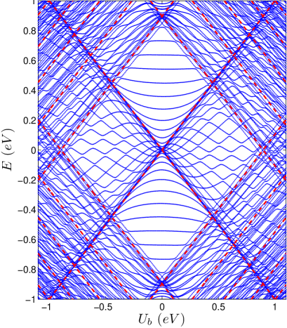
Figure 8: (Color online) The same as Fig. 4 but in the presence of magnetic flux $\Phi_{c}/\Phi_{0}=0.1$. The red dashed lines are the LLs of an infinite graphene sheet which are shifted up (down) by $U_{b}=0.25$ eV ($-U_{b}$).

$$\frac{k_{y}-\kappa}{k_{y}+\kappa}=e^{-2L_{x}\kappa}$$ (2)

where $\kappa=\sqrt{k_{y}^{2}-(\epsilon/\hbar v_{F})^{2}}$ with $v_{F}=10^{6}$ m/s being the Fermi velocity. In the low energy limit we take $k_{y}=0$ where Eq. (2) becomes $\displaystyle{\exp(\pm 2iL_{x}\epsilon/\hbar v_{F})}=-1$ and results in

$$\epsilon_{n}=\pm\frac{\pi\hbar v_{F}}{L_{x}}\big{(}n+\frac{1}{2}\big{)},~{}~{}~{}~{}n=0,1,2,...$$ (3)

The three first electronic levels of the above relation are shown in Fig. 2 by red dashed lines which coincide reasonable well with the position of the constant energy levels in the spectrum. Note that the agreement is better for low energy where the continuum model is more accurate. For the levels where the wavefunction is spread out inside the dot the energy levels are approximately linear with $U_{b}$. As seen in Figs. 3(b,d) the probability density corresponding to these levels shows an oscillatory behavior along the y-direction which is due to the confinement by the armchair edges. For armchair nanoribbons the wave vector $k_{y}$ satisfies the condition $k_{y}=(n_{y}\pi/L_{y})+(2\pi/3\sqrt{3}a)$ where $n_{y}$ being an integerbrey . Using Eq. (3) we take $k_{x}=\pi(n_{x}+1/2)/L_{x}$ along the x-direction. Thus the corresponding energies in the presence of $\pm U_{b}$ are proportional to $\pm(U_{b}\pm\hbar v_{F}\sqrt{k_{y}^{2}+k_{x}^{2}})$ which results in

$$\epsilon_{n}=\pm\left[U_{b}\pm\hbar v_{F}\sqrt{\big{(}\frac{n_{y}\pi}{L_{y}}+\frac{2\pi}{3\sqrt{3}a}\big{)}^{2}+\big{(}\frac{\pi(n_{x}+1/2)}{L_{x}}\big{)}^{2}}\right]$$ (4)

These electronic levels described by Eq. (4) which are shown by the green dashed lines in Fig. 2 for $-26\leq n_{y}\leq-20$ and $n_{x}=1$. The above arguments describe reasonably well qualitatively most of the energy levels that are found in the numerical spectrum depicted in Fig. 2. Because of the finite boundaries those levels may interact leading to anti-crossings. Aside from anti-crossings, the lines describe rather well the low energy levels in the spectrum that decrease linearly with $|U_{b}|$. Figs. 3(e,f) show the electronic density corresponding to the lowest paired levels for $U_{b}=0.38$ eV where the electrons are only confined in the $n$ region. Figures 3(g,h) show those states that are influenced by both zigzag and armchair edges.

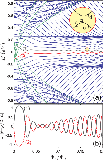
Figure 9: (Color online) (a) Energy levels of a rectangular GQD subjected to a p-n junction parallel to the zigzag edges (see the inset of Fig. 2) as function of magnetic flux threading one carbon hexagon $\Phi_{c}$ for $U_{b}=0.25$ eV. The green dashed curves are the Landau levels of an infinite graphene sheet which are shifted up (down) by $U_{b}$ ($-U_{b}$). (b) Persistent current corresponding to the first electron state (gray solid curve, labeled by (1)) and the first hole state (red dashed curve, labeled by (2)) as function of external magnetic flux $\Phi_{c}$.

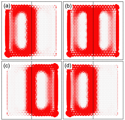
Figure 10: (Color online) Probability densities corresponding to the points indicated by (a-d) in the enlarged circle in Fig. 9(a). The black line indicates the position of the p-n junction.

The energy levels of a rectangular GQD subjected to a p-n junction parallel to the armchair edges is shown in Fig. 4. The system is depicted in the inset of Fig. 4. Since the p-n interface is now located perpendicular to the direction of the edge states (i.e. zigzag edges) the energy spectrum exhibits a complex behavior as function of $U_{b}$. In this case the spectrum is not symmetric under switching $U_{b}\rightarrow-U_{b}$ for $|E|<U_{b}$ which is due to the fact that the number of p-type and n-type atoms are unequal. The probability density corresponding to the points indicated by arrows are shown in Fig. 5. For $U_{b}=0$ and $E=0$ the carriers are confined at the zigzag edges (see Fig. 5(a) and the level is eighteen fold degenerate). Notice that the rectangular GQD with $N_{a}=36$ and $N_{z}=35$ has 16 zero energy states (see Fig. 1(a)). The probability density corresponding to the upper states are spread out over the dot in both x- and y-directions (see Fig. 5(b)) or along the zigzag edges (see Fig. 5(c)). In the presence of a p-n junction the electrons confine at the p(n)-region when $E>U_{b}$ and the energy state decrease(increase) with $U_{b}$ (Fig. 5(d)). In contrast with Fig. 2, for a p-n junction parallel to the armchair edge several states are found for $E<U_{b}$. These states, as seen in Figs. 5(e,f), present an interesting behavior: the probability densities show a significant localization at the intersection of the p-n interface and the zigzag edges. That can be explained as resulting from the hybridization of the zigzag edge states on each side of the p-n junction. This remarkable state appears only when the p-n junction crosses a zigzag edge. Note that the wavefunction of this state consists of both electron and hole components.

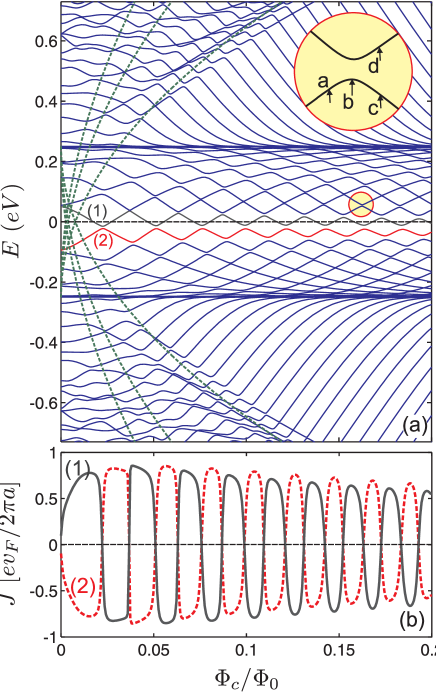
Figure 11: (Color online) The same as Fig. 9 but for a rectangular GQD subjected to a p-n junction parallel to the armchair edges (see the inset of Fig. 4)

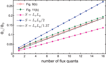
Figure 12: (Color online) The position of the oscillations in Figs. 9(b) and 11(b) and the number of flux quanta through the surface area $S=L_{x}L_{y},L_{x}L_{y}/2,S=L_{x}L_{y}/1.37$ as function of magnetic flux.

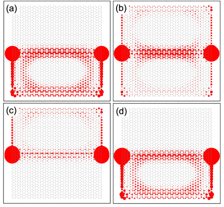
Figure 13: (Color online) Probability densities corresponding to the points indicated by (a-d) in the enlarged circle of Fig. 11(a). The black line indicates the position of the p-n junction.

IV snake states: influence of a perpendicular magnetic field

IV.1 p-n junction

In the presence of an external magnetic field (see upper panel in Fig. 6 for $\Phi_{c}/\Phi_{0}=0.1$) the energy spectrum shows anti-crossings for the energies below the gate voltage amplitude ($E<|U_{b}|$) which is due to the overlap between the quantum Hall (QH) edge states and the localized states at the p-n interface (i.e. snake states). Because of the smallness of the dot a large magnetic field (i.e. $B=800$ T for $\Phi_{C}/\Phi_{0}=0.1$) is required in order to have a significant influence on the energy levels. Nevertheless, as the influence of the magnetic field scales with the magnetic flux through the dot area, similar results will be obtained for lower magnetic fields if a larger graphene dot is considered. Notice that the number of degenerate levels with $E=\pm U_{b}$ ($E=0$) in the presence (absence) of a p-n junction does not change with magnetic field. The red dashed lines in Fig. 6 indicate the Landau levels (LLs) of an infinite graphene sheet that are shifted up(down) in the presence of an external potential $U_{b}$($-U_{b}$). The LLs are given by

$$E_{n}=sgn(n)\frac{3at}{2l_{B}}\sqrt{2|n|}\pm U_{b}$$ (5)

where $l_{B}=\sqrt{\hbar/eB}$ is the magnetic length and $n$ is an integerzarenia . Lower panels in Fig. 6 show the probability density corresponding to the states indicated by the arrows in the upper panel. Panel (a) shows the confinement due to the QH edge states and zigzag edge states for $U_{b}=0$. In the presence of a p-n junction and for $E<U_{b}$, states can arise due to the overlap of the QH edge states and the snake states (see panel (b)) or due to the overlap with confined states at the p (or n) regions (see panel (d)). For $E>U_{b}$ the carriers form LLs in the p (or n) potential regions (see panel (c)).

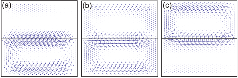
Figure 14: (Color online) Current density profile corresponding to the points indicated by (a-c) in the enlarged circle of Fig. 11(a). The black horizental line indicates the position of the p-n junction.

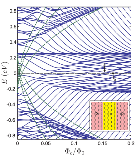
Figure 15: (Color online) Energy levels of a rectangular GQD with a p-n-p junction parallel to the zigzag edges as function of external magnetic flux for the same parameters as Fig. 9. The lower inset illustrates the system. The number of p-type atoms is twice larger than the number of n-type atoms. The green dashed curves are the LLs of an infinite graphene sheet which are shifted up (down) by $U_{b}$ ($-U_{b}$).

The different types of states become more apparent in Fig. 7 where we show the current density profile corresponding to the states shown in the lower panels of Fig. 6. The current density vectors are obtained using

$${\boldsymbol{j}_{l\rightarrow m}}=\frac{i}{\hbar}\big{[}\langle\psi_{l}|t_{lm}|\psi_{m}\rangle-\langle\psi_{m}|t_{lm}^{\ast}|\psi_{l}\rangle\big{]}$$ (6)

where ${\boldsymbol{j}_{l\rightarrow m}}$ is the current flowing out of site $l$ into site $m$. For clarity we show only the current corresponding to the A sublattice. Figures 7(b,d) clearly demonstrate the presence of snake states at the p-n junction where we have clockwise and counterclockwise circling currents, respectively, in the $n$ and $p$ regions. The current profile also reflects the direction of the bonds between the carbon atoms and therefore the arrows around the p-n junction sometimes point away from the interface. The streamline plot in the inset of Fig. 7(b) shows the current flow of the snake states more clearly. The vector plot in Fig. 7(a) indicates the cyclotron orbit of a quantum Hall edge state, while Fig. 7(c) shows the current profile of a LL state that is only very weakly influenced by the p-n junction and the edge of the quantum dot.

The energy levels as function of $U_{b}$ are shown in Fig. 8, in the presence of an external magnetic flux $\Phi_{c}/\Phi_{0}=0.1$ for the dot with p-n junction along the armchair edges (see the inset of Fig. 4). The red solid lines are the LLs of a graphene sheet (see Eq. (5)). As in Fig. 6(a) the energy spectrum exhibits different regimes of states; i) The regime of QH edge states where $U_{b}\leq|E|\leq E_{1}^{LL}$ and $E_{1}^{LL}$ is the first LL obtained from Eq. (5). ii) The $|E|\leq U_{b}$ and $|E|\leq E_{1}^{LL}$ regime where there exist snake states. iii) The regime of LLs form for $|E|\geq E_{i\geqslant 1}^{LL}$. Notice that for $U_{b}>0$ ($U_{b}<0$) the LLs form at p (n) region. iv) The last regime that can be seen in Fig. 8 (and Fig. 6(a)) is due to the overlap of the edge states and LLs that occurs when $E_{i\geqslant 1}^{LL}\leq|E|\leq U_{b}$.

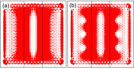
Figure 16: (Color online) (a) Electronic probability density and (b) the corresponding current profile for the points indicated by (a,b) in Fig. 15. The black vertical lines indicate the position of the p-n junctions.

Figure 9(a) displays the energy levels of the system illustrated in the inset of Fig. 2 as function of magnetic flux threading one carbon hexagon $\Phi_{c}$ for $U_{b}=0.25$ eV and the same size as Fig. 2. Notice that the zeroth Landau level in the absence of a gated voltage is now shifted up(down) by $+U_{b}$($-U_{b}$). The green dashed curves are LLs of an infinite graphene sheet (given by Eq. (5)). The magnetic levels in the GQD, i.e. the so called Fock Darwin levels, approach the LLsZhang ; Libisch which are shifted by $\pm U_{b}$. Some of the energy levels approach asymptotically the $E=\pm U_{b}$ levels. Due to the overlap between the QH edge states and the snake states at the p-n junction, anti-crossings appear in the energy spectrum. An anti-crossing point around $\Phi_{c}/\Phi_{0}=0.16$ is enlarged in Fig. 9(a). In Fig. 9(b) the persistent current corresponding to the first electron (solid curve) and the first hole (dashed curve) states is shown as function of magnetic flux. The persistent current $J$ is calculated by taking the derivative of the corresponding energy levels with respect to the flux as $J(\Phi_{c})=-\partial E/\partial\Phi_{c}$. Due to the anti-crossings in the energy spectrum, the persistent current exhibits an oscillatory behavior with respect to the magnetic flux. The current oscillation due to the snake states was recently investigated theoretically for a six-terminal graphene nano-ribbon with a p-n junctionChen . Notice that in the presence of the p-n junction the electron QH edge states that are shifted down with $-U_{b}$ overlap with the hole QH edge states that are shifted up with $U_{b}$ (they have an opposite circling orbit direction than the electronic QH edge states). This hybridize the states in the region $|E|\leq U_{b}$ and leads to the current oscillations. Thus, as the magnetic field is adiabatically increased, at each cycle of oscillation the electron becomes predominantly confined either on the p or the n sides of the quantum dot, with the current circulating either clockwise or counterclockwise.

Figure 10 shows the electron probability densities corresponding to the points indicated by (a-d) in the enlarged region of Fig. 9(a). Our results indicate that at the anti-crossing (panel (b)) the carriers are confined by the zigzag edge atoms and the p-n interface which characterizes the overlap between the edge and snake states. The points corresponding to the energy states that increase with respect to the magnetic flux around the anti-crossing (a,d) are due to states that are confined at the p-n junction and the zigzag edges in the n-type region (i.e. left side) while panel (c) displays an electron density that is confined at the right side of the p-n interface.

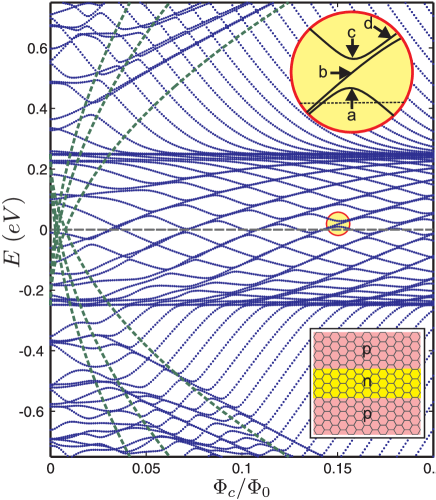
Figure 17: (Color online) The same as Fig. 15 but for a rectangular GQD with a p-n-p junction along the armchair edges. The system is illustrated in the lower inset.

The energy spectrum of the system depicted in the inset of Fig. 4 is shown in Fig. 11(a) as function of magnetic flux for $U_{b}=0.25$ eV. Since the number of p-type and n-type atoms are unequal here (where their minimum difference is $N_{a}$) the energy levels are not symmetric around $E=0$. Now the confinement due to the p-n junction is along the x-direction which is perpendicular to the edge states (caused by the zigzag edges). Therefore the energy spectrum exhibits a distinct behavior from that of the p-n junction along the zigzag edges. The persistent current $J$ corresponding to the energy levels indicated by (1) and (2) is shown in Fig. 11(b) as function of magnetic flux. Notice that the oscillatory behavior is different from the results in Fig. 9(b), now the current amplitude decreases smoothly with increasing magnetic flux. The position of the oscillations are plotted in Fig. 12 and compared with the flux through the quantum dot (magenta stars) and half of the quantum dot (blue triangles). Notice that the numerical results are between these two curves. It implies that the effective surface area encircled by the current is larger than the size of the $n$ or $p$ region. The best fit is obtained for flux through a surface area $S=L_{x}L_{y}/1.37$ (see gray squares).

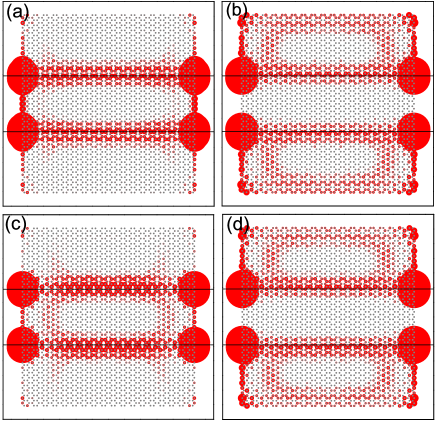
Figure 18: (Color online) Probability densities corresponding to the points indicated by (a-d) in the enlarged region of Fig. 17. The black horizontal line indicates the position of the p-n junctions.

Figure 13 shows the electron probability densities corresponding to the indicated points by (a,b,c,d) in the enlarged circle (an anti-crossing point around $\Phi_{c}/\Phi_{0}=0.16$) of Fig. 11(a). We have a superposition of three types of states: i) zigzag edge states (modified by the p-n junction), ii) QH edge states where we have skipping orbits, and iii) snake states. As seen in the figure the overlap of the confined electron in the snake state and the edge states leads to a large density at the intersection of the p-n junction and the zigzag edges. In contrast with the results in Fig. 10 only half of the zigzag edge atoms are contributing to the confinement due to the edge states. Therefore the carriers are weakly affected by the edge states in comparison with the confinement due to the snake states. At the anti-crossing (panel (b)) the electrons are mostly confined at the p-n interface and along both lengths of the zigzag edges. The corresponding current profiles of Figs. 13(a-c) are shown in Fig. 14. Figure 14(b) displays the snake states at the p-n interface and Figs. 14(a,c) show the cyclotron orbit of QH edge states respectively at the $p$ and $n$ regions.

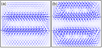
Figure 19: (Color online) Current density profile corresponding to the states shown in Fig. 18(a) and Fig. 18(b). The black horizontal lines indicate the position of the p-n junctions.

IV.2 p-n-p junction

Next we investigate the effect of multiple p-n junctions where we limit ourselves to the example of two junctions. We want to know if there can be any interplay between the two junctions, i.e. can states be confined over the two junctions? Will there be circling currents between the two junctions?

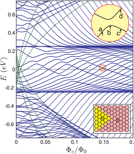
Figure 20: (Color online) Energy levels of a rectangular GQD with triangular shaped p-n junction as function of external magnetic flux for the same parameters as Fig. 9. The lower inset shows schematically the system. The green dashed curves are the LLs of an infinite graphene sheet which are shifted up (down) by $U_{b}$ ($-U_{b}$).

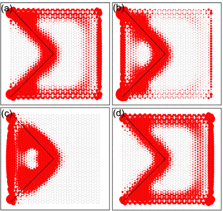
Figure 21: (Color online) Probability densities corresponding to the points indicated by (a-d) in the enlarged region of Fig. 20. The black line indicates the position of the p-n junction.

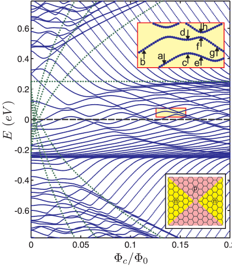
Figure 22: (Color online) Energy levels of a rectangular GQD with triangular shaped p-n-p junction as function of external magnetic flux for the same parameters as Fig. 9. The lower inset shows the system schematically where the yellow regions with zigzag edges indicate the n-type atoms. The green dashed curves are the LLs which are shifted up (down) by $U_{b}$ ($-U_{b}$).

A schematic illustration of a p-n-p junction in a rectangular GQD is depicted in the inset of Fig. 15 where the p-n-p junction is parallel to the zigzag edges (along y-direction). The corresponding spectrum in Fig. 15 exhibits quite distinct anti-crossings from the case of the p-n junction. On the other hand in low magnetic fields the hole edge states (i.e. those hole states that decrease with respect to the magnetic flux) do not approach the zeroth Landau Level ($E=-U_{b}$) which is a consequence of the fact that the n-type region does not have a boundary with the zigzag edges. Notice that the hole edge states approach $E=-U_{b}$ in high magnetic fields. The electron probability densities for the points indicated by (a) and (b) are shown in Figs. 16(a,b) where the densities are spread out mostly along the p-n and n-p interfaces. The corresponding current profiles are plotted in Figs. 16(c,d). Our results show opposite circling currents between the two junctions.

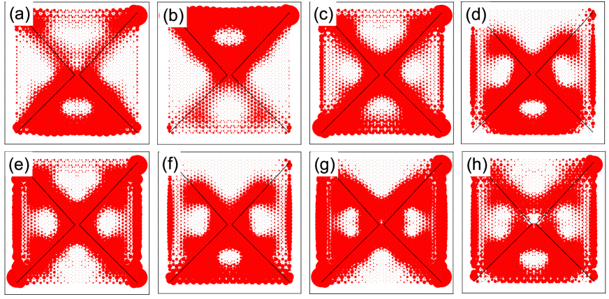
Figure 23: (Color online) Probability densities corresponding to the points indicated by (a-h) in the enlarged region of Fig. 22. The black lines indicate the position of p-n junctions.

Figure 17 displays the energy spectrum for the p-n-p junction parallel to the armchair edges in a rectangular GQD. The system is depicted in the lower inset. Here the n-type region is connected to the zigzag lengths which leads to the convergence of the hole edge states to $E=-U_{b}$ even in low magnetic fields. As in previous cases for the region $|E|<U_{b}$ anti-crossings appear in the spectrum. The electron probability densities corresponding to the points around the enlarged anti-crossing (yellow circle) are shown in Fig. 18. Note that the anti-crossing behaviour is qualitative distinct from the previous cases shown in Figs. 9(a) and 11(a). Our results indicate that at the anti-crossing (a,c) the electrons are confined due to the edge states corresponding to the zigzag atoms in the n-type region and the snake states. The points (b,d), correspond to states that ate confined at the zigzag edges in the p-type regions and near the p-n-p junction. In all points, the probability density shows strong peaks at the intersection of the p-n junction with the zigzag edges. The density profiles have a dumb-bell shape. As before, these localized states are associated with the hybridization of the zigzag edge states on each side of the junction. However, for non-zero magnetic field these states overlap with snake states that propagate along the potential interfaces. The current profile corresponding to Figs. 18(a,b) is shown in Fig. 19(a,b) where the counter-circling cyclotron orbits in the n and p regions demonstrate the existence of snake states at the p-n interfaces.

V Triangular shaped p-n junction

Next we consider the effect of the gate shape on the energy spectrum. Figure 20 displays the energy levels for the system illustrated in the lower inset where a triangle-shaped gate voltage is assumed for the n-type region. Notice that here we choose an arbitrary direction for the p-n junction and it not necessarily matched with the zigzag or armchair direction. Since the number of n-type and p-type atoms are unequal the electron and hole energy levels are not symmetric, i.e. $|E_{e}(\Phi_{c})|\neq|E_{h}(\Phi_{c})|$. Due to the confinement by both edge states (at zigzag edges) and snake states (at p-n interface) anti-crossings appear in the energy spectrum. An enlargement around one of the anti-crossings at $\Phi_{c}/\Phi_{0}=0.15$ is shown in the inset of Fig. 11(b). The electron probability densities for the points around this anti-crossing (a,b,c,d) are shown in Fig. 21. Panel (b) shows the electron density at the anti-crossing where the electrons confined along the zigzag edge and the p-n interface. For the points whose energy increases with flux (a,d) the electron is localized along the zigzag edge in the $p$ region and snake states are present along the p-n junction while the probability density for the point (c) is mostly along the zigzag edges in the n region and the p-n interface.

As a last example we investigate the energy spectrum of a system consisting of a point contact in a rectangular GQD (see the lower inset of Fig. 22). Recently, transport measurements of such a system were carried out, and it was found that, due to a chaotic mixing of edge channels an unexpected half-integer plateau was observed in the QH resistivityMarcus2 . The spectrum exhibits double anti-crossings between the energy levels in the region $|E|<U_{b}$. The enlarged rectangle in Fig. 22 shows one of these double-anticrossings around $\Phi_{c}/\Phi_{0}\approx 0.15$. Figure 23 shows the electron probability densities corresponding to the points indicated by a-h in Fig. 22. The energy levels between $-U_{b}$ and $U_{b}$ that increase with magnetic flux are due to the overlap of the QH edge states in the p region and the snake states at the p-n interface (Figs. 23(a,b)). Those energy levels that decrease with magnetic flux correspond to the zigzag edge states which hybridize with the QH edge states in the n-region and to snake states (Figs. 23(e,g)). Notice that at the anti-crossings, see Figs. 23(c,d,f,h), we have an overlap of three types of localized states (i.e. QH edge states, snake states and zigzag edge states).

VI Concluding remarks

We presented numerical results for the energy spectrum and magnetic field dependence of the eigenstates of graphene-based quantum dots, on which p-n junctions create electron and hole-doped regions. The presence of the magnetic field, together with the coupling between electron and hole states across the potential barrier due to Klein tunneling leads to the appearance of localized states at the potential interface, known as snake states. These states, which have previously been investigated for pn junctions on infinite graphene sheets, can influence the transport properties of graphene-based nanodevices. We have obtained results that show that for the case of quantum dots the low energy dynamics of the system is dominated by hybridized states that arise due to the overlap between quantum Hall edge states and the snake states at the p-n junction, with the snake states allowing the superposition of quantum Hall edge states at the p and n sides of the dot. These states are characterized by an energy spectrum that displays an oscillating behavior as function of the electrostatic potential and magnetic field at the vicinity of the Fermi energy. Furthermore, the energy spectrum was shown to depend on the specific alignment of the potential interfaces with regard to the graphene lattice, as well as on the geometry of the gates. The dots were assumed to be defect-free and to have perfect zigzag or armchair edges. Future work shall concentrate on the effect of edge disorder, impurities and defects on the electronic properties of these structures. Another aspect that shall be considered is the influence of the particular choice of the potential profile and shape of the graphene flake on the confined states.

VII Acknowledgment

This work was supported by the Flemish Science Foundation (FWO-Vl), the European Science Foundation (ESF) under the EUROCORES program EuroGRAPHENE (project CONGRAN), the Brazilian agency CNPq (Pronex), and the bilateral projects between Flanders and Brazil and the collaboration project FWO-CNPq.

References

- (1) A. H. Castro Neto, F. Guinea, N. M. R. Peres, K. S. Novoselov, and A. Geim, Rev. Mod. Phys. 81, 109 (2009).
- (2) M. I. Katsnelson, K. S. Novoselov, and A. K. Geim, Nature Physics 2, 9, 620 (2006).
- (3) V. V. Cheianov and V. I. Fal´ko, Phys. Rev. B 74, 041403(R) (2006).
- (4) J. M. Pereira Jr., V. Mlinar, F. M. Peeters, and P. Vasilopoulos, Phys. Rev. B 74, 045424 (2006).
- (5) B. Huard, J. A. Sulpizio, N. Stander, K. Todd, B. Yang, and D. Goldhaber-Gordon, Phys. Rev. Lett. 98, 236803 (2007).
- (6) J. R. Williams, L. DiCarlo, and C. M. Marcus, Science 317, 638 (2007).
- (7) B. Özyilmaz, P. Jarillo-Herrero1, D. Efetov, D. A. Abanin, L. S. Levitov, and Philip Kim, Phys. Rev. Lett. 99, 166804 (2007).
- (8) N. Stander, B. Huard, and D. Goldhaber-Gordon, Phys. Rev. Lett. 102, 026807 (2009).
- (9) J. M. Pereira Jr., F. M. Peeters, and P. Vasilopoulos, Phys. Rev. B 75, 125433 (2007).
- (10) J. R. Williams and C. M. Marcus, Phys. Rev. Lett. 107, 046602 (2011).
- (11) L. Oroszlány, P. Rakyta, A. Kormányos, C. J. Lambert, and J. Cserti, Phys. Rev. B 77, 081403 (2008); T. K. Ghosh, A. De Martino, W. Häusler, L. Dell’Anna, and R. Egger, Phys. Rev. B 77, 081404 (2008).
- (12) E. Prada, P. San-Jose, and L. Brey, Phys. Rev. Lett. 105, 106802 (2010).
- (13) D. Rainis, F. Taddei, M. Polini, G. León, F. Guinea, and V. I. Fal´ko, Phys. Rev. B 83, 165403 (2011).
- (14) D. A. Abanin and L. S. Levitov, Science 317, 641 (2007).
- (15) S. Nakaharai, J. R. Williams, and C. M. Marcus, Phys. Rev. Lett. 107, 036602 (2011).
- (16) S. K. Hmäläinen, Zh. Sun, Mark P. Boneschanscher, A. Uppstu, M. Ijäs, A. Harju, D. Vanmaekelbergh, and P. Liljeroth, Phys. Rev. Lett. 107, 236803 (2011).
- (17) M. Grujić, M. Zarenia, A. Chaves, M. Tadić, G. A. Farias, and F. M. Peeters, Phys. Rev. B 84, 205441 (2011).
- (18) S. Schnez, K. Ensslin, M. Sigrist, and T. Ihn, Phys. Rev. B 78, 195427 (2008).
- (19) J. Güttinger, C. Stampfer, F. Libisch, T. Frey, J. Burgd rfer, T. Ihn, and K. Ensslin, Phys. Rev. Lett. 103, 046810 (2009).
- (20) J. Martin, N. Akerman, G. Ulbricht, T. Lohmann, J. H. Smet, K. von Klitzing, and A. Yacoby, Nat. Phys. 4, 144 (2008).
- (21) A. Deshpande, W. Bao, F. Miao, C. N. Lau, and B. J. LeRoy, Phys. Rev. B 79, 205411 (2009).
- (22) Y. Zhang, V. W. Brar, C. Girit, A. Zettl, and M. F. Crommie, Nat. Phys. 5, 722 (2009).
- (23) K. Nakada, M. Fujita, G. Dresselhaus, and M. S. Dresselhaus, Phys. Rev. B 54, 17954 (1996).
- (24) M. Kohomoto and Y. Hasegawa, Phys. Rev. B 76, 205402 (2007).
- (25) C. Tang, W. Yan, Y. Zheng, G. Li, and L. Li, Nanotechnology 19, 435401 (2008).
- (26) M. Zarenia, A. Chaves, G. A. Farias, and F. M. Peeters, Phys. Rev. B 84, 245403 (2011).
- (27) Z. Z. Zhang, Kai Chang, and F. M. Peeters, Phys. Rev. B 77, 235411 (2008).
- (28) Y. Kobayashi, K. Fukui, T. Enoki, K. Kusakabe, and Y. Kaburagi, Phys. Rev. B 71, 193406 (2005).
- (29) Y. Niimi, T. Matsui, H. Kambara, K. Tagami, M. Tsukada, and Hiroshi Fukuyama, Phys. Rev. B 73, 085421 (2006).
- (30) M. Wimmer, A. R. Akhmerov, and F. Guinea, Phys. Rev. B 82 045409 (2010).
- (31) S. C. Kim, P. S. Park, and S. R. Eric Yang, Phys. Rev. B 81, 085432 (2010).
- (32) L. Brey and H. A. Fertig, Phys. Rev. B 73, 235411 (2006).
- (33) F. Libisch, S. Rotter, J. Güttinger, C. Stampfer, and J. Burgdörfer, Phys. Rev. B 81, 245411 (2010).
- (34) Jiang-chai Chen, X. C. Xie, and Qing-Feng Sun, Phys. Rev. B 86, 035429 (2012).