Time delays and advances in classical and quantum systems

Abstract

The paper reviews positive and negative time delays in various processes of classical and quantum physics. In the beginning, we demonstrate how a time-shifted response of a system to an external perturbation appears in classical mechanics and classical electrodynamics. Then we quantify durations of various quantum mechanical processes. The duration of the quantum tunneling is studied. An interpretation of the Hartman paradox is suggested. Time delays and advances appearing in the three-dimensional scattering problem on a central potential are considered. Then we discuss delays and advances appearing in quantum field theory and after that we focus on the issue of time delays and advancements in quantum kinetics. We discuss problems of the application of generalized kinetic equations in simulations of the system relaxation towards equilibrium and analyze the kinetic entropy flow. Possible measurements of time delays and advancements in experiments similar to the recent OPERA neutrino experiment are also discussed.

1 Introduction

Many definitions of time, as a measure of a duration of a process, are possible in classical mechanics because for the measuring of the time duration any process is suitable, which occurs at a constant pace. Naively thinking, a response of a system to an external perturbation should be delayed in accordance with the causality principle. However, it is not always the case. There may arise both delays and advancements (negative time delays) in system responses without contradiction with causality.

Time delays and possible time advancements in quantum mechanical phenomena have been extensively discussed in the literature, see Refs. [1, 2, 3, 4, 5, 6, 7, 8, 9, 10, 11, 12] and references therein. In spite of that many questions still remain not quite understood. Worth mentioning is the Hartman effect [13], that the transition time of a quantum particle through a one-dimensional barrier is seemingly independent of the barrier length for broad barriers. This causes apparent superluminal phenomena in the quantum mechanical tunneling. Many, at first glance, supporting experiments with single photons, classical light waves and microwaves have been performed, see Refs. [14, 15, 16, 17, 18] and references therein. Different definitions of time delays, such as the group transmission time delay $\delta t_{\rm T}$, the group reflection time delay $\delta t_{\rm R}$, the interference time delay $\delta t_{\rm i}$, the dwell time $t_{\rm d}$, the sojourn time $t_{\rm soj}$, and some other quantities have been introduced to treat the problem. All these time scales suffer from the Hartmann effect and are in odd with the natural expectation that the tunneling time should be proportional to the length of the barrier. A re-interpretation consistent with special relativity suggested in [8] is that these times should be treated as the live times of the corresponding wave packets rather than the traveling time. If so, the so far performed experiments measured an energy dissipation at the edges of the barrier rather than a particle traveling time.

Additionally to the mentioned time delays other relevant time quantities were introduced, and the differences between the averaged scattering time delay $\delta t_{\rm s}$ and the Wigner scattering time delay $\delta t_{\rm W}$ were discussed in Ref. [3, 19, 20], see also Refs. [4, 5, 6] and references therein. Based on these analyses authors of Ref. [20] argued that kinetic simulations describing relaxation of a system, first, towards the local equilibrium and, then, towards the global one must account for delays in scattering events consistently with mean fields acting on particles, in order to model consistently thermodynamic properties of the system. For practical simulations, as the relevant relaxation time they suggested to use the scattering time delay $\delta t_{\rm s}$, as it follows from the phase shift analysis, rather than the collision time $t_{\rm col}$, as it appears in the original Boltzmann equation. A number of BUU simulations of heavy ion collision reactions were performed using this argumentation, see Ref. [21] and references therein.

The appropriate frame for the description of non-equilibrium many-body processes is the real-time formalism of quantum filed theory developed by Schwinger, Kadanoff, Baym and Keldysh [22, 23, 24, 25]. A generalized kinetic description of off-mass-shell (virtual) particles has been developed based on the quasiclassical treatment of the Dyson equations for non-equilibrium systems, see Refs. [24, 26, 27, 28, 29, 30, 31]. This treatment assumes the validity of the first-order gradient approximation to the Wigner-transformed Dyson equations. As it is ordinary sought, the gradient approximation is valid, if the typical time-space scales are much larger than the microscopic scales, such as $1/E_{\rm F}$ and $1/p_{\rm F}$ for a slightly excited Fermi systems, where $E_{\rm F}$ is the Fermi energy and $p_{\rm F}$ is the Fermi momentum. As the result, a quantum kinetic equation is derived for off-mass shell particles, for which the energy and momentum are not connected by any dispersion relation. We call this generalized kinetic equation the Kaddanoff-Baym (KB) equation. Among other terms, this equation contains the Poisson-bracket term, which origin has not been quite understood during a long time. Botermans and Malfliet in Ref. [32] suggested to replace the production rate in that Poisson-bracket term by its approximate quasi-equilibrium value. This allowed to simplify the KB equation for near equilibrium configurations. The resulting form of the kinetic equation is called the Botermans-Malfliet (BM) form. It is argued that the BM replacement does not spoil the validity of the first order gradient approximation. The so-called $\Phi$-derivable self-consistent approximations in the quantum field theory were introduced by Baym in Ref. [33] for quasi-equilibrium systems. His derivation was then generalized to an arbitrary Schwinger-Keldysh contour in Ref. [34]. Reference [35] developed the self-consistent treatment of the quantum kinetics. References [36, 37] demonstrated that the KB kinetic equation is compatible with the exact conservation of the Noether 4-current and the Noether energy-momentum, whereas the Noether 4-current and the Noether energy-momentum related to the BM form of equation are conserved only approximately, up to zeroth gradients. Fulfillment of the conservation laws is important in practical simulations of dynamical processes. For example, in kinetic simulations of heavy ion collisions the gradient approximation may not work at least on an initial stage of the expansion of the fireball. In this case the KB form of the kinetic equation should be preferable compared to the BM one due to inherent exact conservation laws for the Noether quantities in the former case. However, up to now the simulation scheme, the so called test particle method, has been realized in applications to heavy-ion collisions only for the BM form of the kinetic equation, see Refs. [38, 39, 21]. The relaxation time arising in the kinetic equation presented in the BM form is the scattering time delay, $\delta t_{\rm s}$, rather than the average collision time $t_{\rm col}$, as it appears in the original KB equation. Since $\delta t_{\rm s}$ can be naturally interpreted in terms of the virial expansion [20], this was considered as an argument in favor of the BM form of the kinetic equation.

Recent work [40] suggested a non-local form of the quantum kinetic equation, which up to second gradients coincides with the KB equation and up to first gradients, with the BM equation. Thus, the non-local form keeps the Noether 4-current and Noether energy-momentum conserved at least up to first gradients. Second advantage of the non-local form is that it allows interpretation of mentioned difference in the Poisson-bracket terms in the KB and BM equations, as associated with space-time and energy-momentum delays and advancements. Also the non-local form of the kinetic equation permits, in principle, to develop a test particle method, similar to that is used for the BM form of the kinetic equation.

In this paper we study problems related to determination of time delays and advancements in various phenomena. In Sect. 2 we discuss how time delays and lesser time advancements arise in the description of oscillations in classical mechanics and in classical field theory of radiation. In Sect. 3 we consider time delays and advancements in one-dimensional quantum mechanical tunneling and in scattering of particles above the barrier. Problem of an apparent superluminality in the tunneling (the Hartman effect) is considered and a solution of the paradox is suggested. In Sect. 4 we consider time delays and advancements in the three-dimensional scattering problem. Then in Sect. 5 we introduce the non-equilibrium Green’s function formalism and show that not only space-time delays but also advancements appear in Feynmann diagrammatic description of quantum processes within the quantum field theory. In Sect. 6 we focus on the quasiclassical description of non-equilibrium many-body phenomena. We introduce gradient expansion scheme and arrive at a set of equations for the kinetic quantities, which should be solved simultaneously. The kinetic equation for the Wigner density is presented in three different forms, the KB, the BM and the non-local form. We discuss time delays and advancements, as they appear in the non-local form of the kinetic equation (and in the KB equation equivalent to it up to the second-order gradient terms) and consider their relation to those quantities, which arise in the quantum mechanical one-dimensional tunneling, in motion above the barrier and in 3-dimensional scattering. To demonstrate that all three forms of the kinetic equation are not fully equivalent in the region of a formal applicability of the first order gradient expansion we calculate the kinetic entropy flow in all three cases and explicate their differences. Then we find some solutions for all three forms of the kinetic equation, rising the question about applicability of the gradient expansion in the description of the relaxation of a slightly non-equilibrium system towards equilibrium. Basing on this discussion we put in question applicability of the BM kinetic equation for simulations of violent heavy-ion collisions. A possibility for appearance of instabilities for superluminal virtual particles is also discussed. In Sect. 7 we discuss measurements of time delays and advancements. The origin of an apparent superluminality, as might be seen in experiments similar to those performed by the OPERA and MINOS neutrino collaborations [41, 42] is discussed. In Appendix A we present formulation of the virial theorem in classical mechanics in terms of the scattering time delay. Appendix B demonstrates derivation of some helpful relations between wave functions. In Appendix E we discuss the $H$ theorem and demonstrate the minimum of the entropy production at the system relaxation towards the equilibrium.

Starting from Sect. 5 we use units $\hbar=c=1$. Where necessary we recover $c$ and $\hbar$.

2 Time shifts in classical mechanics and in classical field theory

In this section we introduce a number of time characteristics of the dynamics of physical processes. We demonstrate how a time shifted response of a system to an external perturbation appears in classical mechanics and classical electrodynamics. We show that there may arise as delays as advancements in the system response.

2.1 Time shifts in classical mechanics

Let us introduce some definitions of time, as a measure of duration of processes in classical mechanics, which will further appear in quantum mechanical description.

For measuring of a time duration any process is suitable, which occurs at constant pace. For example to measure time of motion one can use a camel moving straightforwardly with constant velocity $\vec{v}$, then $t=l/v$, where $l\simeq N\,l_{0}$ is the distance passed by the camel, $N$ is number of its steps, $l_{0}$ is the step size. Such a simple measurement of time (in camel’s steps) is certainly inconvenient, because a distance between initial and final camel’s positions can be very large for large times. To overcome the problem one may use a ’mechanical camel’ moving around a circle with a constant angular velocity or linear speed. Our hand watches are constructed namely in such a manner, where the clock arrow takes the role of the camel. More generally, for a time measurement one may use any periodic process describing by an ideal oscillator (e.g. one may use for that the atomic clock). Then the time is measured in a number of half-periods $P/2$ of the oscillator motion.

Another way to measure time is to exploit the particle conservation law. One of the oldest time-measuring devices constructed in such a manner is a clepsydra or a water clock. Its usage is based on the principle of the conservation of an amount of water. Water can be of course replaced by any substance, which local density $\rho(\vec{r},t)$ obeys the continuity equation $\partial\rho/\partial t+{\rm div}\vec{j}=0$, where $\vec{j}=\rho\,\vec{v}$ is a 3D-flux density dependent of a local velocity $\vec{v}(\vec{r},t)$ of an element of the substance. Now, if we take a large container of volume $V$ with a hole of area $S$, the time passed can be defined, as the ratio of the amount of substance inside the container to the flux draining out of the container through the hole:

$$t_{\rm d}^{\rm(cl)}=\intop_{V}{\rho\,{\rm d}^{3}r}\Bigg{/}{\Big{|}\intop_{S}\vec{j}(\rho)\,{\rm d}\vec{s}\,\Big{|}}\,.$$ (2.1)

We will call this quantity a dwell time since similar definition of a time interval is used in quantum mechanics in stationary problems.

In one dimensional case the time particles dwell in some segment of the $z$ axis open at the ends $z_{1}$ and $z_{2}$, through which particles flow outside the segment, can be found as

$$t_{\rm d}^{\rm(1,cl)}=\frac{\int_{z_{1}}^{z_{2}}\rho\,dz}{|j(z_{1})+j(z_{2})|},$$ (2.2)

where $\rho(z)$ is the particle density and $j(z)=v(z)\rho(z)$ is a 1D flux density. Obviously, for a particle flux from a hole at $z=z_{2}$ (at $j(z_{1})=0$) with constant density $\rho$ and constant velocity ${v}$ we then have $t_{\rm d}^{\rm(cl)}=l/v$ with $l=z_{2}-z_{1}$. If $\rho$ depends on $t$, the definitions (2.1), (2.2) become inconvenient, since $t_{\rm d}^{\rm(cl)}$ is then a non-linear function of $t$.

Another relevant time-quantity reflecting a temporal extent of a physical process can be defined as follows. Consider the motion of a classical particle in an arbitrary time-dependent one-dimensional potential $U(z,t)$. The particle trajectory is described by the function $z(t)\in\mathcal{C}$, where $\mathcal{C}$ is the space region allowed for classical motion. Let the particle moves for a time $\tau$, then a part of this time, which particle spends within an interval $[z_{1},z_{2}]\in\mathcal{C}$, is given by the integral

$$t^{\rm(cl)}_{\rm soj}(z_{1},z_{2},\tau)=\intop_{0}^{\tau}{\rm d}t\,\theta\big{(}z(t)-z_{1}\big{)}\,\theta\big{(}z_{2}-z(t)\big{)}=\intop_{0}^{\tau}{\rm d}t\intop_{z_{1}}^{z_{2}}{\rm d}s\,\delta\big{(}s-z(t)\big{)}\,.$$ (2.3)

Such a temporal quantity can be called a classical sojourn time. What is notable is that exactly this time has a well defined counterpart in quantum mechanics.

Now consider particle motion in a stationary field $U(z)$. Using the equation of motion ${\rm d}z/{\rm d}t=v(z;E)$, where $v(z;E)=\sqrt{\frac{2}{m}\,(E-U(z))}$ is the particle velocity and $E$, the energy, for an infinite motion we can recast the sojourn time (2.3) as

$$t^{\rm(cl)}_{\rm soj}(z_{1},z_{2},\tau)=\intop_{z(0)}^{z(\tau)}\frac{{\rm d}z}{v(z;E)}\intop_{z_{1}}^{z_{2}}{\rm d}s\,\delta\big{(}s-z\big{)}=\intop_{\max\{z_{1},z(0)\}}^{\min\{z_{2},z(\tau)\}}\frac{{\rm d}z}{v(z;E)}$$ (2.4)

provided the interval $[z_{1},z_{2}]$ overlaps with the interval $[z(0),z(\tau)]$ . If the particle motion is infinite one can put $\tau\to\infty$ . For finite motion the integral would diverge in this limit and $\tau$ must be kept finite. It is convenient to restrict $\tau$ by the half of period $\tau\leq P/2$, which depends on the energy of the system and is given by [43]

$$P(E)=2\,\intop_{z_{1}(E)}^{z_{2}(E)}\frac{{\rm d}z}{v(z;E)}\,,$$ (2.5)

where now $z_{1,2}(E)$ are the turning points, given by equation $U(z_{1,2})=E$ . For $\tau>P/2$ the sojourn time contains a trivial part, which is a multiple of the half-period, $t^{\rm(cl)}_{\rm soj}(z_{1},z_{2},\tau)=n\,P/2+t^{\rm(cl)}_{\rm soj}(z_{1},z_{2},\tau-n\,P/2)$, where $n$ is an integer part of the ratio $2\,\tau/P$.

Following (2.4), the classical sojourn time $t^{\rm(cl)}_{\rm soj}(z_{1},z,\tau(z_{1},z))$ can be rewritten through the derivative of the shortened action

$$t^{\rm(cl)}_{\rm soj}(z_{1},z,\tau(z_{1},z))=\frac{\partial S_{\rm sh}(z_{1},z,E;U)}{\partial E},$$ (2.6)

$$S_{\rm sh}(z_{1},z,E;U)=\intop_{z_{1}}^{z}p\,{\rm d}z=\intop_{z_{1}}^{z}\sqrt{2\,m\,\big{(}E-U(z)\big{)}}\,{\rm d}z\,.$$

Taking $z=z_{2}$ we get

$$t^{\rm(cl)}_{\rm soj}(z_{1},z_{2},P/2)=P/2\,,$$ (2.7)

provided $z_{1,2}$ are the turning points.

For an infinite motion with $E>\max U(z)$, following (2.4) we can define a classical sojourn time delay/advance for the particle traversing the region of the potential compared to a free motion as

$$\delta t^{\rm cl}_{\rm soj}=t^{\rm(cl)}_{\rm soj}(-\infty,\infty,\infty;U)-t^{\rm(cl)}_{\rm soj}(-\infty,\infty,\infty;U=0)=\sqrt{\frac{m}{2}}\intop_{-\infty}^{+\infty}\Big{(}\frac{1}{\sqrt{E-U(z)}}-\frac{1}{\sqrt{E}}\Big{)}{\rm d}z\,.$$ (2.8)

Calculating $t^{\rm(cl)}_{\rm soj}(-\infty,\infty,\infty)$ we extended the lower limit in the time integration in (2.3) to $-\infty$ . The classical sojourn time delay/advance (2.8) for infinite motion can be then rewritten as

$$\delta t^{\rm(cl)}_{\rm soj}=\frac{\partial\big{(}S_{\rm sh}(E;U)-S_{\rm sh}(E;0)\big{)}}{\partial E}\,,\,$$ (2.9)

where $S_{\rm sh}(E;U)=\intop_{-\infty}^{+\infty}p\,{\rm d}z$.

The definition (2.9) of the time delay is similar to the definition of the group time delay $\delta t_{\rm gr}$ appearing in consideration of waves in classical and quantum mechanics. In the later case the $\Psi$-function of quasi-classical stationary motion is expressed as $\Psi\propto e^{iS_{\rm sh}(z_{1},z,E;U)/\hbar}$. With the help of a classical analog of the phase shift,

$$\hbar\delta^{\rm(cl)}(z_{1},z,E;U)\equiv S_{\rm sh}(z_{1},z,E;U)\,,$$ (2.10)

we now introduce the group time

$$t^{\rm(cl,1D)}_{\rm gr}(z_{1},z,E;U)\equiv\hbar\frac{\partial\delta^{\rm(cl)}(z_{1},z,E;U)}{\partial E}.$$ (2.11)

Thus,

$$t^{\rm(cl,1D)}_{\rm gr}(z_{1},z_{2},E;U)=\hbar\frac{\partial\delta^{\rm(cl)}(z_{1},z_{2},E;U)}{\partial E}=P/2\,,$$ (2.12)

provided $z_{1,2}$ are turning points.

For one-dimensional infinite motion, introducing $\delta^{\rm(cl)}=S_{\rm sh}(-\infty,\infty,E;U)/\hbar\equiv S_{\rm sh}(E;U)/\hbar$ and $\delta^{\rm(cl)}_{\rm free}=S_{\rm sh}(E;0)/\hbar$, we can write the group time delay respectively the free motion as

$$\delta t^{\rm(cl,1D)}_{\rm gr}=\hbar\frac{\partial(\delta^{\rm(cl)}-\delta^{\rm(cl)}_{\rm free})}{\partial E}=\delta t^{\rm(cl,1D)}_{\rm soj}\,.$$ (2.13)

Moreover, one may introduce another temporal scale — a phase time delay

$$\delta t^{\rm(cl)}_{\rm ph}=\hbar\,\delta^{\rm cl}/E\,.$$ (2.14)

Also, from Eq. (2.8) we immediately conclude that in 1D the time shift is negative (advance), $\delta t^{\rm cl}_{\rm soj}<0$, for an attractive potential $U<0$ and it is positive (delay) for a repulsive potential $U>0$.

Extensions of the definitions of the full classical sojourn time and classical sojourn time delay/advance concepts to the three-dimensional (3D) motion are straightforward. In analogy to Eq. (2.3) the time a particle spends within a 3D volume $\Omega$ during the time $\tau$ can be defined as

$$t^{\rm(cl)}_{\rm soj}(\Omega,\tau)=\intop_{0}^{\tau}{\rm d}t\intop_{\vec{r}\in\Omega}{\rm d}\vec{r}\,\delta\big{(}\vec{r}-\vec{r}(t)\big{)}\,.$$ (2.15)

Consider now a radial motion of a particle in a central stationary field decreasing sufficiently rapidly with the distance from the center. Using the symmetry of the motion towards the center and away from it, we can choose the moment $t=0$, as corresponding to the position of the closest approach to the center. Then for times $t\to\pm\infty$ the particle moves freely and its speed is $v_{\infty}$. We can define a classical time delay by which the free particle motion differs from the motion in the potential as

$$\delta t^{\rm(cl)}_{\rm W}=2\lim_{t\to\infty}\big{(}t(r,U)-r(t,U=0)/v_{\infty}\big{)}\,,$$ (2.16)

where $r(t,U=0)$ is the particle’s radial coordinate for free motion. Factor $2$ counts forward and backward motions in radial direction. We will call this time delay, the Wigner time delay. One can see that this time is equivalent to a classical sojourn time delay, $\delta t^{\rm(cl)}_{\rm W}=\delta t^{\rm(cl)}_{\rm soj}$, defined similarly to Eq. (2.8). Using the virial theorem for classical scattering on a central potential $U(r)$ [44], one may show that (see Appendix A)

$$\delta t^{\rm(cl)}_{\rm soj}=\delta t^{\rm(cl)}_{\rm W}=\frac{1}{E}\intop_{0}^{\infty}\Big{(}2\,U(r(t))+r(t)\,U^{\prime}(r(t))\Big{)}{\rm d}t\,,$$ (2.17)

where the integration goes along the particle trajectory $r(t)$. The result holds for potentials decreasing faster than $1/r$. We see that in $3D$-case there is no direct correspondence between the signs of the potential and the time shift $\delta t^{\rm(cl)}_{\rm soj}$. For a power-law potential $U=a/r^{\alpha}$, $\alpha>0$, we have a delay, $\delta t^{\rm(cl)}_{\rm W}>0$, for $a(2-\alpha)>0$, and we have an advance, $\delta t^{\rm(cl)}_{\rm W}<0$, for $a(2-\alpha)<0$. For $\alpha=2$ there is no any time shift compared to the free motion.

Now, using that in a central field [43]

$$t(r)=\int_{r_{0}}^{r}\frac{{\rm d}r}{v_{r}},\quad v_{r}=\sqrt{v_{\infty}^{2}-\frac{2\,U(r)}{m}-\frac{M^{2}}{m^{2}r^{2}}}\,,$$ (2.18)

where $r_{0}=r(v_{r}=0)$ is the turning point, and $M$ is the angular momentum, we can rewrite the limit in Eq. (2.16) as

$$\lim_{r\to\infty}\big{(}t(r)-r/v_{\infty}\big{)}=\lim_{r\to\infty}\Big{(}\intop_{r_{0}}^{r}\frac{{\rm d}r}{v_{r}}-\frac{r}{v_{\infty}}\Big{)}\,.$$ (2.19)

For a central potential the shortened action is $S_{\rm sh}(r_{0},r,E,U)=\int_{r_{0}}^{r}p_{r}{\rm d}r$, $S_{\rm sh}(E,U)=\int_{r_{0}}^{\infty}p_{r}{\rm d}r$, and the classical analog of the phase shift is given by

$$\hbar\,\delta^{\rm cl}(v_{\infty},M)-\hbar\,\delta^{\rm cl}(v_{\infty},M,U=0)=\lim_{r\to\infty}\left[\int_{r_{0}}^{r}p_{r}{\rm d}r-\int_{r_{0}}^{r}p_{r}(U=0){\rm d}r\right]\,,\quad p_{r}=m\,v_{r}.$$ (2.20)

Then, similarly to Eq. (2.9) we can define the group time delay, as the energy derivative of the phase acquired during the whole period of motion (forward and backward), and from comparison with Eq. (2.19) we have

$$\delta t^{\rm(cl,3D)}_{\rm gr}\equiv 2\,\hbar\frac{\partial(\delta^{\rm(cl)}-\delta^{\rm(cl)}_{\rm free})}{\partial E}=\delta t^{\rm(cl)}_{\rm W}\,.$$ (2.21)

As we see, compared to the one-dimensional case (2.13) (where integration limits in expression for $S_{\rm sh}$ are from $-\infty$ to $\infty$), in the three-dimensional case (2.21) for the delay in the radial motion there appears extra factor 2. In sect. 3 we shall see that such a delay undergo divergent waves, whereas scattered waves are characterized by twice less delay, as it is in one dimensional classical motion. Also, in three-dimensional case one may introduce a phase time scale given by the same expression (2.14), as in one-dimensional case.

Moreover, for systems under the action of external time dependent forces there appear extra time-scales characterizing dynamics. Above we considered undamped mechanical motion. Below we study damped motion. We consider several examples of such a kind, when mechanical trajectories can be explicitly found. We introduce typical time scales and demonstrate possibility, as time delays of the processes, as time-advancements.

2.1.1 Anharmonic damped 1D-oscillator under the action of an external force. General solution

Consider a particle with a mass $m$ performing a one-dimensional motion along $z$ axis in a slightly anharmonic potential under the action of an external time-dependent force $F(t)$ and some non-conservative force (friction) leading to a dissipation. The equation of motion of the particle is

$$\ddot{z}(t)+E_{\rm R}^{2}\,z(t)+\Gamma\,\dot{z}(t)+\Lambda\,z^{2}(t)=\frac{1}{m}\,F(t)\,,$$ (2.22)

where $E_{\rm R}$ is the oscillator frequency and $\Gamma>0$ is the energy dissipation parameter. The anharmonicity of the oscillator is controlled by the parameter $\Lambda$. Within the Hamilton or Lagrange formalism, Eq. (2.22) can be derived, e.g., with the help of introduction of an artificial doubling of the number of degrees of freedom, as in Ref. [45, 46], or if one assumes that the oscillator is coupled to the environment (”a viscous medium”), as in Ref. [47]. To establish a closer link to the formalism of the quantum field theory, which we will pursue in Sect.  5, we introduce the dynamical variable (”field”) $\phi(t)=m\,z(t)$ obeying the equation

$$-\hat{S}_{t}\,\phi(t)=J(t),\quad-\hat{S}_{t}=\frac{{\rm d}^{2}}{{\rm d}t^{2}}+E_{\rm R}^{2}+\Gamma\frac{{\rm d}}{{\rm d}t}\,,\quad J(t)=F(t)-\frac{1}{m}\,\Lambda\,\phi^{2}(t)\,,$$ (2.23)

with the differential operator $\hat{S}_{t}$ and the source term $J$, which depends non-linearly on $\phi$ and on the external force $F(t)$.

In absence of anharmonicity, $\Lambda=0$, solution of Eq. (2.22) can be written as

$$z(t;\Lambda=0)=z_{0}(t)-\intop_{-\infty}^{+\infty}{\rm d}t^{\prime}G_{0}(t-t^{\prime})w(t^{\prime})\,,\quad w(t^{\prime})=\frac{1}{m}\,F(t^{\prime})\,,$$ (2.24)

where the Green’s function $G_{0}(t-t^{\prime})$ satisfies the equation

$$\hat{S}_{t}G_{0}(t-t^{\prime})=\delta(t-t^{\prime})\,.$$ (2.25)

The quantity $z_{0}(t)$ in Eq. (2.24) stands for the solution of the homogeneous equation $\hat{S}_{t}\,z(t)=0$ with initial conditions of the oscillator, namely, its position $z_{0}(0)$ and velocity $\dot{z}_{0}(0)$ (both are encoded in the oscillation amplitude $a_{0}$ and the phase $\alpha_{0}$):

$$z_{0}(t)=a_{0}\exp\Big{(}-{\textstyle\frac{1}{2}}\Gamma t\Big{)}\,\cos\Big{(}\omega_{\rm R}\,t+\alpha_{0}\Big{)}\,,$$ (2.26)

where $\omega_{\rm R}=\sqrt{E_{\rm R}^{2}-{\textstyle\frac{1}{4}}\Gamma^{2}}$. Two time-scales characterize this solution: the time of the amplitude quenching - the decay time

$$t_{\rm dec}^{\rm(cl)}=2/\Gamma\,$$ (2.27)

and the period of oscillations $P=\frac{2\,\pi}{\omega_{\rm R}}$, see Eq. (2.5). The value $t_{\rm dec}^{\rm(cl)}$ describes decay of the field ($\phi=mz$ variable). The $\phi^{2}$ quantity is damping on two times shorter scale. Note that in quantum mechanics we ordinary consider damping of the density variable, $|\Psi|^{2}$. The definition of the sojourn time (2.4) provides a relation for the period $t^{\rm(cl)}_{\rm soj}(z_{0}(P/2),z_{0}(0),\tau=P/2)=P/2$. The phase time shift $\delta t_{\rm ph}=\alpha_{0}/\omega_{\rm R}$ can be eliminated by the choice of the initial time moment.

In the Fourier representation Eq. (2.24) acquires simple form

$$z(\omega;\Lambda=0)=z_{0}(\omega)-G_{0}(\omega)w(\omega)\,,$$ (2.28)

where $w(\omega)$ is the Fourier transform of the external acceleration $w(t)$,

$$w(\omega)=\intop_{-\infty}^{+\infty}{\rm d}te^{+i\,\omega\,t}\,\frac{F(t)}{m}\,.$$ (2.29)

The Fourier transform of Eq. (2.25) yields the Green’s function

$$G_{0}(\omega)=\intop_{-\infty}^{+\infty}e^{i\omega t}G_{0}(t){\rm d}t=\frac{1}{\omega^{2}\,-E_{\rm R}^{2}+i\,\Gamma\,\omega}\,.$$ (2.30)

This Green’s function has the retarded property having poles in the lower complex semi-plane at $\omega=\pm\omega_{\rm R}-{\textstyle\frac{i}{2}}\Gamma$. As a function of time, it equals to

$$G_{0}(t)=\frac{e^{-{\textstyle\frac{1}{2}}\Gamma t}}{\omega_{\rm R}}\sin\Big{(}\omega_{\rm R}\,t+\pi\Big{)}\theta(t)\,,\quad\theta(t)=\left\{\begin{array}[]{ccc}0&,&t<0\\ 1&,&t\geq 0\end{array}\right.\,.$$ (2.33)

For $\Gamma<2\,E_{\rm R}$ the particle oscillates in response to the external force while for $\Gamma\geq 2E_{\rm R}$ the oscillations become over-damped. In further to be specific we always assume that $\Gamma<2E_{\rm R}$.

Note that the Green’s function $G_{0}(\omega)$ satisfies exact sum-rule

$$\int_{-\infty}^{\infty}A\,2\omega\,\frac{d\omega}{2\pi}=1\,,\quad A=-2\Im G_{0}\,.$$ (2.34)

This sum-rule is actually a general property of the retarded Green’s function for the stationary system of relativistic bosons, see [48] and our further considerations in Sect. 6.

The solution (2.26) of the homogeneous equation can be also represented through the Green’s function convoluted with the source term $w_{0}(t)$ expressed through the $\delta$-function and its derivative

$$z_{0}(t) = -\intop_{0}^{t}{\rm d}t^{\prime}G_{0}(t-t^{\prime})\,w_{0}(t^{\prime})\,,\quad w_{0}(t)=a_{0}\,E_{R}\,\sin(\beta-\alpha_{0})\,\delta(t-0)-a_{0}\,\cos\alpha_{0}\,\delta^{\prime}(t-0)\,,$$ (2.36)

$$\beta={\rm arctan}\left(\frac{\Gamma}{2\,\omega_{\rm R}}\right)\,.$$

In Fourier representation we have $z_{0}(\omega)=-G_{0}(\omega)\,w_{0}(\omega)$, where $w_{0}(\omega)=a_{0}\,\big{(}E_{\rm R}\,\sin(\beta-\alpha_{0})+i\,\omega\,\cos\alpha_{0}\big{)}$ .

Now we are at the position to include effects of anharmonicity, $\Lambda\neq 0$. In the leading order with respect to a small parameter $\Lambda$ the Fourier transform of the solution $z(\omega)$ of the equation of motion acquires the form

$$z(\omega,\Lambda) = -G_{0}(\omega)\,\widetilde{w}(\omega)+\Lambda G_{0}(\omega)\intop_{-\infty}^{+\infty}\frac{{\rm d}\omega^{\prime}}{2\pi}\frac{{\rm d}\omega^{\prime\prime}}{2\pi}(2\pi)\,\delta(\omega-\omega^{\prime}-\omega^{\prime\prime})\big{[}G_{0}(\omega^{\prime})\,\widetilde{w}(\omega^{\prime})\big{]}\,\big{[}G_{0}(\omega^{\prime\prime})\,\widetilde{w}(\omega^{\prime\prime})\big{]}\,,$$ (2.37)

where $\widetilde{w}(\omega)=w_{0}(\omega)+w(\omega)$. Eq. (2.37) has a straightforward diagrammatic interpretation

$$z(\omega)=\parbox{227.62204pt}{\includegraphics[width=227.62204pt]{Class-diag-eq.eps}}\,,$$ (2.38)

where the thin line stands for the free Green’s function $iG_{0}(\omega)$, the cross depicts the source $i\,\widetilde{w}(\omega)$, and the dot represents the coupling constant $-i\Lambda$. The integration is to be performed over the source frequencies with the $\delta$-function responsible for the proper frequency addition. The diagrammatic representation can, of course, be extended further to higher orders of $\Lambda$. The full solution $z(\omega)$ is presented by the thick line with the cross

$$z(\omega)=\parbox{42.67912pt}{\includegraphics[width=42.67912pt]{Class-full-sol.eps}}\,,$$ (2.39)

where the thick line stands for the full Green’s function $iG(\omega)$ satisfying the Dyson equation shown in Fig. 1.

Figure 1: Dyson equation for the full Green’s function of the anharmonic oscillator described by the equation of motion (2.22).

Let us consider another aspect of the problem. For simplicity consider a linear oscillator ($\Lambda=0$). Assume that in vacuum oscillations are determined by equation

$$\ddot{z}(t)+E_{\rm 0}^{2}\,z(t)=0\,,$$ (2.40)

The Fourier transform of the retarded Green’s function describing these oscillations is as follows

$$G_{0}^{0}(\omega)=\frac{1}{\omega^{2}-\omega_{0}^{2}+i0\omega}\,.$$ (2.41)

Being placed in an absorbing medium the oscillator changes its frequency and acquires the width, which can be absorbed in the quantity $\Re\Sigma=E_{\rm R}^{2}-E_{0}^{2}$, $\Im\Sigma=-\Gamma\omega$ heaving a meaning of a retarded self-energy. Then we rewrite (2.30) as

$$G_{0}(\omega)=\frac{1}{\omega^{2}-\omega_{0}^{2}-\Sigma}=\frac{1}{(G_{0}^{0})^{-1}-\Sigma}\,,$$ (2.42)

and we arrive at equation

$$G_{0}=G_{0}^{0}+G_{0}^{0}\Sigma G_{0}$$ (2.43)

known in quantum field theory, as the Dyson equation for the retarded Green’s functions.

2.1.2 Anharmonic damped oscillator under the action of an external force. Specific solutions

Now we illustrate the above general formula at hand of examples. To be specific we assume that the oscillator was at rest initially, and we start with the case $\Lambda=0$.

Example 1. Consider a response of the system to a sudden change of an external constant force

$$F(t)\equiv F_{1}(t)=F_{0}\,\theta(-t)\,.$$ (2.44)

The solution of Eq. (2.22) for $\Lambda=0$ is

$$z(t)\equiv z_{1}(t) = -\intop_{-\infty}^{+\infty}\frac{{\rm d}\omega}{2\pi\,i}e^{-i\omega t}G_{0}(\omega)\frac{F_{0}/m}{\omega+i\epsilon}=\frac{F_{0}/m}{E_{\rm R}\omega_{\rm R}}e^{-{\textstyle\frac{1}{2}}\Gamma t}\cos\big{(}\omega_{\rm R}t-\beta\big{)}\theta(t)+\frac{F_{0}}{mE_{\rm R}^{2}}\theta(-t)\,,$$ (2.45)

here $\beta$ is defined as in Eq. (2.36). The solution is purely causal, meaning that there are no oscillations for $t<0$ and that they start exactly at the moment when the force ceases. This naturally follows from the retarded properties of the Green’s function (2.33), which has the $\theta$-function cutting off any response for negative times. The latter occurs because both poles of the Green’s function are located in the lower complex semi-plane and the parameter $\Gamma$ is positive corresponding to the dissipation of the energy in the system.

Solution (2.45) is characterized by three time scales. Two time scales, the period of oscillations $P=\frac{2\,\pi}{\omega_{\rm R}}$, cf.  (2.5), and the time of the amplitude quenching, i.e. the decay time $t_{\rm dec}^{\rm(cl)}=2/\Gamma$, cf.  (2.27), appear already in the free solution (2.26). Another time scale appears as the phase time delay in the response of the system on the perturbation occurred at the time moment $t=0$ (cf. Eq. (2.14)),

$$\delta t_{\rm ph}^{\rm(cl)}=\beta/\omega_{\rm R}\,>0.$$ (2.46)

The solution (2.45) is depicted on the left panel of Fig. 2 for three values of $\Gamma$. Arrows demonstrate that for $\Gamma\neq 0$ the response of the oscillator on the action of the external perturbation is purely causal. The larger $\Gamma$ is the smaller is $t_{\rm dec}^{\rm(cl)}$ and the larger is $\delta t_{\rm ph}^{\rm(cl)}$, i.e. the larger is the time shift of the oscillations. For $\Gamma\to 2E_{\rm R}$ the oscillation period $P\to 0$ and the phase shift $\delta t_{\rm ph}^{\rm(cl)}$ becomes infinite, but the ratio $\delta t_{\rm ph}^{\rm(cl)}/P$ remains finite, $\delta t_{\rm ph}^{\rm(cl)}/P=\beta/2\pi\to 1/4$.

  

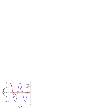
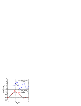
Figure 2: Response of the oscillator to the external force. Left panel – Example 1: the external force is given by (2.44). Solution (2.45) is shown for different values of $\Gamma$. Right panel – Example 2: the external force (2.47) is shown by the solid line. Dash-dotted lines depict solutions (2.49). Values of $\Gamma$ and $T_{f}$ are shown in legends.

Example 2. Interestingly, the same oscillating system, being placed in another external field, can exhibit apparently acausal reaction. To demonstrate this possibility consider the driving force acting within a finite time interval $[-T_{\rm f},+T_{\rm f}]$ and having a well defined peak occurring at $t=0$:

$$F(t)\equiv F_{2}(t)=F_{0}\cos^{2}\left(\frac{\pi\,t}{2\,T_{\rm f}}\right)\,\theta\big{(}T_{\rm f}-|t|\big{)}\,.$$ (2.47)

The oscillator response to this pulse-force is given by

$$z(t)\equiv z_{2}(t) = -\frac{F_{0}}{m}\intop_{-\infty}^{+\infty}\frac{{\rm d}\omega}{2\,\pi}\,e^{-i\,\omega\,t}\,G_{0}(\omega)\frac{\sin(\omega\,T_{\rm f})}{\omega+i\epsilon}\frac{\pi^{2}/T_{\rm f}^{2}}{(\omega+i\epsilon)^{2}-\pi^{2}/T_{\rm f}^{2}}\,.$$ (2.48)

After some manipulations the solution acquires the form

$$z_{2}(t) = \frac{F_{0}}{m\,E_{\rm R}^{2}}\big{[}\zeta(t+T_{\rm f})\,\theta(t+T_{\rm f})-\zeta(t-T_{\rm f})\,\theta(t-T_{\rm f})\big{]}\,,$$

$$\zeta(t) = \frac{1}{2}\Big{[}1-\frac{E_{\rm R}^{2}}{r_{+}r_{-}}\cos\big{(}\frac{\pi}{T_{\rm f}}\,t-\beta_{-}+\beta_{+}\big{)}+\frac{E_{\rm R}}{\omega_{\rm R}}\frac{(\pi^{2}/T^{2}_{\rm f})}{r_{+}\,r_{-}}e^{-{\textstyle\frac{1}{2}}\Gamma t}\cos\big{(}\omega_{\rm R}\,t-\beta-\beta_{-}-\beta_{+}\big{)}\Big{]}\,,$$

$$r_{\pm} = \sqrt{(\omega_{\rm R}\pm\pi/T_{\rm f})^{2}+{\textstyle\frac{1}{4}}\Gamma^{2}}\,,\quad\beta_{\pm}=\arctan\big{(}{\textstyle\frac{1}{2}}\Gamma/[\omega_{\rm R}\pm\pi/T_{\rm f}]\big{)}\,,$$ (2.49)

and the phase shift $\beta$ here is given by Eq. (2.36). The first two terms in $\zeta(t)$ are operative only for $-T_{\rm f}\leq t\leq T_{\rm f}$ and cancel out exactly for $t>T_{\rm f}$ . If the interval of the action of the force is very short, i.e. $T_{\rm f}\,E_{\rm R}\ll 1$, then for $t>T_{\rm f}$ the oscillator moves like after a single momentary kick similarly to that in Example 1, and up to the terms $\sim O(E_{\rm R}^{2}\,T_{\rm f}^{2}/\pi^{2})$ the solution (2.49) yields $z_{2}(t)\approx z_{1}(t+T_{\rm f})$ . In the opposite case, i.e. for $T_{\rm f}\,E_{\rm R}\gg 1$ and $t\in[-T_{\rm f},T_{\rm f}]$, the solution $z_{2}(t)$ oscillates around the profile of the driving force (2.47) with a small amplitude $\sim(F_{0}/mE_{\rm R}^{2})O(\pi^{2}/E_{\rm R}^{2})T_{\rm f}^{2}$,

$$(m\,E_{\rm R}^{2}/F_{0})z_{2}(t) = \frac{1}{F_{0}}F_{2}(t-\Gamma/E_{\rm R}^{2})+\frac{\pi^{2}}{2\,T_{\rm f}^{2}\,E_{\rm R}^{2}}\Big{\{}\Big{(}1-{\textstyle\frac{1}{2}}\frac{\Gamma^{2}}{E_{\rm R}^{2}}\Big{)}\,\cos\Big{(}\frac{\pi}{T_{\rm f}}\Big{[}t-\frac{\Gamma}{E_{\rm R}^{2}}\Big{]}\Big{)}$$ (2.50)

$$+ e^{-{\textstyle\frac{1}{2}}\Gamma(t+T_{\rm f})}\frac{E_{\rm R}}{\omega_{\rm R}\,}\,\cos\big{(}\omega_{\rm R}\,(t+T_{\rm f})-3\,\beta\big{)}\Big{\}}\,.$$

In the given example besides $P$ and $t_{\rm dec}^{\rm(cl)}$ the system is characterized by the initial pulse-time

$$t_{\rm pulse}=2T_{\rm f}$$ (2.51)

and by two phase time scales

$$\delta t_{\rm ph}^{(1)}=T_{\rm f}(\beta_{-}-\beta_{+})/\pi\quad\mbox{and}\quad\delta t_{\rm ph}^{(2)}=(\beta+\beta_{-}+\beta_{+})/\omega_{\rm R}\,.$$ (2.52)

The solution (2.49) is shown in Fig. 2, right panel. As we see from the lower panel, for some values of $T_{\rm f}$ and $\Gamma$ the maximum of the oscillator response may occur before the maximum of the driving force. Therefore, if for the identification of a signal we would use a detector with the threshold close to the pulse peak, such a detector would register a peak of the response of the system before the input’s peak. In Ref. [16] a similar mathematical model was used to simulate and analyze ”a causal loop paradox”, when a signal from the “future” switches off the input signal. The system with such a bizarre property has been realized experimentally [49].

Example 3. The temporal response of the system depends on characteristic frequencies of the driving force variation. For a monochromatic driving force

$$F(t)\equiv F_{3}(t)=F_{0}\,\cos(E_{p}\,t)$$ (2.53)

the solution of the equation of motion for $t>0$ is

$$z(t)=z_{3}(t)=\frac{F_{0}}{m}\,|G_{0}(E_{p})|\,\cos(E_{p}\,t-\delta(E_{p}))=\frac{(F_{0}/m)\,\cos(E_{p}\,t-\delta(E_{p}))}{\sqrt{(E_{\rm R}^{2}-E_{p}^{2})^{2}+\Gamma^{2}\,E_{p}^{2}}}\,,$$ (2.54)

where the phase shift of the oscillations compared to the oscillations of the driving force, $\delta(E_{p})$, is determined by the argument of the Green’s function

$$\delta(E_{p})=\pi+\arg G_{0}(E_{p})=\frac{i}{2}\left(\log\big{[}(E_{\rm R}^{2}-E_{p}^{2})/(E_{p}\,\Gamma)-i\big{]}-\log\big{[}(E_{\rm R}^{2}-E_{p}^{2})/(E_{p}\,\Gamma)+i\big{]}\right)\,.$$ (2.55)

The phase shift $\delta$ is determined such that $\delta(E_{p}=0)=0$. In Eq. (2.55) the logarithm is continued to the complex plane as $\log(\pm i)=\pm\pi$ so that the function $\delta(E_{p})$ is continuous at $E_{p}=E_{\rm R}$, see Fig. 3a, and in other points

$$\tan\delta(E_{p})=-E_{p}\Gamma/(E_{p}^{2}-E_{\rm R}^{2})\,.$$ (2.56)

The amplitude of the solution (2.54) has a resonance shape peaking at $E_{p}=E_{\rm R}$ with a width determined by the parameter $\Gamma$ . In contrast to Examples 1 and 2 solution (2.54) does not contain the time-scale $t_{\rm dec}^{\rm(cl)}$, since the external force does not cease with time and continuously pumps-in the energy in the system. So, two time scales, the period $P=2\pi/E_{p}$, and the phase time

$$\delta t_{\rm ph}^{(1)}=\delta(E_{p})/E_{p}$$ (2.57)

fully control the dynamics. Note that in difference with (2.14), here $E_{p}$ is the frequency rather than the particle energy.

We have seen in Example 2 that for some choices of the external force restricted in time the oscillating system can provide an apparently advanced response. The anharmonicity can produce a similar effect. For the case of small anharmonicity, $\Lambda\neq 0$, the solution (2.54) acquires a new term (an overtone)

$$z_{3\Lambda}(t)=z_{3}(t)-\frac{(F_{0}/m)^{2}\,\Lambda/(2E_{\rm R}^{2})}{\big{[}(E_{\rm R}^{2}-E_{p}^{2})^{2}+\Gamma^{2}\,E_{p}^{2}\big{]}}\Big{[}1+E_{\rm R}^{2}\,\frac{\cos\big{(}2\,[E_{p}\,t-\delta(E_{p})]-\delta(2E_{p})\big{)}}{\sqrt{(E_{\rm R}^{2}-4E_{p}^{2})^{2}+4\Gamma^{2}E_{p}^{2}}}\Big{]}\,,$$ (2.58)

which oscillates on the double frequency $2E_{p}$ and the phase is shifted with respect to the solution (2.54) by $\delta(2E_{p})$ . The Fourier transform of this solution is given by Eq. (2.37) provided $w_{0}$ is put zero. Respectively, there appears an additional phase time scale

$$\delta t_{\rm ph}^{(2)}=(\delta(E_{p})+\frac{1}{2}\delta(2E_{p}))/E_{p}$$ (2.59)

characterizing dynamics of the overtone.

In Fig. 3b we show the solution (2.58) for several frequencies $E_{p}$. If we watch for maxima in the system response $z(t)$ (shown by arrows) and compare how their occurrence is shifted in time with respect to maxima of the driving force, we observe that for most values of $E_{p}$ the overtone in (2.58) induces a small variation of the phase shift with time. However for $E_{p}\sim{\textstyle\frac{1}{2}}E_{\rm R}$ the overtone can produce an additional maximum in $z(t)$, which would appear as occurring before the actual action of the force. So the system would seem to “react” in advance.

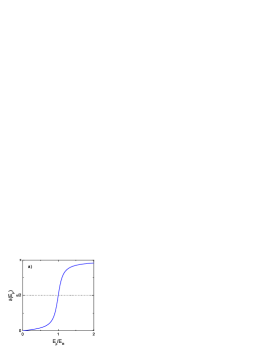
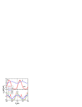
Figure 3: Panel a): Phase shift $\delta(E_{p})$ given by Eq. (2.55). Panel b): Response of the damped anharmonic oscillator to a harmonic external force (2.53) for different values of the force frequency $E_{p}$ shown by line labels in units of $E_{\rm R}$ for $\Gamma=0.2\,E_{\rm R}$ and $\Lambda=0.3\,E_{\rm R}^{4}m/F_{0}$ . Arrows show response maxima. Vertical dotted line shows maximum of the driving force.)

Example 4. In realistic cases the driving force can rarely be purely monochromatic, but is usually a superposition of modes grouped around a frequency $E_{p}$:

$$F(t)\equiv F_{4}(t)=F_{0}\intop_{-\infty}^{+\infty}{\rm d}E\,g(E-E_{p};\gamma)\,\cos(E\,t)\,,$$ (2.60)

where an envelope function $g(\epsilon;\gamma)$, $\epsilon=E-E_{p}$, is a symmetrical function of frequency deviation picked around $\epsilon=0$ with a width $\gamma$ and normalized as $\intop_{-\infty}^{+\infty}{\rm d}\epsilon\,g(\epsilon;\gamma)=1$ . The integral (2.60) can be rewritten as

$$F_{4}(t) = F_{0}\,\cos(E_{p}t)\intop_{-\infty}^{+\infty}{\rm d}\epsilon\,g(\epsilon;\gamma)\,\cos(\epsilon\,t)=\mathcal{A}_{F}(\gamma t)\cos(E_{p}t)\,,$$ (2.61)

that allows us to identify $E_{p}$ as the carrier frequency and $\mathcal{A}_{F}(\gamma t)$, as the amplitude modulation depending on dimension-less variable $\gamma t$.

For $\Lambda=0$, the particle motion is described by the function

$$z_{4}(t) = -\intop_{-\infty}^{+\infty}\frac{{\rm d}\omega}{2\,\pi}e^{-i\,\omega\,t}G_{0}(\omega)\,\frac{1}{m}\,F(\omega)=-\frac{F_{0}}{m}\intop_{-\infty}^{+\infty}\frac{{\rm d}\omega}{2\,\pi}e^{-i\,\omega\,t}G_{0}(\omega)\,\pi\big{[}g(\omega+E_{p};\gamma)+g(\omega-E_{p};\gamma)\big{]}$$ (2.62)

$$= -\frac{F_{0}}{m}\Re\intop_{-\infty}^{+\infty}{\rm d}\epsilon e^{-i\,(E_{p}+\epsilon)\,t}G_{0}(E_{p}+\epsilon)\,g(\epsilon;\gamma)\,.$$

The last integral can be formally written as

$$m\,z_{4}(t) = |G_{0}(E_{p})|\Re e^{-i(E_{p}\,t-\delta(E_{p}))}e^{-{\textstyle\frac{1}{2}}\partial^{2}_{E}\log G_{0}(E_{p})\,\partial_{t}^{2}+O(\partial_{t}^{3})}\,\mathcal{A}_{F}\big{(}\gamma(t+i\,\partial_{E}\log G_{0}(E_{p}))\big{)}.$$ (2.63)

Here $O(\partial^{3}_{t})$ represents time derivatives of the third order and higher. We used the relation $\log G_{0}(E)=\log|G_{0}(E)|+i\,\delta(E)-i\,\pi$, where $\delta(E)$ is defined as in Eq. (2.55), but now as function of $E$ rather than $E_{p}$. The first-order derivatives generate the shift of the argument of the amplitude modulation via the relation $\exp(a\,\partial_{t})\,\mathcal{A}_{F}(t)=\mathcal{A}_{F}(t+a)$ . Note that the time shift of $\mathcal{A}_{F}(t)$ involves formally the ”imaginary time”. As we will see later in Sect. 3, the same concept appears also in quantum mechanics.

To proceed further with Eq. (2.63) one may assume that the function $\mathcal{A}_{F}(t)$ varies weakly with time so that the second and higher time derivatives can be neglected. In terms of the envelop function, this means that $g(\epsilon)$ is a very sharp function falling rapidly off for $\epsilon\gtrsim\gamma$ while $\gamma\ll\Gamma$. A typical time, on which the function $\mathcal{A}_{F}(t)$ fades away, can be estimated as

$$t^{\gamma,(\rm cl)}_{\rm dec}=1/\gamma,$$ (2.64)

If, additionally, the oscillator system has a high quality factor, i.e., $\Gamma\ll E_{\rm R}$ and $|\partial_{E}\log|G_{0}(E_{p})||\ll\delta^{\prime}(E_{p})$, that is correct for $E_{p}$ very near $E_{\rm R}$, we arrive at the expression

$$m\,z_{4}(t)=\mathcal{A}_{F}\left(t-\delta^{\prime}(E_{p}))\right)\,|G_{0}(E_{p})|\,\cos(E_{p}\,t-\delta(E_{p}))\,.$$ (2.65)

We see that in this approximation there are five time scales determining the response of the system. The oscillations are characterized by the period $P=2\pi/E_{p}$ and damping time $t_{\rm dec}^{\rm(cl)}=2/\Gamma$. Moreover, the envelope function is damping on the time scale $t^{\gamma,(\rm cl)}_{\rm dec}$. Additionally, there are two delay time scales: Oscillations of the carrier wave are delayed by the phase time $\delta t_{\rm ph}^{\rm(cl)}(E_{p})={\delta(E_{p})}/{E_{p}}\,,$ see (2.57), whereas the amplitude modulation $\mathcal{A}_{F}$ is delayed by the group time

$$t_{\rm gr}^{\rm(cl)}(E_{p})=\frac{\partial\delta(E_{p})}{\partial E_{p}}=-\frac{E_{R}^{2}+E_{p}^{2}}{E_{p}}\,\Im G_{0}(E_{p})\,.$$ (2.66)

This time shift appears because the system responses slightly differently to various frequency modes contributing to the force envelop (2.60).

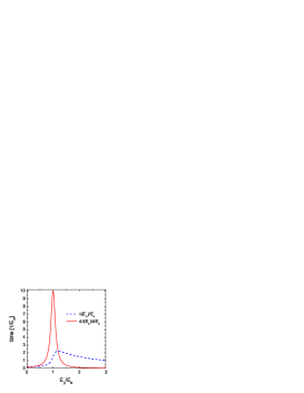
Figure 4: The phase and group time delays given by Eqs. (2.57) and (2.66), respectively, calculated for $\Gamma=0.2E_{\rm R}$. The horizontal line shows the decay width $t_{\rm dec}^{(cl)}$.

The group and phase times are shown in Fig. 4. The group time is much more rapidly varying function of the external frequency $E_{p}$ and is strongly peaked at $E_{p}\sim E_{\rm R}$ . Close to the resonance the group time can be written as

$$t_{\rm gr}^{(1)}(E_{p})\approx\frac{\Gamma/2}{(E_{p}-E_{\rm R})^{2}+{\textstyle\frac{1}{4}}\Gamma^{2}}={\textstyle\frac{1}{2}}A_{1}(E_{p})>0\,.$$ (2.67)

For $\Lambda\neq 0$ there also appear another resonances in the system response, see Eq. (2.58). In the linear in $\Lambda$ approximation the resonance with $E_{p}\simeq{\textstyle\frac{1}{2}}E_{\rm R}$ is excited. Close to this resonance the group time is

$$t^{(2)}_{\rm gr}(E_{p})\approx\frac{\Gamma/4}{(E_{p}-E_{\rm R}/2)^{2}+{\textstyle\frac{1}{4}}(\Gamma/2)^{4}}={\textstyle\frac{1}{2}}A_{2}(E_{p})>0\,$$ (2.68)

with a maximum at $E_{p}=E_{\rm R}/2$. The width of the peak is $\Gamma/4$. Note that for both modes the functions $A_{1,2}(E_{p})$ satisfy the sum-rule

$$\int_{-\infty}^{\infty}A_{1,2}(E){\rm d}E/(2\pi)=1\,,\quad\mbox{or}\quad\int_{-\infty}^{\infty}t_{\rm gr}^{(1,2)}(E){\rm d}E/\pi=1\,.$$ (2.69)

The energy-time sum-rules demonstrate relation of the group times to the density of states, i.e. re-grouping of the number of degrees of freedom.

The time-difference

$$\delta t_{\rm f}^{\gamma}=t^{(i)}_{\rm gr}-t^{\gamma,(\rm cl)}_{\rm dec},$$ (2.70)

we call it forward time delay/advance, demonstrates are the groups of waves delayed on the scale of degrading of the envelop function. As is seen from Fig. 4, in the near resonance region $\delta t_{\rm f}^{\gamma}>0$, whereas in the off-resonance region $\delta t_{\rm f}^{\gamma}<0$. As we shall see in Sect. 3, an important case is when $\gamma\sim\Gamma$.

To study corrections to Eq. (2.65) due to the second-order derivatives in Eq. (2.63) we turn back to the case $\Lambda=0$ and take the Gaussian envelope function $g_{\rm Gauss}(\epsilon)$ and the corresponding amplitude modulation $\mathcal{A}_{F,{\rm Gauss}}(\gamma t)$, such that

$$g_{\rm Gauss}(\epsilon;\gamma)=\frac{\exp(-\epsilon^{2}/2\gamma^{2})}{\sqrt{2\,\pi\,\gamma^{2}}}\,,\quad\mathcal{A}_{F,{\rm Gauss}}(t;\gamma)=F_{0}\exp(-\gamma^{2}t^{2}/2)\,.$$ (2.71)

Then, using the identity

$$e^{a\,\partial^{2}_{t}}\,e^{-\gamma^{2}t^{2}/2}\equiv\sum_{n=0}^{\infty}\frac{a^{n}}{n!}\,\partial_{t}^{2\,n}e^{-\gamma^{2}t^{2}/2}=\frac{e^{-\gamma^{2}t^{2}/2(1+2\,a\,\gamma^{2})}}{\sqrt{1+2\,a\,\gamma^{2}}}\,,$$ (2.72)

we obtain the response of the system to the Gaussian force in the form

$$z_{4{\rm Gauss}}(t) = \frac{F_{0}}{m}|G_{0}(E_{p})|\Re\,\frac{e^{-i\,(E_{p}\,t-\delta(E_{p}))}}{\sqrt{1-\gamma^{2}\partial^{2}_{E}\log G_{0}(E_{p})}}\exp\left[-\gamma^{2}\frac{\big{(}t+i\partial_{E}\log G_{0}(E_{p})\big{)}^{2}}{2\big{(}1-\gamma^{2}\partial^{2}_{E}\log G_{0}(E_{p})\big{)}}\right]\,.$$ (2.73)

The derivatives of the Green’s function can be conveniently expressed through the Green’s function as

$$\partial_{E}\log G_{0}(E)=i\,\delta^{\prime}(E)+\partial_{E}\log|G_{0}(E)|=-(2\,E+i\,\Gamma)\,G_{0}(E)\,,$$

$$\partial^{2}_{E}\log G_{0}(E)=i\,\delta^{\prime\prime}(E)+\partial_{E}^{2}\log|G_{0}(E)|=2\,G_{0}(E)+(4\,E_{\rm R}^{2}-\Gamma^{2})\,G_{0}^{2}(E)\,.$$ (2.74)

After some algebra we can cast this expression in the form similar to Eq. (2.65) with the amplitude modulation (2.71):

$$m\,z_{4{\rm Gauss}}(t)=\mathcal{A}_{F,{\rm Gauss}}\big{(}t-\tilde{t}_{\rm gr}^{\rm(cl)};\tilde{\gamma}\big{)}\,C_{\gamma}\,|G_{0}(E_{p})|\,\cos(\widetilde{E}_{p}(t)\,t-\tilde{\delta}(E_{p}))\,,$$ (2.75)

where, however, we have to redefine parameters of both the carrier wave and the amplitude modulation function. The width of the Gaussian packet is determined from expression

$$\tilde{\gamma}^{2}=\gamma^{2}\frac{1-\gamma^{2}\,\partial_{E}^{2}\log|G_{0}(E_{p})|}{|1-\gamma^{2}\partial_{E}^{2}\log G_{0}(E_{p})|^{2}}\,,$$ (2.76)

and the amplitude modulation is delayed by the group time

$$\tilde{t}_{\rm gr}^{\rm(cl)}=\delta^{\prime}(E_{p})+\partial_{E}\log|G_{0}(E_{p})|\,\frac{\gamma^{2}\delta^{\prime\prime}(E_{p})}{1-\gamma^{2}\partial_{E}^{2}\log|G_{0}(E_{p})|}\,.$$ (2.77)

An interesting effect is that the frequency of the carrier wave is changed and even becomes time dependent,

$$\widetilde{E}_{p}(t)=E_{p}+\tilde{\gamma}^{2}\,\Big{[}\partial_{E}\log|G_{0}(E_{p})|+({\textstyle\frac{1}{2}}t-\delta^{\prime}(E_{p}))\frac{\gamma^{2}\delta^{\prime\prime}(E_{p})}{1-\gamma^{2}\partial_{E}^{2}\log|G_{0}(E_{p})|}\Big{]}\,,$$ (2.78)

and the phase shift is given by

$$\tilde{\delta} = \delta(E_{p})+{\textstyle\frac{1}{2}}\arctan\Big{(}\frac{\gamma^{2}\,\delta^{\prime\prime}(E_{p})}{1-\gamma^{2}\partial^{2}_{E}\log|G_{0}(E_{p})|}\Big{)}$$ (2.79)

$$+ \tilde{\gamma}^{2}\,\Big{[}\delta^{\prime}(E_{p})\,\partial_{E}\log|G_{0}(E_{p})|+{\textstyle\frac{1}{2}}\big{(}\big{[}\partial_{E}\log|G_{0}(E_{p})\big{]}^{2}-\big{[}\delta^{\prime}(E_{p})\big{]}^{2}\big{)}\frac{\gamma^{2}\delta^{\prime\prime}(E_{p})}{1-\gamma^{2}\partial_{E}^{2}\log|G_{0}(E_{p})|}\Big{]}\,.$$

The amplitude of the system response is modulated by the factor

$$C_{\gamma}=\exp\Big{[}{\textstyle\frac{1}{2}}\gamma^{2}\frac{\big{[}\partial_{E}\log|G_{0}(E_{p})|\big{]}^{2}}{(1-\gamma^{2}\partial_{E}^{2}\log|G_{0}(E_{p})|)^{2}}\Big{]}\bigg{/}{|1-\gamma^{2}\partial_{E}^{2}\log G_{0}(E_{p})|}\,.$$ (2.80)

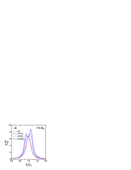
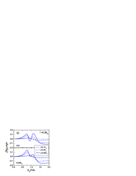
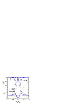
Figure 5: Parameters of the system response (2.73) to the modulated periodic external force (2.61) with the Gaussian envelop (2.71) calculated including the second-order derivatives for several values of the envelop width $\gamma$ as functions of the force oscillation frequency $E_{p}$. The damping parameter of the system is $\Gamma=0.3\,E_{\rm R}$ . Panel a): Time shift of the amplitude modulation (2.77) for various values of $\gamma$. The dotted line shows the time shift (2.66) entering in the leading-order expression (2.65) involving the first-order derivatives only. Panel b): Relative deviation of the oscillation quasi-period $\widetilde{P}(t)=2\pi/\widetilde{E}_{p}(t)$, see Eq. (2.78), from the force oscillation period $P=2\pi/E_{p}$ for two moments of time $t=0$ and $t=3/E_{\rm R}$ . Panel c): Modification of the packet width $(\tilde{\gamma}/\gamma)^{2}$ given by Eq. (2.76) and the amplitude scaling factor $C_{\gamma}$ given by Eq. (2.80) .

Keeping terms quadratic in $\gamma$ we find the corrected group and phase times

$$\tilde{t}_{\rm gr}^{\rm(cl)}\simeq\delta^{\prime}(E_{p})+\gamma^{2}\,\partial_{E}\log|G_{0}(E_{p})|\,\delta^{\prime\prime}(E_{p})+O(\gamma^{4})\,,$$ (2.82)

$$E_{p}\delta\tilde{t\,}_{\rm ph}^{\rm(cl)}\simeq\delta(E_{p})+\gamma^{2}\,\Big{(}{\textstyle\frac{1}{2}}\delta^{\prime\prime}(E_{p})+\partial_{E}\log|G_{0}(E_{p})|\,\big{(}\delta^{\prime}(E_{p})\,-\delta(E_{p})/E_{p}\big{)}\Big{)}+O(\gamma^{4})\,.$$

The importance of various correction terms depends on how close the carrier frequency $E_{p}$ is to the resonance frequency $E_{\rm R}$. Assuming that the oscillator has a high quality factor $\Gamma\ll E_{\rm R}$, we can distinguish three different regimes: $(i)$ very near to the resonance, $|E_{p}-E_{\rm R}|\lesssim\Gamma^{2}/E_{\rm R}$, $(ii)$ an intermediate regime, $\Gamma^{2}/E_{\rm R}\ll|E_{p}-E_{\rm R}|\lesssim\Gamma$, and $(iii)$ far from the resonance $\Gamma\ll|E_{p}-E_{\rm R}|$ . In the regime $(i)$ corrections in (2.82), (2.82) are respectively of the order of $O(\gamma^{2}/E_{\rm R}^{2})$ and $O(\gamma^{2}/E_{\rm R}\Gamma)$. In the regime $(ii)$ correction terms are of the order of $O(\gamma^{2}/\Gamma^{2})$. In the regime $(iii)$ corrections are respectively of the order of $O(\gamma^{2}/E_{\rm R}^{2})$ and $O(\gamma^{2}\Gamma/E_{\rm R}^{3})$ at most.

To illustrate the applicability range of the leading-order expression (2.65) and the size of the corrections in Eq. (2.75) we plot in Fig. 5 the quantities (2.76), (2.77), (2.78), (2.80) versus the force oscillation frequency $E_{p}$ for various values of the envelop width $\gamma$ and $\Gamma=0.3\,E_{\rm R}$ . We see that, as argued before, the corrections are small for $E_{p}$ far from the resonance frequency $E_{\rm R}$ and right at the resonance. The corrections are maximal for $E_{p}\sim E_{\rm R}\pm\Gamma$ . Remarkably, at these frequencies the system response could become significantly broader (i.e. it lingers longer in time) than the driving force, $\tilde{\gamma}<\gamma$. Figure 5 shows also that Eq. (2.65) can be used only for $\gamma/\Gamma\ll 0.3$. The expression (2.75) is applicable for $\gamma/\Gamma\lesssim 0.5$ and $\Gamma/E_{\rm R}\lesssim 0.3$ at the 30% accuracy level. For higher values of $\gamma$ the corrections become too large and further terms in expansion (2.63) have to be taken into account.

In Fig. 6 we depict the response of the system to the force (2.61) with the ’broad’ Gaussian envelop (2.71), $\gamma=\Gamma$, as it follows from numerical evaluation of the integral (2.62). We clearly see that when $E_{p}$ approaches the interval $E_{\rm R}\pm\Gamma$ not only the amplitude of the system response grows, but also the response lasts much longer than the force acts. Thus we demonstrated peculiarities of the effect of a smearing of the wave packet in classical mechanics.

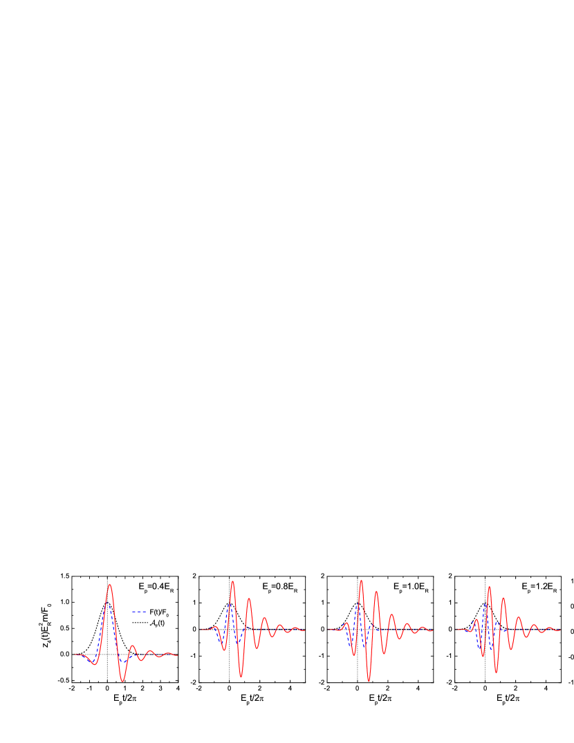
Figure 6: Solid lines: response (2.62) of the oscillatory system to the modulated periodic external force (2.61) with the Gaussian envelop (2.71) calculated for $\gamma=\Gamma=0.3E_{\rm R}$ and various values of the force frequency $E_{p}$. Dashed lines show the external force (2.61) and dotted lines depict the envelop function (2.71).

2.1.3 Simple 3D-example. Scattering of particles on hard spheres

Consider a simplest case when a beam of (point-like) particles falls onto a hard sphere of a radius $R$, cf. [4]. The particles scatter at different angles $\theta$, $\sin(\theta/2)=\sqrt{1-b^{2}/R^{2}}$  depending on the impact parameter $b$. The arrival time of the scattered particle to the detector decreases with an increase of the size of the sphere. The time advance for the particle scattered on the sphere surface compared to that it would scatter on the center in the same $\theta$ direction is

$$\delta t_{\rm W}^{\rm(cl)}=-2\frac{\Delta l}{v}=-\frac{2\,R}{v}\sin\frac{\theta}{2}\geq-\frac{2\,R}{v}\,,$$ (2.83)

see Fig. 7. In the given example $\delta t_{\rm soj}^{\rm(cl)}=\delta t_{\rm W}^{\rm(cl)}$, as they were introduced above, see Eqs. (2.15), (2.17). As is seen from (2.17), for the repulsive potential $V=a/(r-b)^{\alpha}$, $r>r_{0}=r(v_{r}=0)$, $a>0$, $\alpha>0$, as in case of the scattering on the hard sphere, there appears a time advancement, provided $r_{0}$ being very close to $b$. However the value of the Wigner time advancement is limited.

As we shall see below, the relevant quantity related to the advance/delay of the scattered wave, the scattering advance/delay time, is the half of the Wigner advance/delay time. In the given hard sphere example thus introduced quantity,

$$\delta t_{\rm s}^{\rm(cl)}={\textstyle\frac{1}{2}}\delta t_{\rm W}^{\rm(cl)}\,,$$ (2.84)

is the difference of time, when the particle touches the sphere surface, and the time, when the particle freely reaches the center of the sphere. The advance $\delta t_{\rm s}^{\rm(cl)}$ is limited by the value $-R/v$.

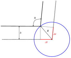
Figure 7: Particle scattering at angle $\theta$ off the hard sphere of radius $R$

Note that the averaged advance time for all scattered particles incident on the sphere at various impact parameters $0\leq b\leq R$ is

$$\langle\delta t_{\rm W}^{\rm(cl)}\rangle=\intop_{0}^{R}\delta t_{\rm W}^{\rm(cl)}\,\frac{2\pi\,b{\rm d}b}{\pi R^{2}}=-\frac{4}{v\,R^{2}}\intop_{0}^{R}\sqrt{R^{2}-b^{2}}\,b{\rm d}b=-\frac{4}{3}\frac{R}{v}\,.$$ (2.85)

From the above analysis we are able also to conclude that the collision term in the kinetic equation describing behavior of a non-equilibrium gas of hard spheres should incorporate mentioned non-local time advancement effects.

2.2 Time shifts in classical electrodynamics

2.2.1 Dipole radiation of charged oscillator

Let us consider the same damped oscillatory system, as in the previous subsections, assuming now that the particle is charged and oscillates in the $z$ direction near the point $z=0$ under the action of an incident electromagnetic wave propagating in the $x$ direction with the electric field polarized along the $z$ axis:

$$\vec{\mathcal{E}}_{\rm in}(t,\vec{r}\,)=\mathcal{E}_{0}\,\vec{e}_{z}\,\cos\big{(}\vec{p}\,\vec{r}-E_{p}\,t\big{)}\,,\quad\vec{\mathcal{H}}_{\rm in}(t,\vec{r}\,)=[\vec{e}_{x}\times\vec{\mathcal{E}}_{\rm in}]\,,\quad\vec{p}=p\,\vec{e}_{x}\,.$$ (2.86)

Here $\vec{e}_{x(yz)}$ denotes the unit vector along $x(yz)$ direction, $E_{p}=c\,p$ and $c$ is the speed of light. We assume that the field weakly changes over the range of particle oscillations. Then the force acting on the charge is $\vec{F}(t)\approx\mathcal{E}_{0}\,\vec{e}_{z}\cos(E_{p}\,t)$ and the oscillations are described by Eq. (2.54) of the previous section. The electric dipole moment induced in the system by the incident wave is given by

$$\vec{d}(t)=ez(t)=\frac{e^{2}\,\mathcal{E}_{0}}{m}\frac{\cos\big{(}E_{p}\,t-\delta(E_{p})\big{)}}{\sqrt{(E_{\rm R}^{2}-E_{p}^{2})^{2}+\Gamma_{\rm tot}^{2}\,E_{p}^{2}}}\,\vec{e}_{z}\,,\quad\Gamma_{\rm tot}=\Gamma+\Gamma_{\rm rad}\,,$$ (2.87)

$\Gamma_{\rm tot}$ is the total width of the oscillator. The oscillating dipole emits electromagnetic waves. Therefore, there is a dissipative process due to the radiation friction force, $\Gamma_{\rm rad}=2e^{2}\,E_{p}^{2}/(3\,m\,c^{3})$  for $E_{p}\lesssim E_{\rm R}$, which we consider. The additional damping effects included in $\Gamma$ are, e.g., due to atomic collisions, provided the charged particle oscillates in medium. The formulated model is the well-known Lorentz model for vibrations of an electron in an atom. An ensemble of such oscillators resembles a dispersive medium.

Far from the dipole in the so-called wave zone $|d_{\rm max}/e|\ll\lambda\ll r$, where $\lambda=2\pi/p$ is the radiation wave-length and $|d_{\rm max}/e|$ is the amplitude of the oscillations, the outgoing waves of electric and magnetic fields are given by [50]

$$\vec{\mathcal{E}}_{\rm out}(t,\vec{r})=\frac{1}{r\,c^{2}}[\vec{n}_{r}\times[\vec{n}_{r}\times\ddot{\vec{d}}(t-r/c)]]\,,\quad\vec{\mathcal{H}}_{\rm out}(t,\vec{r})=[\vec{n}_{r}\times\vec{\mathcal{E}}_{\rm out}(t,\vec{r})]=\frac{1}{r\,c^{2}}[\ddot{\vec{d}}(t-r/c)\times\vec{n}_{r}]$$ (2.88)

with $\vec{n}_{r}=\vec{r}/|\vec{r}\,|$ . The time shift $t-r/c$ arises due to finiteness of the speed of light. The scattered electric field is polarized along a meridian, $\vec{\mathcal{E}}_{\rm out}\parallel\vec{e}_{\theta}$ .

The differential cross section for the scattering process can be defined as the ratio of the time-averaged intensity of the induced radiation ${\rm d}\bar{I}$, passing through a sufficiently large sphere of radius $R_{0}$, to the time-averaged energy flux of the incident wave falling on the oscillator, see §78 in [50],

$$d\sigma=\frac{1}{\overline{\vec{S}_{\rm in}}}{\rm d}\bar{I}\,,\quad{\rm d}I=\vec{S}_{\rm out}{\rm d}\vec{s}_{r}\,.\quad\vec{S}_{\rm in(out)}=\frac{c}{4\pi}\big{[}\vec{E}_{\rm in(out)}\times\vec{H}_{\rm in(out)}\big{]}\,.$$

Here the line over a symbol means a time average over the oscillation period and ${\rm d}\vec{s}_{r}$ is element of the surface oriented in the direction $\vec{n}_{r}$ . With the help of Eqs. (2.86) and (2.88) we find

$$\vec{S}_{\rm in}=\frac{c}{4\pi}\,\mathcal{E}^{2}_{0}\,\cos^{2}(E_{p}\,t)\,\vec{e}_{x}\,,\quad{\rm d}I=(\vec{S}_{\rm out}\vec{n}_{r})R_{0}^{2}{\rm d}\Omega=\frac{1}{4\pi\,c^{3}}\big{[}\ddot{\vec{d}}(t-R_{0}/c)\times\vec{n}_{r}\big{]}^{2}\,{\rm d}\Omega\,.$$ (2.89)

Using Eq. (2.87) and performing the averaging over the time we obtain [50]

$$\frac{{\rm d}\sigma}{{\rm d}\Omega}=\Big{(}\frac{e^{2}}{m\,c^{2}}\Big{)}^{2}\frac{E_{p}^{4}}{(E_{\rm R}^{2}-E_{p}^{2})^{2}+\Gamma_{\rm tot}^{2}\,E_{p}^{2}}[\vec{e}_{z}\times\vec{n}_{r}]^{2}\,.$$ (2.90)

We chose the spherical coordinate system so that the polar angle corresponds to the scattering angle $\theta$ — the angle between the propagation directions of incoming and outgoing waves, $\cos\theta=(\vec{n}_{r}\,\vec{p})/p$. Then the vector product in (2.90) can be written as $[\vec{e}_{z}\times\vec{n}_{r}]^{2}=\cos^{2}\theta+\sin^{2}\theta\,\sin^{2}\phi$ . Thus the cross section depends on the azimuthal angle that corresponds to a scattering of photons with different magnetic quantum numbers: $[\vec{e}_{z}\times\vec{n}_{r}]^{2}=\frac{4\pi}{3}|Y_{1,0}(\theta,\phi)+(Y_{1,+1}(\theta,\phi)+Y_{1,-1}(\theta,\phi))/\sqrt{2}|^{2}$, where $Y_{l,m}(\theta,\phi)$ are the spherical functions. The magnetic number dependence appears because we have confined the oscillator motion to one dimension. For a spherically symmetric scattering this dependence would be averaged out.

The differential cross section can now be written as

$$\frac{{\rm d}\sigma}{{\rm d}\Omega} = \frac{\pi}{p^{2}}\frac{3\,\,\Gamma_{\rm tot}^{2}E_{p}^{2}}{(E_{\rm R}^{2}-E_{p}^{2})^{2}+\Gamma_{\rm tot}^{2}\,E_{p}^{2}}B_{\rm rad}^{2}\Big{|}Y_{10}(\theta,\phi)+\frac{1}{\sqrt{2}}\big{(}Y_{1-1}(\theta,\phi)+Y_{1-1}(\theta,\phi)\big{)}\Big{|}^{2}\,,$$ (2.91)

where we introduced the branching ratio $B_{\rm rad}=\Gamma_{\rm rad}/\Gamma_{\rm tot}$. One can introduce the scattering amplitude as

$$\frac{{\rm d}\sigma}{{\rm d}\Omega} = \big{|}f(\theta,\phi)\big{|}^{2}\,,\ \quad f(\theta,\phi)=\sum_{l=0}^{\infty}\sqrt{2\,l+1}\,\sqrt{4\pi}\sum_{m=-l}^{l}{f}_{l,m}\,Y_{l,m}(\theta,\phi)\,.$$ (2.92)

For the spherically symmetrical scattering the amplitude would be

$$f(\theta)=\sum_{l=0}^{\infty}(2\,l+1){f}_{l}\,P_{l}(\cos\theta)\,.$$ (2.93)

Here $P_{l}(\cos\theta)$ are Legendre polinomials normalized as [51]: $\int_{-1}^{1}P_{l}^{2}(x)dx=2/(2l+1)$.

In our case the scattering amplitude has only terms with $l=1$ and $\sqrt{2}\,{f}_{1,\pm 1}={f}_{1,0}\equiv{f}_{1}$ with

$$2p{f}_{1}=\frac{B_{\rm rad}\,\Gamma_{\rm tot}\,E_{p}}{E_{\rm R}^{2}-E_{p}^{2}-i\,\Gamma_{\rm tot}\,E_{p}}=\frac{B_{\rm rad}}{\cot\delta(E_{p})-i}=B_{\rm rad}\sin\delta(E)e^{i\delta(E_{p})}.$$ (2.94)

The phase of the scattered waves $\delta(E_{p})$ is defined as in Eqs. (2.55), and (2.56) but now with $\Gamma_{\rm tot}$ instead of $\Gamma$, i.e. $\tan\delta(E_{p})=-\Gamma_{\rm tot}E_{p}/(E_{p}^{2}-E_{\rm R}^{2})$ .

After integration over the scattering angle the total cross section can be cast in the standard spin-averaged Breit-Wigner resonance form (see page 374 in Ref. [52])

$$\sigma = {2(2l+1)}{4\pi}|{f}_{l}|^{2}=\frac{3}{2}\,\frac{4\pi}{p^{2}}\frac{\Gamma_{\rm tot}^{2}\,E_{p}^{2}}{(E_{\rm R}^{2}-E_{p}^{2})^{2}+\Gamma_{\rm tot}^{2}\,E_{p}^{2}}B_{\rm rad}^{2}\,.$$ (2.95)

Here the statistical factors correspond to the angular momentum, $l=1$ in our case.

From the structure of Eq. (2.87) we see that the concepts of the phase and group time delays (2.57) and (2.66) are also applicable to electromagnetic waves, if we deal with not a monochromatic wave but a wave packet instead. If the incoming wave were like $|\vec{\mathcal{E}}_{\rm in}|=\mathcal{E}_{0}\,f_{\mathcal{E}}(\vec{p}\vec{r}-E_{p}\,t)\cos\big{(}\vec{p}\vec{r}-E_{p}\,t\big{)}$ with some function $f_{\mathcal{E}}(x)$ integrable in the interval $(-\infty,+\infty)$, then the outgoing wave would be $|\vec{\mathcal{E}}_{\rm out}|\propto\mathcal{E}_{0}\,f_{\mathcal{E}}(t-\delta t_{\rm s}^{\rm(cl)}-r/c)\cos\big{(}p\,r-E_{p}\,[t-\delta(E_{p})]\big{)}$ . The propagation of the scattered wave packet is delayed by the group time (2.66), see also (2.67), (2.68),

$$t_{\rm s}^{\rm(cl)}=\frac{\partial\delta}{\partial E_{p}}\approx\frac{A}{2}=\frac{\Gamma_{\rm tot}/2}{(E_{p}-E_{\rm R})^{2}+\Gamma^{2}_{\rm tot}/4}>0,$$ (2.96)

which here in three dimensional case has meaning of the scattering delay time, being twice as small compared to the Wigner delay time introduced above, see Eq. (2.21). Here we performed expansion in frequencies close to the resonance $E_{p}\sim E_{\rm R}$ . With $t_{\rm s}^{\rm(cl)}$ from Eq. (2.96), the scattered wave appears with a delay compared to the condition $t-r/c\geq 0$. Thus causality requires that the scattered wave arises for $t-t_{\rm s}^{\rm(cl)}-r/c\geq 0$.

2.2.2 Scattering of light on hard spheres

For the scattering of light on a hard sphere of radius $R$, the causality condition can be formulated as [4, 2]: if the incident wave propagating along $z$ direction vanishes for $t<z/c$, the scattered wave in the direction $\theta$ must vanish for $t<\big{(}r-2\,R\sin(\theta/2)\big{)}/c$. The quantity $2R\sin(\theta/2)$ is the difference in the paths of the light scattered at angle $\theta$ on the sphere surface and on the sphere center (2.83).

The scattering process (when the beam just touches the sphere) proceeds with twice shorter advance compared the time $R/c$ which the light would pass to the center of the sphere, cf. (2.83). Correspondingly, the advancement in the scattering time, $\delta t_{\rm s}^{\rm(cl)}$, proves to be twice as small compared to the advancement in the Wigner time, $\delta t_{\rm W}^{\rm(cl)}$.

3 Time shifts in non-relativistic quantum mechanics: 1D-scattering

The problem of how to quantify a duration of quantum mechanical processes has a long and vivid history. It started with a statement of Wolfgang Pauli [53] that in the framework of traditional non-relativistic quantum mechanics it is impossible to introduce a hermitian (self-adjoint) linear operator of time, which is canonically conjugate to the Hamiltonian. The reason for this is that for most of the systems of physical interest the Hamiltonian is bounded from below.  Later on a variety of ’time-like’ observables were introduced tailored for each particular system. For a comprehensive review of the history of this question we address the reader to the Introduction in Ref. [10]. Various inter-related definitions of time appeared, for instance, in considerations of the following questions: How long does the quantum transition last (quantum jump duration) [55, 56]? What are interpretations of time-energy uncertainty relations [57]? How one can quantify a time of flight or a time of arrival of a particle to a given point [58, 59]? How long does it take for a particle to tunnel through a barrier [60, 13, 61, 62, 63, 8]? What is a life time of a resonance [3, 64, 65, 5, 20]? What is the duration of particle collision [1, 66, 3, 2]?

Without any pretense to address all these issues, in this section we would like to introduce the basic concepts related to the temporal characteristics of typical quantum mechanical processes, such as tunneling, scattering, and decay.

3.1 Stationary problem

We begin with a one-dimensional quantum-mechanical system, described by the Hamiltonian $\hat{H}=\hat{H}_{0}+\hat{U}$ consisting of the free motion Hamiltonian $\hat{H}_{0}=-\frac{\hbar^{2}}{2\,m}\frac{\partial^{2}}{\partial z^{2}}$ for a particle with mass $m$ and of an arbitrary potential $\hat{U}=U(z)\geq 0$, which is assumed to be localized within the interval $-L/2<z<L/2$ and vanishing elsewhere outside. This Hamiltonian has a continuous spectrum $0<E<+\infty$ and the complete set of eigenfunctions $\psi(z;E)$ obeying the equation $\hat{H}\psi(z;E)=E\,\psi(z;E)$. We will consider the wave functions satisfying the asymptotic conditions for the standard scattering problem 

$$\psi_{1}(z;E) = \left\{\begin{array}[]{lll}e^{i\,k\,z/\hbar}+R_{1}(E)\,e^{-i\,k\,z/\hbar}&,&z<-{\textstyle\frac{1}{2}}L,\\ \psi_{U,1}(z;E)&,&-{\textstyle\frac{1}{2}}L\leq z\leq{\textstyle\frac{1}{2}}L\\ T_{1}(E)\,e^{+i\,k\,z/\hbar}&,&{\textstyle\frac{1}{2}}L<z,\end{array}\right.\,,$$ (3.100)

$$\psi_{2}(z;E) = \left\{\begin{array}[]{lll}T_{2}(E)\,e^{-i\,k\,z/\hbar}&,&z<-{\textstyle\frac{1}{2}}L,\\ \psi_{U,2}(z;E)&,&-{\textstyle\frac{1}{2}}L\leq z\leq{\textstyle\frac{1}{2}}L,\\ R_{2}(E)\,e^{+i\,k\,z/\hbar}+e^{-i\,k\,z/\hbar}&,&{\textstyle\frac{1}{2}}L<z,\end{array}\right.$$ (3.104)

with $k=\sqrt{2\,m\,E}>0$ . The wave functions $\psi_{1}$ and $\psi_{2}$ describe the physical situation when a particle beam from the left or from the right, respectively, incident on the potential becomes split into a reflected part with the amplitude $R_{1,2}$ and a transmitted part with the amplitude $T_{1,2}$. The wave functions are normalized to the unit incident amplitude. Then the quantities $|R_{1,2}|^{2}$ and $|T_{1,2}|^{2}$ have the meaning of the reflection and transmission probabilities, respectively, and $|R_{1,2}|^{2}+|T_{1,2}|^{2}=1$ . For any given wave function $\Psi$ the current is calculated standardly

$$\mathcal{J}[\Psi]=\frac{i\hbar}{2\,m}\left(\Psi\nabla_{z}\Psi^{*}-\Psi^{*}\nabla_{z}\Psi\right)\,.$$ (3.105)

Thus, for the wave function $\psi_{1}$ we can define three currents: the incident current $j_{\rm I}=\mathcal{J}[\exp(i\,k\,z/\hbar)]=\frac{k}{m}$, the transmitted current $j_{\rm T}=\mathcal{J}[\psi_{1}(z>{\textstyle\frac{1}{2}}L)]=|T_{1}(E)|^{2}j_{\rm I}$ and the reflected current $j_{\rm R}=\mathcal{J}[\psi_{1}(z<-{\textstyle\frac{1}{2}}L)]-j_{\rm I}=-|R_{1}(E)|^{2}j_{\rm I}$. The current conservation is fulfilled and $j_{\rm I}=j_{\rm T}-j_{\rm R}$ . Here, it is important to notice that in the region of the potential there exists an ”internal” current $j_{\rm int}=\mathcal{J}[\psi_{U,1}(z)]$. In case of the classically allowed motion above the barrier $j_{\rm int}=j_{\rm T}$ is determined by the sum of the currents of the forward-going wave and of the backward-going wave, whereas in the region under the barrier $j_{\rm int}$ is determined by the contribution of interference of waves, since the coordinate dependence of the stationary wave function is given then by real functions. Namely the latter circumstance is the reason of the so called Hartman paradox of apparent superluminality of the under-the-barrier motion surviving in case of infinitely narrow in energy space wave packets (stationary state limit), which we will consider below.

The time-reversal invariance of the Schrödinger equation implies that $T_{1}(E)=T_{2}(E)$ . In general case of asymmetric potential $R_{1}\neq R_{2}$. The functions $R_{1}(E)$, $R_{2}(E)$ and $T(E)=T_{1}(E)=T_{2}(E)$ form the S-matrix of the one-dimensional scattering problem [68]. The unitarity of the S-matrix implies the relation $T^{*}(E)\,R_{2}(E)=-R_{1}^{*}(E)\,T(E)$ .

To simplify further consideration we will assume that the potential $U$ is symmetric, $U(-z)=U(z)$. Then there is a symmetry between the reflected amplitudes $R_{1}(E)=R_{2}(E)=R(E)$, and the ’internal’ parts of the wave-functions $\psi_{U,1}(z;E)=\psi_{U,2}(z;E)=\psi_{U}(z;E)$ in Eqs. (3.100), (3.104) can be written as superpositions of symmetric and anti-symmetric wave-functions $\chi_{+}(z;E)$ and $\chi_{-}(z;E)$, respectively,

$$\psi_{U}(z;E)=C_{+}\,\chi_{+}(z;E)+C_{-}\,\chi_{-}(z;E)\,.$$ (3.106)

The functions are chosen such that $\chi_{\pm}(0;E)=L\,\chi^{\prime}_{\mp}(0;E)/2=(1\pm 1)/2$, where the prime means the coordinate derivative. The coefficients $C_{\pm}$ in Eq. (3.106) can be expressed through the scattering amplitudes as follows

$$C_{\pm}=\frac{(T\pm R)\,e^{i\,k\,L/2\hbar}\pm e^{-i\,k\,L/2\hbar}}{2\,\chi_{\pm}(L/2;E)}\,.$$ (3.107)

The transmitted and reflected amplitudes are then expressed through the logarithmic derivatives of these functions

$$d_{\pm}(E)=\frac{L}{2}\frac{\partial}{\partial z}\ln\chi_{\pm}(z;E)\Big{|}_{z=L/2}\,,$$ (3.108)

which can be chosen real. The amplitudes

$$R(E)=-{\textstyle\frac{1}{2}}e^{-i\,k\,L/\hbar}\left[D_{+}(E)+D_{-}(E)\right]\,,\quad T(E)=-{\textstyle\frac{1}{2}}e^{-i\,k\,L/\hbar}\left[D_{+}(E)-D_{-}(E)\right]\,$$ (3.109)

are expressed through the functions

$$D_{\pm}(E) = \frac{d_{\pm}(E)+i\,k\,L/2\hbar}{d_{\pm}(E)-i\,k\,L/2\hbar}=e^{i\,2\delta_{\pm}(E)}\,,\quad\delta_{\pm}(E)={\rm arctan}\Big{(}\frac{k\,L}{2\,\hbar\,d_{\pm}(E)}\Big{)}\,,$$ (3.110)

which have simple poles. The reflected and transmitted amplitudes can be now written as

$$R(E) = e^{i\,\phi_{\rm R}}\,\cos\big{(}\delta_{+}(E)-\delta_{-}(E)\big{)}\,,\quad\phi_{\rm R}(E)=\pi-\frac{k\,L}{\hbar}+\delta_{\rm s}(E)\,,$$

$$T(E) = e^{i\,\phi_{\rm T}}\,\sin\big{(}\delta_{+}(E)-\delta_{-}(E)\big{)}\,,\quad\phi_{\rm T}(E)={\textstyle\frac{3}{2}}\pi-\frac{k\,L}{\hbar}+\delta_{\rm s}(E)\,,$$ (3.111)

where we introduced an ordinary 1D-scattering phase shift [68]

$$\delta_{\rm s}(E)=\delta_{+}(E)+\delta_{-}(E)\,.$$ (3.112)

For sum and differences of the phases $\delta_{+}$ and $\delta_{-}$ one can use the following relation

$$\tan\big{(}\delta_{+}(E)\pm\delta_{-}(E)\big{)}=\frac{k\,L}{2\,\hbar}\frac{d_{-}\pm d_{+}}{d_{-}\,d_{+}\mp\frac{k^{2}\,L^{2}}{4\,\hbar^{2}}}\,.$$ (3.113)

The coefficients of the internal wave function (3.106) can be expressed with the help of Eqs. (3.109) and (3.110) through the logarithmic derivatives as follows

$$2\,\chi_{\pm}(L/2;E)C_{\pm}=\mp\frac{ik\,L}{\hbar}\frac{e^{-ik\,L/2\hbar}}{d_{\pm}-ik\,L/2\hbar}\,.$$ (3.114)

Substituting a scattering wave function $\psi_{1}$ or $\psi_{2}$ in Eq. (2.505) of Appendix B we find the relation between the integral of the internal part of the wave function, $\psi_{U,i}$, and the scattering amplitudes and phase derivatives

$$\intop_{-L/2}^{+L/2}{\rm d}z|\psi_{U}(z;E)|^{2}=L+\hbar\,\frac{k}{m}\,|T(E)|^{2}\,\phi_{\rm T}^{\prime}(E)+\hbar\,\frac{k}{m}\,|R(E)|^{2}\,\phi_{\rm R}^{\prime}(E)+\frac{\hbar}{k}\,\Im\big{(}R(E)e^{+i\,k\,L/\hbar}\big{)},$$ (3.115)

here the prime stands for the derivative with respect to the energy. The last term appeared due to interference of the reflected and incident waves.

Note that all derived expressions are valid for description of the scattering on an arbitrary (symmetric) finite-range potential. Thus we are able to consider on equal footing the particle tunneling, scattering above the barrier, as well as the scattering on quasistationary levels, provided in the latter case the potential has a hole $U_{\rm min}<U<U_{\rm max}$ in some interval $-L/2<-a<z<a<L/2$ and $U_{\rm min}<E<U_{\rm max}$.

The above expressions can be also applied for the situation, when only a half of the coordinate space is available for the particle motion. Such a situation is discussed in Sect. 3.9, where we describe the decay of quasistationary states. Then we can use the wave function $\psi_{1}$, see Eq. (3.100), with the condition $\psi_{1}(0)=0$, if the particle motion is allowed in the left half-space ($z<0$), or we can use the wave function $\psi_{2}$ [Eq. (3.100)] with the condition $\psi_{2}(0)=0$, if particles move in the right half-space ($z>0$). The presence of the wall at $z=0$ requires that only anti-symmetric wave function survives in (3.106) and the internal wave function becomes equal to

$$\psi_{U}(z;E)=\widetilde{C}_{-}\,\chi_{-}(z;E)\,,\quad\widetilde{C}_{-}=2C_{-}\,.$$ (3.116)

This is easily taken into account in the above general expressions by the replacement $d_{+}\to d_{-}$. After this, the transmitted wave disappears, $T=0$, and the reflected wave amplitude reduces to a pure phase multiplier, $R=e^{i\,\phi_{\rm s}(E)}$, with

$$\phi_{\rm s}(E)=\pi-\frac{k\,L}{\hbar}+2\,\delta_{-}(E)\,.$$ (3.117)

Note that similarly is described the wave function of the radial motion in a three-dimensional scattering problem, where $\delta_{-}$ ($\delta_{-}=\delta_{+}$ for symmetric potential) plays a role of the scattering phase, see Sect. 4 below.

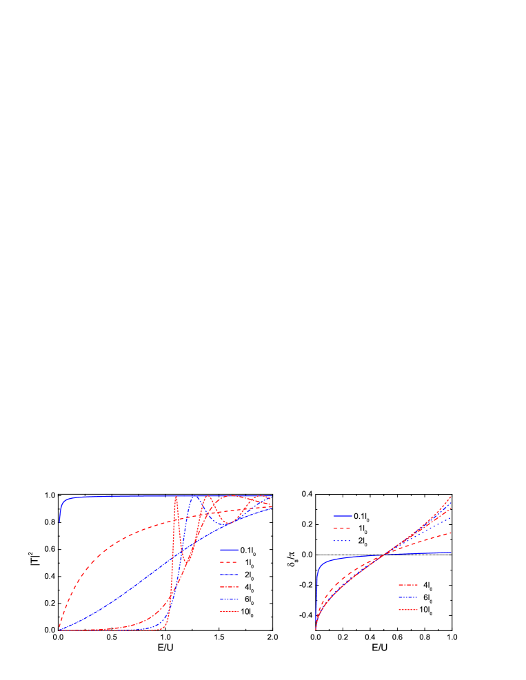
Figure 8: Amplitude and phase of the transmission wave for the rectangular barrier of hight $U$ and length $L$ calculated according to Eqs.  (3.120) and (3.121). Various curves correspond to barriers of different lengths $L$, shown by labels in units of $l_{0}=\hbar/\sqrt{2\,m\,U}$.

Example: scattering on a rectangular barrier

Consider a rectangular potential barrier of length $L$: $U(z)=U=const>0$ for $-L/2<z<L/2$. We assume first that $E<U$. Then we deal with a tunneling problem. The wave function $\psi_{U}$ in internal region, see Eq. (3.106), is decomposed into the following even and odd functions:

$$\chi_{+}(z;E)=\cosh(\varkappa\,z/\hbar)\,,\quad\chi_{-}(z;E)=\sinh(\varkappa\,z/\hbar)\,,\quad\varkappa=\sqrt{2\,m\,(U-E)}>0\,.$$ (3.118)

The logarithmic derivatives follow then as

$$d_{+} = \frac{\varkappa^{2}\,L^{2}}{4\hbar^{2}\,d_{-}}=\frac{\varkappa\,L}{2\hbar}\tanh(\varkappa\,L/2\hbar)\,.$$ (3.119)

The phases of transmitted and reflected amplitudes in (3.111) can now be written through the scattering phase:

$$\delta_{\rm s}(E)=-\arctan\left(\frac{\varkappa^{2}-k^{2}}{2\,k\,\varkappa}\tanh(\varkappa\,L/\hbar)\right)\,.$$ (3.120)

We used here the relation $\tan\big{(}{\pi}/{2}+{\rm arctan}(1/x)\big{)}=-x$ . The squared amplitudes are given by

$$|R|^{2} = \frac{(\varkappa^{2}+k^{2})^{2}}{(\varkappa^{2}-k^{2})^{2}}\sin^{2}\delta_{\rm s}=\frac{(\varkappa^{2}+k^{2})^{2}\,\sinh^{2}(\varkappa\,L/\hbar)}{(\varkappa^{2}+k^{2})^{2}\sinh^{2}(\varkappa\,L/\hbar)+4\,k^{2}\,\varkappa^{2}}\,,$$

$$|T|^{2} = 1-|R|^{2}=\frac{\cos^{2}\delta_{\rm s}}{\cosh^{2}(\varkappa\,L/\hbar)}=\frac{4\,k^{2}\,\varkappa^{2}}{(\varkappa^{2}+k^{2})^{2}\,\sinh^{2}(\varkappa\,L/\hbar)+4\,k^{2}\,\varkappa^{2}}\,.$$ (3.121)

The coefficients $C_{\pm}$ in (3.107) can be expressed now as follows

$$C_{+}=\frac{-ie^{-ik\,L/2\hbar}}{\frac{\varkappa}{k}\,\sinh\big{(}\frac{\varkappa L}{2\,\hbar}\big{)}-i\,\cosh\big{(}\frac{\varkappa L}{2\,\hbar}\big{)}}\,,\quad C_{-}=\frac{ie^{-ik\,L/2\hbar}}{\frac{\varkappa}{k}\,\cosh\big{(}\frac{\varkappa L}{2\,\hbar}\big{)}-i\,\sinh\big{(}\frac{\varkappa L}{2\,\hbar}\big{)}}.$$ (3.122)

The amplitudes $R$ and $T$ can be written as functions of two dimensionless variables characterizing the energy of the incident particle, $E/U$, and the width of the potential, $L/l_{0}$, where $l_{0}=\hbar/\sqrt{2\,m\,U}$. These functions are illustrated in Fig. 8. For a thin barrier, $L\lesssim l_{0}$, the transmission probability is close to unity and the scattering phase is small accept for very small energies. For $E<U$ the transmission probability decreases gradually with an increase of $L$ until $L\simeq 2l_{0}$ and than falls off exponentially for larger $L$. The scattering phase is a monotonously growing function of the energy.

If we replace $\varkappa\to i|\varkappa|$, Eqs. (3.120) and (3.121) also can be used for $E>U$ (scattering above the barrier). For $E>U$, the transmission probability is finite approaching unity for $E\gg U$ unsteadily exhibiting peaks at $E/U=1-\pi^{2}\,n^{2}\,l_{0}^{2}/4\,L^{2}$ with integer $n$. At the peaks $|T|=1$, see Fig. 8.

3.2 Characteristics of time in stationary scattering problem

Within a stationary scattering problem formulated above there is no notion of time per se, since the only $t$ dependent overall factor $e^{-i\,E\,t/\hbar}$ does not enter physical quantities. However, we have at our disposal quantities, which can be used to construct a measure with the dimensionality of time. Such a quantity describing the transmitted waves (at $z>L/2$) arises, for example, if we divide the integral of the squared wave function $\intop_{a}^{b}|\psi(z;E)|^{2}{\rm d}z$ by a current. The flux density outside the barrier does not depend on the coordinate. So we can use expression for the transmitted flux density $j_{\rm T}=|T(E)|^{2}\,k/m$. Then for any interval with $a,b>{\textstyle\frac{1}{2}}L$ the quantity

$$\frac{1}{j_{\rm T}}\intop_{a}^{b}|\psi(z;E)|^{2}{\rm d}z=\frac{b-a}{v}$$ (3.123)

is just a passage time of the segment $[a,b]$ by a particle with the velocity $v=k/m$ . An application of this quantity to the left from the barrier for $a,b<-{\textstyle\frac{1}{2}}L$ could be meaningless, since, e.g., in the case of the full wave reflection from an infinite barrier the total flux vanishes $|j_{\rm I}|-|j_{\rm R}|=j_{\rm T}=0$. On the other hand, the reflected current cannot be used also since it vanishes for the free particle motion. Thus, in order to construct a relevant time-quantity for a particle moving in the segment $[a,b]$ with $a,b<-{\textstyle\frac{1}{2}}L$ we divide the squared wave function by the incident current

$$\frac{1}{j_{\rm I}}\intop_{a}^{b}|\psi(z;E)|^{2}{\rm d}z=\frac{b-a}{v}\,\big{(}1+|R|^{2}\big{)}+\frac{\hbar}{k\,v}\,|R|\,\sin\big{(}2\,k\,z/\hbar-\phi_{\rm R}\big{)}\Big{|}^{b}_{a}\,.$$ (3.124)

The first term represents the passage time of the incident wave in the forward direction through the segment $[a,b]$ (the unity in the brackets) and the passage time of the reflected wave in the backward direction ($|R^{2}|$ in the brackets). For a fully opaque barrier $|R|=1$ we, obviously, get $2(b-a)/v$. The second term appeared due to interference of the incident and reflected waves. It can be neglected only in the short de Broglie wave-length limit $\hbar/k\ll(b-a)$.

Another approach to the definition of time is to introduce an explicit ”clock” – a microscopic device characterized by a simple time variation with a constant well defined period – which is weakly coupled to a quantum system under investigation. From a change of the clock’s ”pointer” one can then read off a duration of the process in the quantum system measured in terms of the clock’s period. Such a procedure was proposed by Salecker and Wigner in [69] for measurements of space-time distances. Peres in [70] extended this concept to several quantum mechanical problems including a time-of-flight measurement of the velocity of a free non-relativistic particle.

Back in 1966, Baz’ [64] proposed the use of the Larmor precession, as a measure of a scattering time in quantum mechanics. He ascribed spin ${\textstyle\frac{1}{2}}$ and a magnetic moment $\mu$ to the scattered particle and assumed presence of a weak magnetic field $B$ within the finite space region of interest, e.g. within a range of potential. The difference in the spin polarization before and after the region proportional to $-{\textstyle\frac{1}{2}}\hbar\omega_{L}\,t_{\rm L}$, where $\omega_{L}=\mu\,B/\hbar$ is the Larmor frequency, gives the time the particle takes to traverse the region. For a one dimensional case this approach was adopted by Rybachenko in Ref. [71]. In the framework of the time-dependent formalism the spin-clock method was analyzed in Ref. [72].

In Ref. [73] Büttiker showed that for a one-dimensional scattering problem the Larmor precession time introduced in [64, 71] is equivalent to the dwell time

$$t_{\rm d}(a,b,E)=\frac{1}{j_{\rm I}}\intop_{a}^{b}|\psi(z;E)|^{2}{\rm d}z\,,$$ (3.125)

which tells how long the incident current $j_{\rm I}$ must be turned on to produce the necessary particle storage within the segment $[a,b]$, see (3.124). This time is a quantum-mechanical counter part of the classical 1D dwell time (2.2). Indeed, as follows from the Schrödinger equation, the probability density given by the square of the wave-function satisfies the continuity equation, as for water in a clepsydra.

The value

$$\delta t_{\rm d}(a,b,E)=t_{\rm d}(a,b,E)-(b-a)/v$$ (3.126)

shows difference of the time, which particle spends in the segment $[a,b]$ of the potential and the time, if the potential in this region were switched off.

For the case $E>\max U$ the classical motion is allowed for any $z$ and the time a particle needs to move from $-L/2$ to $+L/2$ — the classical traversal time — is

$$t_{\rm trav}^{\rm(cl)}(E)=\intop_{-L/2}^{+L/2}\frac{{\rm d}z}{\sqrt{2(E-U(z))/m}}\,,$$ (3.127)

cf. with the definition of the classical sojourn time (2.4). However, when the energy is smaller than a potential maximum, there appears an imaginary contribution to this quantity from the integration between turning points $z_{1}(E)$ and $z_{2}(E)$, which are solutions of the equation $U(z_{1,2})=E$. The imaginary time pattern is used in the so-called imaginary-time formalism, being successfully applied in the problems of quantum tunneling through varying in time barriers, see the review [74]. Nevertheless the imaginary time can be hardly used as the typical time for passing of the barrier.

Ref. [75] considering electron-positron pair production within imaginary time formalism estimated the traversal time of the barrier as its length divided by the velocity of light $c$ (for relativistic particles). The inverse quantity $\omega_{\rm tun}\sim|\nabla U|/mc$ separates then two regimes of particle production in rapidly varying potentials (for $\omega>\omega_{\rm tun}$) and that in static fields (for $\omega\ll\omega_{\rm tun}$). Similarly, Büttiker and Landauer Ref. [76] argued to use the quantity

$$t_{\rm trav}^{\rm(BL)}(E)=\intop_{-L/2}^{+L/2}\frac{{\rm d}z}{\sqrt{2|E-U(z)|/m}}=\int_{-L/2}^{+L/2}\frac{m{\rm d}z}{\varkappa(z,E)}\,$$ (3.128)

for description of the tunneling time trough rapidly varying barriers at a non-relativistic particle motion. Also, they conjectured to use this value to estimate the traversal time of the tunneling through stationary potential barriers. Ref. [77] has shown that this time arises, as a standard dispersion of the tunneling time distribution. A support for the usage of (3.128) to estimate time of particle passage through barriers comes from analysis of the radiation spectral density for charged particles traversing the barrier, which is determined by the ordinary classical formula [78]: $(\partial E_{\omega}/\partial\omega)_{t}\propto e^{2}\omega^{2}k^{2}(t^{\rm BL}_{\rm trav})^{2}/m^{2}$, where $t_{\rm trav}^{\rm BL}$ enters as the time of passing the barrier region.

Also, one can formally construct an analogue of the phase time, as in Eq. (2.57) in Sect. 2, e.g., $\delta t_{\rm ph,R}(E)=\hbar\big{(}\phi_{\rm R}(E)-\pi\big{)}/E$ and $\delta t_{\rm ph,T}(E)=\hbar\big{(}\phi_{\rm T}(E)-\pi\big{)}/E$, as time shifts between incident and reflected and transmitted waves, but these time shifts are not associated with observables.

Relevant quantities are the group times $\hbar{\rm d}\phi_{\rm R}(E)/{\rm d}E$ and $\hbar{\rm d}\phi_{\rm T}(E)/{\rm d}E$, cf. Eq. (2.11), similar to those we introduced in Sect. 2. These quantities will be discussed in a more detail below.

Another part of stationary problems relates to description of bound states arising in case of attractive stationary potentials. Inside the potential well, i.e. for $z\in[z_{1},z_{2}]$, where $z_{1}$ and $z_{2}$ are turning points, the semiclassical wave-function can be written in two ways [79]:

$$\psi^{\rm(scl)}(z;E) = \frac{C_{1}}{\sqrt{|\varkappa(z,E)|}}\cos\Big{(}\intop^{z}_{z_{1}}|\varkappa(z^{\prime},E)|{\rm d}z^{\prime}/\hbar-\phi_{<}\Big{)}\,,$$ (3.129)

or

$$\psi^{\rm(scl)}(z;E) = \frac{C_{2}}{\sqrt{|\varkappa(z,E)|}}\cos\Big{(}\intop_{z}^{z_{2}}|\varkappa(z^{\prime},E)|{\rm d}z^{\prime}/\hbar-\phi_{>}\Big{)}\,,$$ (3.130)

where $\phi_{<}=\phi_{>}=\pi/4$, provided potential is a smooth function of $z$ near turning points. Note that in purely quantum case the phase shifts of in-going and out-going waves for the bound states may depend on $E$. Condition of coincidence of these solutions yields $C_{1}=C_{2}(-1)^{n}$ and we get the Bohr-Sommerfeld quantization rule

$$\int_{z_{1}}^{z_{2}}|\varkappa(z,E)|dz=\hbar(\pi n+\phi_{<}+\phi_{>})\,,\quad n=0,\pm 1,...$$ (3.131)

From this rule for the passage time of the potential well one gets

$$t_{\rm trav}^{\rm(scl)}(z_{1},z_{2},E)={\textstyle\frac{1}{2}}P=\hbar\pi\frac{{\rm d}n}{{\rm d}E}+t_{\rm gr}^{<}+t_{\rm gr}^{>},$$ (3.132)

where $P$ is the period of motion, and $\frac{{\rm d}n}{{\rm d}E}$ is the number of states per unit energy, $t_{\rm gr}^{<}=\hbar{\rm d}\phi_{<}/{\rm d}E$ and $t_{\rm gr}^{>}=\hbar{\rm d}\phi_{<}/{\rm d}E$, and for the semiclassical motion $t_{\rm gr}^{<}+t_{\rm gr}^{>}=0$. Replacing (3.130) with appropriate normalization in (3.125) we get $t_{\rm trav}^{\rm(scl)}(z_{1},z_{2},E)\simeq t_{\rm d}(z_{1},z_{2},E)$.

Example: dwell time for a rectangular barrier

We apply the dwell time definition (3.125) to the wave function  (3.106), (3.118) and calculate the dwell time of the particle under the barrier. The incident current is $j_{\rm I}=k/m$ and

$$t_{\rm d}(-L/2,L/2,E) = \frac{m}{k}\intop_{-L/2}^{+L/2}\Big{\{}|C_{+}|^{2}\,\cosh^{2}(\varkappa\,z/\hbar)+|C_{-}|^{2}\,\sinh^{2}(\varkappa\,z/\hbar)\Big{\}}{\rm d}z$$ (3.133)

$$= \frac{m\,L}{2\,k}\Big{(}|C_{+}|^{2}-|C_{-}|^{2}\Big{)}+\frac{m}{2\,k}\frac{\hbar}{\varkappa}\sinh(\varkappa L/\hbar)\Big{(}|C_{+}|^{2}+|C_{-}|^{2}\Big{)}\,.$$

We see that the dwell time contains two time scales: the one is the free traversal time $m\,L/k$ and the other is a purely quantum scale $m\hbar/k|\varkappa|$. Namely, the former quantity determines the traveling time for classically allowed motion with $E\gg U$. The internal wave function given by Eqs. (3.106) and (3.118), $\psi_{U}$, is expressed in terms of evanescent and growing functions $\psi_{U}^{\rm(evan)}={\textstyle\frac{1}{2}}(C_{+}-C_{-})e^{-\varkappa z/\hbar}$ and $\psi_{U}^{\rm(grow)}={\textstyle\frac{1}{2}}(C_{+}+C_{-})e^{+\varkappa z/\hbar}$. Using Eqs. (3.120) and  (3.122), after some algebra we obtain from Eq. (3.133):

$$t_{\rm d}^{\rm(evan)} = \frac{m}{k}\intop_{-L/2}^{+L/2}{\textstyle\frac{1}{4}}|C_{+}-C_{-}|^{2}e^{-2\varkappa z/\hbar}{\rm d}z=\frac{m\,\hbar}{k\varkappa}\cos^{2}\delta_{\rm s}\frac{k^{2}+\varkappa^{2}}{2\,\varkappa^{2}}\tanh(\varkappa L/\hbar)\frac{e^{\varkappa L/\hbar}}{2\cosh(\varkappa L/\hbar)}\,,$$

$$t_{\rm d}^{\rm(grow)} = \frac{m}{k}\intop_{-L/2}^{+L/2}{\textstyle\frac{1}{4}}|C_{+}+C_{-}|^{2}e^{2\varkappa z/\hbar}{\rm d}z=\frac{m\,\hbar}{k\varkappa}\cos^{2}\delta_{\rm s}\frac{k^{2}+\varkappa^{2}}{2\,\varkappa^{2}}\tanh(\varkappa L/\hbar)\frac{e^{-\varkappa L/\hbar}}{2\cosh(\varkappa L/\hbar)}\,,$$

$$t_{\rm d}^{\rm(evan)} + t_{\rm d}^{\rm(grow)}=\frac{m\,\hbar}{k\varkappa}\cos^{2}\delta_{\rm s}\frac{k^{2}+\varkappa^{2}}{2\,\varkappa^{2}}\tanh(\varkappa L/\hbar)\,,$$ (3.134)

and the correlation term

$$t_{\rm d}^{\rm(cor)}={\textstyle\frac{1}{2}}\Re\{(C_{+}-C_{-})(C_{+}+C_{-})^{*}\}\,L=\frac{m\,L\,}{k}\cos^{2}\delta_{\rm s}\frac{(\varkappa^{2}-k^{2})}{2\varkappa^{2}\cosh^{2}(\varkappa L/\hbar)}\,.$$ (3.135)

Interestingly, the traversal time scale $\propto L$ appears in an interference term $t_{\rm d}^{\rm(cor)}\propto U$ between evanescent and growing waves, whereas the quantum term appears in a sum of the dwell times constructed from the pure evanescent and growing waves, $t_{\rm d}^{\rm(evan)}$ and $t_{\rm d}^{\rm(grow)}$.

For tunneling, $E<U$, through a thick barrier, $\varkappa L/\hbar\gg 1$, we have

$$t_{\rm d}\simeq t_{\rm d}^{\rm(evan)},$$

since $t_{\rm d}^{\rm(cor)}/t_{\rm d}^{\rm(evan)}\sim t_{\rm d}^{\rm(grow)}/t_{\rm d}^{\rm(evan)}\sim e^{-2\varkappa L/\hbar}\ll 1$. The integral in $t_{\rm d}^{\rm(evan)}$ is determined by the region near $z=-L/2$ (provided particles flow on the barrier from the left). Thus in this case the dwell time of particles under the barrier is determined by the inflow near the left edge of the barrier and does not describe particle transmission. This observation a bit corrects statement [8] p. 7, that the dwell time of particles under the barrier ”…does not distinguish transmitted particles from reflected particles” and ”tells us the dwell or sojourn time in the barrier regardless of whether the particle is transmitted or reflected at the end of its stay”.

Combining Eqs. (3.134) and (3.135) we obtain

$$t_{\rm d}(-L/2,L/2,E)=\frac{m\,L\,\cos^{2}\delta_{\rm s}}{2\,k}\left[\frac{k^{2}+\varkappa^{2}}{\varkappa^{2}}\frac{\tanh(\varkappa L/\hbar)}{\varkappa L/\hbar}-\frac{k^{2}-\varkappa^{2}}{\varkappa^{2}}\frac{1}{\cosh^{2}(\varkappa L/\hbar)}\right]\,.$$ (3.136)

Behavior of this value is illustrated in Fig. 9, left. We see that for $E>U$ expression (3.136) exhibits peaks, when the system gets stuck above the barrier in resonance states, for which the barrier becomes effectively absolutely transparent (maxima of $|T|^{2}$ in Fig. 8). The resonance energy is determined by the condition $|\varkappa|L/\hbar=\pi\,n$ for an integer $n>0$. The peak heights increase with the barrier thickness as $(m\,L/k)[1+2L^{2}/(l_{0}^{2}\,n^{2}\,\pi^{2})]$ . The time (3.127) of the traversal of the distance $L$ at resonance energies can be related to the density of the resonance states:

$$t^{\rm(scl)}_{\rm trav}=\frac{Lm}{|\varkappa|}=\pi\hbar\frac{{\rm d}n}{{\rm d}E}\,.$$ (3.137)

For $E\gg U$ we get

$$t_{\rm d}(-L/2,L/2,E)=\frac{mL}{k}\Big{[}1+\frac{U}{2\,E}-\sin(2\varkappa L/\hbar)\frac{l_{0}^{2}}{4L^{2}}\Big{(}\frac{U}{E}\Big{)}^{3/2}+O\Big{(}\frac{U^{2}}{E^{2}}\Big{)}\Big{]}\,.$$ (3.138)

As we see from Fig. 9, for $E>U$ the dwell time oscillates around the classical traversal time and approaches it for $E\gg U$ as

$$\big{|}t_{\rm trav}^{\rm(cl)}(-L/2,L/2,E)-t_{\rm d}(-L/2,L/2,E)\big{|}<\frac{mL}{k}\Big{[}\frac{l_{0}^{2}}{4L^{2}}\Big{(}\frac{U}{E}\Big{)}^{3/2}+O\Big{(}\frac{U^{2}}{E^{2}}\Big{)}\Big{]}\,.$$ (3.139)

For a broad barrier in the limit $|\varkappa|L/\hbar\gg 1$ and for $E\geq U$ we have for the dwell time

$$t_{\rm d}(-L/2,L/2,E_{p})\simeq t_{\rm d}^{\rm(cor)}\simeq\frac{m\,L}{k}\frac{2\,k^{2}\,(k^{2}+|\varkappa|^{2})}{\left[(|\varkappa|^{2}-k^{2})^{2}\sin^{2}(|\varkappa|L/\hbar)+4|\varkappa|^{2}k^{2}\right]}\,.$$ (3.140)

As follows from this expression the dwell time exceeds the classical free traversal time $t_{\rm trav}^{\rm free}=mL/k$.

For $E=U$ and arbitrary $L$ the dwell time is

$$t_{\rm d}(-L/2,L/2,E=U)=\frac{4}{3}\frac{m\,L}{k}\frac{1+3l_{0}^{2}/L^{2}}{1+4l_{0}^{2}/L^{2}}\,.$$ (3.141)

In the tunneling regime $E<U$ the dwell time starts from zero at $E=0$, increases with increase of $E$ and reaches the free traversal time $mL/k$ at

$$E_{1}=U\frac{1+3\,b\,l_{0}^{2}/L^{2}}{1+4\,b\,l_{0}^{2}/L^{2}}\,,\quad b\approx 2.5484\,.$$ (3.142)

It is interesting to note that the dwell time is always smaller than the classical traversal time for energies of the scattered particle $E<U$ for a thick barrier and for $E<{\textstyle\frac{3}{4}}U$  for a thin barrier.

Since in the tunneling regime the dwell time decreases with increase of the barrier depth, and $t_{\rm d}(E\to 0)\to 0$, the dwell time cannot be appropriate measure of the time passage through the barrier.

 

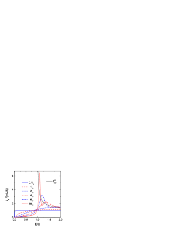
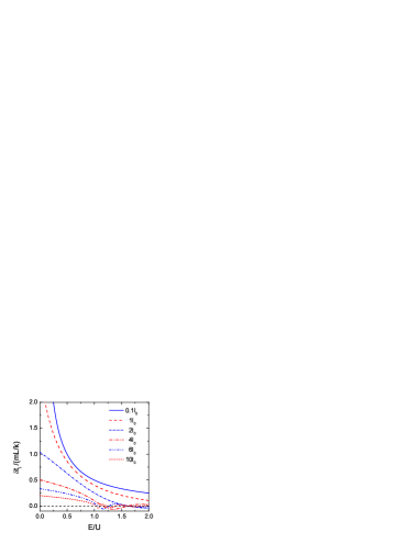
Figure 9: The dwell time (3.136) (left panel) and the interference time (3.172) (right panel) for the rectangular barrier depicted as a function of the energy for various barrier lengths measured in units $l_{0}=\hbar/\sqrt{2\,m\,U}$. The thin solid curve on the left panel shows the classical traversal time (3.127) for the rectangular barrier.

3.3 Non-stationary problem: scattering of a wave packet

The evolution of a quantum-mechanical system from the time moment $t_{0}$ until the time moment $t$ is determined by the Hamilton operator: $\Psi(z,t)=\exp(-i\hat{H}\,(t-t_{0}))\Psi(z,t_{0})$. A non-stationary quantum state, i.e. a state for which physical observables change with time, thus, cannot be an eigenstate of the Hamiltonian. Otherwise the time variations reduce to a phase factor $\exp(-i\,E\,(t-t_{0}))$, which does not enter observables. Hence, in order to describe the passage time of some spatial interval by a quantum particle we need to deal with a wave packet describing by a superposition of stationary states with various energies $E$, $\psi(z;E)$,

$$\Psi(z,t)=\intop_{0}^{\infty}\frac{{\rm d}E}{2\pi\hbar}\Phi(E)\psi(z;E)\,e^{-i\,E\,t/\hbar}\,,$$ (3.143)

with some $\Phi(E)$ as the energy envelop function. Such a packet would necessarily have some spatial extension, which is the larger the smaller is the energy spread of the states collected in the packet. As we discuss in this section, mentioned delocalization makes determination of the passage time of a spatial interval by a quantum particle to be a delicate problem.

As the stationary wave-function $\psi(z;E)$ we can take wave-function (3.100), $\psi(z;E)=C\,\psi_{1}(z,E)$. Normalization constant $C$ can be determined from the relation

$$\intop_{-\infty}^{\infty}{\rm d}z\psi^{*}(z;E)\psi(z;E^{\prime})=2\pi\hbar\sqrt{\frac{2E}{m}}\delta(E-E^{\prime})=2\,\pi\hbar\,\delta(k-k^{\prime})\,,$$ (3.144)

where $k=\sqrt{2mE}$ and $k^{\prime}=\sqrt{2mE^{\prime}}$. The wave function of the wave packet (3.143) can be normalized as

$$\intop_{-\infty}^{\infty}{\rm d}z\,\big{|}\Psi(z,t)\big{|}^{2}=\intop_{0}^{\infty}\frac{{\rm d}E}{2\pi\hbar}\,\sqrt{\frac{2E}{m}}\big{|}\Phi(E)\big{|}^{2}=1\,.$$ (3.145)

Then the quantity

$${\rm d}W_{E}=\sqrt{\frac{2E}{m}}\big{|}\Phi(E)\big{|}^{2}\frac{{\rm d}E}{2\,\pi\,\hbar}$$ (3.146)

is interpreted as the probability for the particle described by the wave packet to have the energy within the segment $[E,E+dE]$. The average energy of the state, $\overline{E}$, is given by

$$\overline{E}=\intop_{-\infty}^{\infty}{\rm d}x\Psi^{*}(x,t)\hat{H}\Psi(x,t)=\intop_{0}^{\infty}\frac{{\rm d}E}{2\pi\hbar}E\,\sqrt{\frac{2E}{m}}\big{|}\Phi(E)\big{|}^{2}\,.$$ (3.147)

Similarly, the energy dispersion of the wave packet is given by

$$\gamma^{2}=\intop_{-\infty}^{\infty}{\rm d}x\,\Psi^{*}(x,t)\,\big{(}\hat{H}^{2}-\overline{E}^{2}\big{)}\,\Psi(x,t)=\intop_{0}^{\infty}\frac{{\rm d}E}{2\pi\hbar}\big{(}E^{2}-\overline{E}^{2}\big{)}\,\sqrt{\frac{2E}{m}}\big{|}\Phi(E)\big{|}^{2}\,.$$ (3.148)

Formally, we can change an integration variable from $E$ to $k=\sqrt{2\,m\,E}$ and rewrite the distribution (3.146) as

$${\rm d}W_{E}=\big{|}\varphi(k)\big{|}^{2}\frac{{\rm d}k}{2\,\pi\,\hbar}\,,\quad\varphi(k)=\frac{k}{m}\Phi(k^{2}/2m),$$ (3.149)

and the wave packet (3.143), as

$$\Psi(z,t)=\intop_{0}^{\infty}\frac{{\rm d}k}{2\pi\hbar}\,\varphi(k)\,\psi(z;k^{2}/2m)\,e^{-i\,k^{2}t/2m\hbar}\,.$$ (3.150)

We emphasize that the quantity $\big{|}\varphi(k)\big{|}^{2}$ cannot be identified with a momentum distribution of the state, since in general the wave function $\psi(z;E=k^{2}/2m)$ is not an eigen function of the momentum operator. However, in the remote past, i.e., for large and negative $t$, when the peak of the packet is at large and negative $z\ll-L$, we deal with a free wave packet. Then only one term of the wave function (3.100) contributes to the integral (3.150). Indeed, only in the term proportional to $e^{i\,k\,z}$ for $z\ll-L$ the exponents under the integral in Eq. (3.150) can cancel each other for $z\sim t\,k/m$. Thus, in the past the maximum of the packet located far to the left from the barrier, — an incident wave packet

$$\Psi(z,t)\approx\Psi_{\rm I}(z,t)=\intop_{0}^{\infty}\frac{{\rm d}k}{2\pi\hbar}\,\varphi(k)\,e^{ik\,z/\hbar}e^{-i\,k^{2}t/2m\hbar}\,,$$ (3.151)

moves to the right. In this limit the quantity $\big{|}\varphi(k)\big{|}^{2}$ defines the asymptotic momentum distribution in the packet. Note that there is always a small but finite probability for the particle to be in any point of the $z$ axes.

The momentum average and variance are then given by

$$p=\langle k\rangle_{k}\,,\quad\gamma_{p}^{2}=\langle(k^{2}-p^{2})\rangle_{k}\,.$$ (3.152)

Here we use the notation

$$\big{\langle}\dots\big{\rangle}_{k}=\intop_{0}^{\infty}\frac{{\rm d}k}{2\,\pi\,\hbar}\,\big{(}\dots\big{)}\,\big{|}\varphi(k)\big{|}^{2}$$ (3.153)

for the average over the momentum distribution. The average energy and momentum are related as $\overline{E}=(p^{2}+\gamma_{p}^{2})/2m$ . For evaluation of the $k$-averages (3.153) of a function $f$ dependent on $k$ we can use the relation

$$\langle f(k)\rangle_{k}\approx f(p)+\frac{1}{2}\gamma_{p}^{2}\frac{{\rm d}^{2}f(p)}{{\rm d}p^{2}}=f(E_{p})+\frac{\gamma_{p}^{2}}{2\,m}\frac{{\rm d}f(E_{p})}{{\rm d}E_{p}}+\frac{\gamma_{p}^{2}\,p^{2}}{2\,m^{2}}\frac{{\rm d}^{2}f(E_{p})}{{\rm d}E_{p}^{2}}\,,$$ (3.154)

provided $\gamma_{p}$ is small. We used Eq. (3.152) and in the second equality we changed variables from $p$ to $E_{p}=p^{2}/2m$.

The momentum profile function $\varphi(k)$ is complex, $\varphi(k)=|\varphi(k)|\,e^{i\xi(k)}$. The derivative of its phase with respect to momentum, $\xi^{\prime}(k)$, determines the average coordinate of the incident packet [80]

$$\bar{z}_{\rm I}(t) = \intop^{-L/2}_{-\infty}{\rm d}z\,z|\Psi_{\rm I}(z,t)|^{2}/\intop_{-\infty}^{-L/2}{\rm d}z\,|\Psi_{\rm I}(z,t)|^{2}\approx\bar{z}_{\rm I}^{\rm(as)}(t)=\intop_{-\infty}^{+\infty}{\rm d}z\,z|\Psi_{\rm I}(z,t)|^{2}$$ (3.155)

$$= \big{\langle}-\hbar\xi^{\prime}(k)+\frac{k}{m}\,t\big{\rangle}_{k}=\langle-\hbar\xi^{\prime}(k)\rangle_{k}+v_{\rm I}\,t\,,\quad v_{\rm I}=\frac{p}{m}\,.$$

Note that the second approximate equality in the first line is valid, if at time $t$ the packet is located almost entirely to the left from the barrier. It is valid for $\gamma_{p}(-z_{0}+L)\gg\hbar$ for large negative $t$. The derivation of this relation is given in Appendix C. Let us fix the phase $\xi(k)$ so that in the remote past at $t_{0}$ the packet center was at $z_{\rm 0}=v_{\rm I}\,t_{0}$, then $-\hbar\xi^{\prime}(k)=z_{0}-k\,t_{0}/m$ and therefore $\langle-\hbar\xi^{\prime}(k)\rangle_{k}=0.$

The evolution of the packet width in the coordinate space is determined by the function $\varphi(k)$ as

$$\overline{z_{\rm I}^{2}}(t)-\bar{z}_{\rm I}^{2}(t) \approx \frac{\hbar}{4\pi}|\varphi(0)|^{\prime}|\varphi(0)|+\hbar^{2}\Big{\langle}\Big{(}\frac{|\varphi(k)|^{\prime}}{|\varphi(k)|}\Big{)}^{2}\Big{\rangle}_{k}+\Big{\langle}\Big{(}\hbar\xi^{\prime}(k)-\frac{k}{m}\,t\Big{)}^{2}\Big{\rangle}_{k}-\Big{\langle}\Big{(}\hbar\xi^{\prime}(k)-\frac{k}{m}\,t\Big{)}\Big{\rangle}^{2}_{k}\,.$$ (3.156)

For description of a remote solitary incident packet moving to the right with an initial average energy $\simeq\overline{E}$ the envelop function $\Phi(E)$ must be sharply peaked at $E=\overline{E}$, or equivalently for the description of the packet moving with the average momentum $p$ the function $\varphi(k)$ must be sharply peaked at $k=p$. If the widths of the peaks of the functions $\Phi(E)$ and $\varphi(k)$ are sufficiently small, i.e. $\gamma_{p}\ll p$ and $\gamma\ll\overline{E}$, the lower limit in all momentum and energy integrations can be extended to $-\infty$. Often, the normalized momentum profile function is chosen in the Gaussian form

$$\varphi(k)=\Big{(}\frac{2\,\pi\,\hbar^{2}}{\gamma_{p}^{2}}\Big{)}^{1/4}\,\exp\Big{(}-\frac{(k-p)^{2}}{4\,\gamma_{p}^{2}}+i\,\xi(k)\Big{)}\,.$$ (3.157)

Then, using that $-\hbar\xi^{\prime}(k)=z_{0}-k\,t_{0}/m$ we find from Eq. (3.156)

$$\overline{z_{\rm I}^{2}}(t)-\bar{z}_{\rm I}^{2}(t)=\frac{\hbar^{2}}{4\,\gamma_{p}^{2}}+\frac{\gamma_{p}^{2}}{m^{2}}\,(t-t_{0})^{2}\,,$$ (3.158)

where we used that for a narrow packet $|\varphi(0)|\to 0$ . We recover the well-known result that the width of a free packet increases with time. For the typical time of the smearing of the packet we immediately get $t-t_{0}\sim t_{\rm sm}$, where

$$t_{\rm sm}=\hbar\,m/\gamma_{p}^{2}\,.$$ (3.159)

3.4 Characteristics of time for scattering of a wave packet with negligibly small momentum uncertainty

Consider a wave packet (3.150) prepared far away from the potential region, so that the packet could be made sufficiently broad to assure a small momentum uncertainty and at the same time it would take a long time for the packet to reach the potential barrier. After the wave packet has reached the barrier it is split into the reflected wave packet and two forward going (evanescent and growing) waves propagating under the barrier, which outside of the barrier transform to a transmitted wave packet.

The transmitted packet is determined by [81]

$$\Psi_{\rm T}(z,t)=\intop_{0}^{\infty}\frac{{\rm d}k}{2\pi\hbar}\varphi(k)|T(E)|e^{i\phi_{\rm T}(E)}e^{ikz/\hbar-iEt/\hbar}\,.$$ (3.160)

The reflected packet moving backwards is

$$\Psi_{\rm R}(z,t)=\intop_{0}^{\infty}\frac{{\rm d}k}{2\pi\hbar}\varphi(k)|R(E)|e^{i\phi_{\rm R}(E)}e^{-ikz/\hbar-iEt/\hbar}\,,$$ (3.161)

where, as before, $E=k^{2}/2m$.

Also, one can introduce two measures of time that could characterize the wave propagation within the potential region. Consider the difference of the time, when the maximum of the incident packet (3.151) is at the coordinate $z=-L/2$, and the time, when the maximum of the transmitted packet (3.160) is at $z=+L/2$, and the difference of the time, when the maximum of the incident packet and the maximum of the reflected packet (3.161) are at the same spatial point $z=-L/2$. We call these time intervals the transmission and reflection group times, $t_{\rm T}$ and $t_{\rm R}$. The construction of the delay times goes back to pioneering works by Eisenbud [82], Wigner [1] and Bohm [81]. According to the method of stationary phase, the position of the maximum of an oscillatory integral, as those in Eqs. (3.151), (3.160), and (3.161), is determined by the stationarity of the complex phase of the integrand. For sufficiently narrow initial momentum distribution, $\gamma_{p}\ll p$, we can write

$$t_{\rm T}(E_{p})=\Big{(}\hbar\xi^{\prime}(p)+\frac{L}{2\,v_{\rm I}}+\frac{\hbar}{v_{\rm I}}\frac{{\rm d}}{{\rm d}p}\phi_{\rm T}(E_{p})\Big{)}-\Big{(}\hbar\xi^{\prime}(p)-\frac{L}{2\,v_{\rm I}}\Big{)}=\frac{L}{v_{\rm I}}+\hbar\frac{{\rm d}\phi_{\rm T}(E_{p})}{{\rm d}E_{p}}\,,$$ (3.162)

and

$$t_{\rm R}(E_{p})=\Big{(}\hbar\xi^{\prime}(p)+\frac{L}{2\,v_{\rm I}}+\frac{\hbar}{v_{\rm I}}\frac{{\rm d}}{{\rm d}p}\phi_{\rm R}(E_{p})\Big{)}-\Big{(}\hbar\xi^{\prime}(p)-\frac{L}{2\,v_{\rm I}}\Big{)}=\frac{L}{v_{\rm I}}+\hbar\frac{{\rm d}\phi_{\rm R}(E_{p})}{{\rm d}E_{p}}\,,$$ (3.163)

here and below $E_{p}=p^{2}/2m$. For $E_{p}\gg U$, $\frac{{\rm d}\phi_{\rm T,R}(E_{p})}{{\rm d}E_{p}}\to 0$ and $t_{\rm T}(E_{p})\simeq t_{\rm R}(E_{p})\simeq\frac{L}{v_{\rm I}}$ reduce to the passage time of the distance $L$. However, interpretation of these times for $E<U$ needs a special care. Recall that in case of the tunneling the transmission and reflection group times $t_{\rm T}(E_{p})$ and $t_{\rm R}(E_{p})$ are asymptotic quantities since they count time steps for events happened at $z=-L/2$ and $z=L/2$ rather than at the turning points. Moreover, as we shall see, for the tunneling through thick barriers the dependence of these times on $L$ ceases.

One can introduce conditional transmission and reflection group times by multiplying the times $t_{\rm T}$ and $t_{\rm R}$ with the transmission and reflection probabilities, respectively. Summing them up we define a bidirectional scattering time, as the sum of the weighted average of transmitted and reflected group delays [8]

$${t}_{\rm bs}(E_{p})=|T(E_{p})|^{2}\,t_{\rm T}(E_{p})+|R(E_{p})|^{2}\,t_{\rm R}(E_{p})\,.$$ (3.164)

This time can be also expressed through the induced, transmitted and reflected currents defined for the stationary problem, see Eq. (3.105),

$${t}_{\rm bs}=\frac{j_{\rm T}}{j_{\rm I}}\,t_{\rm T}+\frac{|j_{\rm R}|}{j_{\rm I}}\,t_{\rm R}.$$ (3.165)

For symmetrical barrier with the help of Eqs. (3.111) and (3.112) we get

$$t_{\rm bs}(E_{p})=t_{\rm T}(E_{p})=t_{\rm R}(E_{p})=\hbar\frac{{\rm d}\delta_{\rm s}(E_{p})}{{\rm d}E_{p}}\,.$$ (3.166)

We should emphasize a direct correspondence of the transmission and reflection group times defined here to the classical group times defined in Eqs. (2.21) and (2.66). For $E_{p}\gg U$, $\hbar\frac{{\rm d}\delta_{\rm s}(E_{p})}{{\rm d}E_{p}}\to L/v_{\rm I}$.

There is a relation [83, 84] between the bidirectional scattering time $t_{\rm bs}$, Eq. (3.164), and the dwell time $t_{\rm d}$, Eq. (3.125), which follows from the general relation for the stationary wave function (3.115) and definitions (3.162), (3.163):

$$t_{\rm d}(-L/2,L/2,E_{p})=t_{\rm bs}(E_{p})-\delta t_{\rm i}(E_{p})\,.$$ (3.167)

The last term here is the interference time delay. It arises due to the interference of the incident part of the wave function (the incident packet) with its reflected part. This term is of the same origin as the last term on the left-hand side of Eq. (3.124),

$$\delta t_{\rm i}(E_{p})=-\frac{\hbar}{pv_{\rm I}}\,\Im\big{(}R(E_{p})e^{+i\,p\,L/\hbar}\big{)}=-\frac{\hbar\,}{pv_{\rm I}}|R(E_{p})|\sin\big{(}\phi_{\rm R}(E_{p})+p\,L/\hbar\big{)}\,.$$ (3.168)

The interference time can be as positive as negative, so it represents delay or advance of the incident packet. This term $\delta t_{\rm i}$ is especially important for low energies (small momenta), when the packet approaches the barrier very slowly. Taking into account that $|T|^{2}+|R|^{2}=1$ we can rewrite Eq. (3.167) in the form

$$t_{\rm d}=|T|^{2}\,(t_{\rm T}-\delta t_{\rm i})+|R|^{2}\,(t_{\rm R}-\delta t_{\rm i}).$$ (3.169)

The times $(t_{\rm T}-\delta t_{\rm i})$ and $(t_{\rm R}-\delta t_{\rm i})$ coincide with the Larmor times introduced by Baz’ and Rybachenko [64, 71] in general case of asymmetric potentials. Naively [61], one interprets result (3.169), as the time spend by the particle under the barrier ($t_{\rm d}$) is the sum of the tunneling traversal time in transmission $t_{\rm T}-\delta t_{\rm i}$ times probability of transmission and the tunneling traversal time in the reflection $t_{\rm R}-\delta t_{\rm i}$ times probability of reflection. Such an interpretation is actually false, since in quantum mechanics one should sum amplitudes rather than probabilities [8]. Moreover, as we mentioned, for thick barriers $t_{\rm d}$ is almost entirely determined by the behavior of the wave function on the left edge of the barrier and thereby does not relate to the transmission process. Else, $t_{\rm T}$ and $t_{\rm R}$ are determined when the peaks of packets are at $z=\pm L/2$ rather than at the turning points and thereby they cannot control only the tunneling.

Some authors, see [85, 86, 87], introduce tunneling transit times by dividing the probability stored within the potential region by the local transmitted flux and the reflected flux

$$\widetilde{t}_{\rm T}=\frac{1}{j_{\rm T}}\int_{-L/2}^{L/2}{\rm d}z|\psi(z,E_{p})|^{2}=\frac{t_{\rm d}}{|T|^{2}},\quad\widetilde{t}_{\rm R}=\frac{1}{|j_{\rm R}|}\int_{-L/2}^{L/2}{\rm d}z|\psi(z,E_{p})|^{2}=\frac{t_{\rm d}}{|R|^{2}}\,,$$ (3.170)

from where we get $t_{\rm d}^{-1}=\widetilde{t}_{\rm T}^{-1}+\widetilde{t}_{\rm R}^{-1}$. It follows from analogy with fluid mechanics: the local velocity $v(z)$ is related to the local density $\rho=|\psi(z)|^{2}$ through $j=\rho v$, see (2.2). Since $|T|^{2}$ is exponentially small for a broad barrier, $\widetilde{t}_{\rm T}$ is exponentially large in this case. It is perfectly luminal and does not saturate with barrier length [84]. Ref. [8] argues that the quantities (3.170) characterize net-delays of transmitted and reflected fluxes rather than tunneling times. Indeed the time $\widetilde{t}_{\rm T}$ is a property of entire wave function made up of forward and backward going components and thereby cannot be considered as traversal time of transmitted particles only [8]. Performing minimization of $\widetilde{t}_{\rm T}$, Ref.  [88] finds a variationally determined tunneling time $\widetilde{t}_{\rm T}^{\rm min}\propto 1/|T|$. Both $\widetilde{t}_{\rm T}$ and $\widetilde{t}_{\rm T}^{\rm min}\to\infty$ for $|T|\to 0$. Note that the typical time after passing of which we are able to observe the particle with probability of the order of one to the right from the barrier, if it initially were to the left from the barrier is indeed proportional to $1/|T|^{2}$. But the time $\propto 1/|T|^{2}$ does not correspond to our expectations for the quantity characterizing traversal time of the given particle from $a$ to $b$. It is associated with the life-time of metastable states, being in this case the tunneling particles treated as quasiparticles decaying from a state on one side of the barrier into another state on other side of the barrier [63]. This time represents a mean time, in which a certain likelihood of a tunneling event may take place. After passage of this time it becomes probable that approximately a half of the original particle density has managed to tunnel away. This does not reflect actual time of the tunneling.

Example 1: group times for a rectangular barrier
The scattering phase for a rectangular barrier is given in Eq. (3.120). Substituting this expression in Eq. (3.166) we find

$$t_{\rm bs}=t_{\rm T}=t_{\rm R}=\frac{L\cos^{2}\delta_{\rm s}}{2\,v_{\rm I}}\left[\frac{(p^{2}+\varkappa^{2})^{2}}{p^{2}\varkappa^{2}}\frac{\tanh(\varkappa L/\hbar)}{\varkappa L/\hbar}-\frac{p^{2}-\varkappa^{2}}{\varkappa^{2}}\frac{1}{\cosh^{2}(\varkappa L/\hbar)}\right]\,.$$ (3.171)

The interference time (3.168) can be written as

$$\delta t_{\rm i}=\frac{L}{v_{\rm I}}\cos^{2}\delta_{\rm s}\frac{p^{2}+\varkappa^{2}}{2\,p^{2}}\frac{\tanh(\varkappa L/\hbar)}{\varkappa L/\hbar}\,.$$ (3.172)

For $E_{p}\ll U$, performing expansion in $E_{p}/U$ we have

$$\delta t_{\rm i}\approx 2\frac{l_{0}}{v_{\rm I}}\coth(L/l_{0})-\frac{l_{0}}{v_{\rm I}}\Big{(}\coth(L/l_{0})+(8\coth(L/l_{0})-L/l_{0})/\sinh^{2}(L/l_{0})\Big{)}\frac{E_{p}}{U}\,.$$ (3.173)

The interference time is shown in Fig. 9, right, as a function of $E_{p}/U$ for various barrier lengths. As we see, the interference time is especially significant for small energies when the incident packet approaches the barrier slowly. For $E_{p}<U$, $\delta t_{\rm i}>0$, for $E_{p}>U$, at some energies $\delta t_{\rm i}$ becomes negative. For $E_{p}\gg U$, $\delta t_{\rm i}\to 0$ and $t_{\rm bs}\simeq t_{\rm d}\simeq L/v_{\rm I}$.

Example 2: group times in the semi-classical approximation
The wave function of the stationary scattering problem, which enters the wave packet (3.143), can be written in the semiclassical approximation as follows [51]

$$\psi^{\rm(scl)}(z;E_{p}) = \left\{\begin{array}[]{lll}\sqrt{\frac{m}{|\varkappa(z,E_{p})|}}\left[e^{\frac{i}{\hbar}\int_{z_{1}}^{z}|\varkappa(z^{\prime},E_{p})|{\rm d}z^{\prime}+i\phi_{0}}+e^{-\frac{i}{\hbar}\intop_{z_{1}}^{z}|\varkappa(z^{\prime},E)|{\rm d}z^{\prime}-i\phi_{0}}\right]&,&z<z_{1},\\ \sqrt{\frac{D\,m}{\varkappa(z,E_{p})}}\,e^{\intop^{z_{2}}_{z}\varkappa(z^{\prime},E_{p}){\rm d}z^{\prime}/\hbar}&,&z_{1}\leq z\leq z_{2},\\ \sqrt{\frac{D\,m}{|\varkappa(z,E_{p})|}}\,e^{\frac{i}{\hbar}\intop_{z_{2}}^{z}|\varkappa(z^{\prime},E_{p})|{\rm d}z^{\prime}+i\phi_{0}}&,&z_{2}\leq z\,,\end{array}\right.$$ (3.178)

$$D=\exp\Big{(}-\frac{2}{\hbar}\int_{z_{1}}^{z_{2}}\varkappa(z^{\prime},E_{p}){\rm d}z^{\prime}\Big{)}\,,$$

where $z_{1}$ and $z_{2}$ are the left and right turning points ($z_{1}<z_{2}$) and the phase $\phi_{0}=\pi/4$ for a smooth scattering potential, cf. Eq. (3.130). Note that in the framework of the semiclassical approximation  [51] it is legitimate to take into account only evanescent wave inside the barrier. Being derived with the same accuracy, the reflection coefficient equals unity. Respectively, the incident current is then totally compensated by the reflected one and the current inside the barrier is absent, whereas it is present outside the barrier for $z>z_{2}$. This current non-conservation is inconvenient, when we study particle propagation inside the barrier. To recover the current conservation one should include the contribution of the growing wave inside the barrier, despite this procedure is beyond the scope of the formal applicability of the semiclassical approximation, see [7]. Similarly, in non-equilibrium quantum field description one introduces so called self-consistent approximations to keep the conservation laws on exact level, see [33, 34, 35, 36, 37] and discussion in Sect. 6.

Repeating the procedure that leads to Eqs. (3.162) and (3.163) from (3.178) we obtain

$$t^{\rm(scl)}_{\rm T} = \Big{(}\hbar\xi^{\prime}(p)+\frac{1}{v_{\rm I}}\frac{{\rm d}}{{\rm d}p}\intop_{z_{2}}^{z}|\varkappa(z^{\prime},E_{p})|{\rm d}z^{\prime}\Big{)}\Bigg{|}_{z=z_{2}}-\Big{(}\hbar\xi^{\prime}(p)+\frac{1}{v_{\rm I}}\frac{{\rm d}}{{\rm d}p}\int_{z_{1}}^{z}|\varkappa(z^{\prime},E_{p})|{\rm d}z^{\prime}\Big{)}\Bigg{|}_{z=z_{1}}=0\,,$$

$$t^{\rm(scl)}_{\rm R} = \Big{(}\hbar\xi^{\prime}(p)+\frac{1}{v_{\rm I}}\frac{{\rm d}}{{\rm d}p}\intop_{z_{1}}^{z}|\varkappa(z^{\prime},E_{p})|{\rm d}z^{\prime}\Big{)}\Bigg{|}_{z=z_{1}}-\Big{(}\hbar\xi^{\prime}(p)-\frac{1}{v_{\rm I}}\frac{{\rm d}}{{\rm d}p}\int_{z_{1}}^{z}|\varkappa(z^{\prime},E_{p})|{\rm d}z^{\prime}\Big{)}\Bigg{|}_{z=z_{1}}=0\,.$$ (3.179)

We see that within semiclassical approximation $t^{\rm(scl)}_{\rm T}=t^{\rm(scl)}_{\rm R}=t^{\rm(scl)}_{\rm bs}=0$, if we compare the moments of time, when the maxima of the packets are at the turning points. This was first announced in [89] but basing on this fact concluded that the tunneling time in semiclassical approximation is zero. In our opinion, being zero, the quantity $t_{\rm T}^{\rm(scl)}$, as well as $t_{\rm T}$, can hardly be considered as appropriate characteristic of the time passage of the barrier. The values $t^{\rm(scl)}_{\rm T}=t^{\rm(scl)}_{\rm R}=0$ just show that the delay of wave packets within the region of finite potential appears due to purely quantum effects, being vanishing in semiclassical approximation. It also demonstrates that in case of the tunneling the group delays are accumulated in the region near the turning points where semiclassical approximation is not applicable.

Finally, we repeat that in general case the reflection group time shows nothing else that a time delay between formation of the peak of the reflected wave at $z=-L/2$ compared to the moment, when the incident wave peak reached $z=-L/2$. The transmission group time demonstrates difference of time moments, when the peak of the transmission wave starts its propagation at $z=L/2$ and the incident wave peak reaches $z=-L/2$. In semiclassical approximation these time delays are absent.

3.5 Sojourn time for scattering of an arbitrary wave-packet

So far we have considered the time-like quantities, which are precise only to the extend that the packet has a small momentum uncertainty, as the group times [Eqs. (3.162), (3.163), and (3.166)] [61], and the dwell time [Eq. (3.125)], originated within stationary problem. Nevertheless it is possible to introduce another time-like quantity, which measures how long the system stays within a certain coordinate region. In classical mechanics the time, which a system committing 1D motion spends within the segment $[a,b]$, is determined by the integral (2.3). In quantum mechanics the $\delta$-function over the classical trajectory is to be replaced with the quantum probability density $|\Psi(z,t)|^{2}$, see [90]. Now, if we consider a wave packet starting from the left at large negative $z$ for large negative $t$ and proceeding to $z=+\infty$, then the time it spends within the segment $[a,b]$ is given by the quantum mechanical sojourn time defined as

$$t_{\rm soj}(a,b)=\intop_{-\infty}^{+\infty}{\rm d}t\intop_{a}^{b}{\rm d}z|\Psi(z,t)|^{2}\,.$$ (3.180)

The packet wave function is normalized as (3.145). Between the dwell time and the sojourn time there is a relation [91], see derivation in Appendix D,

$$t_{\rm soj}(a,b)=\intop_{-\infty}^{+\infty}\frac{{\rm d}k}{2\pi\hbar}|\varphi(k)|^{2}t_{\rm d}(a,b,k^{2}/2m)=\big{\langle}t_{\rm d}(a,b,k^{2}/2m)\big{\rangle}_{k}\,.$$ (3.181)

Using that the wave function obeying the Schrödinger equation satisfies the continuity equation

$$\frac{{\rm d}}{{\rm d}t}|\Psi(z,t)|^{2}=-\frac{{\rm d}}{{\rm d}z}j(z,t)\,,$$ (3.182)

where $j(z,t)=\mathcal{J}[\Psi(z,t)]$ with the current $\mathcal{J}$ defined in (3.105), we can rewrite the sojourn time through the currents on the borders of the interval

$$t_{\rm soj}(a,b)=-\intop_{-\infty}^{+\infty}{\rm d}t\intop_{-\infty}^{t}{\rm d}t^{\prime}\big{[}j(b,t^{\prime})-j(a,t^{\prime})\big{]}\,.$$ (3.183)

From these relations we see that the sojourn time, has the same deficiencies, as the dwell time. Namely, for a broad barrier both quantities demonstrate how long it takes for the particles to enter the barrier from the left end, but they do not describe particle transmission to the right end.

We now apply the relation (3.183) and the sojourn time definition to the wave function (3.100). The total time, which the packet spends in the barrier region, $-L/2\leq z\leq L/2$, is $t_{\rm soj}(-L/2,L/2)=\big{\langle}t_{\rm d}(-L/2,L/2,k^{2}/2m)\big{\rangle}_{k}$. As we show in Appendix D the integration of currents in Eq. (3.183) gives [80]

$$\intop_{-\infty}^{+\infty}{\rm d}t\!\!\intop_{-\infty}^{t}\!\!{\rm d}t^{\prime}\Big{(}j(L/2,t^{\prime})-j(-L/2,t^{\prime})\Big{)}=-\big{\langle}|T(E)|^{2}\,t_{\rm T}(E)\big{\rangle}_{k}-\big{\langle}|R(E)|^{2}\,t_{\rm R}(E)\big{\rangle}_{k}+\big{\langle}\delta t_{\rm i}(E)\big{\rangle}_{k}\,.$$ (3.184)

Thus, in case of an arbitrary momentum distribution we obtain generalization of Eqs. (3.167) and (3.168):

$$t_{\rm soj}(-L/2,L/2)=\big{\langle}t_{\rm d}(-L/2,L/2,E_{k})\big{\rangle}_{k}=\big{\langle}|T(E)|^{2}\,t_{\rm T}(E)\big{\rangle}_{k}+\big{\langle}|R(E)|^{2}\,t_{\rm R}(E)\big{\rangle}_{k}-\big{\langle}\delta t_{\rm i}(E)\big{\rangle}_{k}\,.$$ (3.185)

Thereby, from definition of the sojourn time we extract the same information as from definition of the dwell time but averaged over energies of the packet. We stress that both quantities do not describe time of the particle passage of the barrier.

3.6 The Hartman effect

For energies above the barrier the proper time for the particle to pass the region of the potential is the traversal time $t_{\rm trav}^{\rm(cl)}$. Other times $t_{\rm d}(-L/2,L,E_{p})$, $t_{\rm soj}(-L/2,L,E_{p})$, $t_{\rm bs}(E_{p})$ introduced above also appropriately characterize the particle motion. For energies well above the barrier, $E\gg U$, we find $t_{\rm trav}^{\rm(cl)}\simeq t_{\rm bs}(E_{p})\simeq t_{\rm d}(-L/2,L,E_{p})\simeq L/v_{\rm I}$. However there appear problems with interpretation of all these times, as a characteristic of a particle’s passage under the barrier (for $E<U$).

In numerous works the dwell time was interpreted as a mean time the particle spends under the barrier regardless of whether it is ultimately transmitted or reflected, see discussion in Ref. [8]. The link (3.169) between the dwell time and the group times suggested a naive interpretation of the times $t_{\rm T}-\delta t_{\rm i}$ and $t_{\rm R}-\delta t_{\rm i}$ as mean times the transmitted and reflected particles spend under the barrier. As we mentioned, such an interpretation is based on a classical counting of possible outcomes of a scattering process in 1D, when an incident particle can be either reflected or transmitted, cf. Sec. IIIB in Ref. [61]. Accepting such an interpretation of the group and dwell times one encounters a paradox. In order to understand it more clearly consider tunneling ($E<U$) through a thick rectangular barrier $\varkappa L/\hbar=\sqrt{1-E_{p}/U}L/l_{0}\gg 1$. From Eqs. (3.120), (3.166) and (3.169) we find

$$t_{\rm d}(-L/2,L/2,E_{p})=t_{\rm T}(E_{p})-\delta t_{\rm i}(E_{p})=t_{\rm R}(E_{p})-\delta t_{\rm i}(E_{p})=\frac{p^{2}}{p^{2}+\varkappa^{2}}\hbar\frac{{\rm d}\delta_{\rm s}(E_{p})}{{\rm d}E_{p}},$$

$$t_{\rm bs}(E_{p})=t_{\rm T}(E_{p})=t_{\rm R}(E_{p})\simeq\hbar\frac{{\rm d}\delta_{\rm s}(E_{p})}{{\rm d}E_{p}}=2\frac{\hbar}{v_{\rm I}\varkappa}\,.$$ (3.186)

The characteristic length entering these expressions is the quantum depth of particle penetration inside the barrier region $\sim\hbar/\varkappa$ rather than the length of the barrier $L$. Therefore all these characteristic times are reduced to the quantum time $t_{\rm quant}\sim\hbar/v_{\rm I}\varkappa$ not proportional to the barrier length $L$, as one could expect for a proper passage time of the distance $L$ with a constant velocity. This would mean that, being evaluated with the help of these times, the average velocity of the particle passage of the barrier would exceed the speed of light for sufficiently large $L$. Such a phenomenon first described in Ref. [13] was then called the Hartmann effect. The effect survives independently of the specific form of the potential. The same effect arises, if one uses the relativistic Dirac and Klein-Gordon equations instead of the Schrödinger equation [92]. As Winful writes [8]: ”Because of this apparent superluminality, there are some who dismiss it as a relevant time scale for the tunneling process. This is part of the motivation for the ongoing search of other tunneling times.”

The Hartman effect has not yet been observed for matter waves. However, one has used the identity of the form of the Helmoltz equation for wave propagation in a bulk inhomogeneous medium and the time-dependent Schrödinger equation, and studied the tunneling of electromagnetic waves through a barrier. Reference [93] reported that a superluminal tunneling of light was observed, that caused a vivid discussion in the literature, see for example reviews [10, 11]. The group velocity may become superluminal and even negative without any contradiction with causality [62, 6, 94]. General arguments [95] based on unitarity and causality show that the peak of the transmitted pulse is constructed mainly from leading edge of the incident one. Namely, pulse reshaping leading to apparent causality was found in absorbing or amplifying media whose relaxation times are long compared with pulse duration. For thorough analysis of the Hartman effect and re-interpretations of the experiments free of problems with causality we refer the reader to the review of Winful  [8]. The saturation of the group delay with the barrier length is explained by the saturation of the stored energy. The Winful’s argument to avoid the Hartman effect is that ”the transmitted pulse is not the same entity as the incident pulse.” However such an interpretation does not answer the question whether it is possible to get an appropriate time for the passage of the barrier, which is proportional to its length. This problem has not yet been solved.

Let us first formulate arguments why the group times and the dwell time are not appropriate quantities to measure the tunneling time. First of all the group times $t_{\rm T}$, $t_{\rm R}$ and ${t}_{\rm bs}$ ought to be understood as asymptotic quantities (cf., Refs.[61, 91, 62]), which apply to events with distinct wave packets measured, in reality, far from the barrier. Approaching the barrier, the incident wave packet interferes with the reflected part of itself. One can extrapolate the time to that the freely propagating incident wave packet would need to arrive at the left border of the potential region ($z=-L/2$) in absence of the reflection. Similarly, the transmitted wave packet can be extrapolated to the right border of the potential ($z=L/2$). One can of course extrapolate further into the potential regions until the turning points $z_{1}$ and $z_{2}$ determined by the equation $U(z_{1,2})=E_{p}$. All that one can deduce from such extrapolations is that, if the incident wave packet, being extrapolated from the past, reaches the point $z=-L/2$ at $t=t_{-}$, then the peak of the remote transmitted wave packet, being extrapolated backwards from the future, occurs at the coordinate $z=L/2$ at the time $t=t_{-}+t_{\rm T}$. One cannot say, where the transmitted wave packet peak was at $t<t_{-}+t_{\rm T}$ and, thus, the group times do not measure the traveling time from input to output. Reference [8] goes even further considering the incident and transmitted wave packets as different entities arguing that there is no obvious causal relation between the measurement of the incident packet somewhere to the left from the barrier and the measurement of the transmitted packet to the right from the barrier. The problem is even more subtle, if considering transmission one uses centroids $\overline{z}_{\rm T}(t)$ and $\overline{z}_{\rm R}(t)$ related to the transmitted, incident and reflected wave packets, see below Sect. 3.7.

Another argument is against the usage of Eq. (3.169) for the interpretation of the group times $t_{\rm T}$ and $t_{\rm R}$, as the transmission and reflection times [8]. The counting of possible outcomes for the scattering of the packet on the barrier, as being either transmitted or reflected, is not valid for a quantum system: a wave packet can be both transmitted and reflected. In quantum mechanics one sums complex amplitudes rather than probabilities [62]. As we argued on example of the thick barrier, values $t_{\rm bs}$ and $t_{\rm d}$ show time delays of the wave packet on the barrier edge $z=-L/2$, not a life time of a stored energy within the whole barrier region escaping from both sides of the barrier. For example, as follows from Eqs. (3.133), (3.134) and (3.135) the dwell time can be written as a superposition of the dwell times constructed separately from the evanescent wave and the growing wave, $t_{\rm d}^{\rm(evan)}$ and $t_{\rm d}^{\rm(grow)}$, and their interference, $t_{\rm d}^{\rm(\rm cor)}$. For tunneling through a thick barrier, $E<U$ and $\varkappa L/\hbar\gg 1$, we have $t_{\rm d}^{\rm(grow)}/t_{\rm d}^{\rm(evan)}\ll 1$ and $t_{\rm d}^{\rm(cor)}/t_{\rm d}^{\rm(evan)}\ll 1$, therefore $t_{\rm d}\simeq t_{\rm d}^{\rm(evan)}$. Thus, in this particular limit, knowing the value $t_{\rm d}$, one may conclude only about a delay of reflection but one cannot say about the delay of transmission. These comments also concern the quantities (3.170), which, as argued in Refs. [8, 84, 88], could characterize net-delays of transmitted and reflected fluxes.

Concluding, as Winful [8] writes: ”The Hartman effect is at the heart of the tunneling time conundrum. Its origin has been a mistery for decades [96, 10, 7]. Its resolution would be of fundamental importance as it would lead to conclusive answers regarding superluminality and the nature of barrier tunneling.” Our contribution to the resolution of the Hartmann paradox is presented below. Since the origin of the problem is that the semiclassical local current is absent for the under barrier motion (there is no propagating packet peak in under the barrier motion), the solution is based on that the particle transit time through the barrier should be associated with the time variation of the amplitude of the waves under the barrier, rather than with a particle flux there, information on which one tries to extract considering motion of the peaks of the transmitted and incident wave packets.

3.7 Centroid transmission and reflection time delays and asymptotic motion of packets

The quantities $t_{\rm T}$ and $t_{\rm R}$, Eqs. (3.162),(3.163) were found with the help of the stationary phase approach. These times characterize the time delays within the segment $[-L/2,L/2]$ in transmission and reflection processes. Defining them we used the assumption that the position of a particle can be identified with the position of the maximum of the wave packet. However, it is not so easy to experimentally distinguish the peak position of a spatially broad packet. Moreover information not only about the spatial distribution in the packet but also about its average width is lost.

As a simple alternative, Hauge et al. proposed in Ref. [80] to operate with the average coordinates of the packets to specify the position of the particle and to study the motion of the centroids of the incident, transmitted, and reflected wave packets. The result depends on the packet width but only through average quantities $\overline{z}_{\rm T,R,I}(t)$. A price for simplicity is a loss of an information about specific energy distribution within the packet that results in a loss of an information about specific spatial distribution on a spatial scale $\hbar/\gamma_{p}$. This is the minimum length characterizing the centroid (compare size of a thick guy).

The average coordinate of the incident wave packet [Eq. (3.151)], i.e. the incident centroid, $\overline{z}_{\rm I}(t)$, is given by Eq. (3.155). After the collision we deal with reflected and transmitted packets (3.160) and (3.161) to the right ($z>L/2$) and to the left ($z<-L/2$) from the potential region, respectively. The average coordinates of these packets — the transmitted and reflected centroids — are defined as follows

$$\overline{z}_{\rm T}(t) = \frac{\int_{L/2}^{+\infty}{\rm d}z\,z\,|\Psi_{\rm T}(z,t)|^{2}}{\int_{L/2}^{+\infty}{\rm d}z|\Psi_{\rm T}(z,t)|^{2}}\,,\qquad\overline{z}_{\rm R}(t)=\frac{\int^{-L/2}_{-\infty}{\rm d}z\,z\,|\Psi_{\rm R}(z,t)|^{2}}{\int^{-L/2}_{-\infty}{\rm d}z|\Psi_{\rm R}(z,t)|^{2}}\,.$$ (3.187)

Note that in relations (3.155) and (3.187) the centroid motions invoke the same time parameter $t$. The moments when the particle enters the segment $[-L/2,L/2]$ or leaves it, being reflected or transmitted, can be specified by the requirement that the centroids are at some chosen positions nearby or at the borders of the potential region. Comparing these moments of time one can determine the delay times of the particle within the segment $[-L/2,L/2]$ during the reflection and transmission processes. In this way it is possible to study the corrections to the group times (3.162) and (3.163) induced by the packet finite width and the change of the packet shape in the process of tunneling and reflection.

The integrals in Eq. (3.187) is difficult to calculate in general, as it requires a solution of the time-dependent Schrödinger equation. Nevertheless one can derive some rigorous results for the asymptotic time dependencies of the centroids [80]. If we consider sufficiently large times, for which $\overline{z}_{\rm T}(t)\gg L/2$ and $\overline{z}_{\rm I}(t),\overline{z}_{\rm R}(t)\ll-L/2$, then the transmitted packet is located almost entirely to the right from the region of non-zero potential and the reflected packet is to the left from it. In this case we can extend the integration limits in (3.187) to $\pm\infty$ and define the asymptotic centroids of transmitted and reflected packets

$$\overline{z}_{\rm T}^{\rm(as)}(t)=\frac{\int_{-\infty}^{+\infty}{\rm d}z\,z\,|\Psi_{\rm T}(z,t)|^{2}}{\int_{-\infty}^{+\infty}{\rm d}z|\Psi_{\rm T}(z,t)|^{2}}\,,\quad\overline{z}_{\rm R}^{\rm(as)}(t)=\frac{\int^{+\infty}_{-\infty}{\rm d}z\,z\,|\Psi_{\rm R}(z,t)|^{2}}{\int^{+\infty}_{-\infty}{\rm d}z|\Psi_{\rm R}(z,t)|^{2}}\,$$ (3.188)

in analogy to the asymptotic centroid of the incident packet (3.155). From the definition (3.187) follows that the centroid of the transmitted packet $\overline{z}_{\rm T}$ is an increasing function of the lower integration limit $L/2$, indeed

$$\frac{\partial}{\partial L}\overline{z}_{\rm T}(t;L) = \frac{1}{2}\,|\Psi(L/2,t)|^{2}\frac{\int_{L/2}^{+\infty}{\rm d}z\,(z-L/2)\,|\Psi(z,t)|^{2}}{\left(\int_{L/2}^{+\infty}{\rm d}z|\Psi(z,t)|^{2}\right)^{2}}>0\,,$$ (3.189)

as an integral of two positive non-zero functions cannot be equal zero. Similarly, we obtain that the centroids of the incident and reflected packets are decreasing functions of the upper integration limits, $-L/2$ in this case. From these inequalities immediately follows that

$$\overline{z}_{\rm T}^{\rm(as)}(t)\equiv\overline{z}_{\rm T}(t;L=-\infty)<\overline{z}_{\rm T}(t;L/2)\,,\quad\overline{z}_{\rm R(I)}^{\rm(as)}(t)\equiv\overline{z}_{\rm R(I)}(t;L=-\infty)>\overline{z}_{\rm R(I)}(t;L/2)\,.$$ (3.190)

The difference between Eq. (3.187) and Eq. (3.188) increases, when $\overline{z}_{\rm T}^{\rm(as)}(t)$ approaches $L/2$ and when $\overline{z}_{\rm R(I)}^{\rm(as)}(t)$ approaches $-L/2$, and it becomes of the order of the spatial packet width, i.e. $\sim\hbar/\gamma_{p}$, for the incident packet and $\sim\hbar/\gamma_{p,\rm R(T)}$ for the packets after scattering: the widths of the transmitted and reflected packets can deviate from the width of the incident packet after interaction, as we shall see in Sect. 3.8. The width of the momentum distribution for transmitted and reflected packets can be calculated as inverse spatial width of the packet [in analogy to Eq. (3.156)]

$$\frac{\hbar^{2}}{4\,\gamma_{p,\rm T}^{2}}=\overline{[z^{\rm(as)}_{\rm T}(t)]^{2}}-[\overline{z}_{\rm T}^{\rm(as)}(t)]^{2}\,,\quad\frac{\hbar^{2}}{4\,\gamma_{p,\rm R}^{2}}=\overline{[z^{\rm(as)}_{\rm R}(t)]^{2}}-[\overline{z}_{\rm R}^{\rm(as)}(t)]^{2}\,.$$ (3.191)

Taking the packet widths into account, we can parameterize the centroid motion as

$$\overline{z}_{\rm T}(t) = \overline{z}_{\rm T}^{\rm(as)}(t)+\varsigma_{\rm T}\frac{\hbar}{\gamma_{p,\rm T}}f_{c}\big{(}\gamma_{p,\rm T}\,|L/2-\overline{z}^{\rm(as)}_{\rm T}(t)|/\hbar\big{)}\,,\quad t>0\,,\quad\overline{z}_{\rm T}(t)>L/2\,,$$

$$\overline{z}_{\rm R}(t) = \overline{z}_{\rm R}^{\rm(as)}(t)-\varsigma_{\rm R}\frac{\hbar}{\gamma_{p,\rm R}}f_{c}\big{(}\gamma_{p,\rm R}\,|L/2+\overline{z}^{\rm(as)}_{\rm R}(t)|/\hbar\big{)}\,,\quad t>0\,,\quad\overline{z}_{\rm R}(t)<-L/2\,,$$

$$\overline{z}_{\rm I}(t) = \overline{z}_{\rm I}^{\rm(as)}(t)-\varsigma_{\rm I}\frac{\hbar}{\gamma_{p}}f_{c}\big{(}\gamma_{p}\,|L/2+\overline{z}^{\rm(as)}_{\rm I}(t)|/\hbar\big{)}\,,\qquad\quad t<0,\quad\overline{z}_{\rm I}(t)<-L/2\,,$$ (3.192)

where $\varsigma_{\rm I(R,T)}$ are some positive constants of the order of unity, and the transition to the asymptotic motion is controlled by the function $f_{c}(\zeta)$: $f_{c}(\zeta\lesssim 1)\sim 1$ for $0\leq\zeta\lesssim 1$ and $f_{c}$ vanishes for $\zeta\gg 1$. For the Gaussian momentum distribution (3.157), which leads to the Gaussian spatial form of the wave packets, we find $\varsigma_{\rm I}=\varsigma_{\rm T}=\varsigma_{\rm R}=1/\sqrt{2\pi}$ and $f_{c}(\zeta)=\exp(-2\zeta^{2})/\mathop{\mathrm{erfc}}(-\sqrt{2}\zeta)$, where $\mathrm{erfc}$ stands for the complementary error function.

We can proceed further with the evaluation of the integrals (3.188), see Appendix C, and obtain the results for arbitrary momentum distribution $\varphi(k)$ [80]:

$$\overline{z}_{\rm T}^{\rm(as)}(t) = \big{\langle}\big{(}-\hbar\xi^{\prime}(k)-\hbar\phi_{\rm T}^{\prime}(k)+t\,k/m\big{)}\big{\rangle}_{k,\rm T}\,,\qquad\overline{z}_{\rm R}^{\rm(as)}(t)=\big{\langle}\big{(}\hbar\xi^{\prime}(k)+\hbar\phi_{\rm R}^{\prime}(k)-t\,k/m\big{)}\big{\rangle}_{k,\rm R}\,.$$ (3.193)

Here we introduce the averaging over the momentum weighted with the transmission or reflection probability

$$\langle(\dots)\rangle_{k,\rm T}=\frac{\langle|T(E)|^{2}(\dots)\rangle_{k}}{\langle|T(E)|^{2}\rangle_{k}}\,,\quad\langle(\dots)\rangle_{k,\rm R}=\frac{\langle|R(E)|^{2}(\dots)\rangle_{k}}{\langle|R(E)|^{2}\rangle_{k}}\,.$$ (3.194)

Recall that the momentum averaging $\langle\dots\rangle_{k}$ is defined in Eq. (3.153). The evaluation of the $T$-weighted $k$-averages (3.194) for small $\gamma_{p}$ can be done with the help of the relations

$$\langle f(k)\rangle_{k,\rm T}\approx f(p)+{\textstyle\frac{1}{2}}\gamma_{p}^{2}\frac{{\rm d}^{2}f(p)}{{\rm d}p^{2}}+\gamma_{p}^{2}\frac{{\rm d}f(p)}{{\rm d}p}\frac{{\rm d}}{{\rm d}p}\log|T(p)|^{2}\,.$$ (3.195)

Here the primes mean derivatives with respect to the momentum. The analogous relation can be written for the $R$-weighted $k$-average. We can also use the relation, which holds up to the order $\gamma_{p}^{2}$:

$$\langle f(k)\,g(k)\rangle_{k,\rm T(R)}\approx\langle f(k)\rangle_{k,\rm T(R)}\langle g(k)\rangle_{k,\rm T(R)}+\gamma_{p}^{2}f^{\prime}(p)\,g^{\prime}(p)\,,$$ (3.196)

where $f(k),g(k)$ are arbitrary functions. For the packet widths defined in Eq. (3.191) we obtain now, using Eqs. (3.524) and (3.525) of Appendix C,

$$\frac{\hbar^{2}}{\gamma_{p,\rm T}^{2}} = \left\langle\hbar^{2}\,\Big{[}\frac{{\rm d}}{{\rm d}k}\log(|\varphi(k)||T(k)|)\Big{]}^{2}\right\rangle_{k,\rm T}+\left\langle\Big{(}\hbar\xi^{\prime}(k)+\hbar\phi_{\rm T}^{\prime}(k)-\frac{k}{m}t\Big{)}^{2}\right\rangle_{k,\rm T}$$

$$- \left\langle\hbar\xi^{\prime}(k)+\hbar\phi_{\rm T}^{\prime}(k)-\frac{k}{m}t\right\rangle^{2}_{k,\rm T}\,,$$

$$\frac{\hbar^{2}}{\gamma_{p,\rm R}^{2}} = \left\langle\hbar^{2}\,\Big{[}\frac{{\rm d}}{{\rm d}k}\log(|\varphi(k)||R(k)|)\Big{]}^{2}\right\rangle_{k,\rm R}+\left\langle\Big{(}\hbar\xi^{\prime}(k)+\hbar\phi_{\rm R}^{\prime}(k)-\frac{k}{m}t\Big{)}^{2}\right\rangle_{k,\rm R}$$ (3.197)

$$- \left\langle\hbar\xi^{\prime}(k)+\hbar\phi_{\rm R}^{\prime}(k)-\frac{k}{m}t\right\rangle^{2}_{k,\rm R}\,.$$

First of all, from these expressions we see that asymptotically reflected and transmitted centroids move with velocities, which differ from the velocity of the incident packet. From (3.193) we get

$$v_{\rm R}=\frac{{\rm d}\overline{z}^{\rm(as)}_{\rm R}(t)}{{\rm d}t}=-\Big{\langle}\frac{k}{m}\Big{\rangle}_{k,\rm R}=\frac{p_{\rm R}}{m}\,,\quad v_{\rm T}=\frac{{\rm d}\overline{z}^{\rm(as)}_{\rm T}(t)}{{\rm d}t}=\Big{\langle}\frac{k}{m}\Big{\rangle}_{k,\rm T}=\frac{p_{\rm T}}{m}\,.$$ (3.198)

For sufficiently narrow initial momentum distribution $\varphi(k)$ peaked around $p$ with the dispersion $\gamma_{p}$, see Eqs. (3.152), (3.154), with the help of Eq. (3.154) we find

$$v_{\rm R}\approx-v_{\rm I}\Big{(}1+2\frac{\gamma_{p}^{2}}{m}\frac{{\rm d}}{{\rm d}E_{p}}\log|R(E_{p})|\Big{)}\,,\quad v_{\rm T}\approx v_{\rm I}\Big{(}1+2\frac{\gamma_{p}^{2}}{m}\frac{{\rm d}}{{\rm d}E_{p}}\log|T(E_{p})|\Big{)}\,.$$ (3.199)

In case of the tunneling through a thick barrier the expansion (3.199) holds for $\gamma_{p}\ll\sqrt{\hbar|\varkappa|/L}$.

From Fig. 8 we see that for $E_{p}<U$ (tunneling regime) the transmission amplitude $|T|$ is an increasing function of energy, therefore the reflection amplitude $|R|$ decreases with an energy increase. Hence in the tunneling for the transmitted packet $v_{\rm T}>v_{\rm I}$, while for the reflected packet $|v_{\rm R}|<v_{\rm I}$. The reason for this phenomenon is obvious, the barrier acts as a filter letting with higher probability penetration for the modes with higher energies. This serves as an argument against a direct comparison of characteristics of the transmitted and incident packets without a normalization to the characteristics of the corresponding stationary problem.

Using Eqs. (3.195) and (3.196) we can rewrite expressions for the asymptotic centroid of the transmitted packet (3.193) as follows:

$$\overline{z}^{\rm(as)}_{\rm T}(t)\approx\langle(-\hbar\xi^{\prime}(k))\rangle_{k,\rm T}+\frac{v_{\rm T}}{|v_{\rm T}|}L+v_{\rm T}\,\big{(}t-\overline{t}_{\rm T}\big{)}+v_{\rm I}\hbar\frac{\gamma_{p}^{2}}{m}\frac{{\rm d}^{2}\delta(E_{p})}{{\rm d}E_{p}^{2}}\,,\quad\overline{t}_{\rm T}=\left\langle\hbar\frac{{\rm d}\delta_{\rm s}(E)}{{\rm d}E}\right\rangle_{k,\rm T}\,.$$ (3.200)

We see that the centroid motion is delayed by the time $\overline{t}_{\rm T}$, which is the averaged group time (3.166). From Eq. (3.197) the momentum width of the transmitted packet including $\gamma_{p}^{2}$ corrections is given by

$$\frac{1}{\gamma_{p,\rm T}^{2}}\simeq\frac{1}{\gamma_{p}^{2}}-2\frac{{\rm d}^{2}}{{\rm d}p^{2}}\log|T(k)|\,.$$ (3.201)

The corresponding expressions for the reflected centroid differ only in the subindex “R”. Note that the second term in Eq. (3.200) will change the sign if we replace $v_{\rm T}$ with $v_{\rm R}$.

The centroid transmission and reflection time delays can be defined as

$$t^{\rm(cen)}_{\rm R} = \tau^{(\rm R)}_{-}-\tau^{(\rm I)}_{-}\,,\quad t^{\rm(cen)}_{\rm T}=\tau^{\rm(T)}_{+}-\tau^{(\rm I)}_{-}\,.$$ (3.202)

where $\tau^{(\rm T)}_{+}$ is the time, when the transmitted packet emerges to the right from the potential region, $\tau^{(\rm I)}_{-}$ is the time, when the incident packet enters the potential region, and $\tau^{(\rm R)}_{-}$ is the time, when the reflected packet emerges to the left from the potential region. Quantification of the emergence moments requires some care. In Refs. [80, 91] the authors used the asymptotic expressions (3.193) and (3.155) and extrapolated them right up to the borders of the region of non-zero potential $z=\pm L/2$, going thereby beyond their application domain, since the correction terms in Eqs. (3.192) cannot be neglected for those $z$. Moreover, from the very definitions of the centroids [Eq. (3.187)] one can easily see that $\overline{z}_{\rm T}(t)$ can never reach the point $z=+L/2$ and $\overline{z}_{\rm R}(t)$, the point $z=-L/2$. To avoid this problem we are forced to step away from the borders of the region of non-zero potential by a quantity $\sim\hbar/\gamma_{p}$ and define $\tau^{(\rm I)}_{-}$, $\tau^{(\rm R)}_{-}$, and $\tau^{(\rm T)}_{+}$ from relations

$$\overline{z}_{\rm I}^{\rm(as)}(\tau^{\rm(I)}_{-})=-\frac{L}{2}-\tilde{\varsigma}_{\rm I}\frac{\hbar}{\gamma_{p}}\,,\quad\overline{z}_{\rm R}^{\rm(as)}(\tau^{\rm(R)}_{-})=-\frac{L}{2}-\tilde{\varsigma}_{\rm R}\frac{\hbar}{\gamma_{p,\rm R}}\,,\quad\overline{z}_{\rm T}^{\rm(as)}(\tau^{\rm(T)}_{+})=+\frac{L}{2}+\tilde{\varsigma}_{\rm T}\frac{\hbar}{\gamma_{p,\rm T}}\,.$$ (3.203)

The constants $\tilde{\varsigma}_{\rm I,R,T}$ are positive and $\tilde{\varsigma}_{\rm I,R,T}\sim\varsigma_{\rm I,R,T}\sim 1$. Note that for the Gaussian packets at the time moments defined by these conditions with $\tilde{\varsigma}_{\rm I,R,T}=\varsigma_{\rm I,R,T}$, the maxima of the packets are located exactly at the barrier borders $z=\pm L/2$.

Let us use such initial wave packet distributions that correspond to $\hbar\xi^{\prime}(k)=z_{0}-k\,t_{0}/m$, see Eqs. (3.155). Then the solutions of Eqs. (3.203) are

$$\tau^{(\rm I)}_{-} = -\frac{1}{v_{\rm I}}\,\Big{(}\frac{L}{2}+\frac{\tilde{\varsigma}_{\rm I}\hbar}{\gamma_{p}}\Big{)}\,,$$

$$\tau^{(\rm R)}_{-} = -\frac{1}{v_{\rm R}}\Big{(}\frac{L}{2}+\frac{\tilde{\varsigma}_{\rm R}\hbar}{\gamma_{p,\rm R}}\Big{)}-\frac{1}{v_{\rm R}}\left\langle\frac{k}{m}\hbar\frac{{\rm d}}{{\rm d}E}\phi_{\rm R}(E)\right\rangle_{k,\rm R}\,,$$

$$\tau^{\rm(T)}_{+} = \frac{1}{v_{\rm T}}\Big{(}\frac{L}{2}+\frac{\tilde{\varsigma}_{\rm T}\hbar}{\gamma_{p,\rm T}}\Big{)}+\frac{1}{v_{\rm T}}\left\langle\frac{k}{m}\hbar\frac{{\rm d}}{{\rm d}E}\phi_{\rm T}(E)\right\rangle_{k,\rm T}\,.$$ (3.204)

Substituting Eq. (3.111) into Eqs. (3.204) for the centroid reflection and transmission time delays (3.202) we find

$$t^{\rm(cen)}_{\rm R} = t_{\rm form,R}+\frac{L}{2}\frac{v_{\rm I}-|v_{\rm R}|}{v_{\rm I}\,|v_{\rm R}|}+\frac{1}{|v_{\rm R}|}\left\langle\frac{k}{m}\hbar\frac{{\rm d}\delta_{s}(E)}{{\rm d}E}\right\rangle_{k,\rm R}\,,$$

$$t^{\rm(cen)}_{\rm T} = t_{\rm form,T}+\frac{L}{2}\frac{v_{\rm T}-v_{\rm I}}{v_{\rm I}v_{\rm T}}+\frac{1}{v_{\rm T}}\left\langle\frac{k}{m}\hbar\frac{{\rm d}\delta_{s}(E)}{{\rm d}E}\right\rangle_{k,\rm T}\,,$$ (3.205)

where we introduced new quantities

$$t_{\rm form,R}=t_{\rm form,I}+\frac{\tilde{\varsigma}_{\rm R}\hbar}{\gamma_{p,\rm R}\,|v_{\rm R}|}\,,\quad t_{\rm form,T}=t_{\rm form,I}+\frac{\tilde{\varsigma}_{\rm T}\hbar}{\gamma_{p,\rm T}\,v_{\rm T}}\,,\quad t_{\rm form,I}=\frac{\tilde{\varsigma}_{\rm I}\hbar}{\gamma_{p}\,v_{\rm I}}\,.$$ (3.206)

which can be called the wave packet formation times. These quantities characterize the time needed to the packets to ’complete the scattering event’, i.e., enter the potential zone and emerge from it. We note that $t^{\rm(cen)}_{\rm R}\neq t^{\rm(cen)}_{\rm T}$ even for symmetrical barrier in contrast to the group times (3.166). These times show averaged passage times by particles of the typical spatial packet length $\hbar/\gamma_{p}$.

Due to performed averaging, dealing with centroids one loses an information about specific form of spatial distribution in the packet on a scale $\lesssim\hbar/\gamma_{p}$, which could be extracted, if one worked with not averaged spatial distributions. Mentioned uncertainty is small provided formation times are shorter than other quantities in (3.206), for $\gamma_{p}\gg|\varkappa|$, i.e. when the incident wave packet is very narrow in space and broad in momentum. Then $t_{\rm form,R(T)}\ll t_{\rm quant}\sim\hbar/v_{\rm I}|\varkappa|$ and the formation times in Eq. (3.205) can be neglected. In this case the wave packet is well localized spatially and the centroids can serve as appropriate characteristics of the particle position. However, unfortunately, for the case of large $\gamma_{p}$ we cannot anymore speak about tunneling, since the large part of the wave packet propagates above the barrier.

Contrary, for a very narrow momentum distribution ($\gamma_{p}\ll|\varkappa|$) we would expect to recover previously obtained results for the group times (3.166) and (3.164). The latter quantities determined with the help of the packet peaks (by method of the stationary phase) do not depend on the widths of the packets. Therefore, to make both approaches compatible we have to subtract from $\tau_{\rm R,T}$ formation times, being divergent for $\gamma_{p}\to 0$. This reflects the fact that the spatially broad packet needs a very long time to complete the scattering, in a line with uncertainty relation. In the limit $\gamma_{p}\to 0$ from Eq. (3.205) we obtain

$$v_{\rm T}\approx|v_{\rm R}|\approx v_{\rm I}\,,\quad t^{\rm(cen)}_{\rm T}-t_{\rm form,T}\approx t^{\rm(cen)}_{\rm R}-t_{\rm form,T}\approx t_{\rm bs}=\hbar\frac{{\rm d}\delta_{s}(E_{p})}{{\rm d}E_{p}}\,.$$ (3.207)

Now, let us apply results (3.199) and (3.205) to the case of a narrow momentum distribution (small $\gamma_{p}$) and a very thick rectangular barrier $\varkappa L/\hbar\gg 1$. The transmission and reflection amplitudes (3.121) and their log-derivatives can be approximated as

$$|T(E_{p})|\approx\frac{4\,\varkappa\,p}{\varkappa^{2}+p^{2}}\,e^{-\varkappa L/\hbar}\,,\quad|R|\approx 1\,,$$

$$\frac{{\rm d}}{{\rm d}E_{p}}\log|T(E_{p})|=\frac{m\,L}{\hbar\,\varkappa}+\frac{m}{p^{2}}-\frac{m}{\varkappa^{2}}\,,\quad\frac{{\rm d}}{{\rm d}E}\log|R(E_{p})|=0\,,$$ (3.208)

and

$$v_{\rm T}\simeq v_{\rm I}\left[1+2\gamma_{p}^{2}\left(\frac{L}{\hbar\varkappa}+\frac{1}{p^{2}}-\frac{1}{\varkappa^{2}}\right)\right],\quad v_{\rm R}\simeq v_{\rm I}\,.$$ (3.209)

Recall that $p=\sqrt{2\,m\,E_{p}}$ and $\varkappa=\sqrt{2\,m\,(U-E_{p})}$ . Since in case of a thick barrier the reflection probability is close to unity, we have $v_{\rm R}\approx-v_{\rm I}$. Using Eq. (3.154), for the centroid reflection time delay we find

$$t^{\rm(cen)}_{\rm R}-t_{\rm form,R} \approx \frac{1}{v_{\rm I}}\left\langle\frac{k}{m}\hbar\frac{{\rm d}\delta_{s}(E)}{{\rm d}E}\right\rangle_{k}\approx\hbar\frac{{\rm d}\delta_{s}(E_{p})}{{\rm d}E_{p}}+\frac{3\gamma_{p}^{2}}{2m}\hbar\frac{{\rm d}^{2}\delta_{s}(E_{p})}{{\rm d}E_{p}^{2}}+\frac{\gamma_{p}^{2}p^{2}}{2\,m^{2}}\hbar\frac{{\rm d}^{3}\delta_{s}(E_{p})}{{\rm d}E_{p}^{3}}$$ (3.210)

$$= 2\,\frac{\hbar}{v_{\rm I}\,\varkappa}\left(1+\gamma_{p}^{2}\frac{\varkappa^{2}+3\,p^{2}}{2\varkappa^{4}}\right)\,.$$

For the Gaussian wave packet the reflection packet formation time coincides with the incident packet formation time $t_{\rm form,I}\simeq t_{\rm form,R}\simeq(\hbar\sqrt{2/\pi})/(\gamma_{p}\,v_{\rm I})$.

Expression for the centroid transmission time delay is more cumbersome. Using approximate relations (3.199) and the expansion

$$\frac{1}{v_{\rm T}}\left\langle\frac{k}{m}\hbar\frac{{\rm d}\delta_{s}(E)}{{\rm d}E}\right\rangle_{k,\rm T}=\frac{{\rm d}\delta_{s}(E_{p})}{{\rm d}E_{p}}\Bigg{[}1+2\gamma_{p}^{2}\,\Bigg{(}\frac{\delta^{\prime\prime}_{s}(p)}{\delta^{\prime}_{s}(p)}-\frac{1}{p}\Bigg{)}\frac{{\rm d}}{{\rm d}p}\log|T(p)|+\gamma_{p}^{2}\frac{\delta^{\prime\prime\prime}_{s}(p)}{2\delta^{\prime}_{s}(p)}\Bigg{]},$$ (3.211)

we finally find

$$t^{\rm(cen)}_{\rm T}-t_{\rm form,T}\simeq\frac{2\,\hbar}{v_{\rm I}\,\varkappa}\Bigg{[}1+\gamma_{p}^{2}\Bigg{(}\frac{L}{\hbar}\,\left(\frac{L}{\hbar}+\frac{\varkappa^{2}-p^{2}}{\varkappa\,p^{2}}\right)+\frac{2L\,(p^{2}-\varkappa^{2})}{\hbar\varkappa^{3}}+\frac{9\,\varkappa^{2}\,p^{2}-4\varkappa^{4}-p^{4}}{\varkappa^{4}\,p^{2}}\Bigg{)}\Bigg{]}\,.$$ (3.212)

For the Gaussian wave packet the transmission quantum formation time becomes

$$t_{\rm form,T}\simeq\frac{\hbar\sqrt{2}}{\sqrt{\pi}\gamma_{p}\,v_{\rm I}}\left[1-\frac{\gamma_{p}^{2}}{2}\left(\frac{L}{\hbar\varkappa}\Big{(}1-\frac{p^{2}}{\varkappa^{2}}\Big{)}+\frac{3\varkappa^{4}-\varkappa^{2}\,p^{2}+2\,p^{4}}{\varkappa^{4}\,p^{2}}\right)\right]\,.$$ (3.213)

Expansions in (3.212), (3.213) hold provided $\frac{\hbar}{|z_{0}|}\ll\gamma_{p}\ll\hbar/L$. From these expressions we may conclude that the centroid transmission and reflection time delays contain the formation times $t_{\rm form,R(T)}$, as the largest times in the limit of small $\gamma_{p}$, which arise because of the averaging over the spatial packet distribution. The next-to-leading term (on the right-hand side in Eq. (3.212)) not depending on $\gamma_{p}$ coincides with $t_{\rm T}$ given by Eq. (3.186). The Hartman effect discussed above is described by this quantum term. Corrections to the group times (3.162), (3.163)), appeared due to the finite packet width, invoke dependence on the length $L$ of the region of non-zero potential. Dependence on $L$ may indicate that the passage time of the barrier is proportional to its length. The concepts of the group times introduced in the previous section can be reliably used, if $\gamma_{p}\ll\hbar/L$. Also, if these inequalities are fulfilled and $\frac{\hbar}{|z_{0}|}\ll\gamma_{p}$, we can exploit asymptotic centroids. The quantity

$$\delta t_{\rm f}^{\gamma}=t^{\rm(cen)}_{\rm T}-t_{\rm form,I}\simeq\frac{2\hbar}{v_{\rm I}\varkappa}-\frac{\gamma_{p}}{\sqrt{2\pi}v_{\rm I}}\frac{L}{\hbar\varkappa}\Big{(}1-\frac{p^{2}}{\varkappa^{2}}\Big{)}$$ (3.214)

has a meaning of the forward delay time, compare with Eqs. (2.70). The second (correction) term in the second equality is positive for $E>U/2$ and negative for $E<U/2$.

A more complete information about temporal behavior of the packets can be extracted from explicit forms of spatial distributions. To elucidate these aspects further, in the next section we consider a specific example of the propagation of the Gaussian momentum packet.

3.8 Tunneling of the Gaussian wave packet

We consider now in details the tunneling of the packet with the Gaussian envelop in the momentum space, see Eq. (3.157). To be sure that we operate really in the tunneling regime we have to keep $\gamma_{p}\ll\varkappa$, $\varkappa>0$. Moreover we assume that $\gamma_{p}\ll p$. Thus, the integration over $k$ in Eqs. (3.151), (3.160) and (3.161) can be extended to $-\infty$. As in the previous section we assume that $\hbar\xi^{\prime}(k)=z_{0}-k\,t_{0}/m$ and we choose the initial position of the packet $z_{0}$ and time $t_{0}$ such that $\langle\hbar\xi^{\prime}(k)\rangle_{k}=0$.

The probability densities to find a particle in the point $z$ at the moment of time $t$ is given by $|\Psi_{>}(z,t)|^{2}=|\Psi_{\rm T}(z,t)|^{2}$ for $z\geq L/2$ and by $|\Psi_{<}(z,t)|^{2}=|\Psi_{\rm I}(z,t)|^{2}+|\Psi_{\rm R}(z,t)|^{2}+2\Re\big{(}\Psi^{*}_{\rm I}(z,t)\Psi_{\rm R}(z,t)\big{)}$ for $z\leq-L/2$, where the wave functions are given by Eqs. (3.151), (3.160) and (3.161). The interference term in $\Re\big{(}\Psi^{*}_{\rm I}(z,t)\Psi_{\rm R}(z,t)\big{)}$ is small, if $z$ is sufficiently far from the left border of the potential, $|z+L/2|\gg\hbar/\gamma_{p}$. Then the first term in $|\Psi_{<}(z,t)|^{2}$ describes the free motion of a wave packet with a Gaussian envelop and equals to

$$|\Psi_{\rm I}(z,t)|^{2} = \sqrt{\frac{2\gamma_{p,\rm I}^{2}(t)}{\pi\hbar^{2}}}\exp\Big{(}-2\,\gamma_{p,\rm I}^{2}(t)\,\big{(}z-\widetilde{z}_{\rm I}(t)\big{)}^{2}/\hbar^{2}\Big{)}\,,\quad$$ (3.215)

where the time evolution of the packet centrum and the width are determined by

$$\widetilde{z}_{\rm I}(t) = v_{\rm I}\,t\,,\quad\gamma_{p,\rm I}^{2}(t)={\gamma_{p}^{2}}/{\Big{(}1+4\gamma_{p}^{4}\frac{(t-t_{0})^{2}}{m^{2}\hbar^{2}}\Big{)}}.$$ (3.216)

The packet becomes smeared on the time scale $t-t_{0}\gtrsim t_{\rm sm}=\hbar m/\gamma_{p}^{2}$. This corresponds to $z-z_{0}\gtrsim v_{\rm I}t_{\rm sm}$. Further, to simplify expressions we will restrict ourselves to the times $t-t_{0}\ll t_{\rm sm}$, and to the distances $z-z_{0}\ll v_{\rm I}t_{\rm sm}$. For a particle moving not too far from the barrier, the typical values of times and space coordinates are $t-t_{0}\sim|t_{0}|$ and $z-z_{0}\sim|z_{0}|$. Then assuming $|z_{0}|\ll\hbar p/\gamma_{p}^{2}$ we can neglect the smearing of the wave packet and put further $\gamma_{p,\rm I}\simeq{\gamma_{p}}$.

It is important to realize that for the packet described by Eq. (3.215) freely moving through the spatial segment $[-L/2,L/2]$, even for large $L$ there is small but finite probability $|\Psi_{\rm I}\big{(}L/2,-L/(2v_{\rm I})\big{)}|^{2}=\exp({-2\gamma_{p}^{2}L^{2}/\hbar^{2}})$ to find the particle at $z=L/2$, while the centre of the packet is still at the point $z=-L/2$ and reaches the point $z=L/2$ only after the time $L/v_{\rm I}$.

For the transmitted wave keeping the second derivatives of the transmission amplitude we find

$$|\Psi_{\rm T}(z,t)|^{2} = |T(p)|^{2}\frac{\gamma_{p,\rm T}}{\gamma_{p}}\sqrt{\frac{2\gamma_{p,\rm T}^{2}(t)}{\pi\hbar^{2}}}\exp\Big{(}-2\,\gamma_{p,\rm T}^{2}(t)\,\Big{[}\big{(}z-\widetilde{z}_{\rm T}(t)\big{)}^{2}-\frac{\gamma^{2}_{p,\rm T}}{\gamma_{p,\rm T}^{2}(t)}l_{\rm T}^{2}\Big{]}/\hbar^{2}\Big{)}\,,$$ (3.217)

where the motion of the packet’s centrum is described by equation

$$\widetilde{z}_{\rm T}(t) = L+v_{\rm T}\,\big{[}t-({v_{\rm I}}/{v_{\rm T}})\,t_{\rm T}\big{]}\,.$$ (3.218)

The speed of the transmitted packet $v_{\rm T}$ given here by Eq. (3.199) is larger than the speed of the incident packet.

The length $l_{\rm T}$ in Eq. (3.217) is

$$l_{\rm T}=\hbar\frac{{\rm d}}{{\rm d}p}\log|T(p)|.$$ (3.219)

The width is time dependent at the order $\gamma_{p}^{4}$,

$$\frac{1}{\gamma^{2}_{p,\rm T}(t)} = \frac{1}{\gamma_{p,\rm T}^{2}}+4\,\gamma_{p,\rm T}^{2}\frac{(t-t_{0}-t_{\gamma,\rm T})^{2}}{m^{2}\hbar^{2}}\,.$$ (3.220)

Here $\gamma_{p,\rm T}$ is given by the Eq. (3.201), and the time is delayed by the quantity

$$t_{\gamma,\rm T}=m\,\hbar\frac{{\rm d}^{2}}{{\rm d}p^{2}}\phi_{\rm T}(p)=m\,\hbar\frac{{\rm d}^{2}}{{\rm d}p^{2}}\delta_{s}(p)\,.$$ (3.221)

The time-dependent term follows directly from the last two terms in the first equation in (3.197), if we apply Eq. (3.196).

At the points $z\simeq\widetilde{z}_{\rm T}(t)\pm l_{\rm T}$ the exponent in Eq. (3.217) equals unity. For a broad barrier the tunneling amplitude $|T|$ can be presented as

$$T(p)=t(p)\exp\Big{(}-\int_{z_{1}}^{z_{2}}\varkappa(z,E){\rm d}z/\hbar\Big{)}\,,$$

cf. the semiclassical expression Eq. (3.178), $z_{1,2}$ are the classical turning points and $t(p)$ is a prefactor, which depends on $p$ rather slowly. The value $l_{\rm T}$ contains two terms

$$l_{\rm T}=v_{\rm I}t_{\rm trav}^{\rm(tun)}+\delta l_{\rm T}\,,\quad t_{\rm trav}^{\rm(tun)}=\int_{z_{1}}^{z_{2}}\frac{m{\rm d}z}{\varkappa(z,E)},\quad\delta l_{\rm T}=\hbar t^{{}^{\prime}}(p)/t(p)\,.$$ (3.222)

The quantity $t_{\rm trav}^{\rm tun}$ has the meaning of a traversal time between the turning points provided $\varkappa>0$ , cf. Eq. (3.128). This is exactly the scale, which is missing in the Hartman effect. The second term, $\delta l_{\rm T}$, in (3.222) is of the order of a quantum length scale, being much shorter for the thick barrier than the first term.

For the rectangular barrier in the limit $\varkappa L/\hbar\gg 1$ [see, Eq. (3.208)] we have explicitly

$$l_{\rm T}=v_{\rm I}t_{\rm trav}^{\rm(tun)}+\frac{\hbar}{p}\frac{\varkappa^{2}-p^{2}}{\varkappa^{2}}\,.$$ (3.223)

Here $t_{\rm trav}^{\rm(tun)}=mL/\varkappa$. Using Eqs. (3.201), (3.219) and (3.223) we find how the packet width changes after tunneling through the broad rectangular barrier

$$\frac{1}{\gamma^{2}_{p,\rm T}}\approx\frac{1}{\gamma^{2}_{p}}+\frac{2}{\hbar}\frac{{\rm d}l_{T}}{{\rm d}p}\approx\frac{1}{\gamma^{2}_{p}}+2\Big{(}\frac{L}{\hbar\varkappa}+\frac{1}{p^{2}}\Big{)}\Big{(}1+\frac{p^{2}}{\varkappa^{2}}\Big{)}\,.$$ (3.224)

Thus, the longer is the barrier, the broader becomes the transmitted wave packet forming for $z\geq L/2$. Further we continue to assume that $|z_{0}|\ll\hbar p/\gamma_{p}^{2}$, and we assume that $L\ll\hbar\varkappa/\gamma_{p}^{2}$.

For the reflected wave packet Eqs. (3.217), (3.218), (3.220) and (3.219) can be applied after the formal replacement of indices ”T”$\to$”R” and the scattering amplitude $T(p)\to R(p)$; the reflected-packet centrum moves according to $\widetilde{z}_{\rm R}(t)=-L-|v_{\rm R}|\,\big{[}t-({v_{\rm I}}/{|v_{\rm R}|})\,t_{\rm R}\big{]},$ where we take into account that $v_{\rm R}<0$. For the broad barrier we can put $|v_{\rm R}|\simeq v_{\rm I}$ and $|R|\simeq 1$, so that $\gamma_{p,\rm R}=\gamma_{p}$ and $l_{\rm R}=0$, and we write

$$|\Psi_{\rm R}(z,t)|^{2} = \sqrt{\frac{2\gamma_{p}^{2}}{\pi\hbar^{2}}}\exp\Big{(}-2\,\gamma_{p}^{2}\big{(}z-\widetilde{z}_{\rm R}(t)\big{)}^{2}/\hbar^{2}\Big{)}\,,\quad\widetilde{z}_{\rm R}(t)=-L-v_{\rm I}\,(t-t_{\rm R})\,.$$ (3.225)

The peak of the reflected wave packet is formed at $z=-L/2$ at the time moment $t(-L/2)=-L/2v_{\rm I}+t_{\rm R}$, $t_{\rm R}=t_{\rm T}$, i.e. with a delay $t_{\rm T}$ compared to the time moment when the incident packet reached $z=-L/2$. For the thick rectangular barrier $t(-L/2)=-L/2v_{\rm I}+2\hbar/\varkappa v_{\rm T}$.

Comparing Eqs. (3.215) and (3.217) we observe that the tail of the transmitted wave packet begins to be formed for $z\geq L/2$ already at time, when the maximum of the incident wave packet has not yet reached the point $z=-L/2$. For example, if the incident packet is at some coordinate $z^{\prime}<-L/2$ at the time $z^{\prime}/v_{\rm I}$, the relative probability of the transmitted packet to be at $z=+L/2$ is equal to

$$\frac{|\Psi_{\rm T}(L/2,z^{\prime}/v_{\rm I})|^{2}}{|\Psi_{\rm I}(z^{\prime},z^{\prime}/v_{\rm I})|^{2}}\approx|T(p)|^{2}\frac{\gamma_{p,\rm T}^{2}}{\gamma_{p}^{2}}\exp\Big{(}2\,\gamma_{p,\rm T}^{2}l_{\rm T}^{2}/\hbar^{2}\Big{)}\exp\Big{(}-2\frac{\gamma_{p,\rm T}^{2}}{\hbar^{2}}\Big{[}{\textstyle\frac{1}{2}}L+\frac{v_{\rm T}}{v_{\rm I}}\,z^{\prime}-v_{\rm I}t_{\rm T}\Big{]}^{2}\Big{)}\,.$$ (3.226)

However, the maximum of the transmitted packet does not emerge from under the barrier even at the moment, when the incident-packet’s maximum is at the left border of the potential. Indeed, from Eq. (3.218) we see that it happens, when $t(L/2)=-(L/2-v_{\rm I}t_{\rm T})/v_{\rm T}$. At free propagation at this moment the incident packet would be at $z=-(L/2-v_{\rm I}t_{\rm T})\,v_{\rm I}/v_{\rm T}>-L/2$ since $v_{\rm I}<v_{\rm T}$. For the thick rectangular barrier $t(L/2)=-L/2v_{\rm T}+2\hbar/\varkappa v_{\rm T}$. For $L\gamma_{p}\ll\hbar$ the formation of the transmitted wave packet peak at $z=L/2$ is delayed compared to the moment, when the incident one arrives at $z=-L/2$, by the quantum time $\Delta t\simeq 2\hbar/\varkappa v_{\rm I}$ and transmitted peak at $z=L/2$ is formed approximately at the same time (at negligible $\gamma_{p}$), as the reflected wave packet peak at $z=-L/2$ (the Hartman effect). However for $L\gamma_{p}\gg\hbar$ the same difference of times is approximately $\Delta t\simeq L^{2}\gamma_{p}^{2}/\hbar\varkappa v_{\rm I}$, i.e. it depends on $L$.

The finite width of a packet describing a moving particle alters the notion of the particle being at some spatial point. The probability to find particle at given point becomes essentially non-zero already before the centre of the packet has reached it, with an advancement

$$t_{\rm dec}^{\gamma}=\frac{\hbar}{v_{\rm I}\,\gamma_{p}}=\frac{\hbar}{\gamma}\,,$$ (3.227)

where $\gamma_{p}$ and $\gamma$ are the momentum and energy dispersions in the Gaussian packet given by Eqs. (3.152) and (3.148), respectively. This is in accord with the uncertainty principle derived by Mandelstam and Tamm in Ref. [57],

$$\Delta E\Delta{\cal T}\geq\frac{\hbar}{2}|\overline{\dot{\cal T}}|,\quad\Delta E=\left(\overline{(E-\bar{E})^{2}}\right)^{1/2},\quad\Delta{\cal T}=\left(\overline{({\cal T}-\bar{\cal T})^{2}}\right)^{1/2}\,,$$ (3.228)

where ${\cal T}$ is a physical quantity not dependent on time explicitly; the bar means quantum-mechanical averaging. The value $\delta t_{\rm var}=|\Delta{\cal T}/\overline{\dot{{\cal T}}}|$ is the variation time during which the observable ${\cal T}$ changes its value more than its dispersion. Taking the coordinate as the observable ${\cal T}$, $\Delta{\cal T}$ as average spatial width and $\Delta E\sim\gamma$ as energy width, for the Gaussian wave packet under consideration we conclude that minimal time the packet needs to pass a certain space point is $\sim\delta t_{\rm var}$. Thus, the minimal duration of the emerging of the transmitted wave packet on the right side of the barrier is $\delta t_{\rm var}\sim\hbar/\gamma=t^{\gamma}_{\rm dec}$. The same time the incident packet needs to enter the barrier on the left side. Since the information may reach the given point with an advancement $\sim\delta t_{\rm var}$ the real (forward) delay/advance time for the particles of the transmitted packet is not $t_{\rm T}=t_{\rm bs}$ but should be counted from $2\,t_{\rm dec}^{\gamma}$:

$$\delta t_{\rm f}^{\rm(tun)}\equiv t_{\rm bs}-2\,t_{\rm dec}^{\gamma}.$$ (3.229)

Now consider propagation of the wave packet inside a rectangular barrier. The internal wave function (3.106) with the coefficients (3.122) contains the growing and evanescent parts

$$\psi_{U}(z,E) = \psi_{\rm grow}+\psi_{\rm evan}=D_{+}(k)\,e^{\varkappa\,z/\hbar}+D_{-}(k)\,e^{-\varkappa\,z/\hbar}\,,$$

$$D_{\rm\pm}(k) = {\textstyle\frac{1}{2}}(C_{+}\pm C_{-})={\textstyle\frac{1}{2}}(1\pm ik/\varkappa)\,T(k)\,e^{(ik\mp\varkappa)L/2\hbar}$$ (3.230)

$$=\frac{1}{2}\sqrt{1+\frac{k^{2}}{\varkappa^{2}}}\,T(k)\,e^{\pm i\beta_{\varkappa}(k)+(ik\mp\varkappa)L/2\hbar}\,,\qquad\beta_{\varkappa}(k)=\arctan(k/\varkappa).$$

Hence the internal wave packet

$$\Psi_{U}(z,t)=\intop_{0}^{\infty}\frac{{\rm d}k}{2\pi\hbar}\,\varphi(k)\,\psi_{U}(z,E)e^{-iEt/\hbar}$$ (3.231)

can be written as the sum of growing and evanescent parts and their interference

$$|\Psi_{U}(z,t)|^{2}=|\Psi_{\rm grow}(z,t)|^{2}+|\Psi_{\rm evan}(z,t)|^{2}+2\Re\{\Psi_{\rm grow}(z,t)\Psi^{*}_{\rm evan}(z,t)\}.$$ (3.232)

First two terms do not contribute to the current density. The current conservation for the particle motion under the barrier is due to the presence of the interference term.

Introducing the phase of the amplitudes for the growing and evanescent parts of the wave function

$$\phi_{D,\pm}(k)=\arg D_{\pm}(k)=\phi_{\rm T}(k)+\frac{kL}{2\hbar}\pm\beta_{\varkappa}(k)$$ (3.233)

we can cast the growing part, $|\Psi_{\rm grow}(z,t)|^{2}\equiv|\Psi_{+}(z,t)|^{2}$, and the evanescent part, $|\Psi_{\rm evan}(z,t)|^{2}\equiv|\Psi_{-}(z,t)|^{2}$, in the form

$$|\Psi_{\pm}(z,t)|^{2} = \frac{1}{4}\Big{(}1+\frac{p^{2}}{\varkappa^{2}}\Big{)}|T(p)|^{2}e^{\pm 2\varkappa\,(z-L/2)/\hbar}\frac{\gamma^{(\pm)}_{p,D}}{\gamma_{p}}\sqrt{\frac{2\gamma_{p,D}^{(\pm)2}(t)}{\pi\hbar^{2}}}\exp\Big{[}2\,\frac{\gamma_{p,D}^{(\pm)2}}{\hbar^{2}}\Big{(}l^{(\pm)}_{D}\mp z\,\frac{p}{\varkappa}\Big{)}^{2}\Big{]}$$ (3.234)

$$\times\exp\Big{[}-2\frac{\gamma_{p,D}^{(\pm)2}(t)}{\hbar^{2}}\,\Big{(}v_{\rm I}\,(t-t^{(\pm)}_{D})+2\,\gamma_{p,D}^{(\pm)2}\frac{t-t^{(\pm)}_{\gamma,D}}{m\,\hbar}\Big{(}l^{(\pm)}_{D}\mp z\,\frac{p}{\varkappa}\Big{)}\Big{)}^{2}\Big{]}\,.$$

The spatial widths of the internal packets are given by

$$\frac{1}{\gamma^{(\pm)2}_{p,D}} = \frac{1}{\gamma_{p}^{2}}-2\left[\frac{{\rm d}^{2}}{{\rm d}p^{2}}\log|D_{\pm}(p)|-\frac{z}{\varkappa\hbar}\Big{(}1+\frac{p^{2}}{\varkappa^{2}}\Big{)}\right]$$ (3.235)

$$= \frac{1}{\gamma_{p,\rm T}^{2}}-\frac{2}{\varkappa^{2}}\Big{(}1+2\frac{p^{2}}{\varkappa^{2}}\Big{)}-2\frac{z\pm L/2}{\varkappa\hbar}\Big{(}1+\frac{p^{2}}{\varkappa^{2}}\Big{)}\,,$$

thus acquiring a weak time dependence

$$\frac{1}{\gamma^{(\pm)2}_{p,D}(t)}=\frac{1}{\gamma_{p,D}^{(\pm)2}}+4\gamma_{p,D}^{(\pm)2}\frac{(t-t_{0}-t^{(\pm)}_{\gamma,D})^{2}}{m^{2}\,\hbar^{2}}\,,\quad t^{(\pm)}_{\gamma,D}=m\hbar\frac{{\rm d}^{2}\phi_{D,\pm}(p)}{{\rm d}p^{2}}=m\hbar\frac{{\rm d}^{2}\delta_{s}(p)}{{\rm d}p^{2}}\pm\frac{m\hbar p}{\varkappa^{3}}\,,$$ (3.236)

operating on the large time scales for $t-t_{0}\gg t_{\rm sm}$, where the smearing time $t_{\rm sm}$ is given by Eq. (3.159). On the shorter time scales and for $\gamma_{p}^{2}L/\varkappa\hbar\ll 1$ we can approximate $\gamma^{(\pm)}_{p,D}(t)\approx\gamma_{p,\rm T}$. Then Eq. (3.234) simplifies as follows

$$|\Psi_{\pm}(z,t)|^{2} \approx \frac{1}{4}\Big{(}1+\frac{p^{2}}{\varkappa^{2}}\Big{)}|T(p)|^{2}e^{\pm 2\varkappa\,(z-L/2)/\hbar}\sqrt{\frac{2\gamma_{p,\rm T}^{4}}{\pi\hbar^{2}\gamma_{p}^{2}}}$$ (3.237)

$$\times\exp\Big{(}2\frac{\gamma_{p,\rm T}^{2}}{\hbar^{2}}\,\Big{[}\big{(}l^{(\pm)}_{D}\mp z\,p/\varkappa\big{)}^{2}-v_{\rm I}^{2}\,\big{(}t-t^{(\pm)}_{D}\big{)}^{2}\Big{]}\Big{)}\,.$$

We see that in this approximation the time dependence decouples completely from the spatial dependence. As time elapses starting from negative values the profile of the probability density increases as a whole, reaches the maximum at $t=t_{D}^{(\pm)}$ and then decreases for $t>t_{D}^{(\pm)}$ on the time scale $t_{\rm dec}^{\gamma}$, see Eq. (3.227). Hence the probability to find a particle inside the barrier decreases with passage of time on a typical time scale $t_{\rm dec}^{\gamma}$. The increase follows the approach of the incident packet with the time delay $t_{D}^{(\pm)}=\hbar\frac{{\rm d}\phi_{D,\pm}(E_{p})}{{\rm d}E_{p}}$. Using the definitions of the phases $\phi_{D,\pm}$ and $\phi_{\rm T}$ from Eqs. (3.233) and (3.111) and $\beta_{\varkappa}$ from Eq. (3.230) we can write the time delay through the transmitted group time (3.166) as

$$t^{(\pm)}_{D}=\hbar\frac{{\rm d}\phi_{\rm T}(E_{p})}{{\rm d}E_{p}}+\frac{L}{2\,v_{\rm I}}\pm\frac{\hbar}{v_{\rm I}\varkappa}=t_{\rm T}-\frac{L}{2\,v_{\rm I}}\pm\frac{\hbar}{v_{\rm I}\varkappa}\,.$$ (3.238)

We see that for the thick barriers, $\varkappa L/\hbar\gg 1$, we deal with the time advance $t^{(\pm)}_{D}\simeq-L/2v_{\rm I}$. For the thick rectangular barrier $t^{(+)}_{D}\simeq-L/2v_{\rm I}+3\hbar/v_{\rm I}\varkappa$, $t^{(-)}_{D}\simeq-L/2v_{\rm I}+\hbar/v_{\rm I}\varkappa$. Thus the maximum of the probability for evanescent and growing waves delays compared to the peak of the incident wave reached $z=-L/2$ respectively by the time steps $\hbar/v_{\rm I}\varkappa$ and $3\hbar/v_{\rm I}\varkappa$.

As follows from Eq. (3.237), because of the finite width of the momentum distribution, the probability density is modulated by the factor $\exp\big{(}2\gamma_{p}^{2}\big{(}l^{(\pm)}_{D}\mp z\,p/\varkappa\big{)}^{2}/\hbar^{2}\big{)}$ with the characteristic length

$$l^{(\pm)}_{D}=\hbar\frac{{\rm d}}{{\rm d}p}\log|D_{\pm}(p)|=l_{\rm T}+\frac{p}{\varkappa}\Big{(}\frac{\hbar}{\varkappa}\mp\frac{L}{2}\Big{)}\,.$$ (3.239)

For the growing wave this factor is maximal at $z=-L/2$, and for the evanescent wave, at $z=+L/2$. For the broad barrier the characteristic length is equal to

$$l^{(\pm)}_{D}=\big{(}1\mp{\textstyle\frac{1}{2}})\,v_{\rm I}\,t_{\rm trav}^{(\rm tun)}+\frac{\hbar}{p}\,.$$ (3.240)

Thus, the length of the barrier enters the internal wave through the time delay $t_{D,\pm}$ and the length $l^{(\pm)}_{D}$.

For completeness we give also the expression for the last interference term in Eq. (3.232) in the limit $\gamma_{p}^{2}L/\varkappa\hbar\ll 1$

$$\Re\{\Psi_{\rm grow}(z,t)\Psi_{\rm evan}^{*}(z,t)\}\approx\Re\{D_{+}(p)D_{-}^{*}(p)\}\,\sqrt{\frac{2\,\gamma_{p}^{2}}{\pi\,\hbar^{2}}}$$

$$\qquad\times\exp\Big{(}2\frac{\gamma_{p}^{2}}{\hbar^{2}}\Big{[}{\textstyle\frac{1}{4}}\big{(}l^{(+)}_{D}+l^{(-)}_{D}\big{)}^{2}-v^{2}_{\rm I}\big{(}t-{\textstyle\frac{1}{2}}(t^{(+)}_{D}+t^{(-)}_{D})\big{)}^{2}+\frac{p^{2}}{\varkappa^{2}}(z+L/2)^{2}-\frac{\hbar^{2}}{4\varkappa^{2}}\Big{]}\Big{)}\,.$$ (3.241)

From Eqs. (3.217) and (3.237) we see that the probability to find particle inside the barrier ($-L/2\leq z\leq L/2$) and tunneled through it (at $L/2<z$) is enhanced compared to the case of the monochromatic wave with $E=E_{p}$. To quantify these enhancements we introduce the following factors for the transmitted, growing and evanescent wave packets

$$C_{\rm T}(z,t)= \frac{|\Psi_{\rm T}(z,t)|^{2}}{|T(p)|^{2}\,|\Psi_{\rm I}(\widetilde{z}_{\rm I}(t),t)|^{2}} =\frac{\gamma^{2}_{p,\rm T}}{\gamma_{p}^{2}}\exp\big{(}2\,\frac{\gamma_{p,\rm T}^{2}}{\hbar^{2}}\,\big{[}l_{\rm T}^{2}-\big{(}z-\widetilde{z}_{\rm T}(t)\big{)}^{2}\big{]}\big{)}\,,$$ (3.242)

$$C_{\rm grow}(z,t)= \frac{e^{-2\varkappa z/\hbar}|\Psi_{+}(z,t)|^{2}}{|D_{+}(p)|^{2}\,|\Psi_{\rm I}(\widetilde{z}_{\rm I}(t),t)|^{2}} =\frac{\gamma^{2}_{p,\rm T}}{\gamma_{p}^{2}}\exp\Big{(}2\frac{\gamma_{p,\rm T}^{2}}{\hbar^{2}}\,\Big{[}\big{(}l^{(+)}_{D}-z\frac{p}{\varkappa}\big{)}^{2}-v_{\rm I}^{2}\,\big{(}t-t^{(+)}_{D}\big{)}^{2}\Big{]}\Big{)}\,,$$ (3.243)

$$C_{\rm evan}(z,t)= \frac{e^{+2\varkappa z/\hbar}|\Psi_{-}(z,t)|^{2}}{|D_{-}(p)|^{2}\,|\Psi_{\rm I}(\widetilde{z}_{\rm I}(t),t)|^{2}} =\frac{\gamma^{2}_{p,\rm T}}{\gamma_{p}^{2}}\exp\Big{(}2\frac{\gamma_{p,\rm T}^{2}}{\hbar^{2}}\,\Big{[}\big{(}l^{(-)}_{D}+z\frac{p}{\varkappa}\big{)}^{2}-v_{\rm I}^{2}\,\big{(}t-t^{(-)}_{D}\big{)}^{2}\Big{]}\Big{)}\,.$$ (3.244)

These enhancements occur owing to the fact that for the waves with $E>E_{p}$ entering the packet the probability of penetration of the barrier is larger than for the single wave with $E=E_{p}$. Thus, analyzing the temporal aspects of the tunneling problem, we have to make a benchmark on the tunneling probability for the monochromatic wave. As follows from (3.242), the probability to meet the particle at $z=L/2$ becomes the same, as it were in case of the monochromatic wave with $E=E_{p}$, for the first time on the right wing of the Gaussian at the time moment

$$t_{\rm mon}^{(\rm r.w.)}=-\frac{l_{\rm T}}{v_{\rm T}}-\frac{L}{2\,v_{\rm T}}+\frac{v_{\rm I}}{v_{\rm T}}\,t_{\rm T}\,,$$ (3.245)

when the maximum of the incident wave packet is yet at $z=\widetilde{z}_{\rm I}(t_{\rm mon}^{(\rm r.w.)})=v_{\rm I}t_{\rm mon}^{(\rm r.w.)}<-L/2$ and the maximum of the transmitted wave packet did not yet appear at $z=L/2$. Recall the traversal time $t_{\rm trav}^{(\rm tun)}=m\,L/\varkappa$ is determined, as in (3.222). At the later time, the probability again becomes the same on the left wing of the Gaussian at the time

$$t_{\rm mon}^{(\rm l.w.)}=+\frac{l_{\rm T}}{v_{\rm T}}-\frac{L}{2\,v_{\rm T}}+\frac{v_{\rm I}}{v_{\rm T}}\,t_{\rm T}\,,$$ (3.246)

when the maximum of the transmitted wave packet achieves the point $z=\widetilde{z}_{\rm T}(t_{\rm mon}^{(\rm l.w.)})=L/2+l_{\rm T}$. Thus $\frac{1}{2}(t_{\rm mon}^{(\rm l.w.)}-t_{\rm mon}^{(\rm r.w.)})=\frac{l_{\rm T}}{v_{\rm T}}$.

For the thick barrier:

$$t_{\rm mon}^{(\rm r.w.)}=\frac{v_{\rm I}}{v_{\rm T}}\Big{[}-t_{\rm trav}^{(\rm tun)}-\frac{L}{2\,v_{\rm I}}-\frac{m\hbar}{p^{2}}+\frac{m\hbar}{\varkappa^{2}}+\frac{2m\hbar}{p\varkappa}\Big{]},$$

$$t_{\rm mon}^{(\rm l.w.)}=\frac{v_{\rm I}}{v_{\rm T}}\Big{[}t_{\rm trav}^{(\rm tun)}-\frac{L}{2\,v_{\rm I}}+\frac{m\hbar}{p^{2}}-\frac{m\hbar}{\varkappa^{2}}+\frac{2m\hbar}{p\varkappa}\Big{]}\,,$$ (3.247)

$z=\widetilde{z}_{\rm T}(t_{\rm mon}^{(\rm l.w.)})=L/2+v_{\rm I}t_{\rm trav}^{\rm(tun)}+\hbar(\varkappa^{2}-p^{2})/(p\,\varkappa^{2})$.

Note that working within the assumptions $|z_{0}|\ll\hbar p/\gamma_{p}^{2}$ and $L\ll\hbar\varkappa/\gamma_{p}^{2}$ we can use $\gamma_{p,\rm T}(t)\simeq\gamma_{p,\rm D}(t)\simeq\gamma_{p}$ and $v_{\rm T}\simeq v_{\rm I}$ up to $1+O(\gamma_{p}^{2})$ corrections. Finally for a thick barrier

$$\frac{1}{2}(t_{\rm mon}^{(\rm r.w.)}-t_{\rm mon}^{(\rm l.w.)})\simeq t_{\rm trav}^{(\rm tun)}\simeq t_{\rm mon}^{(\rm l.w.)}-t(\widetilde{z}_{\rm I}=-\frac{L}{2})\simeq t_{\rm mon}^{(\rm l.w.)}-t(\widetilde{z}_{\rm T}=\frac{L}{2}).$$ (3.248)

Up to small correction terms, this is the difference of the time, when the wave with $E\simeq E_{p}$ has passed the barrier and the time, when the incident packet peak has reached it. On the other hand it can be treated as the difference of the time, when the wave with $E\simeq E_{p}$ has passed the barrier and the time, when the transmitted packet peak has been formed at the same point (on its right boarder).

The above analysis allows us to reconsider the definition of the transmission time through the broad barrier. If we are interested in the time, the waves with $E\simeq E_{p}$ travel through the barrier, we have to wait at least the time $\sim t_{\rm mon}^{(\rm l.w.)}$ after the maximum of the transmitted packet appears to the right from the barrier. Before this, mainly the modes with energies $E>E_{p}$ pass through the barrier. Thus we are able to associate the time $t_{\rm trav}^{(\rm tun)}$ with the time of penetration of the thick barrier by the peak of the wave packet. The time $t_{\rm trav}^{(\rm tun)}\propto L$ naturally appears as the time of propagation of approximately monochromatic waves through a thick barrier. This can be considered as a resolution of the Hartman paradox.

Summarizing, the physical picture of the tunneling of the wave packet sharply peaked in the momentum space at $E=E_{p}<\max U$ incident on the very thick barrier (from large distances to the left from the barrier) is as follows. The probability to observe the particles have passed the barrier reaches the same value as it were in the stationary problem for $E=E_{p}$ at the moment, when the peak of the incident wave packet did not yet reach the barrier. The peak of the transmitted wave packet is formed at the right boarder of the barrier, after a quantum time delay (not dependent on the barrier depth) from the moment, when the peak of the incident wave packet reached the left boarder of the barrier (the Hartman effect). Then the peak of the transmitted wave packet propagates to the right away from the barrier. The peak of the reflected wave packet is formed at the left boarder of the barrier with approximately the same time delay. Then it propagates back to the left from the barrier. The evanescent and growing waves inside the barrier have no peaks. They increase with time till the moment when the incident wave packet reaches the left edge of the barrier with two different delays both of the quantum time order and then decrease. The modes with higher energies pass through the barrier more rapidly than the less energetic modes. The modes with $E\simeq E_{p}$ pass the barrier during the time $t_{\rm trav}^{(\rm tun)}\propto L$, that resolves the Hartman paradox.

3.9 Resonance states and their time evolution

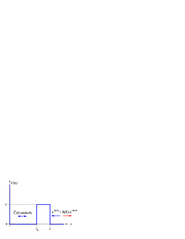
Figure 10: Sketch for the problem of the 1D scattering on a potential given by Eq. (3.253) with the incident wave coming from the right. The internal wave function is given by Eq. (3.256).

We turn now to the question of the temporal evolution of a quantum system, which exhibits a resonance behaviour. Consider an example of the particle motion restricted to a right half-space ($z>0$) with a rectangular barrier of the height $U$ between $z=l_{\rm R}$ and $z=l$.

$$U(z)=\left\{\begin{array}[]{lll}\infty&,&z\leq 0\\ 0&,&0<z<l_{\rm R}\\ U&,&l_{\rm R}\leq z\leq l\\ 0&,&l<z\,.\end{array}\right.$$ (3.253)

We start this section assuming that $E<U$, so that the classical motion is possible for $0<z<l_{\rm R}$ and $z>l$, and for $l_{\rm R}<z<l$ we deal with the tunneling. Applying the results of Sect. 3.1 we may use the wave function (3.104) for $z\geq 0$ and identify $l=L/2$. The internal wave function [Eq. (3.116)] contains only the anti-symmetric part

$$\psi_{U}(z,E) = \widetilde{C}_{-}(E)\,\chi_{-}(z,E)\,,$$

$$\chi_{-}(z,E) = \left\{\begin{array}[]{lll}\sin(k\,z/\hbar)&,&0\leq z<l_{\rm R}\\ \sin(k\,l_{\rm R}/\hbar)\cosh\big{(}\varkappa(z-l_{\rm R})/\hbar\big{)}+\frac{k}{\varkappa}\cos(k\,l_{\rm R}/\hbar)\sinh\big{(}\varkappa(z-l_{\rm R})/\hbar\big{)}&,&l_{\rm R}\leq z\leq l\end{array}\right.\,,$$ (3.256)

where, as before, $k=\sqrt{2mE}$ and $\varkappa=\sqrt{2m(U-E)}$. The logarithmic derivative is equal to

$$d_{-}(E) = l\frac{{\rm d}}{{\rm d}z}\log\chi_{-}(z,E)\Big{|}_{z=l}=\frac{l\varkappa}{\hbar}\frac{k+\varkappa\tan(k\,l_{\rm R}/\hbar)\tanh\big{(}\varkappa(l-l_{\rm R})/\hbar\big{)}}{k\,\tanh\big{(}\varkappa(l-l_{\rm R})/\hbar\big{)}+\varkappa\tan(k\,l_{\rm R}/\hbar)}$$ (3.257)

$$= \frac{l\varkappa}{\hbar}\,\frac{\zeta(E,l_{\rm R})+\mathfrak{p}(E)}{\zeta(E,l_{\rm R})-\mathfrak{p}(E)}\,,$$

where we denoted

$$\zeta(E,l_{\rm R})=\frac{k\cot(k\,l_{\rm R}/\hbar)+\varkappa}{k\cot(k\,l_{\rm R}/\hbar)-\varkappa}\,,\quad\mathfrak{p}(E)=e^{-2\varkappa(l-l_{\rm R})/\hbar}\,.$$ (3.258)

Note that for $l_{\rm R}=0$ we recover from Eq. (3.257) the result of Eq. (3.119) for $d_{-}$. Working within a half-space we have to put $d_{+}\equiv d_{-}$, then from Eqs. (3.109) and (3.110) we find the reflection amplitude

$$R(E) = e^{i\pi-i2\,kl/\hbar}\frac{d_{-}(E)+i\,k\,l/\hbar}{d_{-}(E)-i\,k\,l/\hbar}=e^{i\phi_{\rm R}(E)}\,,\quad\phi_{\rm R}(E)=\pi-2kl/\hbar+\delta_{\rm s}(E)\,,$$ (3.259)

with the scattering phase $\delta_{\rm s}$ given by the relation

$$e^{i\delta_{\rm s}(E)}=\frac{\varkappa+i\,k}{\varkappa-i\,k}\,\frac{\zeta(E,l_{\rm R})+\frac{\varkappa-i\,k}{\varkappa+i\,k}\,\mathfrak{p}(E)}{\zeta(E,l_{\rm R})+\frac{\varkappa+i\,k}{\varkappa-i\,k}\,\mathfrak{p}(E)}\,.$$ (3.260)

The coefficient $\widetilde{C}_{-}(E)$ of the internal wave function defined in Eqs. (3.114) and  (3.116) can be expressed with the help of Eq. (3.257) and the relation

$$\chi_{-}(l,E)=\frac{\sin(kl_{\rm R}/\hbar)}{\sqrt{\mathfrak{p}(E)}}\frac{\zeta(E,l_{\rm R})-\mathfrak{p}(E)}{\zeta(E,l_{\rm R})-1}$$

following from Eq. (3.256) as

$$\widetilde{C}_{-}(E) = \frac{2\,i\sqrt{\mathfrak{p}(E)}}{\sin(k\,l_{\rm R}/\hbar)}\frac{k\,e^{-ikl/\hbar}}{\varkappa-ik}\frac{1-\zeta(E,l_{\rm R})}{\zeta(E,l_{\rm R})+\frac{\varkappa+i\,k}{\varkappa-i\,k}\mathfrak{p}(E)}$$ (3.261)

$$= 2\,i\sqrt{\mathfrak{p}\frac{k^{2}\,(\zeta-1)^{2}+\varkappa^{2}\,(\zeta+1)^{2}}{k^{2}\,(\zeta-\mathfrak{p})^{2}+\varkappa^{2}\,(\zeta+\mathfrak{p})^{2}}}\,e^{i\pi-ikl/\hbar+i\delta_{\rm s}(E)/2}\,.$$

In the last equation we used explicitly that $E<U$ and $\varkappa$ is real, and we suppressed the arguments of functions $\zeta$ and $\mathfrak{p}$ for shortness. We also used that $1/\sin^{2}(k\,l_{\rm R})=1+(\varkappa^{2}/k^{2})(\zeta+1)^{2}/(\zeta-1)^{2}$.

If $U>U^{(n)}=\pi\,\hbar^{2}(2\,n+1)/(4\,m\,l_{\rm R}^{2})$, equation $\zeta(E,l_{\rm R})=0$ has $n$ solutions, $\{\varepsilon_{i}\}$, $i=1,\dots,n$, which constitute the spectrum of bound states for the rectangular potential well (3.253), provided we put $l\to\infty$. For energies close to $\varepsilon_{i}$ we can expand $\zeta(E,l_{\rm R})\approx r_{\zeta,i}(E-\varepsilon_{i})/4\,\varepsilon_{i}$, where $r_{\zeta,i}=(l_{\rm R}\,\varkappa_{i}/\hbar+1)(k_{i}^{2}/\varkappa^{2}_{i}+1)$, $k_{i}=\sqrt{2m\varepsilon_{i}}$, and $\varkappa_{i}=\sqrt{2m(U-\varepsilon_{i})}$. Hence, the amplitude $R(E)$ possesses simple poles at energies $E_{i}$.

Consider the case of a broad barrier. Then $\mathfrak{p}(\epsilon_{i})\ll 1$, and the poles are close to $\varepsilon_{i}$,

$$E_{i} = \varepsilon_{i}-\frac{4\,\varepsilon_{i}}{r_{\zeta,i}}\frac{\varkappa_{i}+i\,k_{i}}{\varkappa_{i}-i\,k_{i}}\,\mathfrak{p}(\varepsilon_{i})=E_{{\rm R},i}-\frac{i}{2}\Gamma_{i}\,,$$ (3.262)

with the real, $E_{{\rm R},i}$ and imaginary, $-\Gamma_{i}/2$, parts, given by

$$E_{{\rm R},i} = \varepsilon_{i}-\frac{4\,\varepsilon_{i}}{r_{\zeta,i}}\frac{\varkappa_{i}^{2}-k_{i}^{2}}{\varkappa_{i}^{2}+k_{i}^{2}}\,\mathfrak{p}(\varepsilon_{i})\,,\quad\Gamma_{i}=\frac{16\,\varkappa_{i}^{2}k^{2}_{i}}{(\varkappa_{i}^{2}+k_{i}^{2})^{2}}\mathfrak{p}(\varepsilon_{i})\frac{\varkappa_{i}k_{i}}{2m(l_{\rm R}\varkappa_{i}/\hbar+1)}\,.$$ (3.263)

Expression for the width $\Gamma_{i}$ has a simple semiclassical interpretation: $\Gamma_{i}=\hbar\,|T(E_{{\rm R},i})|^{2}/P(E_{{\rm R},i})$ , where in the limit $\varkappa(l-l_{\rm R})/\hbar\gg 1$, which we now consider, $|T|^{2}$ is the transmission coefficient of the barrier, cf. Eq. (3.121), and $P=2(m/k)(l_{\rm R}+\hbar/\varkappa)$ is the period of the particle motion within the potential well ($0<z<l_{\rm R}$). The latter expression takes into account that the particle can enter a depth $\hbar/\varkappa$ under the barrier. In other words the width is given by the product of the number of hits of the particle off the barrier per unit of time and the probability of the barrier penetration after each collision. This result survives for arbitrary barrier within applicability of semiclassical approximation [7]. Close to the resonance, $E\sim E_{{\rm R},i}$, the amplitude can be written as

$$R(E)\approx e^{i\pi-2i\,k_{i}l/\hbar+2i\beta_{\varkappa}(\varepsilon_{i})}\frac{E-E_{{\rm R},i}-\frac{i}{2}\Gamma_{i}}{E-E_{{\rm R},i}+\frac{i}{2}\Gamma_{i}}\approx e^{i\pi-2\,i\,k_{i}l/\hbar+2i\beta_{\varkappa}(E)+2\,i\,\delta_{i}(E)}\,.$$ (3.264)

We see that the phase shift can be approximately presented as $\delta_{\rm s}(E)\approx 2\beta_{\varkappa}(E)+2\delta_{i}(E)$, where the resonance scattering phase is given by

$$\delta_{i}(E)=\arctan\Big{(}\frac{\Gamma_{i}/2}{E_{{\rm R},i}-E}\Big{)}\,,$$ (3.265)

and the non-resonant (potential) phase $\beta_{\varkappa}$ is defined by Eq. (3.230). Note that the values $E_{{\rm R},i}/\hbar$ and $\Gamma_{i}/\hbar$ here have the same meaning as the values $\omega_{\rm R}$ and $\Gamma$, which we used in Sect. 2, cf. poles of the Green’s functions (2.30) and Eq. (3.262).

For the case $\Gamma_{i}\ll|E_{{\rm R},i+1}-E_{{\rm R},i}|$, which we will further consider, we can write

$$R(E)\approx\sum_{i=1}^{n}e^{-2\,ik_{i}l/\hbar+i\beta_{\varkappa}(E)}\frac{i\Gamma_{i}}{E-E_{{\rm R},i}+\frac{i}{2}\Gamma_{i}}\,.$$ (3.266)

Consider now the temporal aspects of this scattering problem. Defining the dwell time in the same way as in Sect. 3.2, after some manipulations we obtain with the help of Eqs. (3.256) and (3.261)

$$t_{\rm d}(0,l,E) = \frac{1}{v}\intop_{0}^{l}|\psi_{U}(z,E)|^{2}{\rm d}z=\frac{m}{k}\mathfrak{p}\frac{k^{2}+\varkappa^{2}}{k^{2}\,[\zeta-\mathfrak{p}]^{2}+\varkappa^{2}\,[\zeta+\mathfrak{p}]^{2}}$$ (3.267)

$$\times\Big{(}2\,l_{\rm R}(\zeta+1)^{2}-\frac{8l_{\rm R}\zeta k^{2}}{k^{2}+\varkappa^{2}}+\frac{2\hbar}{\varkappa}\Big{[}(1-\zeta^{2})+\frac{k^{2}}{k^{2}+\varkappa^{2}}\,\big{(}2\zeta\log\mathfrak{p}+\zeta^{2}/\mathfrak{p}-\mathfrak{p}\big{)}\Big{]}\Big{)}\,.$$

The value $t_{\rm d}(0,l,E)$ is the time needed by the incident current $j_{\rm I}=v=k/m$ to fill the internal region $[0,l]$ with the probability density $|\psi_{U}(z,E)|^{2}$. The quantity (3.267) is plotted in Fig. 11 as a function of the energy for different barrier penetrabilities parameterized through the value $\mathfrak{p}(E)=\exp(\sqrt{1-E/U}\log\mathfrak{p}(0))$ at the zero energy. For a tiny barrier penetrability the internal wave function has a small amplitude for most energies $\propto|\widetilde{C}_{-}|\propto\mathfrak{p}\ll 1$ and therefore the dwell time is very short. Only for the energies close to the resonance $\zeta\sim\mathfrak{p}$ the internal wave function can acquire a large amplitude $|\widetilde{C}_{-}|\propto 1/\mathfrak{p}$ and the dwell time becomes very large. Exactly at the resonance energy, $E=E_{{\rm R},i}$, we find that

$$t_{\rm d}(0,l,E_{{\rm R},i})\approx\frac{4\hbar}{\Gamma_{i}}\,,$$ (3.268)

where we used that $\zeta(E_{{\rm R},i})=-\mathfrak{p}(\varkappa_{i}^{2}-k_{i}^{2})/(\varkappa_{i}^{2}+k_{i}^{2})$ as follows from Eq. (3.263). By varying the length of the resonator $l_{\rm R}$ one can change the number of resonances in the potential, see different panels in Fig. 11 plotted for different values of $l_{\rm R}$.

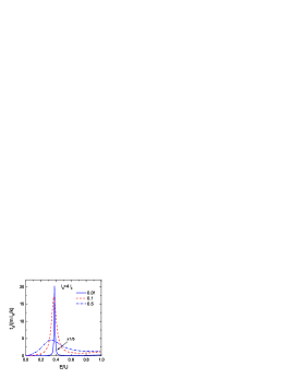
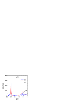
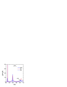
Figure 11: The dwell time (3.267) for the potential (3.253) as a function of the energy for various values of the coefficient $\mathfrak{p}(0)$, see Eq. (3.258), shown by the line labels. Three panels demonstrate results for various values of $l_{\rm R}$ measured in units $l_{0}=\hbar/\sqrt{2mU}$. The solid lines in all panels are multiplied by factor $1/5$.

Describing the scattering problem in terms of the wave packet (3.143) collected now with the wave function (3.104) with $T=0$, $R$ given by Eq. (3.259) and the internal function (3.256), we can define the reflection group time in the same way as in Sect. 3.4: This is the time interval between the moment, when the maximum of the incident wave packet moving towards the origin is at the position $z=l$ and the moment, when the maximum of the reflected packet moving away from the potential region is at the same position $z=l$. Applying this definition to a wave-packet with the energy distribution $\Phi(E)$ sharply peaked at the averaged energy $\overline{E}$ with a small energy spread $\gamma$, $\gamma\ll\Gamma_{i}$, we find

$$t_{\rm R}(\overline{E})=2\frac{l}{\widetilde{v}}+\hbar\frac{{\rm d}\phi_{\rm R}(\overline{E})}{{\rm d}\overline{E}}=\hbar\frac{{\rm d}\delta_{\rm s}(\overline{E})}{{\rm d}\overline{E}}\,,$$ (3.269)

where $\overline{E}\equiv m\widetilde{v}^{2}/2$. The physical meaning of the quantity $t_{\rm R}$ is the following: If we send a wave packet with the well-defined energy $\overline{E}$ and observe the reflected packet at a fixed distance $z$ from the scattering centre, $z\gg l$, then $t_{\rm R}(\overline{E})$ is the time delay in the arrival of the emitted wave packet with respect to the case without barrier. For energies close to the resonant ones $\overline{E}\sim E_{{\rm R},i}$ and $\Gamma_{i}\ll|E_{{\rm R},i+1}-E_{{\rm R},i}|$ the reflection group time can be written as

$$t_{\rm R}(\overline{E})\approx-2\frac{l_{\rm R}}{\widetilde{v}}+\sum_{i}2\hbar\frac{{\rm d}\delta_{i}(\overline{E})}{{\rm d}\overline{E}}=-2\frac{l_{\rm R}}{\widetilde{v}}+\sum_{i}\frac{\hbar\Gamma_{i}}{(\overline{E}-E_{{\rm R},i})^{2}+{\textstyle\frac{1}{4}}\Gamma_{i}^{2}}\,.$$ (3.270)

We used that for $\overline{E}$ close to $E_{{\rm R},i}\simeq\varepsilon_{i}$ we have $\beta_{\varkappa}(\overline{E})\simeq\arctan(k_{i}/\varkappa_{i})=-k_{i}l_{\rm R}/\hbar\simeq-\widetilde{k}l_{\rm R}/\hbar$ with $\widetilde{k}=\sqrt{2m\overline{E}}$. We see that, if $\overline{E}=E_{{\rm R},i}$, then the resonance time delay is as large as

$$t_{\rm R}(E_{{\rm R},i})\approx\frac{4\hbar}{\Gamma_{i}}\,.$$ (3.271)

Hence, the incident wave packet lingers in the interaction region much longer than if it crossed this distance with the mean velocity. If the particle energy is de-tuned from any resonance $|\overline{E}-E_{{\rm R},i}|\gg\Gamma_{i}$, then $t_{\rm R}$ changes the sign and we deal with the time advancement

$$t_{\rm R}\approx-2\frac{l_{\rm R}}{\widetilde{v}},$$ (3.272)

as for classical scattering on a hard sphere, cf. Eq. (2.83). As we see, the internal part of the potential $0<z<l_{\rm R}$ is effectively excluded from the particle motion. Interestingly, in Eq. (3.272) there is no contribution from the under-barrier region $[l_{\rm R},l]$. It seems like the packet instantly passes under barrier but does not enter the resonator $[0,l_{\rm R}]$. This is a manifestation of the Hartman phenomenon discussed in Sect. 3.6. In this connection we have to emphasize that the group time $t_{\rm R}$ is not a proper measure of the time the tunneling particle spends under the barrier.

The dwell time (3.267) and the reflection group time (3.269) are connected by the relation similar to Eq. (3.167) following from Eq. (2.505):

$$t_{\rm d}(0,l,\overline{E})=t_{\rm R}(\overline{E})-\delta t_{\rm i}(\overline{E}),$$ (3.273)

where the interference time delay is given by

$$\delta t_{\rm i}(\overline{E})=-\frac{\hbar}{\widetilde{k}\widetilde{v}}\sin\big{(}2\,k\,l+\phi_{\rm R}(\overline{E})\big{)}=\frac{\hbar}{2\overline{E}}\sin\delta_{\rm s}(\overline{E})\,.$$ (3.274)

Close to the resonance energy the interference time is not singular, vanishing at $\overline{E}=E_{{\rm R},i}$, and is much smaller than the reflection group time $t_{\rm R}$ and the dwell time $t_{\rm d}$.

Since, as depicted in Fig. 10, there is obvious symmetry in the motion of a particle towards the origin and away from it, it is convenient to define a measure of time for a reflected wave only. Then we define the scattering group time,

$$t_{\rm s}(\overline{E})=\frac{1}{2}t_{\rm R}(\overline{E}),$$ (3.275)

as a half of the bidirectional scattering time defined in Eq. (3.164), $t_{\rm s}=t_{\rm bs}/2$. The time $t_{\rm s}$ corresponds to the group time defined for the classical motion in Eq. (2.11). The similar time quantity is introduced in Eq. (2.84) for classical particles undergoing the scattering on a hard sphere. In view of the relation (3.273) it is convenient to introduce also the single-way dwell time

$${t}_{\rm d}^{\rm s.w.}(0,l,\overline{E})=\frac{1}{2}t_{\rm d}(0,l,\overline{E}),$$ (3.276)

so that close to the resonance energy for a narrow resonance we have

$$t_{\rm s}(\overline{E})\approx{t}_{\rm d}^{\rm s.w.}(0,l,\overline{E})\approx\sum_{i=1}^{n}\hbar\frac{{\rm d}\delta_{i}(\overline{E})}{{\rm d}\overline{E}}=\sum_{i=1}^{n}\frac{\hbar\Gamma_{i}/2}{(\overline{E}-E_{{\rm R},i})^{2}+{\textstyle\frac{1}{4}}\Gamma_{i}^{2}}\equiv\sum_{i=1}^{n}\frac{\hbar}{2}A_{i}(\overline{E})\,.$$ (3.277)

Each of the functions $A_{i}(\overline{E})$ satisfies the sum rule

$$\int_{-\infty}^{\infty}A_{i}(E)\frac{{\rm d}E}{2\pi}=1,$$ (3.278)

cf. Eqs. (2.67), (2.68), (2.69) in classical mechanics. Here the integral sits near each $i$-th pole and thereby we are able to perform integration from $-\infty$ to $\infty$ or from $0$ to $\infty$. Correspondingly, the integral over the energy of the scattering group time or the single-way dwell time yield the number of resonances in the system

$$\int_{0}^{\infty}t_{\rm s}(E)\frac{{\rm d}E}{\pi\hbar}\approx\int_{0}^{\infty}{t}_{\rm d}^{\rm s.w.}(0,l,E)\frac{{\rm d}E}{\pi\hbar}\approx n\,.$$ (3.279)

Thus the dwell time defined in Eq. (3.267) can be related to the number of states per unit energy

$$t_{\rm d}(0,l,E)=2{t}_{\rm d}^{\rm s.w.}(0,l,E)\approx 2\pi\hbar\frac{{\rm d}n}{{\rm d}E}\,,$$ (3.280)

cf. the semiclassical relation (3.132).

We turn now to a more detailed study of the wave function of the scattering problem with the potential (3.253). For the sake of further applications let us now re-organize the wave functions of the stationary problem shown in Fig. 10 to deal with the incident and reflected currents equal to unity outside the barrier. For this we multiply the wave function (3.104) with $R$ given by Eq. (3.259) and the internal wave function (3.256) with the coefficient (3.261) by the factor $i\sqrt{1/v}e^{ik\,l/\hbar-i\delta_{s}(E)/2}$ and obtain

$$\psi(z;E)=\left\{\begin{array}[]{lll}\frac{i}{\sqrt{v}}e^{ik\,l/\hbar-i\delta_{\rm s}(E)/2}\widetilde{C}_{-}(E)\chi_{-}(z,E)&,&z\leq l\\ \sqrt{\frac{4}{v}}\sin(k\,(z-l)/\hbar+\delta_{\rm s}(E)/2)&,&z>l\end{array}\right.\,\,,$$ (3.283)

Expressions for $\widetilde{C}_{-}(E)$ and $\delta_{s}(E)$ were derived above for $E<U$. For $E>U$ the coefficient $\widetilde{C}_{-}(E)$ is given by the first line in Eq. (3.261) and the phase $\delta_{\rm s}(E)$ is defined in Eq. (3.260) after the replacement $\varkappa\to i|\varkappa|$, there and in Eq. (3.258). The wave functions (3.283) are normalized as

$$\intop_{0}^{\infty}\psi^{*}(z,E)\,\psi(z,E^{\prime})\,{\rm d}z=2\pi\hbar\,\delta(E-E^{\prime})\,.$$ (3.284)

For our further study of the time evolution of a quantum system such a normalization is more convenient than that given by Eq. (3.144).

If we deal with a system with narrow and isolated resonances, i.e. we assume that the potential barrier is broad, $\mathfrak{p}\ll 1$, and the resonator length $l_{\rm R}$ is such that $|E_{{\rm R},i+1}-E_{{\rm R},i}|\gg\Gamma_{i}+\Gamma_{i+1}$, the internal wave function acquires for $E<U$ a sizable magnitude only, if the energy $E$ is close to the resonance one. In the vicinity of the $i$-th resonance $E\sim E_{{\rm R},i}$, we may put $\sin(k_{i}l_{\rm R}/\hbar)=k_{i}/\sqrt{\varkappa_{i}^{2}+k_{i}^{2}}$ in Eq. (3.261) and it takes the form

$$\widetilde{C}_{-}(E) \approx 2\,i\frac{4\varkappa_{i}^{2}\,\varepsilon_{i}\,e^{-\varkappa(l-l_{\rm R})/\hbar}}{(k_{i}^{2}+\varkappa_{i}^{2})(l_{\rm R}\varkappa_{i}/\hbar+1)}\frac{e^{-i\,k_{i}\,l/\hbar+i\beta_{\varkappa}(E)}}{E-E_{{\rm R},i}+\frac{i}{2}\Gamma_{i}}$$ (3.285)

$$\approx -i\sqrt{\frac{2\,v}{l_{\rm R}}}e^{-i\,k\,l/\hbar+i\beta_{\varkappa}(E)+i\delta_{i}(E)}\sqrt{\frac{\hbar\Gamma_{i}}{(E-E_{{\rm R},i})^{2}+\Gamma_{i}^{2}/4}}.$$

Taking this into account the internal part of the wave function can be written for $E<U$ as follows

$$\psi(z\leq l;E<U)\approx\sum_{i=1}^{n}\sqrt{\frac{\hbar\,\Gamma_{i}}{(E-E_{{\rm R},i})^{2}+\Gamma_{i}^{2}/4}}\,\sqrt{\frac{2}{l_{\rm R}}}\chi_{-}(z,E)\,,\quad z\leq l\,,$$ (3.286)

where each element of the sum contributes only fort $|E-E_{{\rm R},i}|\ll|E_{{\rm R},i+1}-E_{{\rm R},i}|$ . This expression shows that only the particles with energies within the interval $E_{{\rm R},i}-\Gamma/2<E<E_{{\rm R},i}+\Gamma/2$ penetrate inwards through the barrier and from the internal wave function.

The wave function in Eq. (3.286) allows for the important generalization. The coordinate part of the internal wave function can be replaced by the stationary wave function of the closed quantum system, which is obtained from those shown in Fig. 10 by extending the barrier to infinity, $l\to\infty$. Herewith the $n$ resonance states at energies $E_{{\rm R},i}$ (with the widths $\Gamma_{i}$) turn into $n$ bound states with energies $\varepsilon_{i}$ with the wave functions

$$\psi^{\rm(bound)}_{i}(z)=C_{i}\chi_{-}(z,\varepsilon_{i})\,.$$ (3.287)

Since the barrier was initially broad, $\Gamma_{i}$ being small, and the difference between the energy of the bound state and the energy of the resonance is small $|{\varepsilon}_{i}-E_{\rm R,i}|=O\big{(}\mathfrak{p}(E_{\rm R,i})\big{)}$. Similarly the normalization coefficients $C_{i}$ differ from $\sqrt{2/l_{\rm R}}$ by a small factor $O\big{(}\mathfrak{p}(E_{\rm R,i})\big{)}$. Then $\psi(z;E<U)$ in (3.286) is factorized as

$$\psi(z;E<U)\approx\sum_{i=1}^{n}\sqrt{A_{i}(E)}\psi^{\rm(bound)}_{i}(z)\,.$$

Such a factorization of the internal wave function of a scattering problem into a wave function of the corresponding bound state problem and an enhancement factor $\sqrt{A_{i}(E)}$ is argued in Refs. [97, 98, 99, 79] to be possible for any finite-range potential and with some modifications also for the Coulomb potential. These results have found applications in the studies of nucleon-halo nuclei [100] and di-proton radioactivity [97, 101].

With the help of the wave functions (3.286) we can give a new interpretation for the dwell time $t_{\rm d}^{\rm s.w.}(0,l,E)$. It can be presented as the ratio of the density of states in the region of the potential to the density of the free states in the same region (i.e. the relative probability for the particle to be inside the region of the potential compared to the scattering in the absence of the potential) multiplied by the time of the free motion inside the potential region $l/v$:

$$t_{\rm d}^{\rm s.w.}(0,l,E)=\hbar\frac{l}{v}\frac{\int_{0}^{l}|\psi(z;E)|^{2}{\rm d}z}{\int_{0}^{l}|\psi^{\rm(free)}(z;E)|^{2}{\rm d}z}\,,\quad\psi^{\rm(free)}(z;E)=\sqrt{\frac{4}{v}}\sin(k\,z/\hbar)\,.$$ (3.288)

This is in accord with the ergodicity principle, see below Sect. 4.4.1.

Now consider the problem of the decay of quasistationary states. The problem can be formulated as follows. Assume that one sends a stationary particle flux of the energy $E_{1}$ on the potential shown in Fig. 10, and we ask the question how long particles from the beam will be delayed inside the region of the potential ($0<z<l_{\rm R}$) in dependence of the value $E_{1}$ of beam energy after the beam was suddenly switched off. Particles from the beams having real energies $E_{1}$ within bands, $E_{{\rm R},i}\pm\alpha\Gamma_{i}$, $\alpha\sim 1$, form wave packets, corresponding to initial (after switching off the beam) quasistationary states, which leave long inside the potential well (if the barrier is broad) till the particles describing by these distributions penetrate through the barrier to infinity. The particles with initial beam energies far from energies $E_{{\rm R},i}\pm\alpha\Gamma_{i}$ enter the region of the potential well only with a tiny probability. So, we may address the question how long a particle corresponding the initial real energy $E_{1}$ from the band $E_{{\rm R},i}\pm\alpha\Gamma_{i}$ (or, better to say, particles corresponding to an energy distribution within the band provided the beam had a finite energy dispersion)) stays in the resonance quasistationary state till its decay? (The question how long does it take for the particle to pass the barrier has been considered above.) One can prepare, of course, a more complicated quasistationary states by populating not one but several resonant states using the incident wave packet with a broader energy distribution.

A similar initial state can be prepared differently. The initial localized state can be created right inside the potential well (for $0<z<l_{\rm R}$), e.g. by reactions. If the barrier is broad, at times much shorter than the decay times of the resulting quasistationary states the produced particles with $E<{\rm max}\,\,U$ are redistributed over the energy levels corresponding to the stationary levels related to the same problem but with not penetrable barrier. On a longer time scale each of these levels is actually a quasistationary level and our problem is to find the decay time.

Considering a general case, we assume that at the time $t=0$ our system is described by an arbitrary wave function $\Psi(z,0)$ localized inside the potential region, i.e we assume $\Psi(z,0)=0$ for $z>l_{\rm R}$. The evolution of this state is determined by the unitary operator $\exp(-i\,\hat{H}t)$, so that at any later time $t>0$ the wave function of the system is equal to $\Psi(z,t)=\exp(-i\,\hat{H}t)\Psi(z,0)$. Expanding the initial wave function in terms of the eigenfunctions of the Hamiltonian $\hat{H}$, ${\psi}(z;E)$ for $E>0$, normalized as in Eq. (3.284) we can write

$$\Psi(z,t)=\int_{0}^{\infty}\frac{{\rm d}E}{2\pi\hbar}\Phi(E)\,\psi(z;E)e^{-iEt/\hbar},$$ (3.289)

where

$$\Phi(E)=\int_{0}^{\infty}{\rm d}z\psi^{*}(z;E)\Psi(z,0)=\int_{0}^{l}{\rm d}z\psi^{*}(z;E)\Psi(z,0)\,.$$ (3.290)

The unitary evolution conserves the normalization of the wave function and since the initial wave function is normalized to unity, then

$$\int_{0}^{\infty}dz|\Psi(z,t)|^{2}=\int_{0}^{l}dz|\Psi(z,0)|^{2}=\int_{0}^{\infty}\frac{{\rm d}E}{2\pi\hbar}|\Phi(E)|^{2}=1$$ (3.291)

for any moment of time $t$. Note the difference in normalization of the function $\Phi(E)$ in comparison with Eq. (3.145).

The overlap between the wave function at time $t$ and the initial wave function gives the amplitude of the survival probability (also called integrity)

$$\mathcal{G}(t)=\int_{0}^{\infty}\Psi^{*}(z,0)\Psi(z,t){\rm d}z=\int_{0}^{\infty}\frac{{\rm d}E}{2\pi\hbar}|\Phi(E)|^{2}e^{-iEt/\hbar},$$ (3.292)

so that $\mathcal{P}_{\rm surv}(t)=|\mathcal{G}(t)|^{2}$ is the probability that the system remains in the same state after passage of time $t$. Obviously at $t=0$ probability $\mathcal{P}_{\rm surv}$ is equal to unity, $\mathcal{G}(0)=1$ in view of Eq. (3.291). At any later time it becomes smaller than unity, as follows from the Cauchy-Schwarz-Bunyakovsky inequality

$$|\mathcal{G}(t)|=\Big{|}\int_{0}^{\infty}\Psi^{*}(z,0)\Psi(z,t){\rm d}z\Big{|}\leq\Big{|}\int_{0}^{\infty}|\Psi(z,0)|^{2}{\rm d}z\Big{|}^{1/2}\Big{|}\int_{0}^{\infty}|\Psi(z,t)|^{2}{\rm d}z\Big{|}^{1/2}=1\,.$$ (3.293)

Since the function $|\Phi(E)|^{2}$ is integrable on the ray $[0,+\infty)$, see Eq. (3.291), one can prove [102] that $\lim_{t\to\infty}\mathcal{G}(t)=0.$ This means that an initial state will always decay at large times. Under the assumption of a purely exponential decay one identifies the lifetime of the system in the initial state, or its decay time, as $t_{\rm dec}=-\mathcal{P}_{\rm surv}(t)/\dot{\mathcal{P}}_{\rm surv}(t)$, which in this case would be a time-independent quantity. However Khalfin in Ref. [103] pointed out that $\mathcal{P}_{\rm surv}(t)$ cannot be purely exponential. It deviates from the exponent both for very large times and for very short times. This conclusion is obtained without any assumptions about the quantum state and the system dynamics. For more extensive discussion of this issue we address the reader to the review [65]. Possible manifestations of a non-exponential decay in nuclear systems are discussed, e.g., in [104]. Peculiarities of a many-body quantum decay are studied in [105], where important role of effects of the quantum statistics is demonstrated.

Since, as argued above, the purely exponential decay is not possible for all times, it would be desirable to find such a definition of the decay time, which does not depend on the assumption of a particular form of the survival probability amplitude. Following Fleming [106] let us define the decay time of the unstable state as

$$t_{\rm dec}=\intop_{0}^{\infty}{\rm d}t|\mathcal{G}(t)|^{2}\,=\frac{1}{2}\intop_{0}^{\infty}\frac{{\rm d}E}{2\pi\hbar}|\Phi(E)|^{4}\,,$$ (3.294)

where we used Eq. (3.292). The integral exists, if $|\mathcal{G}(t)|^{2}\lesssim 1/t^{1+\delta}$ for large $t$. The sojourn time

$$t_{\rm soj}(0,l)=\intop_{0}^{\infty}{\rm d}t\intop_{0}^{l}{\rm d}z|\Psi(z,t)|^{2}\,$$ (3.295)

is a characteristic of how long the particle stays within interval $[0,l]$ starting from initial moment $t=0$, see Eq. (3.180). By analogy to Eq. (3.181) we can express the sojourn time through the dwell time (3.267) averaged with $|\Phi(E)|^{2}$ over the energy

$$t_{\rm soj}(0,l)=\frac{1}{2}\int_{0}^{\infty}\frac{{\rm d}E}{2\pi\hbar}|\Phi(E)|^{2}\,\intop_{0}^{l}{\rm d}z|{\psi}(z;E)|^{2}=\frac{1}{2}\intop_{0}^{\infty}\frac{{\rm d}E}{2\pi\hbar}|\Phi(E)|^{2}t_{\rm d}(0,l,E)\,.$$ (3.296)

Here in the last equation we take into account the different normalization of the wave function $\psi_{U}$ used in Eq. (3.267) and the wave function $\psi$, Eq. (3.286) used in the expansion (3.289), which produces the factor $1/v$ needed in Eq. (3.267).

Let us now illustrate how the above formulae work for the case of very narrow isolated resonances. The preparation of the initial wave function $\Psi(z,0)$ for such a quasistationary states can be done by putting infinite wall somewhere inside the barrier or one can use the simple method of Refs. [79]: in the potential (3.253) we extend the barrier to infinity by putting $l\to\infty$. In the latter case we can expand initial localized wave function in terms of the wave functions (3.287) as

$$\Psi(z,0)=\sum_{i}^{n}c_{i}\psi^{\rm(bound)}_{i}(z)+\int_{U}^{\infty}\frac{{\rm d}E}{2\pi\hbar}\tilde{c}(E)\,\psi(z,E)\,,\quad\sum_{i=1}^{n}|c_{i}|^{2}+\int_{U}^{\infty}\frac{{\rm d}E}{2\pi\hbar}|\tilde{c}(E)|^{2}=1\,.$$ (3.297)

The wave function under the integral is given by Eq. (3.283) for $E>U$. If we now suddenly recover initial form of the potential (in the time $\ll\hbar/\min(|\varepsilon_{i}-\varepsilon_{i+1}|)$ for $i<n$) then the wave function does not change and we can substitute it in Eq. (3.290), and using the wave functions (3.283) and (3.286) obtain

$$\Phi(E)\approx\sum_{i}^{n}c_{i}\,\sqrt{\hbar A_{i}(E)}+\overline{\Phi}(E)\,\theta(E-U)\,,$$ (3.298)

where the part $\overline{\Phi}(E)$ corresponds to the modes over the barrier, which do not contribute to the resonant scattering and can be dropped thereby.

For simplicity let us now assume that the initial wave function corresponds to only one $j$-th bound state with $1<j<n$. We have ${c}_{i}=\delta_{ij}$ and $\tilde{c}(E>U)=0$, and $|\Phi(E)|^{2}\approx\hbar A_{j}(E)$. Since close to the resonance energy the dwell time is $t_{\rm d}(0,l,E)\approx\hbar A_{j}(E)$, we find

$$t_{\rm dec} \approx t_{\rm soj}(0,l)\approx\frac{1}{2}\intop_{0}^{\infty}\frac{{\rm d}E}{2\pi}\frac{\hbar\,\Gamma_{j}^{2}}{\big{(}(E-E_{{\rm R},j})^{2}+\Gamma_{j}^{2}/4\big{)}^{2}}\approx\frac{1}{2}\intop_{-\infty}^{\infty}\frac{{\rm d}E}{2\pi}\frac{\hbar\,\Gamma_{j}^{2}}{\big{(}(E-E_{{\rm R},j})^{2}+\Gamma_{j}^{2}/4\big{)}^{2}}=\frac{\hbar}{\Gamma_{j}}.$$ (3.299)

Here we used that for $E_{{\rm R},j}\gg\Gamma_{j}$ the lower limit of the integration can be extended to $-\infty$. Hence, the particles occupied at $t=0$ a narrow quasistationary state with the width $\Gamma$, will appear with the probability of the order of one to the right from the barrier after passing of time $\hbar/\Gamma$. Compare it with Eq. (2.27) introduced in classical mechanics in Sect. 2.

The explicit form of the survival probability amplitude follows from Eq. (3.292):

$$\mathcal{G}(t)=\int_{0}^{\infty}A_{j}(E)e^{-iEt/\hbar}\frac{{\rm d}E}{2\pi\hbar}=e^{-iE_{{\rm R},j}t/\hbar-\Gamma_{j}\,t/2\hbar}+\frac{(1-i)}{\sqrt{2}}\int_{0}^{\infty}\frac{\Gamma_{j}e^{-Et/\hbar}\sqrt{E_{{\rm R},j}/E}}{(iE+E_{{\rm R},j})^{2}+\Gamma_{j}^{2}/4}\frac{{\rm d}E}{2\pi}.$$ (3.300)

To get this expression we assumed the energy dependence of the width $\Gamma(E)\simeq\Gamma\sqrt{E_{{\rm R},j}/E}$, as it follows from analysis of the available phase space of the 1D problem at small energies, and rotated the contour of integration to coincide with the imaginary axis. For $t\gg\hbar/E_{{\rm R},j}$ we find

$$\mathcal{G}(t)\simeq e^{-iE_{{\rm R},j}t/\hbar-\Gamma_{j}t/2\hbar}+\frac{(1-i)}{\sqrt{8\pi}}\frac{\Gamma_{j}}{E_{{\rm R},j}}\Big{(}\frac{\hbar}{E_{{\rm R},j}\,t}\Big{)}^{1/2}\,.$$ (3.301)

For times of $t\ll t_{\rm dec}\log\big{(}8\pi\,E^{3}_{{\rm R},j}/\Gamma_{j}^{3}\big{)}$, i.e. almost in the whole time interval of our interest, the second term can be neglected. If we extend integration to $-\infty$ using that $A_{j}(E)$ is the sharp function of $E$ near $E_{{\rm R},j}>0$, we get

$$\mathcal{G}(t)\simeq\int_{-\infty}^{\infty}A_{j}(E)e^{-iEt/\hbar}\frac{{\rm d}E}{2\pi\hbar}\simeq e^{-iE_{{\rm R},j}t/\hbar-\Gamma_{j}t/2\hbar}.$$ (3.302)

Thus, the correction term in (3.300) is fully compensated by the contribution of negative energies.

We see that in case of a decaying system we deal with a packet propagating outwards the resonator with an effective energy distribution given by $A_{j}(E)$. As we argued in Sect. 3.8, the emerging of the packet on the outer side of the barrier cannot last shorter then $\delta t_{\rm var}\sim\hbar/\gamma=t_{\rm dec}^{\gamma}$, see the Mandelstam-Tamm inequality (3.228), where $\gamma$ is the dispersion of the energy distribution. However, for the Lorentz distribution $A_{j}(E)$ (i.e. for $\Gamma_{j}=const$) the dispersion would be infinite. Here we have to remember that the resonance wave functions (3.286) can be used only for energies not far from the resonance one, i.e. for $E\in[E_{{\rm R},j}-\alpha\Gamma_{j},E_{{\rm R},j}+\alpha\Gamma_{j}]$, for $\alpha\Gamma_{j}\ll|E_{{\rm R},j+1}-E_{{\rm R},j}|$. Taking these energy limits into account we can estimate

$$\gamma^{2}\simeq\int_{-\alpha\Gamma_{j}}^{+\alpha\Gamma_{j}}\frac{{\rm d}E}{2\pi\hbar}E^{2}A_{j}(E+E_{{\rm R},j})\Bigg{/}\int_{-\alpha\Gamma_{j}}^{+\alpha\Gamma_{j}}\frac{{\rm d}E}{2\pi\hbar}A_{j}(E+E_{{\rm R},j})=\Gamma_{j}^{2}\frac{\left(2\alpha-\arctan 2\alpha\right)}{4\arctan 2\alpha}.$$ (3.303)

For $\alpha\simeq 3.58$ we get $\gamma\simeq\Gamma_{j}$. The condition $\gamma\simeq\Gamma$ looks rather natural for the description of the wave packet in quasistationary state.

Thus, the probability to find particle outside the barrier becomes essentially non-zero before the maximum of the wave packet (according to the latter’s position one defines the scattering group time) has reached the point $z=l$ with advancement $\sim t^{\gamma}_{\rm dec}\sim\hbar/\Gamma$ (if we put $\gamma\simeq\Gamma$), and the real forward delay time is given by

$$\delta t_{\rm f}=t_{\rm s}-t^{\gamma}_{\rm dec}\,,$$ (3.304)

cf. Eq. (3.229) above. This quantity demonstrates an advance of the formation and decay of the intermediate states forming in the scattering on the potential (3.253) at energies $|E-E_{\rm R}|>\Gamma/2$ and a delay at energies in the vicinity of the resonance, for $|E-E_{\rm R}|<\Gamma/2$.

Considering a scattering of a packet with an energy distribution $\Phi(E)$ on the potential well (3.253), we may introduce the quantity

$$\bar{t}_{\rm s}(\overline{E})=\int\frac{{\rm d}E}{2\pi\hbar}|\Phi(E)|^{2}t_{\rm s}(E)\approx\int\frac{{\rm d}E}{2\pi\hbar}|\Phi(E)|^{2}\frac{\hbar}{2}\,A_{i}(E)\,.$$ (3.305)

Here $|\Phi(E)|^{2}$ is normalized as in Eq. (3.291). For the Gaussian wave packet $|\Phi(E)|^{2}=\sqrt{2\pi\hbar^{2}/\gamma^{2}}\exp(-(E-\overline{E})^{2}/2\gamma^{2})$ in the limit of a narrow energy distribution $\gamma\ll\Gamma$ we derive $\bar{t}_{\rm s}(\overline{E})={t}_{\rm s}(\overline{E})$ and in the opposite limit case of a very broad distribution $\gamma\gg\Gamma$ we get $\bar{t}_{\rm s}(\overline{E})=1/\gamma$. Thus $\delta t_{\rm f}(\bar{E})=\bar{t}_{\rm s}(\overline{E})-1/\gamma$ for $\gamma\ll\Gamma$ and $\delta t_{\rm f}(\overline{E})=0$ at $\gamma\gg\Gamma$, and only for a very specific choice of the energy distribution in the packet (e.g. for a Lorentzian distribution with $\gamma\simeq\Gamma$) we arrive at $\delta t_{\rm f}=\bar{t}_{\rm s}(\bar{E})-1/\Gamma$, as we obtained above for the case of an initially localized state.

It is instructive to rewrite the survival probability amplitude (3.292) in the following form

$$\mathcal{G}(t)=i\int_{0}^{\infty}{\rm d}z\int_{0}^{\infty}{\rm d}z^{\prime}\Psi^{*}(z,0)\,G^{R}(t,z,z^{\prime})\,\Psi(z^{\prime},0)\,,$$ (3.306)

where we introduce the retarded Green’s function $G^{R}(t,z,z^{\prime})$, which describes the evolution of the wave function, $\Psi(z,t)=\intop_{0}^{\infty}{\rm d}z^{\prime}G^{R}(t,z,z^{\prime})\Psi(z,0)$ forward in time, i.e. $G^{R}(t,z,z^{\prime})\equiv 0$ for $t<0$, cf. the same quantity in classical mechanics (2.24), (2.30), and (2.33). The Green’s function is expressed through the eigenfunctions (3.286) and (3.283)

$$G^{R}(t,z,z^{\prime})=\intop_{-\infty}^{\infty}\frac{{\rm d}E}{2\pi}G_{R}(E,z,z^{\prime})e^{-iEt/\hbar}\,,\quad G^{R}(E,z^{\prime},z)=\intop_{0}^{\infty}\frac{{\rm d}E^{\prime}}{2\pi\hbar}\frac{\psi(z;E^{\prime})\,\psi^{*}(z^{\prime};E^{\prime})}{E-E^{\prime}+i0}\,.$$ (3.307)

The small shift of the pole in the last integral in the lower complex semi-plane assures that the Green’s function vanishes for $t<0$, since

$$\theta(t)e^{-iEt/\hbar}=i\int_{-\infty}^{+\infty}\frac{{\rm d}E^{\prime}}{2\pi}\frac{e^{-iE^{\prime}t/\hbar}}{E^{\prime}-E+i0}.$$ (3.308)

For energies $E<U$ and for the case of narrow resonances we can use the wave function of the resonance states (3.286) with the replacement of their coordinate parts by the wave-functions of the corresponding bound states (3.287). Then the coordinate and energy dependence of the Green’s function separate as follows

$$G^{R}(E,z^{\prime},z)\approx\sum_{i=1}^{n}G_{i}^{R}(E)[\psi^{\rm(bound)}_{i}(z^{\prime})]^{*}\,\psi^{\rm(bound)}_{i}(z)\,,$$

$$G_{i}^{R}(E)=\intop_{0}^{\infty}\frac{{\rm d}E^{\prime}}{2\pi}\frac{A_{i}(E)}{E-E^{\prime}+i0}=\frac{1}{E-E_{{\rm R},i}+\frac{i}{2}\Gamma_{i}}\,.$$ (3.309)

If the initial wave function (3.297) contains only one state $j$, the expression (3.302) reduces to the following one

$$\mathcal{G}(t)=i\int_{-\infty}^{+\infty}{\rm d}zG^{R}(t,z,z)=iG_{j}^{R}(t)\approx-\intop_{-\infty}^{\infty}\frac{{\rm d}E}{2\pi i}\frac{e^{-iEt/\hbar}}{E-E_{{\rm R},j}+\frac{i}{2}\Gamma_{j}}=\theta(t)\,e^{-iE_{{\rm R},j}t/\hbar-\Gamma_{j}t/2\hbar}\,.$$ (3.310)

The function $A(E)$ plays the role of the spectral density and can be defined as

$$A(E)=-2\int_{-\infty}^{+\infty}{\rm d}z\,\Im G^{R}(E,z,z)\,.$$ (3.311)

If we assume that initially we deal not with a pure quauntum mechanical state (3.297) but with a mixed state such that

$$\Psi(z^{\prime},0)\Psi^{*}(z,0)\approx\Big{(}\sum_{i=1}^{n}n_{T}(\varepsilon_{i})\Big{)}^{-1}\sum_{i=1}^{n}n_{T}(\varepsilon_{i})\psi^{\rm bound}(z^{\prime})[\psi^{\rm bound}(z)]^{*}\,,$$

which contains a number of quasistationary states characterized by the thermal Fermi/Bose occupations $n_{T}$, we find that the decay of such a system is described by

$$\mathcal{G}_{T}(t)\simeq\int_{0}^{\infty}\frac{dE}{2\pi}A(E)\,n_{T}(E)e^{-iEt}\Bigg{/}\int_{0}^{\infty}\frac{dE}{2\pi}A(E)\,n_{T}(E)\,.$$ (3.312)

This expression is to be compared with Eq. (5.383) written below with the help of the Wigner densities.

3.10 Causality restriction

From (3.273), (3.274) we arrive at inequality

$$\delta t_{\rm s}\geq-\frac{l}{v}-\frac{\hbar}{2kv}.$$ (3.313)

This restriction, cf. [107], differs from the corresponding condition, which we have derived (for $R=l$) in classical mechanics, see Eq. (2.83), by the presence of the second term in the r.h.s. of (3.313). The latter term is of purely quantum origin. It shows the time, which the particle needs in order to pass a half of the de Broglie wave length, $\lambda=\hbar/k$. Following uncertainty principle free quantum particles cannot distinguish distance $\xi<\hbar/2k$.

4 Time shifts in non-relativistic quantum mechanics: 3D-scattering

4.1 Scattering of the wave packet on the potential

In the three dimensional scattering problem there appears a new specifics. At large distances from the interaction zone the wave packet is presented as

$$\Psi(\vec{r},t)=\int\frac{{\rm d}^{3}k}{(2\pi\hbar)^{3}}\mathcal{F}(\vec{k}-\vec{p}\,)\,\psi_{\vec{k}}e^{-iE_{k}t/\hbar},$$ (4.314)

where $\mathcal{F}(\vec{k}-\vec{p}\,)$ is the wave packet amplitude peaked at $\vec{k}=\vec{p}$ and the stationary wave function

$$\psi_{\vec{k}}\simeq e^{ikz/\hbar}+\frac{e^{ikr/\hbar}}{r}f(E,\theta_{k})$$ (4.315)

is the sum of the incident and the scattered ($\propto f$) waves [51], normalized to unit amplitude in the incident wave. The cross section is determined through $f$ as

$${\rm d}\sigma=|f|^{2}{\rm d}\Omega\,,\quad f(\theta)=\sum_{l=0}^{\infty}(2\,l+1)\,f_{l}\,P_{l}(\cos\theta_{k})\,,$$ (4.316)

cf. Eq. (2.92), (2.93). The scattering amplitude is expressed through the phase shift:

$$f_{l}=\frac{\hbar}{k}\sin\delta^{l}(k)e^{i\delta^{l}(k)}\,.$$ (4.317)

As follows from this expression, the amplitude $f_{l}$ is related to the elements of the $S$ and $T$-matrices [51] as: $S_{l}-1=T_{l}=2ikf_{l}/\hbar$, $S_{l}=e^{2i\delta_{l}}$. We would like to bring to reader’s attention that the partial phase $\delta_{l}$ vanishes identically if the scattering potential is put to zero. Thus the corresponding quantity in classical mechanics is $\delta^{\rm cl}-\delta^{\rm cl}(U=0)$ in Eq. (2.20).

Presenting $E=E_{p}+\delta E$ and $k=p+\delta E/v_{p}+...$ in Eq. (4.314), we recognize in the scattered wave the factor $\exp[i\delta E(r/v_{p}-t+\hbar\frac{\partial\ln f_{l}(E_{p})}{\partial E_{p}})]$, $v_{p}=p/2E_{p}$. Thus, using Eq. (4.317) we find the time delay/advance of the scattered wave

$$\delta t_{\rm s}^{l}=\hbar\Im\frac{\partial\ln f_{l}(E_{p})}{\partial E_{p}}=\hbar\frac{\partial\delta^{l}(E_{p})}{\partial E_{p}}.$$ (4.318)

On the other hand, expanding the plane wave part of the wave function (4.315), $e^{ikz/\hbar}$, in the Legendre polynomials one gets series of converging and diverging waves:

$$\psi_{\vec{k}}\simeq\frac{\hbar}{2ikr}\sum_{l=0}^{\infty}(2l+1)P_{l}(\mbox{cos}\theta_{k})[(-1)^{l+1}e^{-ikr/\hbar}+e^{2i\delta^{l}(k)}e^{ikr/\hbar}].$$ (4.319)

The first term in the squared brackets, the converging wave, arises as a part of the incident wave. The second term is the result of the superposition of scattered waves ($\propto f$),

$$\psi_{\rm s}\simeq\frac{\hbar}{kr}\sum_{l}(2l+1)\,P_{l}(\cos\theta_{k})\,\sin\delta^{l}(k)\,e^{i\delta^{l}(k)+ikr/\hbar},$$ (4.320)

and the incident wave $e^{ikz/\hbar}$. Note that the optical theorem ($\Im f(0)=\frac{k}{4\pi\hbar}\int|f|^{2}d\Omega$) arises as consequence of subtle interference that takes place in the forward direction.

From the second term in the squared brackets (4.319) one finds the average exit time delay/advance of the diverging waves with the angular momentum $l$ (the $l$-th partial wave) [1],

$$\delta t_{\rm W}^{l}=2\hbar\frac{\partial\delta^{l}}{\partial E_{p}}.$$ (4.321)

This result includes the interference with the incident wave and is twice larger than the time delay of the purely scattered wave (4.318). The converging wave $\propto e^{i\delta E(r/v_{p}-t)/\hbar}$ propagates without any delay. Ref. [66], see also [2], introduced the collision life time for elastic collisions, as a difference between the time of the particle flight in presence of the potential and the free-flight time and found the relation

$$Q_{l}=\lim_{R\to\infty}\int^{R}\left(\widetilde{\psi}_{l}^{*}\widetilde{\psi}_{l}-\frac{2}{4\pi vr^{2}}\right){\rm d}^{3}r=-i\hbar\frac{{\rm d}S_{l}}{{\rm d}E}\,S_{l}^{*}=\delta t_{\rm W}^{l},$$ (4.322)

with $\widetilde{\psi}_{l}$ normalized here to unit incident flux. Note that Eq. (4.322) coincides with definition of the dwell time, cf. Eq. (3.125), but now for the diverging waves only and with other normalization. As we will see in Sect. 6, the meaning of the collision time is different. We also stress that $\delta t_{\rm W}^{l}$ has the meaning of the group delay/advance of the diverging wave occurring only at large distances, cf. discussion of the wave zone in Sect. 2.2.1. The same wave at short distances near the scattering center is disturbed and is delayed/advanced differently.

Besides time delays/advancements $\delta t_{\rm s}^{l}$ and $\delta t_{\rm W}^{l}$, the corresponding wave packets undergo a smearing since velocities of the particles depend on the energy. To be specific consider the diverging wave packet for given $l$, cf. second term in (4.319):

$$\psi_{l}\simeq\frac{\hbar}{2ikr}(2l+1)P_{l}(\cos\theta_{k})\,e^{2i\delta^{l}(k)+ikr/\hbar}.$$ (4.323)

Let

$$\mathcal{F}(\vec{k}-\vec{p}\,)=C\,\delta(\cos\theta_{k}-\cos\theta_{p})e^{-(k-p)^{2}/(4\gamma_{p}^{2})}\,\quad C=const\,.$$ (4.324)

Expanding functions of $k$ in $k-p$ up to second order near the point $k=p$, replacing these expressions in Eq. (4.314) and taking integral we find the diverging wave packet, $\Psi_{l}$, cf. [2],

$$\Psi_{l} = \hbar\,(2\,l+1)\,P_{l}(\cos\theta_{p})\frac{2\pi^{3/2}C\,p\,\widetilde{\gamma}_{p}}{ir(2\pi\hbar)^{3}}\exp\left[-\frac{\widetilde{\gamma_{p}}^{2}}{\hbar^{2}}\left(v_{p}t-r-2\,v_{p}\,\hbar\frac{\partial\delta^{l}}{\partial E_{p}}+\frac{i\hbar}{p}\right)^{2}\right]\chi_{\vec{p}},$$ (4.325)

$$\frac{1}{\widetilde{\gamma}^{2}} = \frac{1}{\gamma^{2}}+\frac{1}{2p^{2}}+\frac{i}{2m\hbar}\left[t-\hbar\frac{\partial\delta^{l}}{\partial E_{p}}-\hbar\frac{E_{p}}{2}\frac{\partial^{2}\delta^{l}}{\partial E_{p}^{2}}\right],\quad\chi_{\vec{p}}=e^{ipr/\hbar-iE_{p}t/\hbar+2i\delta_{p}^{l}}\,.$$

To get the law of the time propagation of maximum of the packet one needs to keep only linear terms in the expansion. The smearing of the wave packet with passage of time appears due to the second order terms kept in the expansion. Because of the presence of the term $\frac{\partial^{2}\delta^{l}}{\partial p^{2}}=\frac{1}{m}\frac{\partial\delta^{l}}{\partial E_{p}}+v_{p}^{2}\frac{\partial^{2}\delta^{l}}{\partial E_{p}^{2}}$ the smearing of the wave packet is advanced or delayed in dependence of the sign of the term $\frac{\partial^{2}\delta^{l}}{\partial p^{2}}$.

Similarly, we could consider the converging, the scattered and the incident wave packets. We also could use the expansion (3.143) instead of Eq. (4.314) with a $\Phi(E,\theta_{k})$ distribution, multiplied by $\delta(\cos\theta_{k}-\cos\theta_{p})$, instead of Eq. (4.324). Thus these results are similar to those derived above in Sect. 3.8 in one-dimensional case.

Refs. [3, 19, 20] defined average time spent by the wave packet within a chamber as

$$t_{\rm vol}^{N}=\frac{1}{N}\int{\rm d}t\,t\int{\rm d}\Omega\,r^{2}\big{(}\vec{n}\,\vec{j}(r,\Omega,t)\big{)},\quad\vec{n}=\vec{r}/r.$$ (4.326)

Here

$$N=\int{\rm d}t\int{\rm d}\Omega\,r^{2}|\vec{j}\,\vec{n}\,|$$ (4.327)

is the modulus of the integrated incident unit flux through the chamber surface, cf. expression for the classical sojourn time Eq. (3.183). The flow density associated with the wave function $\Psi$ is given by Eq. (3.105). The value $\vec{j}\vec{n}$ is positive, when the particle exits the volume, and negative, when it enters the volume. The incident current is the sum of the scattering current and the interference term, $\vec{j}=\vec{j}_{\rm s}+\vec{j}_{\rm i}$. Thereby we introduce time delays: $t_{\rm vol}^{N}=t_{\rm s}^{N}-\delta t_{\rm i}^{N}$, all quantities being normalized by $N$.

Further, for simplicity, we consider only one $l$- partial wave. The scattering time normalized by the scattered flux $N_{\rm s}$ is as follows

$$t_{\rm s}=\Big{(}\frac{{\rm d}N_{\rm s}}{{\rm d}\Omega}\Big{)}^{-1}\int{\rm d}tt\,r^{2}\,(\vec{j_{s}}\,\vec{n}\,)=t_{\rm free}+\delta t_{\rm s},$$ (4.328)

$$N_{\rm s}/N=4\,\sin^{2}\delta^{l}\,,$$

cf. Eqs. (4.320), (4.323), resulting in Eq. (4.318) for the scattering time delay/advancement. Here $t_{\rm free}={r}/{v}$ is the time of the free flight in one direction (at finite angles there is no interference).

The interference delay/advancement time for a one partial wave normalized by the scattered flux is, cf. Ref. [20],

$$-\delta t_{\rm i}=\Big{(}\frac{{\rm d}N_{\rm s}}{{\rm d}\Omega}\Big{)}^{-1}\int{\rm d}tt\,r^{2}\,(\vec{j}_{\rm i}\,\vec{n}\,)=\frac{\hbar^{2}}{4\,p^{2}\,|f_{l}|^{2}}\frac{\partial}{\partial E_{p}}\big{(}p({f_{l}}+{f_{l}}^{*})\big{)}=\frac{\cos(2\delta^{l})}{2\,\sin^{2}\delta^{l}}\hbar\frac{\partial\delta^{l}}{\partial E_{p}}.$$ (4.329)

The total delay/advancement in the diverging wave is

$$\delta t_{\rm vol}^{N}=\delta t_{\rm W}=(\delta t_{\rm s}-\delta t_{\rm i})\,4\,\sin^{2}\delta^{l}=2\,\hbar\frac{\partial\delta^{l}}{\partial E_{p}}.$$ (4.330)

The factor $4\sin^{2}\delta^{l}$ arose due to different normalizations in Eq. (4.330) and Eqs. (4.328), (4.329). From here

$$\delta t_{\rm vol}=\frac{2\hbar}{4\sin^{2}\delta^{l}}\frac{\partial\delta^{l}}{\partial E_{p}}$$ (4.331)

is the average time spent by the wave packet within the chamber normalized by the scattered flux $N_{\rm s}$.

4.2 Resonance scattering

For one Breit-Wigner resonance

$$\tan\delta=-\frac{\Gamma}{2M},\quad M=E-E_{\rm R},\quad N_{\rm s}=N\,\Gamma\,A,$$ (4.332)

the forward delay/advance time

$$\delta t_{\rm f}\equiv\delta t_{\rm i}=\delta t_{\rm s}-t_{\rm dec}=-\frac{\hbar(M^{2}-\Gamma^{2}/4)}{\Gamma(M^{2}+\Gamma^{2}/4)},$$ (4.333)

being negative for $|M|>\Gamma/2$. Here the value

$$\delta t_{\rm vol}=\delta t_{\rm vol}^{N}/(4\sin^{2}\delta)=t_{\rm dec}=\hbar/\Gamma$$ (4.334)

has the meaning of the decay time of the quasistationary state with complex energy $E_{\rm R}-i\Gamma/2$, cf. Eqs. (2.27), (3.299).

The probability for particle to enter the region of the resonance interaction is $P_{\Gamma}=\sin^{2}\delta=\frac{\Gamma^{2}/4}{M^{2}+\Gamma^{2}/4}$. Thereby the cross section of the resonance scattering can be presented as $\sigma\simeq 4\pi\lambda^{2}P_{\Gamma}$, where $\lambda=\hbar/k$ is the de Broglie wave length. For $M=0$ (pure resonance) the cross section reaches its maximum $\sigma_{\rm max}=4\pi\lambda^{2}$.

The probability for particle not to enter the region of the resonance interaction is $P_{M}=\mbox{cos}^{2}\delta=\frac{M^{2}}{M^{2}+\Gamma^{2}/4}$, $P_{\Gamma}+P_{M}=1$. The scattering time delay is

$$\delta t_{\rm s}=\hbar\frac{\partial\delta}{\partial E}=\frac{\hbar}{2}A=2\,t_{\rm dec}\,P_{\Gamma}\,,$$ (4.335)

$2t_{\rm dec}=\delta t_{\rm s}(E=E_{\rm R})=t_{\rm dec}^{(\rm cl)}$. The forward delay time,

$$\delta t_{\rm f}=\hbar A/2-t_{\rm dec}=t_{\rm dec}(P_{\Gamma}-P_{M})\,,$$ (4.336)

is the time delay of the decay due to difference in the probability for the particle to enter the region of the resonance interaction and not to enter this region.

In Sect. 6 we shall see that for a many-particle system the value $\delta t_{\rm dec}$ is the average time between collisions. The forward delay/advance time, $\delta t_{\rm f}$, is then an average delay/advance in the scattering counted from the collision time $\delta t_{\rm col}$. Thus, this delay/advancement time characterizes delays and advancements of collisions in the quantum kinetic processes.

4.3 Scattering on hard cores

For the gas of hard core scatters [108] the scattering amplitude and its momentum derivative are

$$\mbox{tan}\delta^{l}=-\frac{j_{l}(kR/\hbar)}{n_{l}(kR/\hbar)},\quad\frac{\partial\delta^{l}}{\partial k}=-\frac{\hbar}{k^{2}R[j_{l}^{2}(kR/\hbar)+n_{l}^{2}(kR/\hbar)]}.$$ (4.337)

E.g., for $l=0$ from (4.337) we find $\delta t_{\rm s}^{0}=\hbar\frac{\partial\delta^{0}}{\partial E_{k}}=-R/v$ that agrees with Eq. (2.84) for $b=0$, $\theta=\pi$. The same advancement, $\delta t_{\rm s}^{l}=-R/v$, arises for rapid particles $kR/\hbar\gg l^{2}$ at $l\neq 0$. For slow particles, $kR/\hbar\ll l^{1/2}$, $\delta t_{\rm s}^{l}\propto(kR/\hbar)^{2l}R/v$, since the wave length $\lambda=\hbar/k\gg R$ in this case and the propagating wave almost does not feel presence of the sphere. For $l\gg 1$ the cross section becomes negligibly small.

4.4 Semiclassical scattering

Transition from the semiclassical expression for the phase shift [44]

$$\delta t_{\rm W}^{\rm scl}=\frac{2\hbar\partial\delta^{l}}{\partial E}=\frac{1}{E}\intop_{0}^{\infty}\Big{(}2\,U(r)+r\,U^{\prime}(r)\Big{)}\frac{2R_{l}^{2}(r)}{v_{\infty}}{\rm d}r\,,$$ (4.338)

where $R_{l}(r)\sim\sin(kr-l\pi/2+\delta^{l})$ is the radial wave function, to the classical Eq. (2.17) occurs provided one exploits the semiclassical expression for the wave function $R_{M}=\sqrt{v_{\infty}/v_{r}}\mbox{sin}(\int_{r_{0}}^{r}v_{r}{\rm d}r+\pi/4)$. Substituting in Eq. (4.338) $R_{M}$ instead of $R_{l}$ and using that $R_{M}^{2}\simeq v_{\infty}/(2v_{r})$ we arrive at the result for the classical Wigner time delay (2.21).

The probability of the decay of a long living state is determined by the imaginary part of the action: $W\simeq e^{2\Im S/\hbar}$. In case of quasistationary level, the time scale

$$t^{\rm scl}_{\rm dec}=\hbar/(2|\Im E|)\,,$$ (4.339)

characterizes decay of the state, where $\Im E$ is the imaginary part of the energy.

The scattering delay counted from the decay time in the given case is as follows

$$\delta t_{\rm f}^{\rm scl}=\delta t_{\rm W}^{\rm scl}/2-t^{\rm scl}_{\rm dec},$$ (4.340)

cf. Eq. (4.333).

4.4.1 Ergodicity, time shifts and level density

For the scattering on the potential, as well as for binary collisions, in the virial limit the energy level density (i.e. the density of states) simply relates to the Wigner time delay as, see [20, 109],

$$\frac{{\rm d}N^{\rm level}}{{\rm d}E_{p}}-\frac{{\rm d}N^{\rm free}}{{\rm d}E_{p}}=\frac{1}{2\pi\hbar}\sum_{l}(2l+1)\delta t^{l}_{\rm W},$$ (4.341)

where $\frac{{\rm d}N^{\rm free}}{{\rm d}E_{p}}=\frac{4\pi Vp^{2}}{(2\pi\hbar)^{3}({\rm d}E_{p}/{\rm d}p)}$, and $V$ is the system volume, for binary collisions, ${\rm d}E_{p}/{\rm d}p$ is the relative velocity of interacting particles and $\delta t^{l}_{\rm W}$ is given by Eq. (4.321) for given $l$. Since all thermodynamic quantities such as entropy and pressure can be calculated, if one knows the density of states, this condition allows to express thermodynamical variables at low densities in terms of the phase shifts and the time delays. It looks like an ergodic constraint: deviation of the density of states from that for the ideal gas is limited in time by the Wigner time delay, i.e. the delay of outgoing waves.

For the scattering on the Breit-Wigner resonance the free term on the l.h.s. (4.341) should be dropped, since one should take into account that the phase additionally changes by $\pi$ when the energy passes the resonance region, see Eq. (4.332). Thus one has

$$\delta t_{\rm W}=2\hbar\frac{\partial\delta}{\partial E_{p}}={2\pi\hbar}\frac{{\rm d}N^{\rm level}}{{\rm d}E_{p}}.$$ (4.342)

Thereby $\delta t_{\rm W}$ can be interpreted as a time delay in an elementary phase space cell.

5 Time shifts in quantum field theory

5.1 Time contour formulation

From now on we use units $\hbar=c=1$. To be specific, we consider a multi-component system with different constituents ”$a$” of non-relativistic particles and relativistic scalar bosonic field operators, $\hat{\phi}=\{\hat{\phi}_{a}(x)\}$, where from now on $x$ is a 4-coordinate. The free Lagrangian densities of these fields are

$$\widehat{\mathcal{L}}^{0}_{a}=\left\{\begin{array}[]{ll}\frac{1}{2}\displaystyle\left(i\hat{\phi}_{a}^{\dagger}\partial_{t}\hat{\phi}_{a}-i\partial_{t}\hat{\phi}_{a}^{\dagger}\cdot\hat{\phi}_{a}-\frac{1}{m_{a}}\nabla\hat{\phi}_{a}^{\dagger}\nabla\hat{\phi}_{a}\right)&{\mbox{nonrel. particles,}}\\[5.69054pt] \frac{1}{2}\displaystyle\vphantom{\frac{1}{m_{a}}}\left(\partial_{\mu}\hat{\phi}_{a}\cdot\partial^{\mu}\hat{\phi}_{a}-m^{2}_{a}\hat{\phi}_{a}^{2}\right)&{\mbox{neutral rel. bosons,}}\\[5.69054pt] \displaystyle\vphantom{\frac{1}{m_{a}}}\partial_{\mu}\hat{\phi}_{a}^{\dagger}\partial^{\mu}\hat{\phi}_{a}-m^{2}_{a}\hat{\phi}_{a}^{\dagger}\hat{\phi}_{a}&{\mbox{charged rel. bosons.}}\\ \end{array}\right.$$ (5.346)

We assume that these fields interact either via non-derivative coupling or via linear derivative coupling. In the latter case the interaction Lagrangian depends not only on the fields but also on their derivatives $\widehat{\mathcal{L}}^{\rm int}=\widehat{\mathcal{L}}^{\rm int}\{\hat{\phi}_{a},\hat{\phi}_{a}^{\dagger},\partial^{\mu}\hat{\phi}_{a},\partial^{\mu}\hat{\phi}_{a}^{\dagger}\}$. The variational principle of stationary action determines Euler–Lagrange equations of motion for the field operators $\hat{\phi}_{a}$

$$\partial_{\mu}\frac{\partial\widehat{\mathcal{L}}^{0}}{\partial\big{(}\partial_{\mu}\hat{\phi}_{a}^{\dagger}\big{)}}-\frac{\partial\widehat{\mathcal{L}}^{0}}{\partial\big{(}\hat{\phi}_{a}^{\dagger}\big{)}} = \frac{\partial\widehat{\mathcal{L}}^{\rm int}}{\partial\big{(}\hat{\phi}_{a}^{\dagger}\big{)}}-\partial_{\mu}\frac{\partial\widehat{\mathcal{L}}^{\rm int}}{\partial\big{(}\partial_{\mu}\hat{\phi}_{a}^{\dagger}\big{)}}\equiv\frac{\delta\widehat{\mathcal{L}}^{\rm int}}{\delta\hat{\phi}_{a}^{\dagger}(x)},$$ (5.347)

and the corresponding adjoint equations, cf. Ref. [37]. The “variational” $\delta$-derivative

$$\frac{\delta}{\delta f(x)}\dots\equiv\frac{\partial}{\partial f(x)}\dots-\partial_{\mu}\left(\frac{\partial}{\partial(\partial_{\mu}f(x))}\dots\right)$$ (5.348)

of $\widehat{\mathcal{L}}^{\rm int}$ permits to include derivative couplings into the interaction Lagrangian $\widehat{\mathcal{L}}^{\rm int}$. In fact, the “variational” $\delta$-derivative means the full derivative over $f(x)$, implying that all derivatives acting on $f(x)$ in the action should be redirected to other terms by means of partial integration before taking derivative in $f(x)$.

Further we suppress particle index “$a$”. Principle of stationary action leads to the Euler–Lagrange equations of motion for the field operators [34]

$$-\widehat{G}_{0}^{-1}\widehat{\phi}(x) = \widehat{J}(x)=\frac{\delta\widehat{\mathcal{L}}^{\rm int}}{\delta\widehat{\phi}^{\dagger}},$$ (5.349)

$$\widehat{G}^{-1}_{0}=\left\{\begin{array}[]{ll}-\partial_{\mu}\partial^{\mu}-m^{2}&\mbox{for relativistic bosons,}\\ i\partial_{t}-\frac{1}{2m}\partial_{\vec{r}}^{2}&\mbox{for non-rel. particles,}\end{array}\right.$$ (5.352)

cf. Eq. (2.23) of classical mechanics, which we introduced in Sect. 2.1.1. The $\widehat{J}(x)$ operator is a local source current of the field $\widehat{\phi}$, while $\widehat{G}_{0}^{-1}$ is the differential operator of the free evolution with the free propagator $G^{0}(y,x)$ as resolvent, $x,y$ are 4-time-space points.

In the non-equilibrium case, one assumes that the system has been prepared at some initial time $t_{0}$ described in terms of a given density operator $\widehat{\rho}_{0}=\sum_{a}P_{a}\left|a\right>\left<a\right|$, where the $\left|a\right>$ form a complete set of eigenstates of $\widehat{\rho}_{0}$. All observables can be expressed through $n$-point Wightman functions of Heisenberg operators $\widehat{A}(t_{1}),\dots,\widehat{O}(t_{n})$ at some later times

$$\left\langle\widehat{O}(t_{n})\dots\widehat{B}(t_{2})\widehat{A}(t_{1})\right\rangle=\sum_{a}P_{a}\left\langle a\right|\widehat{O}(t_{n})\dots\widehat{B}(t_{2})\widehat{A}(t_{1})\left|a\right\rangle.$$ (5.353)

Figure 12: Schwinger-Keldysh time countour

The non-equilibrium theory is formulated on closed real-time contour (see Fig. 12) with the time argument running from $t_{0}$ to $\infty$ along the time-ordered branch and back to $t_{0}$ along the anti-time-ordered branch. Contour-ordered multi-point functions are defined as expectation values of contour ordered products of operators

$$\left\langle\mathcal{T}_{\rm C}\widehat{A}(x_{1})\,\widehat{B}(x_{2})\dots\right\rangle=\left\langle\mathcal{T}_{\rm C}\widehat{A}_{\rm I}(x_{1})\,\widehat{B}_{\rm I}(x_{2})\dots e^{\left\{i\int_{\rm C}\widehat{\mathcal{L}}^{\rm int}_{\rm I}{\rm d}x\right\}}\right\rangle,$$ (5.354)

where $\mathcal{T}_{\rm C}$ orders the operators according to a time parameter running along the time contour “C”. The left-hand side is written in the Heisenberg representation, whereas the right-hand side, in the interaction (${\rm I}$) representation.

The contour ordering obtains its particular sense through the placement of external points on the contour. One then has to distinguish between the physical space-time coordinates $x,\dots$ and the corresponding contour coordinates $x^{\rm C}$, which for a given $x$ take two values $x^{-}=(x^{-}_{\mu})$ and $x^{+}=(x^{+}_{\mu})$, $\mu\in\{0,1,2,3\}$, on the time ordered and anti-time ordered branches, respectively (see Fig. 12). Closed real-time contour integrations are decomposed as

$$\int_{\rm C}{\rm d}x^{\rm C}\dots=\int_{t_{0}}^{\infty}{\rm d}x^{-}\dots+\int^{t_{0}}_{\infty}{\rm d}x^{+}\dots=\int_{t_{0}}^{\infty}{\rm d}x^{-}\dots-\int_{t_{0}}^{\infty}{\rm d}x^{+}\dots\,,$$ (5.355)

where only the time limits are explicitly given. Thus, the anti-time-ordered branch acquires an extra minus sign, if integrated over physical times. For any two-point function $\mathcal{F}$, the contour values on the different branches define a $2\times 2$-matrix function

$$\mathcal{F}^{ij}(x,y)=\mathcal{F}(x^{i},y^{j}),\quad i,j\in\{-,+\},\,\,\,$$ (5.356)

depending on the physical coordinates $(x,y)$. The contour $\delta$-function is determined as

$$\delta_{\rm C}^{ij}(x,y)=\delta_{\rm C}(x^{i},y^{j})=\sigma^{ij}\delta^{4}(x-y),\quad\sigma^{ij}=\left(\begin{array}[]{cc}1&0\\ 0&-1\end{array}\right)\,,$$ (5.359)

where the matrix $\sigma^{ik}$ accounts for the integration sense on the two branches. For any multi-point function, the external point $x_{\rm max}$, which has the largest physical time, can be placed on either branch of the contour without changing the value, since the contour-time evolution from $x_{\rm max}^{-}$ to $x_{\rm max}^{+}$ provides unity. Therefore, one-point functions have the same value on both sides of the contour. Due to the change of operator ordering, genuine multi-point functions are discontinues in general, when two contour coordinates become identical.

Boson fields may take non-vanishing expectation values of the field operators $\phi(x)=\langle\widehat{\phi}(x)\rangle$. The corresponding equations of motion for these classical fields are provided by the ensemble average of the operator equations of motion (5.349)

$$-\widehat{G}_{0}^{-1}{\phi}(x) = J(x),\quad\phi=\phi^{0}(x)-\int_{{\cal C}}{\rm d}y\,G^{0}(x,y)\,J(y)\,,$$ (5.360)

now in a full analogy to Eq. (2.23), which we used in classical mechanics. Here $J(x)=\langle\widehat{J}(x)\rangle$, while $\phi^{0}(x)=\langle\widehat{\phi}_{\rm I}(x)\rangle$ is the freely evolving classical field, which starts from $\phi^{0}(t_{0},{\vec{x}})$ at time $t_{0}$. Thereby, $G^{0}(x,y)$ is the free contour Green’s function

$$iG^{0}(x,y)=\big{\langle}\mathcal{T}_{\rm C}\widehat{\phi}_{\rm I}(x)\,\widehat{\phi}_{\rm I}^{\dagger}(y)\big{\rangle}-\phi^{0}(x)\,(\phi^{0}(y))^{*}\,,$$ (5.361)

which resolves the equation

$$\widehat{G}_{0}^{-1}G^{0}(x,y) = \delta_{\rm C}(x,y)\,$$ (5.362)

on the contour. Graphically Eq. (5.360) can be depicted as

(5.363)

with one-point function $iJ(x)$ as the driving term.

Performing replacements in Eq. (5.360):

$$\phi\to mz,\quad\widehat{G}_{0}^{-1}\to-\partial_{t}^{2}-\Gamma\partial_{t}-E_{R}^{2},\quad{J}\to-m\Lambda z^{2}+F$$ (5.364)

we arrive at the results for unharmonic oscillator in external field, see Eqs. (2.22), (2.23), (2.24), (2.25) Sect. 2. Classical Maxwell equations follow with the help of replacements

$$\phi\to A^{\mu},\quad\widehat{G}_{0}^{-1}\to-\partial_{\nu}\partial^{\nu},\quad{J}\to\frac{4\pi}{c}j^{\mu}.$$ (5.365)

Subtracting the classical fields via $\widehat{\phi}(x)=\phi(x)+\widehat{\Psi}(x)$, we define the full propagator in terms of quantum-fluctuating parts $\widehat{\phi}(x)$ of the fields

$$i\,G(x,y)=\big{\langle}{\cal T}_{\rm C}\widehat{\Psi}(x\,)\widehat{\Psi}^{\dagger}(y)\big{\rangle}=\big{\langle}{\cal T}_{\rm C}\widehat{\phi}(x)\widehat{\phi}^{\dagger}(y)\big{\rangle}-\phi(x)\phi^{*}(y)\,.$$ (5.366)

Averaging the operator equations of motion (5.349) multiplied by $\widehat{\phi}^{\dagger}(y)$ and subtracting classical field parts one obtains the equation of motion for the propagator

$$\widehat{G}_{0}^{-1}(x)G(x,y)=\delta_{\rm C}(x,y)+i\big{\langle}{\cal{T}}_{\rm C}\widehat{J}(x)\,\widehat{\Psi}^{\dagger}(y)\big{\rangle}_{\rm c},$$ (5.367)

which is still exact and accounts for the full set of initial correlations contained in $\widehat{\rho}_{0}$. The sub-label ”c” indicates that uncorrelated parts are subtracted. Feynmann diagrammatic representation of the processes is not yet possible at this level. This description level should be still time reversible.

5.2 Weakening of short-range correlations and Dyson equation

In order to proceed further one suggests that the typical interaction time $t_{\rm int}$ for the change of the correlation functions is significantly shorter than the typical time, which determines the system evolution. Then, describing the system at times $t-t_{0}\gg t_{\rm int}$, one can neglect the short range correlations, which are supposed to die out beyond $t_{\rm int}$ in line with the principle of weakening of initial and all short-range $\sim t_{\rm int}$ correlations [110]. After dropping higher order correlations for the driving terms on the right-hand side of the equation of motion (5.367) one can apply the standard Wick decomposition. With the help of (5.354) the driving term can be expressed as functional of one-particle propagators rather than of higher order correlations

$$i\big{\langle}\mathcal{T}_{\rm C}{\widehat{J}}(x)\widehat{\Psi}^{\dagger}(y)\big{\rangle}_{\rm c} =i\int_{\rm C}{\rm d}z\left\langle\mathcal{T}_{\rm C}\frac{\partial}{\partial\widehat{\Psi}_{\rm I}(z)}\left[e^{\left\{i\int_{\rm C}{\rm d}z^{\prime}\widehat{\mathcal{L}}^{\rm int}_{\rm I}\right\}}\widehat{J}_{\rm I}(x)\right]\right\rangle_{\rm c1}\,\left<\mathcal{T}_{\rm C}\widehat{\Psi}(z)\widehat{\Psi}^{\dagger}(y)\right>$$ (5.368)

$$=\int_{\rm C}{\rm d}z\Sigma(x,z)\,G(z,y)\,.$$

Thus one recovers the Dyson equation in the differential form

$$\widehat{G}^{-1}_{0}(x)G(x,y)=\delta_{\rm C}(x,y)+\int_{\rm C}{\rm d}z\Sigma(x,z)\,G(z,y)\,.$$ (5.369)

Since we have separated the full propagator in Eq. (5.368), the self-energy of the particle,

$$-i\Sigma(x,y)=-\left<{\cal{T}}_{\rm C}\widehat{J}(x)\widehat{J}^{\dagger}(y)\right>_{\rm c1},$$ (5.370)

here given in the Heisenberg picture, is one-particle irreducible (label $\rm c1$), i.e. the corresponding diagram cannot be split into two pieces, which separate $x$ from $y$ by cutting a single propagator line. In diagrams free and full propagators are usually given by thin and thick lines, respectively. Therefore the Dyson equation (5.369) in a graphical form is depicted as

(5.371)

with two-point function $-i\Sigma(x,y)$ as the driving term.

We would like to point out that in the derivation of the Dyson equation (5.369) with the application of Wick decomposition we have already lost the time reversibility. Any loss of information results in a growth of the entropy. Therefore, dropping of short range correlations on each time step would lead to a growth of the entropy, associated with the thus obtained Dyson equation, with time.

5.3 $\Phi$-Derivable Approximation Scheme

For any practical calculation one has to apply some approximation scheme. In the weak-coupling limit, the perturbative expansion may be restricted to a certain order. Then no particular problems are encountered as far as conservation laws are concerned, since they are fulfilled order by order in perturbation theory. On the other hand, such perturbative expansion may not be adequate, as, for example, in the strong coupling limit, where re-summation concepts have to be applied. Such schemes sum up certain sub-series of diagrams to any order. Furthermore, with the aim to solve dynamical equations of motion, such as transport equations, one automatically re-sums all terms in the equations of motion to any order.

A $\Phi$-derivable approximation, first introduced by Baym [33] within the imaginary time formulation, is constructed by confining the infinite set of diagrams for $\Phi$ to either only a few of them or some sub-series of them. Note that $\Phi$ itself is constructed in terms of “full” Green’s functions, where “full” now takes the sense of solving self-consistently the Dyson’s equation with the driving terms derived from this $\Phi$ through relation $-i\Sigma=\mp\delta\Phi/\delta G$. It means that even restricting to a single diagram in $\Phi$, in fact, we deal with a whole sub-series of diagrams in terms of free Green’s functions, and “full” takes the sense of the sum of this whole sub-series. Thus, a $\Phi$-derivable approximation offers a natural way of introducing closed, i.e. consistent approximation schemes based on summation of diagrammatic sub-series. In order to preserve the original symmetry of the exact $\Phi$, we postulate that the set of diagrams defining the $\Phi$-derivable approximation complies with all such symmetries. As a consequence, approximate forms of $\Phi^{\rm(appr.)}$ define effective theories, where $\Phi^{\rm(appr.)}$ serves as a generating functional for approximate self-energies $\Sigma^{\rm(appr.)}(x,y)=\mp\delta\Phi^{\rm(appr.)}/\delta G$, which then enter as driving terms for the Dyson’s equations (5.369). The propagators, solving this set of Dyson’s equations, are still called “full” in the sense of the $\Phi^{\rm(appr.)}$-derivable scheme. For such re-summing schemes, the conservation laws are preserved [34, 35, 36, 37].

5.4 Typical time delays and advances

For classical fields Eq. (5.360) is similar to that we have considered in classical mechanics. Therefore at least in some specific cases the field dynamics is characterized by the same typical time-scales as we considered above in Sect. 2. Moreover, within the obtained quantum field description appear new typical time scales for delays and advances:

i) Since we neglected short range correlations we cannot anymore distinguish time effects on time scale $t\lesssim t_{\rm int}$ and spatial effects on space scale $x\lesssim x_{\rm int}\sim ct_{\rm int}$. Thus, we further consider a system at sufficiently large space-time scales only

$$t\gg t_{\rm int}.$$ (5.372)

On such a time scale we can describe the system in terms of the Feynman diagrams.

Note that the interaction time is of the order $\Lambda_{\rm int}/c$, where $\Lambda_{\rm int}$ is the shortest distance at which we can use our interaction model and the chosen degrees of freedom.

ii) Some time scales can be extracted right from expressions for the single particle non-equilibrium Green’s functions $G^{ij}$ for $i,j\in\{+,-\}$. Actually, only two quantities among four $G^{ij}$ are independent [34]. As these two quantities it is convenient to use the Wigner density

$$F(t_{1},\vec{r}_{1};t_{2},\vec{r}_{2})=(\mp)i\,G^{-+}(x_{1},x_{2})=\langle\Psi^{\dagger}(x_{2})\Psi(x_{1})\rangle\,,$$ (5.373)

and the retarded Green’s function

$$i\,G^{R}(x_{1},x_{2})=\left\{\begin{array}[]{ll}\langle\Psi(x_{1})\Psi^{\dagger}(x_{2})\pm\Psi^{\dagger}(x_{2})\Psi(x_{1})>&\mbox{for}\,\,t_{1}>t_{2},\\ 0&\mbox{for}\,\,t_{1}<t_{2},\end{array}\right.$$ (5.376)

where the upper sign is for fermions and the lower one is for bosons. The particle width in coordinate representation is determined as

$$\Gamma(x_{1},x_{2})\equiv-2\Im\Sigma^{R}(x_{1},x_{2})\,.$$ (5.377)

The time scale related to this quantity is the decay time $t_{\rm dec}=1/\Gamma$, where $\Gamma$ is the Fourier transform of $\Gamma(x_{1},x_{2})$ for the stationary system, cf. Eqs. (2.27), (3.299), (4.334). The quantity

$$A(x_{1},x_{2})=-2\Im G^{R}(x_{1},x_{2})$$ (5.378)

is the spectral function in the coordinate representation, cf. Eqs. (3.277), (3.302). With quantity $A$, where $A$ is the Fourier transform of $A_{12}$ for a stationary system, is associated a time delay $\delta t_{\rm s}=A/2$, as it has been introduced above, cf. Eq. (3.288), which in the virial limit is $\delta t_{\rm s}=\frac{\partial\delta}{\partial E_{p}}=2\pi\frac{dN^{\rm level}}{dE_{p}}$, cf. Eqs. (2.67), (2.68), (2.96), (4.335), (4.342). Note that equation for the retarded Green’s function decouples as

$$G^{R}(x_{1},x_{2})=G^{R}_{0}(x_{1},x_{2})+\int_{\rm C}{\rm d}x_{3}\int_{\rm C}{\rm d}x_{4}G^{R}_{0}(x_{1},x_{3})\,\Sigma(x_{3},x_{4})\,G^{R}(x_{4},x_{2})$$

and for stationary systems determines the spectrum of excitations.

As an example, consider a spatially uniform equilibrium high temperature gas of non-relativistic Wigner resonances (i.e., when $\Gamma_{\rm eq}=-2\Im\Sigma^{R}_{\rm eq}$ and $\Re\Sigma^{R}_{\rm eq}$, being Fourier transformed to the energy-momentum space, do not depend on $p_{0}$ on relevant energy-momentum scales). In the mixed time-momentum representation,

$$G(t_{1}-t_{2},\vec{p}\,)=\int\frac{{\rm d}p_{0}}{2\pi}\,G(p_{0},\vec{p}\,)\,e^{-i\,p_{0}(t_{1}-t_{2})},$$ (5.379)

and the retarded Green’s function is

$$G^{R}_{\rm eq}(t_{1}-t_{2},\vec{p}\,)=-i\,e^{-i\,E_{p}(t_{1}-t_{2})-\frac{1}{2}\Gamma_{\rm eq}(t_{1}-t_{2})}\quad\mbox{for}\quad t_{1}>t_{2},$$ (5.380)

and $G^{R}=0$ for $t_{1}<t_{2}$, ${E}_{p}=E_{p}^{0}+\Re\Sigma^{R}_{\rm eq}$, $E_{p}^{0}=\frac{p^{2}}{2m}$, cf. Eq. (3.310). Using the Kubo-Schwinger-Martin relation [24] for the Fourier transformed equilibrium Green’s functions, $F_{\rm eq}(p_{0},\vec{p}\,)=A_{\rm eq}(p_{0},\vec{p}\,)\,f_{\rm eq}(p_{0},\vec{p}\,)$ in the mixed representation we find

$$F_{\rm eq}(t_{1}-t_{2},\vec{p})=\int\frac{{\rm d}p_{0}}{2\pi}A_{\rm eq}(p_{0},\vec{p}\,)\,f_{\rm eq}^{\rm Bol}(p_{0},\vec{p}\,)e^{-i\,p_{0}\,(t_{1}-t_{2})}=e^{\frac{\mu}{T}-i\,E_{p}\,(t_{1}-t_{2}-\delta t_{\rm s}^{T})-\frac{1}{2}\Gamma_{\rm eq}\,(t_{1}-t_{2}-\delta t_{\rm col}^{T})}.$$ (5.381)

Here $A_{\rm eq}$ is the spectral function for equilibrium system, $f_{\rm eq}^{\rm Bol}=e^{(\mu-p_{0})/T}$ is the equilibrium Boltzmann distribution function, $\mu$ is the chemical potential determined by the total number of particles $N$. New time scales are

$$\delta t_{\rm s}^{T}=\frac{\Gamma_{\rm eq}}{2\,E_{p}\,T},\quad\delta t_{\rm col}^{T}=-\frac{2\,E_{p}}{\Gamma_{\rm eq}\,T}.$$ (5.382)

The value $\delta t_{\rm s}^{T}$ shows a scattering delay time, and $\delta t_{\rm col}^{T}$ is the collision advancement time for equilibrium processes. For typical energies $E_{p}\sim T$, $\delta t_{\rm col}^{T}\sim-1/{\Gamma}_{\rm eq}$. Thus the latter quantity demonstrates an advance of particles of thermal energies compared to particles being at rest.

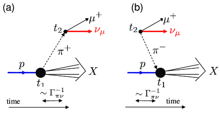
Figure 13: Graphical representation of the two-step processes $p\to n+X+\pi_{\rm virt}^{+}$, $\pi_{\rm virt}^{+}\to{\nu}+\mu^{+}$, as they occur in the neutrino experiment of the OPERA group [41].

iii) Since integration over $z$ in Eq. (5.369) in intermediate reaction states includes all times $-\infty<t_{z}<\infty$, for $t_{y}<t_{z}<t_{x}$, the process occurred at $t_{z}$ is delayed compared to that occurred at $t_{y}$, and for $t_{z}<t_{y}<t_{x}$ the process occurred at $t_{z}$ is advanced compared to that occurred at $t_{y}$. Both time processes should be incorporated as dictated by the Lorentz invariance. In Fig. 13 we demonstrate example of a time delay (a) and an advancement (b) in the specific two-step processes $p\to n+X+\pi_{\rm virt}^{+}$, $\pi_{\rm virt}^{+}\to{\nu}+\mu^{+}$. Such processes play important role in the recent neutrino OPERA experiment [41]. Let the life time of the off-mass-shell pion produced in the process $p\rightarrow n+X+\pi_{\rm virt}^{+}$ is $t_{N\pi}^{\rm dec}=1/\Gamma_{N\pi}$ and in the process $\pi_{\rm virt}^{+}\to{\nu}+\mu^{+}$ it is $t_{\pi\nu}^{\rm dec}=1/\Gamma_{\pi\nu}$. The time $t_{\nu}^{\rm dec}=t_{N\pi}^{\rm dec}+t_{\pi\nu}^{\rm dec}$ characterizes duration of the full two-step process. This means that virtual pions, being produced in the process $p\to n+X+\pi_{\rm virt}^{+}$, undergo in the subsequent process $\pi_{\rm virt}^{+}\to{\nu}+\mu^{+}$ time delays and advances on a time scale $-t_{\pi\nu}^{\rm dec}\lesssim t_{2}-t_{1}\lesssim t_{\pi\nu}^{\rm dec}$, where $t_{2}$ characterizes act of the production of $\nu$ and $t_{1}$, of the absorption of $p$. Note that $t_{N\pi}^{\rm dec}\ll t_{\pi\nu}^{\rm dec}$.

The uncertainty in the production time reflects also the fact that a system undergoing some transition to a new state (decay) does not have a defined energy and is described in quantum mechanics be a wave packet possessing a finite spread in space and time of the order of $1/\Gamma$, cf Eq. (3.228).

iv) One may introduce another time scales similarly to that we introduced in classical and quantum mechanical descriptions. For example, for $1+1$ dimensional problem the quantity

$$t_{\rm soj}^{({\rm 1D})}(a,b;\tau)=\int_{0}^{\tau}{\rm d}t\int_{a}^{b}{\rm d}zF^{({\rm 1D})}(t,z;t,z)/\int{\rm d}zF^{({\rm 1D})}(t,z;t,z)$$ (5.383)

is similar to that given by Eq. (2.3) and (3.180), and for $3+1$ theory,

$$t_{\rm soj}(\Omega,\tau)=\int_{0}^{\tau}{\rm d}t\int{\rm d}^{3}rF(t,\vec{r};t,\vec{r})/\int{\rm d}^{3}rF(t,\vec{r};t,\vec{r})$$ (5.384)

is similar to that given by Eqs. (2.15) and (4.326).

6 Time shifts in quantum kinetics

6.1 Wigner transformation and gradient expansion

Consider slightly inhomogeneous and slowly evolving systems. Then in the spirit of semiclassical approximation degrees of freedom can be subdivided into rapid and short-ranged and slow and long-ranged. For any two-point function $\mathcal{F}(x,y)$, one may introduce the variable $\xi=(t_{1}-t_{2},\vec{r}_{1}-\vec{r}_{2})$, which relates to rapid and short-ranged microscopic processes, and the variable $X=\frac{1}{2}(t_{1}+t_{2},\vec{r}_{1}+\vec{r}_{2})$, which refers to slow and long-ranged collective motions. The Wigner transformation [111], i.e., the Fourier transformation in $\xi=x-y$ to 4-momentum $p$, leads to $\mathcal{F}(X,p)$ functions. Since the Wigner transformation is defined for physical time-space coordinates rather than for contour coordinates one has to decompose the contour integrations into the time-ordered $\{-\}$ and the anti-time ordered $\{+\}$ branches. Two-point functions then become matrices of the contour decomposed $\{-+\}$ components with physical space-time arguments. Thus

$$\mathcal{F}^{ij}(X,p)=\int{\rm d}\xi e^{ip\xi}\,\mathcal{F}^{ij}\left(X+\frac{\xi}{2},X-\frac{\xi}{2}\right),\quad i,j\in\{-+\}$$ (6.385)

leads to a four-phase-space representation of two-point functions.

The Wigner transformation of the Dyson equation (5.369) is straightforward. Taking the difference and half-sum of the Dyson equation (5.369) and the corresponding adjoint equation after the Wigner transformation we arrive at equations

$$iv_{\mu}\partial^{\mu}_{X}G^{ij}(X,p) = \int{\rm d}\xi e^{ip\xi}\int_{C}{\rm d}z\left(\Sigma(x^{i},z)G(z,y^{j})-G(x^{i},z)\Sigma(z,y^{j})\right),$$ (6.386)

$$\widehat{Q}_{X}G^{ij}(X,p) = \sigma^{ij}+\frac{1}{2}\int{\rm d}\xi e^{ip\xi}\int_{C}{\rm d}z\left(\Sigma(x^{i},z)G(z,y^{j})+G(x^{i},z)\Sigma(z,y^{j})\right),$$ (6.387)

where $\sigma^{ij}$ accounts for the integration sense on the two contour branches, cf. Eq. (5.356). For non-relativistic kinematics $v^{\mu}=(1,\vec{p}/m)$, and $\widehat{Q}_{X}=p_{0}-{\vec{p}}^{\,2}/2m-\partial_{\vec{X}}^{2}/8m$. In this matrix notation, two of Eqs. (6.386) and (6.387), involving $G^{-+}$ and $G^{+-}$ on the left-hand side, are known as Kadanoff-Baym equations in the Wigner representation [24]. Particular combinations of these equations lead to the retarded and advanced equations, which completely decouple and involve only integrations over physical times rather than contour times.

We will solely deal with the gradient approximation for slow collective motions by performing the gradient expansion of Eqs. (6.386) and (6.387). This step preserves all the invariances of the $\Phi$ functional in a $\Phi$-derivable approximation [35]. Within the gradient expansion the Wigner transformation of a convolution of two two-point functions entering the Dyson equations (6.387), (6.386) is given by

$$\int{\rm d}\xi e^{ip\xi}\left(\int{\rm d}zf(x,z)\varphi(z,y)\right)\approx f(X,p)\varphi(X,p)+\frac{i\hbar}{2}\{f(X,p),\varphi(X,p)\},$$ (6.388)

where

$$\{f(X,p),\varphi(X,p)\}=\frac{\partial f}{\partial p^{\mu}}\frac{\partial\varphi}{\partial X_{\mu}}-\frac{\partial f}{\partial X^{\mu}}\frac{\partial\varphi}{\partial p_{\mu}}$$ (6.389)

is the Poisson bracket in covariant notation. Note that the smallness of the $\hbar\partial_{X}\cdot\partial_{p}$ comes solely from the smallness of space–time gradients $\partial_{X}$, while momentum derivatives $\partial_{p}$ are not assumed to be small. Such a description is meaningful only if the typical time and space scales are large compared to microscopic ones $|t_{i}-t_{j}|\sim t_{\rm mic}\sim(1/E_{\rm F},1/E_{\rm T})$, $|\vec{r}_{i}-\vec{r}_{j}|\sim r_{\rm mic}\sim(1/p_{\rm F},1/p_{\rm T})$ (for the low energy excitations in the Fermi system and for the Boltzmann gas, respectively, where index $\rm F$ labels the Fermi quantity and $\rm T$, the thermal one).

6.2 Three forms of quantum kinetic equation

Only two real functions of all $G^{ij}(X,p)$ are required for a complete description of the system’s evolution [35]. As these real functions, it is convenient to use the Wigner density $F(X,p)=(\mp)iG^{-+}(X,p)$ and the spectral function $A(X,p)$. The kinetic equation for off-shell particles is ordinary presented in the two different forms: in the Kadanoff-Baym (KB) form, i.e. as it follows right after the first order gradient expansion in the Dyson equation for the Wigner density [24],

$$\widehat{D}\,F(X,p)-\big{\{}\Gamma_{\rm in}(X,p),\Re G^{R}(X,p)\big{\}} = C(X,p),$$ (6.390)

and in the Bottermans-Malfliet (BM) form [32], see discussion of these aspects in [35]. Similarly kinetic equation can be written for $\widetilde{F}(X,p)\equiv iG^{+-}(X,p)$. The collision term

$$C(X,p)=\Gamma^{\rm in}(X,p)\,\widetilde{F}(X,p)-\Gamma^{\rm out}(X,p)\,F(X,p)$$ (6.391)

is the difference of the gain and loss terms, $\Gamma^{\rm in}(X,p)=\mp i\Sigma^{-+}(X,p)$ (in the co-variant notations of [35]) is the reduced production (gain) source term, $\Gamma^{\rm out}(X,p)=i\Sigma^{+-}(X,p)$ is the reduced absorption (loss) term. The differential drift operator is defined as

$$\widehat{D}(\dots)=\big{\{}\Re[G^{-1}(X,p)],\dots\big{\}}=Z^{-1}_{\mu}(X,p)\frac{\partial}{\partial X_{\mu}}+\frac{\partial\Re\Sigma^{R}(X,p)}{\partial X^{\mu}}\frac{\partial}{\partial p_{\mu}},$$ (6.392)

with

$$Z^{-1}_{\mu}(X,p)=\frac{\partial}{\partial p^{\mu}}\Re[G^{-1}(X,p)]=v_{\mu}-\frac{\partial\Re\Sigma^{R}(X,p)}{\partial p^{\mu}},\quad v^{\mu}=\frac{\partial}{\partial p_{\mu}}G_{0}^{-1}(p).$$ (6.393)

Here $G^{-1}_{0}(p)$ is the Fourier transform of the inverse free Green’s function (5.352):

$$G^{-1}_{0}=\left\{\begin{array}[]{ll}p^{2}-m^{2}&\mbox{for relativistic bosons,}\\ p_{0}-{\vec{p}}^{\,\,2}/(2m)&\mbox{for non-rel. particles,}\end{array}\right.$$ (6.396)

$m$ is the mass of the free particle. The BM form is obtained from the KB equation, if one puts $\Gamma^{\rm in}(X,p)=\Gamma(X,p)F(X,p)/A(X,p)$ in the Poisson bracket term. This replacement is legitimate, if one assumes only small (the first gradient order) deviations from the local or global equilibrium (in the local and global equilibrium the collision term $C(X,p)=0$). Then the BM form differs from the KB form only in the second order of the gradient expansion (more precisely in the first order gradient times first order deviation from equilibrium), see [35] for the details. At first glance these equations are equivalent in their common region of validity. However the KB equation has still one important advantage. It fulfills the conservation laws of the Noether 4-current and of the Noether energy-momentum exactly [36, 37] provided self-consistent, i.e., $\Phi$ derivable approximations are used, whereas the BM form fulfills the conservation laws only approximately (up to zero gradients). Moreover the KB equation can be applied not only to description of the relaxation of the system towards the local equilibrium but in many other problems, in which the BM form is not applicable.

The third, non-local, form of the kinetic equation was introduced in [40]:

$$\widehat{D}F(X,p)-\Big{\{}\Gamma(X,p)\frac{F(X,p)}{A(X,p)},\Re G^{R}(X,p)\Big{\}}=C^{\rm NL}(X,p)$$

$$\qquad\qquad\qquad=\Big{(}1+\Big{\{}\frac{1}{A(X,p)},\Re G^{R}(X,p)\Big{\}}\Big{)}\,C^{\rm shift}(X,p)\,,$$ (6.397)

$$C^{\rm shift}(X,p)={C\left(X^{\mu}-\delta X^{\mu},p^{\mu}-\delta p^{\mu}\right)},\quad$$

$$\delta X^{\mu}=\frac{1}{A(X,p)}\frac{\partial\Re G^{R}(X,p)}{\partial{p_{\mu}}},\quad\delta p^{\mu}=-\frac{1}{A(X,p)}\frac{\partial\Re G^{R}(X,p)}{\partial{X_{\mu}}}\,.$$

If we replace $C^{\rm NL}(X,p)\to C(X,p)$ we obtain the BM form. If we expand $C^{\rm NL}(X,p)$ up to first gradient terms we arrive at the KB equation. Thus Eq. (6.397) coincides with the BM form up to the first order gradients and with the KB equation up to second order gradients.

The retarded Green’s function is

$$G^{R}(X,p)=\frac{1}{M(X,p)+i\Gamma(X,p)/2}+O(\partial_{X}^{2})$$ (6.398)

and

$$A(X,p) \equiv -2\Im G^{R}(X,p)\simeq\frac{\Gamma(X,p)}{M^{2}(X,p)+{\textstyle\frac{1}{4}}\Gamma^{2}(X,p)}\,$$ (6.399)

is the spectral function with the “mass” function and the width given by

$$M(X,p)=G^{-1}_{0}(p)-\Re\Sigma^{R}(X,p),\quad\Gamma(X,p)\equiv-2\Im\Sigma^{R}(X,p)=\Gamma^{\rm out}(X,p)\pm\Gamma^{\rm in}(X,p)\,,$$ (6.400)

cf. the introduced above definitions (5.377) and (5.378). We see that expression (6.399) has the same resonance form, as Eqs. (2.67), (2.68) in mechanical example considered in Sect. 2, as Eq. (2.96) in classic-electrodynamical example, and as Eq. (3.302) in quantum mechanical example considered in Sect. 3. Although the solution (6.398), (6.399) is simply algebraic, it is valid up to first-order gradients.

To simplify the further consideration we imply that in relativistic case separation of particle and antiparticle degrees of freedom is performed. Therefore, below we deal with particle species. Antiparticle quantities can be introduced similarly.

In Eq. (6.397) the Wigner densities can be presented as

$$F(X,p)=A(X,p)f(X,p),\quad\widetilde{F}(X,p)=A(X,p)(1\mp f(X,p)),$$ (6.401)

where $f(X,p)$ is a new generalized distribution function. In a local equilibrium this function takes the form

$$f_{\rm l.eq}(X,p)=\frac{1}{e^{[p_{\mu}\,u^{\mu}(X)-\mu(X)]/T(X)}\pm 1},$$ (6.402)

where $u^{\mu}(X)=(1,\vec{u}(X))/\sqrt{1-\vec{u\,}^{2}(X)}$ and $\vec{u}(X)$ is the local velocity of a tiny element of the system. This distribution turns the collision term to zero.

Using Eq. (6.401) we are able to derive other form of the non-local kinetic equation (6.397):

$$\frac{1}{2}A^{2}(X,p)\Gamma(X,p)\Big{(}\widehat{D}f(X,p)-\frac{M(X,p)}{\Gamma(X,p)}\big{\{}\Gamma(X,p),f(X,p)\big{\}}\Big{)}=A(X,p)\,\mathcal{C}^{\rm shift}(X,p),$$

$$\quad\mathcal{C}^{\rm shift}(X,p)=\frac{C^{\rm shift}(X,p)}{A^{\rm shift}(X,p)}\,,\quad A^{\rm shift}(X,p)=A(X^{\mu}-\delta X^{\mu},p^{\mu}-\delta p^{\mu}).$$ (6.403)

Equation (6.2) up to the second-order gradients coincides with the KB equation and up to the first-order gradients coincides with the BM form, cf. the kinetic equation in the BM form, Eq. (3.28) in [35]. Note that besides non-locality introduced by the shift of variables, $C^{\rm shift}$ and $C$ may still include the memory effects, if the generating 2PI $\Phi$ functional contains diagrams with more than two vertices.

The key point which we want further to focus on is the variable shift in the collision term

$$\delta X^{\mu}(X,p) \equiv (\delta t_{f}^{\rm kin},\delta\vec{r}_{f})=\frac{1}{A(X,p)}\frac{\partial\Re G^{R}(X,p)}{\partial{p_{\mu}}}=\frac{1}{2}B^{\mu}(X,p)-\frac{Z^{-1,\mu}(X,p)}{\Gamma(X,p)},$$

$$\delta p^{\mu}(X,p) = -\frac{1}{A(X,p)}\frac{\partial\Re G^{R}(X,p)}{\partial{X_{\mu}}},$$ (6.404)

where

$$B^{\mu}(X,p) =\big{(}B_{0}(X,p),B_{0}(X,p)\,\vec{v}_{\rm gr}(X,p)\big{)}=-2\Im\left[\left(v^{\mu}-\frac{\partial\Re\Sigma^{R}(X,p)}{\partial p_{\mu}}\right)\,G^{R}(X,p)\right]$$ (6.405)

$$=A(X,p)\left[v^{\mu}-\frac{\partial\Re\Sigma^{R}(X,p)}{\partial p_{\mu}}-\frac{M(X,p)}{\Gamma(X,p)}\frac{\partial\Gamma(X,p)}{\partial p_{\mu}}\right]$$

is a flow spectral function and

$$\vec{v}_{\rm gr}(X,p)=\frac{\vec{v}+\frac{\partial\Re\Sigma^{R}(X,p)}{\partial\vec{p}}+\frac{M(X,p)}{\Gamma(X,p)}\frac{\partial\Gamma(X,p)}{\partial\vec{p}}}{v^{0}-\frac{\partial\Re\Sigma^{R}(X,p)}{\partial p_{0}}-\frac{M(X,p)}{\Gamma(X,p)}\frac{\partial\Gamma(X,p)}{\partial p_{0}}}$$ (6.406)

has the meaning of a generalized group velocity of off-mass-shell particles, see Ref. [112]. The latter quantity generalizes expression for the energy $p_{0}$-integrated transport velocity introduced in Ref. [113] and applied for localization phenomena and resonance scattering.

The non-local kinetic equation (6.2) can be rewritten in a more convenient form

$$A_{S}^{\mu}(X,p)\frac{\partial f(X,p)}{\partial{X^{\mu}}}+A(X,p)\Big{[}\frac{\partial\Re\Sigma^{R}(X,p)}{\partial{X_{\mu}}}-\frac{\Gamma(X,p)}{A(X,p)}\frac{\partial\Re G^{R}(X,p)}{\partial{X_{\mu}}}\Big{]}\frac{\partial f(X,p)}{\partial{p^{\mu}}}=A(X,p)\mathcal{C}^{\rm shift}(X,p).$$

(6.407)

This will be the key equation for our further study. Here

$$A^{\mu}_{S}(X,p)={\textstyle\frac{1}{2}}A(X,p)\,\Gamma(X,p)\,B^{\mu}(X,p).$$ (6.408)

The first term on the left-hand side of Eq. (6.407) is the entropy drift term, the second term relates to the spatial changes of a mean field. Dropping in Eq. (6.407) 4-phase space delays/advances in the collision term, i.e. replacing $\mathcal{C}^{\rm shift}(X,p)\to\mathcal{C}(X,p)=C(X,p)/A(X,p)$, we arrive at the BM form of the kinetic equation. In the latter case $A^{\mu}_{S}(X,p)$ is the BM Markovian (BMM) entropy flow spectral function (memory effects are ignored) relating to the entropy flow associated with the BM form of the kinetic equation [35]:

$$S^{\mu}_{\rm{BMM}}(X)={\rm Tr}\int\frac{{\rm d}^{4}p}{(2\pi)^{4}}A^{\mu}_{S}(X,p)\sigma(X,p),\,\,\,$$ (6.409)

where

$$\sigma(X,p)=\mp\big{(}1\mp f(X,p)\big{)}\ln\big{(}1\mp f(X,p)\big{)}-f(X,p)\ln f(X,p),$$ (6.410)

satisfying the equation of motion

$$\frac{\partial}{\partial{X^{\mu}}}S^{\mu}_{\rm{BMM}}(X)=-H(X)={\rm Tr}\int\frac{{\rm d}^{4}p}{(2\pi)^{4}}\ln\frac{1\mp f(X,p)}{f(X,p)}\,C(X,p).$$ (6.411)

Symbol ${\rm Tr}$ implies summation over internal degrees of freedom like spin, etc.

It is easy to demonstrate that the kinetic equation in the BM form conserves the BM effective current exactly [39, 37]

$$j_{S}^{\mu}(X)=e{\rm Tr}\int\frac{{\rm d}^{4}p}{(2\pi)^{4}}A^{\mu}_{S}(X,p)\,f(X,p)\,,$$ (6.412)

provided we work within the $\Phi$-derivable approximation scheme, whereas the Noether current

$$j_{\rm Noether}^{\mu}(X)=e{\rm Tr}\int\frac{{\rm d}^{4}p}{(2\pi)^{4}}v^{\mu}A(X,p)\,f(X,p)$$ (6.413)

and the effective $B$-current

$$j_{B}^{\mu}(X)=e{\rm Tr}\int\frac{d^{4}p}{(2\pi)^{4}}B^{\mu}(X,p)f(X,p)$$ (6.414)

are conserved approximately (up to zero gradient order). Here $e$ is the (electric, baryon, or other) charge of the species and summation over the species, if necessary, is implied.

The maxima in the flow $A_{S}^{\mu}(X,p)$, the flow $B^{\mu}(X,p)$ and $v^{\mu}A(X,p)$ are shifted relatively to each other in the energy-momentum space. Difference of (6.412) and (6.414) with the Noether current (6.413) is that the former two quantities contain contributions of the drag and back flows. The drag flow is associated with the term $-\frac{\partial\Re\Sigma^{R}}{\partial p_{\mu}}A$ and the back flow, with $-\frac{M}{\Gamma}\frac{\partial\Gamma}{\partial p_{\mu}}A$ in the $B^{\mu}$ spectral function (6.405). Presence of these terms causes some additional delays and advances in the propagation of dressed off-shell particles.

The expressions for currents (6.412), (6.413), and (6.414) are derived for the simple form of the 2PI-generating $\Phi$ functional. As soon as the $\Phi$ functional includes diagrams with more than two vertices, there appears additional term in the currents — a so-called ”memory” current $j^{\mu}_{\rm mem}$, see Eq. (6.428) below, and, if the interaction contains derivative couplings, there is yet another ”derivative” current term $j^{\mu}_{\rm der}$. The same relates also to the entropy flow.

If we expand ${\cal C}^{\rm shift}$ in (6.2) up to the first gradients as

$$A(X,p)\,\mathcal{C}^{\rm shift}(X,p) = A(X,p)\left(\Gamma^{\rm in}_{\rm shift}(X,p)-\Gamma_{\rm shift}(X,p)f^{\rm shift}(X,p)\right)$$ (6.415)

$$\simeq C(X,p)+\big{\{}\Gamma^{\rm in}(X,p)-\Gamma(X,p)\,f(X,p),\Re G^{R}(X,p)\big{\}}\,,$$

we arrive at the generalized kinetic equation in the KB form for the distribution function $f(X,p)$:

$$A(X,p)\widehat{D}f(X,p)+f(X,p)\big{\{}\Gamma(X,p),\Re G(X,p)\big{\}}-\big{\{}\Gamma^{\rm in}(X,p),\Re G(X,p)\}=C(X,p),$$ (6.416)

where the collision term

$$C(X,p)=A(X,p)\,\Gamma^{\rm in}(X,p)-A(X,p)\,\Gamma(X,p)\,f(X,p)\,,$$ (6.417)

$$A(X,p)\widehat{D}=\widetilde{B}^{\mu}(X,p)\frac{\partial}{\partial X_{\mu}}+A(X,p)\frac{\partial\Re\Sigma^{R}(X,p)}{\partial X^{\mu}}\frac{\partial}{\partial p_{\mu}},$$

$$\widetilde{B}^{\mu}(X,p)=\Big{(}A(X,p)Z_{0}^{-1}(X,p),A(X,p)\,Z_{0}^{-1}(X,p)\vec{\widetilde{v}}_{\rm gr}(X,p)\Big{)},$$ (6.418)

and the generalized group velocity

$${\widetilde{v}}_{\rm gr}^{i}(X,p)=\frac{Z^{-1,i}(X,p)}{Z_{0}^{-1}(X,p)}=\frac{{v}^{i}+\frac{\partial\Re\Sigma^{R}(X,p)}{\partial{p}^{i}}}{v^{0}-\frac{\partial\Re\Sigma^{R}(X,p)}{\partial p_{0}}},\quad i=1,2,3,$$ (6.419)

differ from the quantities introduced with the help of Eqs. (6.405), (6.406). Recall that $v_{0}=1$ for non-relativistic particles and $2p_{0}$ for relativistic bosons. The BM form is obtained after replacement $\Gamma^{\rm in}(X,p)=\Gamma(X,p)f(X,p)+O(\partial_{x})$ in the second Poisson bracket in (6.416). The KB equation (6.416) exactly conserves the Noether current (6.413), provided approximations are $\Phi$ derivable [36, 37], and it approximately (up to zero-gradient order) conserves the effective current (6.412) and the effective current (6.414).

Note that, since for off-mass-shell particles $p_{0}$ and $\vec{p}$ can vary independently, the value $\widetilde{v}_{\rm gr}(X,p)$ is not necessarily limited from the above by the velocity of light, it might be even not positive definite. Also, the factor $Z_{0}^{-1}(X,p)$ is not, in general, positive definite that leads to a non-trivial procedure of the particle-antiparticle separation for virtual particles. As known [114], in the quasiparticle limit $Z^{\rm qp}_{0}(X,p_{0}(\vec{p}),\vec{p})>0$ determines the quasiparticle spectrum branches and the branches with $Z^{\rm qp}_{0}<0$ are related to the anti-quasiparticles after the replacement $p_{0}\to-p_{0}$ and $\vec{p}\to-\vec{p}$. To be specific, we will further assume $Z_{0}^{-1}>0$, considering only the particle and not anti-particles.

The spectral functions $A$, $B_{0}$, $A_{S}^{0}$ fulfill sum-rules

$$\int B_{0}(X,p)\frac{{\rm d}p_{0}}{2\pi}=\int v^{0}A(X,p)\frac{{\rm d}p_{0}}{2\pi}=\int A_{S}^{0}(X,p)\frac{{\rm d}p_{0}}{2\pi}=1\,,$$ (6.420)

cf. the sum-rules (2.34), (2.69) and (3.279), (3.291), which we obtained in classical and quantum mechanics. Note that the sum-rule for $A(x,p)$ follows directly from the canonical equal-time (anti) commutator relations for (fermionic) bosonic field operators.

Having at hand the kinetic equation for $F(X,p)$ (either in KB or in BM form) and the algebraic equation for $A$ is sufficient to recover all kinetic quantities. However there exists still one more, so called the mass-shell equation [35], which, as well as the KB equation (6.416), follows from the full Dyson equations expanded up to the first gradient order:

$$M(X,p)\,A(X,p)\,f(X,p)-\Re G^{R}(X,p)\Gamma^{\rm in}(X,p) =\frac{1}{4}\big{\{}\Gamma(X,p),f(X,p)A(X,p)\big{\}}$$ (6.421)

$$-\frac{1}{4}\big{\{}\Gamma^{\rm in}(X,p),A(X,p)\big{\}}.$$

Presenting $\Gamma^{\rm in}(X,p)=f(X,p)\,\Gamma(X,p)+\delta\Gamma^{\rm in}(X,p)$, $\Gamma^{\rm out}(X,p)=\big{(}1\mp f(X,p)\big{)}\Gamma(X,p)+\delta\Gamma^{\rm out}(X,p)$, such that in equilibrium $\delta\Gamma^{\rm in}_{\rm eq}(X,p)=\delta\Gamma^{\rm out}_{\rm eq}(X,p)=0$, and using Eq. (6.400), from (6.421) we find

$$\delta\Gamma^{\rm in}(X,p)=\frac{1}{4\Re G^{R}(X,p)}\big{\{}f(X,p),A(X,p)\,\Gamma(X,p)\big{\}}+O(\partial_{x}^{2})=\mp\delta\Gamma^{\rm out}(X,p).$$ (6.422)

Generally speaking the mass-shell equation should be considered on equal footing with the kinetic equation. Ref. [35] proved equivalence of this equation to the kinetic equation in the BM form up to first gradients. However in general case equivalence of (6.421) and the KB equation (6.416) is not proven.

6.3 Memory effects

A general treatment of the memory effects is a cumbersome task. Following Ref. [35], as an example, consider a system of non-relativistic fermions interacting via contact two-body potential $V_{0}$. The self-energy up to three-vertex diagram becomes

$$-i\Sigma = -i\left(\Sigma^{(1)}+\Sigma^{(2)}+\Sigma^{(3)}\right)=\includegraphics[width=199.16928pt]{Kin-mem-S.eps}\,\,.$$ (6.423)

The local part of the collision term is presented in the form

$$C^{(2)}+C_{\rm loc}^{(3)} = d^{2}\int\frac{{\rm d}^{4}p_{1}}{(2\pi)^{4}}\frac{{\rm d}^{4}p_{2}}{(2\pi)^{4}}\frac{{\rm d}^{4}p_{3}}{(2\pi)^{4}}\left(\left|\parbox{19.91692pt}{\includegraphics[width=19.91692pt]{Kin-mem-vert.eps}}+\parbox{22.76219pt}{\includegraphics[width=22.76219pt]{Kin-mem-C-loop.eps}}\right|^{2}-\left|\parbox{22.76219pt}{\includegraphics[width=22.76219pt]{Kin-mem-C-loop.eps}}\right|^{2}\right)$$ (6.424)

$$\times(2\pi)^{4}\delta^{4}\left(p+p_{1}-p_{2}-p_{3}\right)\left(F_{2}\,F_{3}\,\widetilde{F}\,\widetilde{F}_{1}-\widetilde{F}_{2}\,\widetilde{F}_{3}\,F\,F_{1}\right),$$

where all the vertices in the off-shell scattering amplitudes are of the same sign, say $"-"$ for definiteness, i.e. there are no $"+-"$ and $"-+"$ Green’s functions left, $d$ accounts summation over internal degrees of freedom, e.g. spin. Now the collision term contains a nonlocal part due to the last diagram (6.423).

The current and the entropy flows are expressed in terms of the loop functions

$$L^{jk}(x,y)=\parbox{56.9055pt}{\includegraphics[width=56.9055pt]{Kin-mem-loop.eps}}$$

which in the Wigner representation takes the form

$$L^{jk}(X,p)=\int\frac{{\rm d}^{4}p}{(2\,\pi)^{4}}\widetilde{L}^{jk}(X,p^{\prime}+p,p^{\prime})\,,$$ (6.425)

where

$$\widetilde{L}^{jk}(X,p^{\prime}+p,p^{\prime})=d\,iV_{0}\,iG^{jk}(X,p^{\prime}+p)\,iG^{kj}(X,p^{\prime})\,.$$ (6.426)

The first-order-gradient memory correction to the collision term induced by the third graph (6.423) is

$$C_{\rm mem}^{(3)}(X,p)=\left[\Sigma_{+-,{\rm mem}}^{(3)}(X,p)\,G^{-+}(X,p)-G^{+-}(X,p)\,\Sigma_{-+}^{(3),{\rm mem}}(X,p)\right]$$

$$=\frac{i}{2}\int\frac{{\rm d}^{4}p^{\prime}}{(2\pi)^{4}}\frac{1}{d}\left[\widetilde{L}^{+-}(X,p^{\prime}+p,p)-\widetilde{L}^{-+}(X,p^{\prime}+p,p)\right]\big{\{}L^{+-}(X,p^{\prime}),L^{-+}(X,p^{\prime})\big{\}}_{p^{\prime},X}\,.$$ (6.427)

The memory current follows from integration of (6.3):

$$j^{\mu}_{\rm mem}(X)=e\,\int\frac{{\rm d}^{4}p}{(2\pi)^{4}}\frac{i}{2}L^{+-}(X,p)L^{-+}(X,p)\frac{\partial}{\partial p_{\mu}}\big{(}L^{+-}(X,p)+L^{-+}(X,p)\big{)}\,.$$ (6.428)

Expression for the entropy flow is more cumbersome but it simplifies in case of the local equilibrium:

$$[S^{\mu}_{\rm mem}(X)]_{\rm l.eq}=\int\frac{{\rm d}^{4}p}{(2\pi)^{4}}\frac{i}{2}L^{-+}(X,p)\,L^{+-}(X,p)\left[\ln\frac{L^{+-}(X,p)}{L^{-+}(X,p)}-1\right]\frac{\partial L^{-+}(X,p)}{\partial p_{\mu}}.$$ (6.429)

6.4 Time advances and delays

It is rather natural to expect that the time and the position characterizing collisions of propagating particles undergo some shifts, if one incorporates that collisions are not instant. In accordance with the uncertainty principle and the ergodicity the energy and the momentum are shifted as well. This is taken into account in the non-local form of the kinetic equation (6.397), (6.2), see also Eq. (6.404). These effects are absent in the kinetic equation written the BM form. In Ref. [35] the corresponding Poisson bracket terms in the KB kinetic equation (see Eq. (6.416)) responsible for this phenomenon were associated with quantum fluctuations.

From (6.404) we find for the time delay/advance of collisions:

$$\delta t_{\rm f}^{\rm kin}=\delta t_{\rm s}^{B}-t_{\rm col}\,,\quad\delta t_{\rm s}^{B}=B_{0}/2\,,\quad t_{\rm col}=Z_{0}^{-1}/\Gamma\,.$$ (6.430)

Here and further on in this subsection we will not write out the arguments $(X,p)$ of the quantities, unless it is explicitly needed. The value $\delta t_{\rm s}^{B}$ can be formally expressed through the quantity having the meaning of an in-medium scattering phase shift [40]

$$\delta t_{\rm s}^{B}=\frac{B_{0}}{2}\equiv\frac{\partial\delta(n)}{\partial p_{0}},\quad\tan\delta(n)\equiv-\frac{\Gamma}{2M},$$ (6.431)

where $n=j^{0}_{\rm Noether}$ indicates dependence of $\delta$ on the particle density. Note that the quantity (6.431) describes the delay/adwancement of the dressed particles (or the corresponding group of waves) at arbitrary distances in difference with a similar quantity $\delta t_{\rm s}$ (4.335), which we exploited in description of the resonance quantum mechanical scattering, showing delay/advance of the scattered waves, as measured at large distances. The second relation (6.431) demonstrates measure of proximity of the virtual particle to the mass shell. In the virial limit, $\frac{B_{0}}{2}\to\frac{\partial\delta}{\partial p_{0}}$, where $\delta$ has already the meaning of the real scattering phase shift. E.g. for the $\pi N\Delta$ system, the $B_{0}^{\Delta}$ spectral function of the $\Delta(1232)$ isobar relates to the energy variation of the scattering phase shift $\delta_{33}^{\pi N}$ of the $P_{33}$ partial wave coupled to the $\Delta$ resonance. For the pion, $B_{0}^{\pi}$ in the virial limit relates to the the phase shift of the nucleon hole – $\Delta$ scattering. For the nucleon, $B_{0}^{N}$ relates to $\delta_{\pi\Delta}$. Since following Eq. (6.405) $B_{0}$ is expressed through $A$, the scattering time $\delta t_{\rm s}^{B}$ can be presented as the sum of the Noether scattering delay and the drag and the back delay/advance terms:

$$\delta t_{\rm s}^{B}=\delta t_{\rm s}^{A}+\delta t_{\rm s}^{\rm drag}+\delta t_{\rm s}^{\rm back},$$

$$\delta t_{\rm s}^{A}=\frac{v_{0}A}{2}>0,\quad\delta t_{\rm s}^{\rm drag}=-\frac{A}{2}\frac{\partial\Re\Sigma^{R}}{\partial p_{0}},\quad\delta t_{\rm s}^{\rm back}=-\frac{AM}{2\Gamma}\frac{\partial\Gamma}{\partial p_{0}}.$$ (6.432)

The collision time $t_{\rm col}$ in Eq. (6.430) has the meaning of the average time between collisions. The value $t_{\rm col}$ does not contain factor 2 compared to the classical decay time $t^{\rm cl}_{\rm dec}$ given by Eq. (2.27) of Sect. 2, although in both cases $\Gamma$ enters the poles of the retarded Green’s function similarly. This is because $t_{\rm col}$ describes dynamics of the Green’s function (quadratic form) rather than dynamics of the classical field ($z$-variable in classical mechanics). Also, compared to the quantities: $t^{\rm cl}_{\rm dec}$, see Eq. (2.27) Sect. 2, $t_{\rm dec}$, $t^{\rm scl}_{\rm dec}$, see Eqs. (4.334), (4.339) Sect. 3, the value $t_{\rm col}$ contains additional renormalization factor, cf. also Eq. (5.382) Sect. 5. Thereby the collision time can be presented as the sum of the decay time and the drag delay/advance terms:

$$t_{\rm col}=t_{\rm dec}+\delta t_{\rm col}^{\rm drag},$$ (6.433)

$$t_{\rm dec}=\frac{v_{0}}{\Gamma}>0,\quad\delta t_{\rm col}^{\rm drag}=-\frac{\partial\Re\Sigma^{R}}{\partial p_{0}}\frac{1}{\Gamma}.$$

The value $\delta t_{\rm f}^{\rm kin}$ given by Eq. (6.430) can be as positive as negative. The sum-rules (6.420) for $A$, $B_{0}$ and $A_{S}^{0}$ can be now presented as

$$\int\frac{{\rm d}p_{0}}{2\pi}\delta t_{\rm s}^{A}=\int\frac{{\rm d}p_{0}}{2\pi}\delta t_{\rm s}^{B} =\int\frac{{\rm d}p_{0}}{2\pi}\delta t_{\rm s}^{A_{S}}=\frac{\hbar}{2},\quad\delta t_{\rm s}^{A_{S}}=\frac{A_{S}}{2}\,,$$ (6.434)

$$\int\frac{{\rm d}p_{0}}{2\pi}\big{(}t_{\rm col}+\delta t_{\rm f}^{\rm kin}\big{)}=\frac{\hbar}{2}.$$ (6.435)

Thus, in accord with the energy-time uncertainty principle, cf. [57, 115], $\delta t_{\rm s}^{B}$, $\delta t_{\rm s}^{B}$, $\delta t_{\rm s}^{A_{S}}$ are minimal resolution times of the corresponding wave packets. The collision time $t_{\rm col}\sim t_{\rm dec}$ is the time needed for the decay of unstable system. The value $\delta t_{\rm f}^{\rm kin}$ is the minimal resolution time counted from the collision time, i.e. an average time interval between two successive collisions. The corrected causality condition for collisions should now read as

$$t-r/v_{\rm gr}-\delta t_{\rm f}^{\rm kin}\geq 0.$$ (6.436)

In Sect. 3 we present the relation between the level density and the particle scattering phase shift. The density of states is often determined as [116]:

$$\frac{{\rm d}N^{\rm level}_{A}}{{\rm d}p_{0}/(2\pi)}=\int\frac{{\rm d}^{3}X{\rm d}^{3}p}{(2\pi)^{3}}v^{0}A(X,p_{0},\vec{p}).$$ (6.437)

Thereby in accord with Eq. (6.413) the level density (6.437) is related to the Noether particle density,

$$\frac{{\rm d}N^{\rm Noether}}{{\rm d}^{3}X{\rm d}p_{0}/(2\pi)}=\frac{{\rm d}N^{\rm level}_{A}}{{\rm d}^{3}X{\rm d}p_{0}/(2\pi)}f(X,p_{0},\vec{p}).$$ (6.438)

Note that even in the limit of a small width the spectral density $A$ should include both the quasiparticle term and a regular terms, see Eq. (6.455) below, so that in the case of the conserved number of particles (e.g. baryons) $N^{\rm Noether}$ would coincide with the full number of particles: with the only quasiparticle Green’s function Eq. (6.437) becomes incorrect.

We could introduce the level density of interacting particles differently relating it to the interacting particle density (6.412), cf. Ref. [117],

$$\frac{{\rm d}N^{\rm level}_{A_{S}}}{{\rm d}p_{0}/(2\pi)}=\int\frac{{\rm d}^{3}X{\rm d}^{3}p}{(2\pi)^{3}}A_{S}^{0}(X,p_{0},\vec{p}),$$ (6.439)

or relating it to (6.414) with $B^{0}$ spectral function [118]

$$\frac{{\rm d}N^{\rm level}_{B}}{{\rm d}p_{0}/(2\pi)}=\int\frac{{\rm d}^{3}X{\rm d}^{3}p}{(2\pi)^{3}}B^{0}(X,p_{0},\vec{p})\,.$$ (6.440)

Since following Eq. (4.342) in the virial limit the level density is related to the Wigner delay time, from Eqs. (6.437), (6.439), and (6.440) we find relations

$$\delta t_{\rm W}^{\rm A}=v_{0}A,\quad\delta t_{\rm W}^{A_{S}}=A_{S},\quad\delta t_{\rm W}^{B}=B_{0}.$$ (6.441)

For the non-relativistic particle scattering on a potential $B_{0}=A$ and with $\delta t_{\rm W}^{B}$, as well as with $\delta t_{\rm W}^{A}$, we recover results (4.321), (4.335) derived in Sect. 4. For multi-component systems the total Noether current can be presented as $j^{\rm tot}_{\mu}=\sum j^{\rm Noether}_{\nu}$, see Ref. [34]. On the other hand, the interaction between different species can be redistributed in many ways. For example, the interaction from some species can be redistributed to other ones, cf. Ref. [119]. In the latter case the currents of some properly dressed species are described by Eq. (6.439) or by Eq. (6.440), whereas some other species undergo free motion. For example, for the case of a resonance, like the $\Delta$ or $\rho$-meson resonances in hadron physics, the $B_{0}$-function relates to the energy variations of scattering phase shift of the scattering channel coupling to the resonance in the virial limit [118, 120]. Similarly, in a quantum mechanical scattering divergent and scattered waves are relevant quantities only at large distances, being strongly distorted at short distances near the scatterer.

From Eq. (6.428) using Eqs. (4.342), (6.440), and (6.441) we may also recover the memory Wigner delay/advance time

$$\delta t^{\rm mem}_{\rm W}=\frac{1}{2}\frac{\partial({L}^{+-}+{L}^{-+})}{\partial p_{0}}{L}^{+-}{L}^{-+},$$ (6.442)

provided self-energies include diagrams with more than two vertices. The value $\delta t^{\rm mem}_{\rm W}\propto V_{0}^{3}$ and therefore $\delta t^{\rm mem}_{\rm W}$ disappears in the virial limit.

Finally, note that the quantities $t_{\rm soj}^{({\rm 1D})}(a,b;\tau)$ given by Eq. (5.383) and $t_{\rm soj}(\Omega,\tau)$ given by (5.384), where $F$ is the exact non-equilibrium Green’s function, have the same form, being expressed through the Wigner density $F$ in the Wigner representation.

6.4.1 Time advances and delays for Wigner resonances

For the Wigner resonances $\Re\Sigma^{R}$ and $\Gamma$ are assumed to be independent on $p_{0}$ and Eq. (6.430) is simplified as

$$\delta t_{\rm f}^{\rm kin}=\delta t_{\rm s}^{B}-t_{\rm col}=-\frac{M^{2}-\Gamma^{2}/4}{\Gamma(M^{2}+\Gamma^{2}/4)}=\delta t_{\rm f}=\delta t_{\rm s}^{A}-t_{\rm dec}.$$ (6.443)

The energy weighted time shift $\int\frac{{\rm d}p_{0}}{2\pi}\Gamma A\delta t_{\rm f}^{\rm kin}=0$.

The value $\delta t_{\rm s}^{A}=\frac{\Gamma/2}{M^{2}+\Gamma^{2}/4}>0$ coincides with the scattering time delay, $\delta t_{\rm s}=\frac{\partial\delta}{\partial p_{0}}$, introduced in quantum mechanics, see Eq. (4.318). The collision time coincides with the quantum mechanical time, $\delta t_{\rm vol}=\frac{1}{2\mbox{sin}^{2}\delta}\frac{\partial\delta}{\partial p_{0}}$, when all the delays are put into scattering, see Eq. (4.326), (4.334). Thus, the value $-t_{\rm col}=-t_{\rm dec}=-1/\Gamma<0$ has the meaning of the collision time advance. The value $\delta t_{\rm f}^{\rm kin}$ given by (6.443) coincides with the quantity $\delta t_{\rm f}=-\delta t_{\rm i}=-\frac{\cos(2\delta)}{2\sin^{2}\delta}\frac{\partial\delta}{\partial p_{0}}$, see Eq. (4.333), being a forward delay/advance time. A propagating wave packet gets a delay/advance $\delta t_{\rm i}$ due to interference of the incident and reflected waves. The collision term gets corresponding advance/delay $\delta t_{\rm f}=-\delta t_{\rm i}$, being the scattering time counted from the collision time, since actual collision for the particles with the width may occur a time $\sim t_{\rm col}$ earlier than it happens in the case of the zero width. In the limit $|M|\ll\Gamma$ there is a time delay $\delta t_{\rm f}=1/\Gamma$ and for $|M|\gg\Gamma$ there arises a time advance $\delta t_{\rm f}=-1/\Gamma$, and for $|M|=\Gamma/2$, $\delta t_{\rm f}=0$.

6.5 Test particle method

The conserving feature is especially important for devising numerical simulation codes based on the kinetic equation. If a test-particle method is used, one should be sure that the number of test particles is conserved exactly rather than approximately. In the test-particle method the distribution function $F$ (not $f$) satisfying Eq. (6.397) is represented by an ensemble of test particles [40]

$$F(X,p)\sim\sum_{i}\delta^{(3)}\left({\vec{x}}-{\vec{x}}_{i}(t)\right)\delta^{(4)}\left({p}-{p}_{i}(t)\right),$$ (6.444)

where the $i$-sum runs over test particles, $p=(p^{0},\vec{p}\,)$. Then the drift term in KB equation for $F$ (derived from (6.397) if one expands the collision term in gradients including the first gradient terms) just corresponds to the classical motion of these test particles subjected to forces inferred from $\Re\Sigma^{R}(X,p)$, while the collision term gives stochastic change of test-particle’s momenta, when their trajectories “cross”. For a direct application of this method, however, there is a particular problem with the kinetic equation in the KB form. Appearing additional Poisson-bracket term $\{\Gamma^{\rm in},\Re G^{R}\}$ spoils this simplistic picture, since derivatives acting on the distribution function $F$ arise here only indirectly and thus cannot be included in the collision-less propagation of test particles. This problem, of course, does not prevent a direct solution of the KB kinetic equation applying lattice methods, which are, however, much more complicated and time-consuming as compared to the test particle approach.

The effective BM-current was used in [121] as a basis for the construction of a test-particle ansatz for numerical solution of the nonrelativistic BM kinetic equation. To fulfill the effective current conservation one introduces the test-particle ansatz for

$$\frac{1}{2}\Gamma B_{0}F(X,p)\sim\sum_{i}\delta^{(3)}\left({\vec{x}}-{\vec{x}}_{i}(t)\right)\delta^{(4)}\left(p-p_{i}(t)\right),$$ (6.445)

rather than for the distribution function itself. Note that the energy $p^{0}_{i}(t)\equiv E_{i}(t)$ of the test particle is an independent coordinate, not restricted by a mass-shell condition. Ref. [122] used this test-particle ansatz in the relativistic case.

The BM kinetic equation together with ansatz (6.445) for the distribution function result in the set of equations for evolution of parameters of the test particles between collisions

$$\frac{{\rm d}\vec{x}_{i}}{{\rm d}t} = \frac{1}{v_{0}-\partial_{E_{i}}\Re\Sigma^{R}-(M/\Gamma)\partial_{E_{i}}\Gamma}\left({\vec{v}}_{i}+\nabla_{p_{i}}\Re\Sigma^{R}+(M/\Gamma)\nabla_{p_{i}}\Gamma\right),$$ (6.446)

$$\frac{{\rm d}\vec{p}_{i}}{{\rm d}t} = \frac{1}{v_{0}-\partial_{E_{i}}\Re\Sigma^{R}-(M/\Gamma)\partial_{E_{i}}\Gamma}\left(\nabla_{x_{i}}\Re\Sigma^{R}+(M/\Gamma)\nabla_{x_{i}}\Gamma\right),$$ (6.447)

$${\dot{E}}_{i} = \frac{1}{v_{0}-\partial_{E_{i}}\Re\Sigma^{R}-(M/\Gamma)\partial_{E_{i}}\Gamma}\left(\partial_{t}\Re\Sigma^{R}+(M/\Gamma)\partial_{t}\Gamma\right).$$ (6.448)

All function on the right-hand side are evaluated in the point $(t,\vec{x}_{i}(t),E_{i}(t),\vec{p}_{i}(t))$. These equations of motion, in particular, yield the time evolution of the mass term $M$, of a test particle [122, 121]

$$\frac{{\rm d}M_{i}}{{\rm d}t}=\frac{M_{i}}{\Gamma_{i}}\frac{{\rm d}\Gamma_{i}}{{\rm d}t},$$ (6.449)

the origin of which can be traced back to the additional term $\{\Gamma F/A,\Re G^{R}\}$ in the BM equation. Here $M_{i}(t)=M[t,{\vec{x}}_{i}(t);E_{i}(t),{\vec{p}}_{i}(t)]$ measures an “off-shellness” of the test particle, and $\Gamma_{i}(t)=\Gamma[t,{\vec{x}}_{i}(t);E_{i}(t),{\vec{p}}_{i}(t)]$. Equation of motion (6.449) yields $|M_{i}|=\alpha_{i}\Gamma_{i}$, where $\alpha_{i}>0$ do not depend on time, and implies that once the width drops in time the particles are driven towards the mass on-shell, i.e. to $M=0$. This clarifies the meaning of the additional term $\{\Gamma F/A,\Re G^{R}\}$ in the off-shell BM kinetic equation (which follows from (6.397), if one suppresses variable shifts in the collision term): it provides the time evolution of the off-shellness.

For the non-local form of the kinetic equation [40] the set of equations for evolution of parameters of the test particles between collisions is the same as in the BM case. The only difference with the BM case is that collisions of test particles occur with certain time (and space) delay (or advance) as compared with the instant of their closest approach to each other.

Following Eq. (6.404) the shift of the space variables is

$$\delta\vec{x}=\frac{1}{A}\frac{\partial\Re G^{R}}{\partial\vec{p}}=\delta\vec{x}_{\rm drift}+\delta\vec{x}_{\rm col}=\frac{1}{2}\vec{B}+\vec{\widetilde{v}}_{\rm gr}t_{\rm col}.$$ (6.450)

We can further express the spatial shift in terms of time delays and velocity $\frac{{\rm d}\vec{x}}{{\rm d}t}$ of a test particle on its trajectory, cf. Eq. (6.446),

$$\delta\vec{x}_{i}=\frac{{\rm d}\vec{x}_{i}}{{\rm d}t}\delta t_{i,{\rm s}}^{B}+\vec{\widetilde{v}}_{i,{\rm gr}}t_{i,{\rm col}}.$$ (6.451)

Equation (6.451) demonstrates that before a delayed/advanced collision the test particle moves along its trajectory. Therefore, the scattering time delay $\delta t_{i,{\rm s}}^{B}$ unambiguously results in a definite space shift. The collision itself is associated with an additional time delay $t_{i,{\rm col}}$, which implies that the collision is not instant, as it is treated in the BM kinetic equation, but requires certain time for complete decoupling from intermediate states (e.g., the pion spends some time in the intermediate $\Delta$–nucleon-hole state, a soft photon requires certain time to be formed in multiple collisions of the proton with neutrons). Therefore, this additional delay gives rise to an additional shift of the particle with respect to its “collisionless” trajectory (6.446).

6.6 Quasiparticle limit

The quasiparticle limit is understood, as the limit, when Green’s functions are computed at $\Im\Sigma^{R}\rightarrow 0$. The quasiparticle width $\Gamma_{\rm qp}(X,\vec{p})=-2\Im\Sigma^{R}(X,\vec{p},A\to A_{\rm qp})$ is then calculated with the quasiparticle Green’s functions and the associated quasiparticle spectral functions $A_{\rm qp}$. The letter reduces in this limit ($|M|=\alpha\Gamma$, $|\alpha|\gg 1$) to,

$$A_{\rm qp}(X,p)=2\pi Z_{0}^{\rm qp}(X,\vec{p}\,)\,\delta\left(p_{0}-E_{p}(X,\vec{p}\,)\right),\quad Z_{0}^{\rm qp}(X,\vec{p}\,)=\left(v^{0}-\frac{\partial\Re\Sigma^{R}(X,p)}{\partial p_{0}}\right)_{p_{0}=E_{p}(X,\vec{p}\,)}^{-1}\,,$$ (6.452)

where $E_{p}(X,\vec{p})$ stands for the energy of a quasiparticle, being the root of the dispersion relation

$$M(X,p_{0}=E_{p}(X,\vec{p}\,),\vec{p})=0,$$ (6.453)

$Z_{0}^{\rm qp}(X,\vec{p}\,)>0$ on the quasiparticle branch $p_{0}=E_{p}(X,\vec{p}\,)$.

The quasiparticle spectral function does not fulfill the exact sum rule (6.420) but fulfills the corresponding quasiparticle sum-rule

$$\int Z_{0}^{{\rm qp}}(X,\vec{p}\,)\,A_{\rm qp}(X,p)\frac{{\rm d}p_{0}}{2\pi}=1\,.$$ (6.454)

Formally, within the quasiparticle picture this problem is avoided by a renormalization, after which one may already deal only with the quasiparticle degrees of freedom, being well separated from the degrees of freedom in the continuum. The reason for the difference between the exact and quasiparticle sum-rules is that the quasiparticle current $j_{\rm qp}^{\mu}=(j_{B}^{\rm qp})^{\mu}=(j_{S}^{\rm qp})^{\mu}$ includes the quasiparticle drag flow and, thereby, differs from the Noether current. This difference is compensated due to the conservation of the Noether current by the presence of the back flow, as a back reaction of the whole energy sea to the particle drag flow. Thus, the exact sum-rule (6.420) for $A$ is recovered, provided one includes the width term. It is easily demonstrated in case of a weak interaction [123]. Then

$$A(X,p)\simeq 2\pi Z_{0}^{\rm qp}(X,\vec{p}\,)\delta\big{(}M(X,p)\big{)}+\mathcal{P}\frac{\Gamma(X,p)}{M^{2}(X,p)}\simeq 2\pi\,\delta(p_{0}-E_{p}(X,\vec{p}\,))\,,$$ (6.455)

where $\mathcal{P}$ indicates the principal value. The required sum-rule is recovered after using of the Kramers-Kronig relation between $\Gamma$ and $\Re\Sigma$.

The integration of all three forms of the kinetic equation, the BM form, the KB equation (6.416), and the non-local Eq. (6.407) over ${\rm d}p_{0}/(2\pi)$ yields one and the same kinetic equation describing the quasiparticle propagation in matter:

$$\frac{\partial f_{\rm qp}(X,\vec{p}\,)}{\partial{t}}+\vec{v}^{\,\rm qp}_{\rm gr}(X,\vec{p}\,)\,\nabla f_{\rm qp}(X,\vec{p}\,)-\nabla E_{p}(X,\vec{p}\,)\frac{\partial f_{\rm qp}(X,\vec{p})}{\partial\vec{p}}=C_{\rm qp}(X,\vec{p}\,)\,,$$ (6.456)

here $E_{p}$ obeys mass-shell condition (6.453),

$$C_{\rm qp}^{\rm shift}(X,\vec{p}\,)=\int\frac{{\rm d}p_{0}}{2\pi}A_{\rm qp}(X,p)\,\mathcal{C}^{\rm shift}(X,p;A\to A_{\rm qp})\to C_{\rm qp}(X,\vec{p}\,)$$

and the quasiparticle group velocity is

$$\vec{{v}}^{\,\rm qp}_{\rm gr}(X,\vec{p}\,)=\frac{\partial E_{p}(X,\vec{p}\,)}{\partial\vec{p}}=\frac{\left(\vec{v}+\frac{\partial\Re\Sigma^{R}(X,p)}{\partial\vec{p}}\right)_{p_{0}=E_{p}(X,\vec{p}\,)}}{\left(v^{0}-\frac{\partial\Re\Sigma^{R}_{\rm qp}(X,p)}{\partial p_{0}}\right)_{p_{0}=E_{p}(X,\vec{p}\,)}}.$$ (6.457)

Memory effect corrections to the collision term derived in the extended quasiparticle approximation were considered in Ref. [124].

In the quasiparticle limit the BMM entropy, Eq. (6.409), reads

$$S^{\mu}_{\rm qp}=\int\frac{{\rm d}^{3}p}{(2\pi)^{3}}\sqrt{1-[\vec{v}\,_{\rm gr}^{\rm qp}(X,\vec{p}\,)]^{2}}[u_{\rm gr}^{\rm qp}(X,\vec{p}\,)]^{\mu}\,\sigma_{\rm qp}(X,\vec{p}\,),$$ (6.458)

where we introduced notation

$$[u_{\rm gr}^{\rm qp}(X,\vec{p}\,)]^{\mu}=\left(\frac{1}{\sqrt{1-[\vec{v}\,_{\rm gr}^{\rm qp}(X,\vec{p}\,)]^{2}}},\frac{\vec{v}\,_{\rm gr}^{\rm qp}(X,\vec{p}\,)}{\sqrt{1-[\vec{v}\,_{\rm gr}^{\rm qp}(X,\vec{p}\,)]^{2}}}\right).$$ (6.459)

The quasiparticle group velocity can significantly differ from the phase velocity. In atomic Bose-Einstein condensates [125] the light can be slowed down to the speed 17 m/s (a so-called slow light). The light also becomes ultra-slow in the hot atomic vapor of rubidium [126]. On the other hand, the quasiparticle group velocity can easily exceed the velocity of light in medium $c(n)<c$. It manifests as the Cherenkov radiation. An instability of quasiparticle modes also arises in a moving medium [127, 128, 129] (even if the modes are stable in the static medium), provided $|\vec{u}||\vec{p}|>E_{p}(p)$, where $\vec{u}$ is the speed of the medium and $E_{p}(p)$ is the quasiparticle spectrum branch. As the result, a spatially inhomogeneous condensate of Bose excitations may be formed. This phenomenon is similar to the Cherenkov effect and the shock wave generation.

Obviously, the values of time delays are unlimited. The question about a possible limitation on the time advance and possibility to have $v^{\rm gr}_{\rm qp}>c$ are subtle issues. As argued in Ref. [94, 95], such a possibility does not contradict causality. However the velocity of the wave front $v_{\rm fr}$ should always be limited by $c$, see Ref. [18] and references therein. An apparent superluminal propagation manifested in some laser experiments can be understood as consequence of a reshaping of the pulse envelope by interaction within the medium, see discussion in [14, 15, 18, 16]. Although formally $v_{\rm gr}$ exceeds $c$, the forward wave front moves with velocity $\leq c$, as it should be. There are also arguments that the advance of the pulse of light in materials is generally limited only by few pulse widths (so called fast light). Thereby, the interpretation of a negative group delay as a superluminal propagation is according to Ref. [16] a semantic question, since the speed of the information transport never exceeds $c$, see Ref. [17].

Reference [113] used the $p_{0}$-averaged BM equation and averaged distributions,

$$f^{B}(X,\vec{p}\,)=\int\frac{{\rm d}p_{0}}{2\pi}B_{0}(X,p)f(X,p)\,.$$ (6.460)

Averaged values

$$\vec{v}_{\rm gr}^{\,B}(X,\vec{p}\,)=\int\frac{{\rm d}p_{0}}{2\pi}B_{0}(X,p)\,\vec{v}_{\rm gr}(X,p),\quad\vec{\widetilde{v}}_{\rm gr}^{\,B}(X,\vec{p}\,)=\int\frac{{\rm d}p_{0}}{2\pi}\widetilde{B}_{0}(X,p)\,\vec{\widetilde{v}}_{\rm gr}(X,p)\,,$$

$$\vec{v}_{\rm gr}^{\,S}(X,\vec{p}\,)=\int\frac{{\rm d}p_{0}}{2\pi}A_{S}(X,p)\,\vec{v}_{\rm gr}(X,p)\,,$$ (6.461)

yield one and the same value $\vec{v}^{\,\rm gr}_{\rm qp}$ in the quasiparticle limit. It is worthwhile to mention that the quantity $\vec{v}_{\rm gr}B_{0}$ enters (through $\vec{B}$) the expression for the entropy flow (6.409) associated with the information transport. Therefore one may hope that the quantities (6.6) behave reasonably in the whole $(p_{0},\vec{p})$ plane.

Finally, to avoid possible confusion recall that there are no limitations on the values of the phase velocity and the group velocity $\widetilde{v}_{\rm gr}(M)$ for off-mass-shell particles given by Eq. (6.419). However, the condition $v_{\rm gr}(M)<c$ might be satisfied. For example, in the case of a Fermi liquid the width of particle-hole excitations $\Gamma\propto p_{0}$ for $p_{0}\to 0$, cf. Ref. [128], and the restriction $v_{\rm gr}(M)<c$ is then recovered, as it follows from Eq. (6.406). Taking into account the dependence $\Gamma\propto p_{0}$ is also important in some other problems, e.g. in description of the growth of a static classical pion condensation field in dense isospin symmetric nuclear matter [120]. Also we arrived at such a dependence in description of damped oscillations in Sect. 2. However, in general, it is not formally excluded that $v_{\rm gr}(M)>c$ for $p_{0}$ in some space-like region.

For moving media, an instability of off-mass-shell modes with $p_{0}<|\vec{u}|\,|\vec{p}|$ may result in some measurable effects, like a heating of the medium, cf. [130, 128].

6.7 Kinetic entropy and time delays

Any loss of information results in an increase of the entropy [131]. Thus, it is important to find and compare values of the entropy related to the BM, KB and non-local forms of the kinetic equations.

First, let us for simplicity disregard memory effects. Above, see Eq. (6.409), we introduced expression for the BMM kinetic entropy flow. It also can be rewritten as follows [35]

$$S^{\mu}_{\rm{BMM}}(X)={\rm Tr}\int\frac{{\rm d}^{4}p}{(2\pi)^{4}}\left[\left(v^{\mu}-\frac{\partial\Re\Sigma^{R}(X,p)}{\partial p_{\mu}}\right)A(X,p)\,\sigma(X,p)\right.$$ (6.462)

$$-\left.\Re G^{R}(X,p)\left(\mp\ln\big{(}1\mp f(X,p)\big{)}\frac{\partial}{\partial p_{\mu}}\Big{[}\Gamma(X,p)\,\big{(}1\mp f(X,p)\big{)}\Big{]}-\ln f(X,p)\frac{\partial}{\partial p_{\mu}}\Big{[}\Gamma(X,p)f(X,p)\Big{]}\right)\right].$$

This contribution is of the zero-gradient order. Similarly, one derives [37] expression for the KB Markovian part of the entropy flow (KBM) relating to Eq. (6.416)

$$S^{\mu}_{\rm{KBM}}(X)={\rm Tr}\int\frac{{\rm d}^{4}p}{(2\pi)^{4}}\left(v^{\mu}-\frac{\partial\Re\Sigma^{R}(X,p)}{\partial p_{\mu}}\right)\times\Bigg{[}A(X,p)\,\sigma(X,p)$$

$$-\Re G^{R}(X,p)\left(\mp\ln\big{(}1\mp f(X,p)\big{)}\frac{\partial\Gamma^{\rm out}(X,p)}{\partial p_{\mu}}-\ln f(X,p)\frac{\partial\Gamma^{\rm in}(X,p)}{\partial p_{\mu}}\right)\Bigg{]}.$$ (6.463)

For a discussion of the $H$ theorem it is necessary to get the entropy flow including first order gradient terms. The KB entropy flow contains an extra first-order gradient term compared to the KBM result [37],

$$\partial_{\mu}S^{\mu}_{\rm{KB}}(X)=\partial_{\mu}S^{\mu}_{\rm{KBM}}(X)+\partial_{\mu}\delta S^{\mu}_{\rm KB}(X)+\delta_{\rm cor}^{\mu}(X),$$ (6.464)

where

$$\delta S_{\rm KB}^{\mu}(X)=-{\rm Tr}\int\frac{{\rm d}^{4}p}{(2\pi)^{4}}\frac{M(X,p)}{\Gamma(X,p)}\,C(X,p)\,\frac{\partial}{\partial p_{\mu}}\ln\frac{1\mp f(X,p)}{f(X,p)}.$$ (6.465)

In general, $C\propto O(\delta f,\partial_{X})$, where $\delta f(X,p)=f(X,p)-f_{\rm l.eq}(X,p)$ with $f_{\rm l.eq.}$ given in Eq. (6.402), and the gradient expansion and the expansion in $\delta f$ near a local equilibrium are different, see discussion in the next subsection and in Ref. [37]. For near-local equilibrium configurations

$$\delta_{\rm cor}^{\mu}(X)={\rm Tr}\int\frac{{\rm d}^{4}p}{(2\pi)^{4}}\frac{C(X,p)}{A(X,p)}\Big{\{}\ln\frac{1\mp f(X,p)}{f(X,p)},\Re G^{R}(X,p)\Big{\}}=O(\delta f\partial_{X}\delta f).$$

Thus one may neglect $\delta_{\rm cor}^{\mu}(X)$ term, provided the system is very close to the local equilibrium and gradients are small. Replacing in Eq. (6.465) the local equilibrium distributions everywhere except $C$ we obtain

$$\delta S_{\rm KB}^{0}(X)=-{\rm Tr}\int\frac{{\rm d}^{4}p}{(2\pi)^{4}}\frac{M_{\rm l.eq.}(X,p)}{\Gamma_{\rm l.eq.}(X,p\,)}\frac{C(X,p)}{T_{\rm l.eq.}(X)}.$$ (6.466)

This (the first order in $\delta f$) correction is zero in the local equilibrium, where $C_{\rm l.eq.}=0$, and is sign-indefinite beyond the local equilibrium.

Counting the KB entropy flow from the BMM one, from Eqs. (6.462), (6.463), (6.465) and (6.422) we find

$$S_{\rm KBM}^{\mu}(X)=S_{\rm BMM}^{\mu}(X)-{\rm Tr}\int\frac{{\rm d}^{4}p}{(2\pi)^{4}}\Re G^{R}(X,p)\ln\frac{1\mp f(X,p)}{f(X,p)}\frac{\partial}{\partial p_{\mu}}\Big{[}\frac{C(X,p)}{A(X,p)}\Big{]},$$ (6.467)

and finally

$$S_{\rm KB}^{\mu}(X)=S_{\rm BMM}^{\mu}+{\rm Tr}\int\frac{{\rm d}^{4}p}{(2\pi)^{4}}\frac{C(X,p)}{A(X,p)}\frac{\partial\Re G^{R}(X,p)}{\partial p_{\mu}}\ln\frac{1\mp f(X,p)}{f(X,p)}.$$ (6.468)

Thus we obtain

$$S_{\rm KB}^{\mu}(X)=S_{\rm BMM}^{\mu}(X)+\delta S_{\rm KB}^{\mu}(X),$$

$$\delta S_{\rm KB}^{\mu}(X)=\int\frac{{\rm d}^{4}p}{(2\pi)^{4}}C(X,p)\delta X^{\mu}(X,p)\ln\frac{1\mp f(X,p)}{f(X,p)},$$ (6.469)

with $\delta X^{\mu}(X,p)$ from (6.404). As we see, an additional purely non-equilibrium contribution $\delta S_{\rm KB}^{\mu}(X)$ is proportional to a weighted average space-time delay/advance. Expression (6.469) up to first gradients also holds for the non-local form of the kinetic equation.

Using (6.404) we obtain

$$\delta S_{\rm KB}^{0}(X)=\int\frac{{\rm d}^{4}p}{(2\pi)^{4}}C(X,p)\,\delta t_{\rm f}^{\rm kin}(X,p)\,\ln\frac{1\mp f(X,p)}{f(X,p)}$$ (6.470)

that for configurations close to the local equilibrium produces an additional contribution to the specific heat

$$\delta c_{\rm KB}(X)=-\int\frac{{\rm d}^{4}p}{(2\pi)^{4}}\frac{p_{0}}{T_{\rm l.eq}(X)}\,C(X,p)\,(\delta t_{\rm f}^{\rm kin})_{\rm l.eq}+\int\frac{{\rm d}^{4}p}{(2\pi)^{4}}p_{0}C(X,p)\,\frac{\partial\,(\delta t_{\rm f}^{\rm kin})_{\rm l.eq}}{\partial T}.$$ (6.471)

Presence or absence of an additional non-equilibrium correction $\propto C$ to the specific heat can be experimentally checked.

We can also find the entropy flow directly for the non-local form of the kinetic equation. For that we multiply the non-local kinetic equation by $\mp\mbox{ln}[(1\mp f^{\rm shift})/f^{\rm shift}]$ and perform 4-momentum integration. From the left-hand side of the thus-obtained equation we find instead of Eq. (6.462)

$$S^{\mu}_{\rm{NL}}(X)={\rm Tr}\int\frac{{\rm d}^{4}p}{(2\pi)^{4}}\left[\left(v^{\mu}-\frac{\partial\Re\Sigma^{R}(X,p)}{\partial p_{\mu}}\right)A(X,p)\,\sigma^{\rm shift}(X,p)\right.$$

$$-\left.\Re G^{R}(X,p)\left(\mp\ln\big{(}1\mp f^{\rm shift}(X,p)\,)\frac{\partial}{\partial p_{\mu}}\big{[}\Gamma(X,p)\big{(}1\mp f(X,p)\big{)}\big{]}-\ln f^{\rm shift}(X,p)\,\frac{\partial}{\partial p_{\mu}}\big{[}\Gamma(X,p)\,f(X,p)\big{]}\right)\right]$$

$$+O(\partial_{x}^{2})=S^{\mu}_{\rm{KB}}(X)+O(\partial_{x}^{2}),$$ (6.472)

with

$$\sigma^{\rm shift}(X,p)=\mp\big{(}1\mp f(X,p)\big{)}\ln\big{(}1\mp f^{\rm shift}(X,p)\big{)}-f(X,p)\,\ln f^{\rm shift}(X,p)\,.$$ (6.473)

Although formally Eq. (6.472) looks similar to the BMM term (6.462), the former incorporates 4-space-time delays/adwancements.

To get the full result one should still add to $S^{\mu}$ the first-gradient-order memory correction $S_{\rm mem}^{\mu}$, which is non-zero if the generating $\Phi$ functional contains diagrams with more than two vertices, see Eq. (6.429). For example, in Ref. [35] it was shown that only with inclusion of the memory term the value $S^{0}_{\rm BM}=S^{0}_{\rm BMM}+S^{0}_{\rm mem}$ yields appropriate thermodynamic expression for the equilibrium entropy. Since in the local equilibrium $\delta S^{\mu}=0$, the same relation holds in the local equilibrium for $S^{0}_{\rm KB}$, i.e.

$$(S^{0}_{\rm KB})_{\rm l.eq}=(S^{0}_{\rm BM})_{\rm l.eq}=(S^{0}_{\rm BMM})_{\rm l.eq}+(S^{0}_{\rm mem})_{\rm l.eq}.$$ (6.474)

$H$-theorem and the minimum of the entropy production are discussed in Appendix E.

6.8 Examples of solutions of kinetic equations

Consider a small portion of light resonances placed either in the uniform equilibrium medium consisting of heavy particles or in vacuum. To reduce the complexity of the problem we will exploit the following ansatz: assume that only the distribution $f$ depends on the Wigner variables $X=(t,\vec{r})$, whereas the dependence of $\Sigma^{R}(t,\vec{r})$ on $X$ is weaker and can be neglected.

Then the kinetic equation in the non-local form (6.397) simplifies as

$$A_{S}^{\mu}(p)\frac{\partial}{\partial{X^{\mu}}}f(X,p)=A(p)\,\mathcal{C}\big{(}x_{\mu}-{\textstyle\frac{1}{2}}B_{\mu}(p)+Z^{-1}_{\mu}(p)/\Gamma(p),\,p_{\mu}\big{)}.$$ (6.475)

The BM form of the kinetic equation (when ${\cal C}^{\rm shift}$ is replaced by $\mathcal{C}$) renders

$$A_{S}^{\mu}(p)\frac{\partial}{\partial{X^{\mu}}}f(X,p)=A(p)\,\Gamma^{\rm in}(p)-A(p)\,\Gamma(p)f(X,p)\,.$$ (6.476)

The KB equation (when ${\cal C}^{\rm shift}$ is expanded up to the first-gradient order terms) reads

$$\widetilde{B}^{\mu}(p)\frac{\partial}{\partial{X^{\mu}}}f(X,p)+f(p)\big{\{}\Gamma(p),\Re G^{R}(p)\big{\}}-\big{\{}\Gamma^{\rm in}(p),\Re G^{R}(p)\}=A(p)\,\Gamma^{\rm in}(p)-A(p)\,\Gamma(p)\,f(X,p)\,.$$ (6.477)

For uniformly distributed light resonances Eq. (6.475) still simplifies as

$$A_{S}^{0}(p)\frac{\partial}{\partial{t}}f(t,p)=A(p)\,\mathcal{C}\big{(}t-{\textstyle\frac{1}{2}}\,B_{0}(p)+Z^{-1}_{0}(p)/\Gamma(p),\,p\big{)}\,.$$ (6.478)

Equations (6.476) and (6.477) are simplified accordingly.

6.8.1 Uniformly distributed light resonances in equilibrium medium of heavy particles

Consider behavior of a dilute admixture of uniformly distributed light resonances in equilibrium medium consisting of heavy-particles. Thereby, we assume that $\Sigma^{R}$ is determined by distribution of heavy particles, thus introducing ansatz $\Sigma^{R}\simeq\Sigma^{R}_{\rm eq}$. To further proceed we need to do an additional assumption:
(i) Let us also assume that the gain term $\Gamma^{\rm in}(p)\simeq\Gamma^{\rm in}_{\rm eq}(p)=f_{\rm eq}(p)\Gamma_{\rm eq}(p)$, this means it is a function of only equilibrium quantities. Then only distribution of light resonances $f$ changes in time. According to Eq. (6.417):

$$C(p)\simeq-A(p)\Gamma(p)\delta f(t,p),\quad\delta f(t,p)=f(t,p)-f_{\rm eq}(p).$$

Such an approximation (more accurately saying, an ansatz) is called relaxation time approximation and it is often used in Boltzmann kinetics without additional justification.

Replacing in the non-local kinetic equation (6.478)

$$\delta f_{\rm NL}(t,p)=\delta f(t=0,p)e^{-\alpha(p)t/\delta t_{\rm s}^{B}(p)},$$ (6.479)

cf. Eq. (6.431), for parameter $\alpha$ we find the equation

$$\alpha(p)=e^{\alpha(p)-\alpha(p)t_{\rm col}(p)\,/\delta t_{\rm s}^{B}(p)},$$ (6.480)

that yields $\alpha\simeq 1$ for $\delta t_{\rm s}^{B}\simeq t_{\rm col}$ (then all three forms of kinetic equation coincide); $\alpha\simeq\frac{\delta t_{\rm s}^{B}}{t_{\rm col}}\ln\frac{t_{\rm col}}{\delta t_{\rm s}^{B}}\ll 1$ for $\delta t_{\rm s}^{B}/t_{\rm col}\ll 1$. In the case $\delta t_{\rm s}^{B}/t_{\rm col}\gg 1$ Eq. (6.480) has no solutions. However, this case is not realized as it follows from explicit expressions for $\delta t_{\rm s}^{B}$ and $t_{\rm col}$.

From the KB equation (6.477) we find solution

$$\delta f_{\rm KB}(t,p)=\delta f(t=0,p)\,e^{-t/t_{\rm col}(p)}.$$ (6.481)

Contrary, solving the BM equation (6.476) we get a different solution

$$\delta f_{\rm BM}(t,p)=\delta f(t=0,p)\,e^{-t/\delta t_{\rm s}^{B}(p)}.$$ (6.482)

These three solutions (6.479), (6.481), and (6.482) coincide only for $|\delta t_{\rm s}^{B}(p)-t_{\rm col}(p)|\ll|\delta t_{\rm s}^{B}(p)|$. However this condition may hold only in very specific situations. E.g., for Wigner resonances it holds only for $|M-\Gamma/2|\ll\Gamma$.

The mass-shell equation (6.421) produces another solution

$$\delta f_{\rm MS}(t,p)=\delta f(t=0,p)e^{-t/\delta t_{\rm MS}(p)},\quad\delta t_{\rm MS}(p)=\frac{1}{4\,M(p)}\frac{\partial\Gamma(p)}{\partial p_{0}}.$$ (6.483)

Concluding, within the relaxation time approximation we arrive at somewhat contradictory results.

(ii) Using the BM replacement $\Gamma^{\rm in}=\Gamma f$ in the commutator term in the KB equation and in the mass-shell equation one proves that the latter two equations coincide with the BM equation. However, as we see from the non-local kinetic equation the parameter $\delta t_{\rm f}$ is not small compared to $\delta t_{\rm s}^{B}$ except for the case $|M-\Gamma/2|\ll\Gamma$ (for Wigner resonances) that again puts in question correctness of the gradient expansion for $t\sim\delta t_{\rm s}^{B}$.

6.8.2 Uniformly distributed resonances in vacuum

Now consider spatially uniform dilute gas of non-interacting resonances produced at $t<0$ and placed in the vacuum at $t=0$. Then $\Sigma^{R}=\Sigma^{R}(p)$ and following Ref. [39] we put $\Gamma^{\rm in}(t>0)=0$ (the production of new resonances ceases). Using the latter ansatz we find

$$C_{\rm vac.r.}=-A(p)\,\Gamma(p)\,f(t,p).$$ (6.484)

From the BM equation we arrive at the distribution

$$f_{\rm BM}(t,p)=f(t=0,p)\,e^{-t/\delta t_{\rm s}^{B}(p)}.$$ (6.485)

However, the BM form of the kinetic equation does not hold for $\Gamma^{\rm in}=0$, since its derivation is based on the equation $\Gamma^{\rm in}=\Gamma f$.

On the contrary, from the KB equation we find another solution

$$f_{\rm KB}(t,p)=f(t=0,p)\,e^{-t/t_{\rm col}(p)}.$$ (6.486)

Similarly, the solution of the kinetic equation in the non-local form is the same as in Eq. (6.479) with the replacement $\delta f\to f$. From the mass-shell Eq. (6.421) we find solution (6.483), now for $f$ instead of $\delta f$. Thus we meet here with the same problems as in previous example.

6.8.3 Collision-less dynamics of propagating resonances

Let us find a class of spatially inhomogeneous distributions of propagating virtual particles. We continue to assume that $\Sigma^{R}$ does not depend on $X$. As an ansatz, let us use the BM replacement $\Gamma^{\rm in}=\Gamma f$ both in the commutator and in the collision terms in the KB equation. Since in the shifted variables also $\Gamma^{\rm in}_{\rm shift}=\Gamma^{\rm shift}f^{\rm shift}$, we obtain $C^{\rm shift}=0$. Thus in all three cases we now deal with Eq. (6.475) with zero on the right-hand side (the so-called Vlasov case). The solution of this equation is

$$f(X,p)=f_{0}(t-\vec{r}\,\vec{v}_{\rm gr}/v^{2}_{\rm gr},p),$$ (6.487)

for an arbitrary function $f_{0}(\xi,p)$ and $\vec{v}_{\rm gr}$ being a function of $p$. Following Eq. (6.422), $\delta\Gamma^{\rm in}=0$ and the mass-shell Eq. (6.421) is also fulfilled. Thus, in the given collision-less case solution (6.487) fulfills the KB, BM, non-local form and the mass-shell equations.

In the specific case of the one-dimensional propagation of a Gaussian distribution of off-shell particles, one gets

$$f(t,z,p)=f_{0}(p)\exp\left[-(z-{v}_{\rm gr}t)^{2}(\Gamma_{z}/{v}_{\rm gr})^{2}\right],$$ (6.488)

where $f_{0}$ is an arbitrary function of $p$. The wave packet is propagating with the velocity $v_{\rm gr}$. Particles are distributed in $z$ near the maximum with the width $\delta z\sim{v}_{\rm gr}/\Gamma_{z}$, $\Gamma_{z}$ is the energy width of the initial distribution.

6.8.4 Collisional dynamics of propagating resonances

Let us continue to work with the assumption that $\Sigma^{R}$ does not depend on $X$. The propagation of a resonance distribution in vacuum is described by the KB equation (6.477) with $C\neq 0$. The solution of the equation is

$$f(X,p)=f_{0}(t-\vec{r}\,\vec{\widetilde{v}}_{\rm gr}/\widetilde{v}_{\rm gr}^{2},p)\,e^{-t/t_{\rm col}(p)},$$ (6.489)

where $\vec{\widetilde{v}}_{\rm gr}$ is a function of $p$ and $f_{0}$ is an arbitrary function $f_{0}(\xi,p)$. The solution can be also presented as

$$f(X,p)=\tilde{f}_{0}(t-\vec{r}\,\vec{\widetilde{v}}_{\rm gr}/\widetilde{v}_{\rm gr}^{2},p)\exp\left[-\frac{t-\vec{r}\,\vec{\widetilde{v}}_{\rm gr}/c^{2}}{t_{\rm col}(p)\,(1-\widetilde{v}_{\rm gr}^{2}/c^{2})}\right],$$ (6.490)

with another arbitrary function $\tilde{f}_{0}(\xi,p)$. The solution of the kinetic equation in the BM form is obtained from (6.489), (6.490) with the help of the replacement $t_{\rm col}\to\delta t_{\rm s}^{B}$, $\widetilde{v}_{\rm gr}\to{v}_{\rm gr}$. Note that the same solutions, but for $\delta f$ instead of $f$, exist also in case of propagation of light resonances in medium consisting of heavy particles, provided we exploit ansatz has been used above for the given case.

As follows from the solution (6.490), if $\widetilde{v}_{\rm gr}(p)>c$ and $v_{\rm gr}(p)>c$ in some $(p_{0},\vec{p}\,)$ region, there might occur an instability in respect to the growing of superluminal modes that may result in some measurable effects, like a heating of the medium, cf. [128].

6.9 Validity of the gradient expansion

Many works, e.g., the recent review [21], use the BM form of the kinetic equation in practical simulations of the dynamics of resonances in heavy ion collisions, since it allows to apply a simplifying test-particle method. Thereby, they assume that the appropriate time for a relaxation of resonances is $\delta t_{\rm s}^{B}$ rather than $t_{\rm col}$. As we have demonstrated on examples, since $|\delta t_{\rm f}|\sim 1/\Gamma\gtrsim\delta t_{\rm s}^{B}$, the gradient expansion may not hold on a typical time scale $t_{\rm ch}\lesssim 1/\Gamma$ in the considered above problems at $C\neq 0$. Only if the typical time scale of the problem $t_{\rm ch}\gg 1/\Gamma$, the solutions of all three (BM, KB and non-local) forms of the kinetic equation and the mass-shell equation coincide.

Note that although the examples considered above show that the kinetic consideration might be not applicable for description of the system relaxation towards equilibrium at $t\lesssim\delta t_{\rm s}^{B},t_{\rm col}$, provided one considers propagation of off-mass shell particle distributions, the quasiparticle limit proves to be the same for all three equations. More generally, the kinetic approach holds at $t\lesssim\delta t_{\rm s}^{B},t_{\rm col}$ at least for the wave packets with the energy integrated over a region near the maximum of the distribution, see Ref. [113].

Another remark is in order. In spite of the formulated caution it might be practical to use one of the above kinetic equations for actual calculations even beyond its validity region, since all these kinetic equations reveal approximate or even exact (as for the KB form of the kinetic equation) conservation laws of the 4-current and the energy-momentum [36, 37], thus, reasonably approximating the system evolution.

6.10 Hydrodynamical and thermodynamical limits

Hydrodynamical limit [112] is realized for $t\gg t_{\rm col}$, when the distribution $f(X,p)$ gets the form of the local equilibrium distribution (6.402). The hydrodynamical equations are derived from the conservation laws associated with the kinetic equation. The kinetic coefficients entering hydrodynamical equations are derived from the BM equation (valid in this limit), see [112]. They are expressed through the scattering delay time $\delta t_{\rm s}^{A_{S}}$.

In the thermodynamical limit (global equilibrium, $\vec{u}=0,T,\mu=const$) all thermodynamical quantities can be expressed solely in terms of the spectral functions of the species [119] and, thereby, they can be related to the above introduced Wigner time $\delta t_{\rm W}^{A}$. The memory term yields a contribution to thermodynamical entropy and specific heat and might be associated with the memory time.

In general all species are described with the help of the dressed Green’s functions. However, since there are relations between interaction and potential energies of the species, the interaction part can be transported from some species to another ones. This procedure is nevertheless ambiguous [119]. In order to demonstrate how the interaction can be transported to one of the species consider the isospin-symmetric pion-nucleon-$\Delta$ isobar gas in the limit of very low density at finite temperature [118]. It was assumed that pion and nucleon interact only via excitation of the intermediate $\Delta$ resonances. In the virial limit the memory term disappears. Thermodynamical potential becomes as follows

$$\Omega(T,\mu_{\rm bar}) =3TV\int\frac{{\rm d}^{3}q}{(2\pi)^{3}}\ln[1-e^{-\omega_{\pi}^{\rm free}(\vec{q})/T}]$$ (6.491)

$$-4TV\int\frac{{\rm d}^{3}p}{(2\pi)^{3}}\ln[1-e^{-(E_{N}^{\rm free}(\vec{p})-\mu_{\rm bar})/T}]$$

$$-16TV\int\frac{{\rm d}^{4}p}{(2\pi)^{4}}B_{0}^{\Delta}(p_{0},\vec{p})\ln[1-e^{-(p_{0}-\mu_{\rm bar})/T}],$$

where first two terms correspond to ideal gases of pions and nucleons and the third interaction term is expressed via the $B_{0}^{\Delta}$ function of the $\Delta$ resonance, $\omega_{\pi}^{\rm free}=\sqrt{m_{\pi}^{2}+\vec{q}^{\,\,2}}$, $E_{N}^{\rm free}\simeq m_{N}+\vec{p}^{\,\,2}/(2m_{N})$. The baryon density is split in the free nucleon and dressed $\Delta$ contributions

$$n_{\rm bar}=n_{N}+n_{\Delta}=-\frac{1}{V}\left(\frac{\partial\Omega}{\partial\mu_{\rm bar}}\right)_{T,V},$$

$$n_{N}=n_{N}^{\rm free}=4\int\frac{{\rm d}^{3}p}{(2\pi)^{3}}\frac{1}{e^{(E_{N}^{\rm free}-\mu_{\rm bar})/T}+1},$$

$$n_{\Delta}=16\int\frac{{\rm d}^{4}p}{(2\pi)^{4}}\frac{B_{0}^{\Delta}}{e^{(p_{0}-\mu_{\rm bar})/T}+1}.$$ (6.492)

Decomposing $B_{0}^{\Delta}$ we may see that the first part of $n_{\Delta}=n_{\Delta}^{\rm Noether}$ is the proper contribution of the $\Delta$ to the baryon density, and the second part proportional to $\frac{\partial\Sigma_{\Delta}}{\partial p_{0}}$ is the contribution of $\pi N$ intermediate states to the dressed $\Delta$. Thus, the flow spectral function $B_{0}^{\Delta}$ is related to the density of the $\Delta$ states according to Eqs. (6.440), (6.441). This result is in a line with the result (6.430) for the time shift of the $\Delta$. Moreover on example of a model with finite number of levels, Ref. [132] has demonstrated that namely expression (6.440) describes the level density in the given interacting system.

In the limit $n_{B}\to 0$ one has $B_{0}\to B_{0}^{\rm free}=A^{\rm free}$. In this limit the spectral function becomes the delta-function for stable particles but it remains a broad Lorentzian for ”free” resonances. Thermodynamics of free resonances was considered in [119]. Then all thermodynamic quantities are obtained from corresponding ideal gas expressions after replacements of the element of the 3-phase space $\frac{{\rm d}^{3}p}{(2\pi)^{3}}\to\frac{d^{3}p}{(2\pi)^{3}}\int\frac{{\rm d}p_{0}}{2\pi}A^{\rm free}(p_{0},\vec{p}\,)$ and thereby they are expressed in terms of the Wigner time delay $\delta t_{\rm W}^{\rm free}=A^{\rm free}$.

7 Space-time delays and measurements

7.1 Speed of the propagating wave packet

Consider a propagation of an initial distribution of off-mass-shell particles in a uniform medium or in vacuum. For a particle off mass shell there is, in general, no upper limit on its speed. The distance of the order of the mean free path $\Delta z$ in the $z$ direction is passed by the maximum of the distribution at $(E_{\rm m},k_{\rm m})$ with the velocity

$$v^{\,\rm shift}_{\rm m}=\frac{\Delta z}{\Delta t}=\frac{\Delta z{\,{}^{\prime}}+\delta z_{\rm f}}{\Delta t^{\prime}+\delta t_{\rm f}^{\rm kin}},$$ (7.493)

where $\Delta z{\,{}^{\prime}}$ and $\Delta t^{\prime}$ would characterize two acts of the collision/measurement (on average) without the variable shifts $\delta z_{\rm f}$ and $\delta t_{\rm f}^{\rm kin}$ in the collision integral, Eqs. (6.404), (6.430). Thus, the arrival of the peak of the wave packet at point $\Delta z^{\prime}+\delta z_{\rm f}$ (not $\Delta z^{\prime}$) is delayed or advanced by $\delta t_{\rm f}$. Under the assumption (done here for simplicity) that the variable shifts are small, the change of the speed of the propagating peak is

$$\delta{v}_{\rm m}\simeq{v}_{\rm m}^{\rm shift}-{v}_{\rm ph}=-\frac{B_{0}}{2\Delta t^{\prime}}({v}_{\rm ph}-{v}_{\rm gr})+\frac{Z^{-1}_{0}}{\Gamma\Delta t^{\prime}}({v}_{\rm ph}-\widetilde{v}_{\rm gr})\,,$$ (7.494)

where ${v}_{\rm ph}=\Delta z{\,{}^{\prime}}/\Delta t^{\prime}.$ Although for $\Delta t^{\prime}\to\infty$ the change of the velocity (7.494) becomes negligibly small, it might be important for not too large values of the time intervals $\Delta t^{\prime}$. For the Wigner resonances ${v}_{\rm gr}={\widetilde{v}}_{\rm gr}=v_{\rm ph}$, and $\delta{v}_{\rm m}=0$. Nevertheless, even in this case actual the particles from the forward and backward tail of the distribution (for $E_{\rm m}\pm\Delta E$, $k_{\rm m}\pm\Delta k$) move between collisions with velocities slightly different from that of the peak, $\delta v_{\rm tail}\sim\pm\frac{\partial v_{\rm gr}}{\partial E}\Delta E\pm\frac{\partial v_{\rm gr}}{\partial k}\Delta k\pm v_{\rm gr}/(\Gamma_{z}\Delta t^{\prime})$, where $1/\Gamma_{z}$ is the width of the wave packet, see Eq. (6.488). This causes a smearing of the wave packet.

If the distance of the free flight $L$ is fixed by conditions of the measurement, then $\delta z_{\rm f}$ should be put zero in Eq. (7.493), ${v}^{\,\rm shift}_{\rm m}=\frac{L}{\Delta t}$, and

$$\delta{v}_{\rm m}=-\delta t_{\rm f}^{\rm kin}\frac{{v}_{\rm ph}}{\Delta t^{\prime}}=\left(-\frac{B_{0}}{2\Delta t^{\prime}}+\frac{Z^{-1}_{0}}{\Gamma\Delta t^{\prime}}\right){v}_{\rm ph}\,,$$ (7.495)

$\delta{v}_{\rm m}>0$ for $\delta t_{\rm f}^{\rm kin}<0$.

7.2 Measurements and resulting time delays and advances

There are several sources of the time delays and advances.

(i) Quantum mechanics, as well as quantum kinetics, says nothing about a motion of a single identifiable particle. Thus, the transmitted distribution of quantum particles is not the same entity as the incident distribution. To be sure that the particle beam propagating from $z=0$ to $z=L$ is described by a certain distribution, e.g. by Eq. (6.488), one should measure a small fraction of it (not disturbing a bulk) at $(t=0,z=0)$ and then at $(t=t_{L},z=L)$. After the measurement at $(t=0,z=0)$, particles disturbed by the measurement are effectively taken out of the distribution. Thus, at $(t=t_{L},z=L)$ we deal with other particles from the initial distribution which were not tagged at $(t=0,z=0)$. It could than happen that the first particles registered at $t=t_{L},z=L$ may additionally advance those particles, which are almost identical to the particles registered at $t=0,z=0$, typically by a time step

$$\delta t_{\rm tail}\sim\pm 1/\Gamma_{z}.$$

So, the typical time advance of the signal arriving at $z=L$ is $\delta t_{\rm tail}$. Certainly this time advance can be diminished by performing precision measurements of the peaks of the distribution at $z=0$ and $z=L$ but this procedure needs a special care.

(ii) Another time delay/advance, $\sim\delta t_{\rm f}^{\rm kin}$, arises as it is seen from the collision term in non-local form, that also manifests in appearance of the Poisson bracket fluctuation contributions in the KB equation (provided the kinetics is described by the KB equation or by its non-local form). The result is given by Eq. (6.430). This time shift characterizes (on average) the time delay/advance between two successive collisions.

(iii) Other time delay/advance is associated with the memory effects (yielding $\delta t_{\rm mem}$) appearing in the processes of multiple interactions described by diagrams with more than two vertices. However, the value $\delta t_{\rm mem}$ diminishes in the case of a very dilute beam, since diagrams with three and more vertices bring additional powers of the density.

Summing up these three delay/advance times for the total time shift we finally obtain

$$\delta t_{\rm tot}\sim\delta t_{\rm tail}+\delta t_{\rm f}^{\rm kin}+\delta t_{\rm mem}.$$ (7.496)

7.3 Apparent superluminality in neutrino experiments as a time advance effect

September 2011 the OPERA experiment [41] (see version 1 of the e-print) claimed measurement of muon neutrinos propagating with superluminal velocity, $(v-c)/c=[2.37\pm 0.32({\rm stat})\pm 0.34({\rm sys})]\cdot 10^{-5}$, at average energies $<E>=17$ GeV. This data agreed with the data obtained earlier by the MINOS collaboration [42]: $(v-c)/c=(5.1\pm 2.9)\cdot 10^{-5}$, $E$ peaking is at $\sim 3$ GeV with a tail extending to 100 GeV, $d=734$ km. An initial proton beam in OPERA experiment produces a bunch of pions. Neutrinos produced in the reactions $\pi\rightarrow\nu\bar{\mu}$ pass through the ground the distance $L$ and reach a detector. For the distance $L=730$ km $\pm 20$ cm between the neutrino source in CERN and the detector in Gran Sasso the superluminality of the neutrino beam corresponds to the time advance $t_{\rm adv}=57.8\pm 7.8(stat)+8.3-5.9(sys)$ ns compared to that the neutrinos would move with the speed of light. In February 2012 the OPERA collaboration has informed [133] that it has identified two possible effects that could have an influence on its neutrino timing measurement. The first possible effect concerns an oscillator used to provide the time stamps for a GPS synchronization. The second concerns an optical fibre connector that brings the external GPS signal to the OPERA master clock. At the 25th International Conference on Neutrino Physics and Astrophysics in Kyoto 8.06.2012 a final update on the OPERA time of flight measurement was reported $t_{\rm adv}=1.6\pm 1.1(stat)+6.1-3.7(sys)$ ns.

Not entering in details of the given experiment and its deficiencies we consider a principle possibility to get a time advance of the order of $\sim 10-10^{2}$ ns in the neutrino experiments. Although many different possibilities were discussed in the literature, the effects, which we will consider, were not mentioned. Simplifying, we assume that the initial $z=0,t=0$ point is well fixed with the help of heavy protons. The final point $z=L,t=t_{L}$ is fixed by reactions of the neutrinos on the forward front of the propagating packet with nuclei in the detector. We will argue that apparent superluminality can be associated with effects of the time advances considered in the given paper.

The maxima of the wave packets of protons and neutrinos produced in the two-step process $p\to\pi^{+}n\to n\mu^{+}\nu$ at CERN are separated by the time interval $\sim 1/\Gamma_{N\pi}+1/\Gamma_{\pi\nu}$, $N=p$ here. Thereby a time advance of the neutrinos arises owing to the advance of pions compared to protons and neutrinos, $\delta t_{\rm adv}^{\nu}=\delta t_{\rm adv}^{N\pi}+\delta t_{\rm adv}^{\pi\nu}$, where $\delta t_{\rm adv}^{N\pi}=-1/\Gamma_{N\pi}$ and $\delta t_{\rm adv}^{\pi\nu}=-1/\Gamma_{\pi\nu}$. The value $\delta t_{\rm adv}^{\pi\nu}=-1/\Gamma_{\pi\nu}=-26$ ns is due to the width $\Gamma_{\pi\nu}$ of the production of the neutrino in the process $\pi\rightarrow\nu\bar{\mu}$. The value $\delta t_{\rm adv}^{N\pi}\sim-10^{-23}$ s is much shorter and can be neglected. The origin of the resulting time advance $\delta t_{\rm adv}^{\nu}$ arising in this process was illustrated by Fig. 2. So we believe that the width $\Gamma_{z}\sim\Gamma_{\pi\nu}$ in the initial neutrino wave packet may yield $\delta t_{\rm tail}\sim\delta t_{\rm adv}^{\pi\nu}$ ($-26$ ns) of advance, see point (i) of Sect. 7.2.

Another contribution to the time advance $\delta t_{\rm f}^{{\rm kin},\nu}\sim-1/\Gamma_{\pi\nu}$ ($-26$ ns) arises if the virtual pion propagation is described by the KB kinetic equation or by its non-local form for $|M_{\pi}|\gg\Gamma_{\pi\nu}/2$, as it follows from Eq. (6.430), see point (ii) of Sect. 7.2.

Summing up two possible time advances, for the ”most rapid” particles we find $\delta t^{\nu}=\delta t_{\rm adv}^{\nu}+\delta t_{\rm f}^{\nu}\sim-2/\Gamma_{\pi\nu}=-52$ ns. This agrees well with the firstly announced result of the OPERA experiment.

Note that provided neutrino flux in the ground corresponds to off-shell neutrinos, see Eq. (7.495), an additional time advance could occur. But this effect resulting in $\delta v_{\rm gr}\propto G_{\rm W}^{2}$, where $G_{\rm W}$ is the coupling constant of the weak interaction, is very small, since $c/\Gamma_{\nu}\gtrsim L$. Thus, most likely neutrinos produced at CERN undergo almost free flight to the detector in Gran Sasso. Likely, a smearing effect of the wave packet is also tiny at conditions under consideration.

Summarizing, one may expect few of $\delta t_{\rm adv}^{\pi\nu}$, as typical time advance in the neutrino experiments like those performed by the OPERA and MINOS. If our interpretation is correct, a possibly measured in neutrino experiments, like the OPERA experiment, a time advance should not significantly depend on the distance $L$ between the source and the detector but its value is very sensitive to the conditions, by which the initial and final time moments are fixed in the measurements. From the description of the mentioned OPERA experiment it is not sufficiently clear how this fixation was performed.

8 Conclusion

The aim of the present paper is to give a coherent overview on how various measures used to quantify the durations of processes in classical and quantum physics appear and to explicate their interlinking.

8.1 Classical mechanics

For time measurements in classical mechanics, besides ordinary time characteristics, such as the oscillation period $P$, the phase time shift $\delta t_{\rm ph}=\hbar\delta/E$ (here $E$ denotes the particle energy and $\hbar\delta=S_{\rm sh}$ stands for the mechanical shortened action) and the decay time $t_{\rm dec}$, we introduced another quantities such as the dwell time $t_{\rm d}$, the sojourn time $t_{\rm soj}$, and the group delay $t_{\rm gr}^{\rm 1D}=\partial\hbar\delta/\partial E$. We discussed relations between these times. For example, we demonstrated that the classical sojourn time delay is negative in case of attractive one-dimensional potentials and positive for repulsive one-dimensional potentials. In the three-dimensional case the situation is more involved. For the spherically symmetric potential there is no direct correspondence between the sign of the potential and the sign of the classical sojourn time delay. Also for the radial motion there appears extra factor of 2 in the classical group time delay compared to the one-dimensional case, because the coordinate integration is restricted by $r>0$ in the former case, and goes from $-\infty$ to $\infty$ in the latter case, $t_{\rm gr}^{\rm 3D}=\delta t_{\rm W}=2\partial\hbar\delta/\partial E$. Exactly the latter quantity was originally introduced by Wigner and Eisenbood for quantum scattering [1].

Then we studied examples demonstrating time advances and delays of a damped oscillator $z(t)$ under the action of different external forces $F(t)$. We applied the Green’s function formalism exploiting extensively in quantum field theory and quantum kinetics. To establish a closer link to the formalism of the quantum field theory, we introduced the dynamical variable – a ”field” – $\phi(t)=m\,z(t)$. The source term in the Lagrange equation depends non-linearly on $\phi$ and linearly on the external force. The formalism allows a natural diagrammatic interpretation of the solution of the Lagrange equation.

First, we considered the response of the damped harmonic oscillator with the resonance frequency $E_{\rm R}$ and of the damping width $\Gamma$ to a sudden change of an external constant force. The response is purely causal in this case. The larger is the damping width $\Gamma$ of the oscillator and respectively the shorter is the damping time $t_{\rm dec}=1/\Gamma$, the longer is the phase time $\delta t_{\rm ph}$, showing the time shift of the oscillations. For $\Gamma\to 2E_{\rm R}$ the oscillation period vanishes, $P\to 0$, and the phase shift $\delta t_{\rm ph}$ becomes infinite, but the ratio $\delta t_{\rm ph}/P$ remains finite, $\delta t_{\rm ph}/P\to 1/4$.

Then we demonstrated that in the case, when an external force is acting over a finite time interval, the damped harmonic oscillator can exhibit apparently acausal reaction: the maximum of the oscillator response may occur before the maximum of the external force. Thus, if for the identification of a signal we would use a detector with the threshold close to the pulse peak, such a detector would register a peak of the response of the system before the input’s peak.

Next we considered a possibility of an advanced response also on the example of a periodic driving force with a constant frequency acting on a damped non-linear oscillator. In the linear approximation with respect to the anharmonicity parameter, there appears an overtone peaked at frequency $E_{\rm R}/2$. Thus, there arises an extra phase time scale characterizing dynamics of the overtone. When the frequency of the force is $E_{p}\sim{\textstyle\frac{1}{2}}E_{\rm R}$, the overtone can produce an additional maximum in $z(t)$, which would appear, as occurring before the actual action of the force. So, the system would seem to “react” in advance.

In the case, when the external force acting on a damped anharmonic oscillator with the resonance frequency $E_{\rm R}$ is a packet of modes grouped near frequency $E_{p}$ with the width $\sim\gamma$, typical time for which the envelop function fades away is $t_{\rm dec}^{\gamma,{\rm(cl)}}=1/\gamma$ for $\gamma\ll\Gamma$. In linear approximation in anharmonicity parameter there appear two resonance group time delays, $t_{\rm gr}^{(1)}=A_{1}/2=\frac{\Gamma/2}{(E_{p}-E_{\rm R})^{2}+\Gamma^{2}/4}$ and $t_{\rm gr}^{(2)}=A_{2}/2=\frac{\Gamma/4}{(E_{p}-E_{\rm R}/2)^{2}+(\Gamma/2)^{2}/4}$ one peaked at $E_{\rm R}$, and another one, at $E_{\rm R}/2$. These group time delays appear because the system responses slightly differently to various frequency modes containing in the force envelop. Oscillations of the carrier wave are delayed by the phase times, whereas the amplitude modulation is delayed by the group times. We introduced new quantity – the forward time delay/advance, $\delta t_{\rm f}^{\gamma}=t_{\rm gr}-t_{\rm dec}^{\gamma,{\rm(cl)}}$ – which takes into account that the delays of the wave groups are starting to accumulate before the external force reaches its maximum with an advance determined by the width of the force packet. When the external force frequency $E_{p}$ is near the oscillator resonance frequency $E_{\rm R}$ the forward time is positive, that corresponds to a delayed response, but in the off-resonance region the forward time changes its sign, that corresponds to an advanced response. In the limit $\gamma\to 0$ we arrive at the case of a purely periodic force. An interesting effect is that the frequency of the carrier wave is changed and becomes time dependent. When $E_{p}$ approaches $E_{\rm R}$ not only the amplitude of the system response grows but also the response lasts much longer than the force acts. Thereby we demonstrate effect of a smearing of the wave packet in classical mechanics.

Further on, time shifts appearing in the three-dimensional classical scattering problem were considered on example of the particle scattering on hard spheres of radius $R$. We derived the limits on the values of time advances: the sojourn time advance, being equal to the Wigner time advance, is limited by $\delta t_{\rm W}=2\frac{\partial\hbar\delta}{\partial E}>-2R/v$, where $v$ is the particle velocity. We introduced another relevant quantity, the scattering time delay, the difference of time, when the particle touches the sphere surface, and the time, when the particle freely reaches the center of the sphere. This time characterizing delay of scattered waves is twice smaller than the Wigner time delay.

Next, we discussed time delays appearing in classical electrodynamics. More specifically, we studied a problem of the radiation of a damped charged oscillator induced by an external electromagnetic plane wave. We introduced the scattering amplitude, the cross section and related them to the phase shift. As the cross section, the scattering group time delay has a resonance shape. The damping is determined by the sum of the oscillator and radiation damping widths. The scattering group time delay (the scattering delay time), being twice as small compared to the Wigner delay time.

For the scattering of light on a hard sphere of radius $R$, we show that appearance of a temporal advance in the signal propagation does not contradict causality.

8.2 Quantum mechanics

We studied time shifts arising in different quantum mechanical problems. More specifically we considered one dimensional tunneling and three dimensional quantum scattering of non-relativistic particles.

8.2.1 One dimensional quantum mechanical motion

To be specific we assumed that the potential $U>0$ acts within a finite segment $-L/2\leq z\leq L/2$. For the particle motion above the barrier ($E>U$) both the dwell time and the traversal time $t_{\rm trav}$ are relevant quantities depending on the distance passed by the particle. High above the barrier they are reduced to the free flight time $L/v$. However at energies below the barrier the traversal time becomes imaginary. For the rectangular barrier the dwell time is always smaller than the classical transversal time for energies of the scattered particle $E<U$ for a broad barrier and for $E<{\textstyle\frac{3}{4}}U$  for a thin barrier. For the case of the tunneling through a very broad barrier of an arbitrary form the dwell time in the region under the barrier is determined by the evanescent wave and describes, thereby, neither particle transmission nor the dwell of transmitted waves. In this particular case the dwell time is determined by the quantum time scale, which is shorter than would be the classical traversal time of the same region.

Then we considered propagation of wave packets. For a free moving packet we recover the well-known result that the width of packet increases with time. For a typical time of smearing of the packet we get $t_{\rm sm}\sim\hbar m/\gamma_{p}^{2}$, where $\gamma_{p}$ is the width of the packet momentum distribution. Then we consider scattering of wave packets with negligibly small momentum uncertainty. According to the method of the stationary phase, the position of the maximum of an oscillatory integral is determined by the stationarity of the complex phase of the integrand. Eisenbood and Wigner used this method to introduce two measures of time that could characterize the wave propagation within the potential region: the difference of time, when the maximum of the incident packet is at the coordinate $z=-L/2$, and the time, when the maximum of the transmitted packet is at $z=+L/2$, and the difference of the time, when the maximum of the incident packet and the maximum of the reflected packet are at the same spatial point $z=-L/2$. We call these time intervals the transmission and reflection group time delays, $t_{\rm T}$ and $t_{\rm R}$. Moreover one introduces bidirectional scattering group time $t_{\rm bs}$ composed of the transmitted and reflected group times weighted with probabilities of the transmission and the reflection. We argue that in the case of tunneling the group times show time delays on the edges of the barrier on the scale of quantum length near the turning points. In case of the broad barrier the bidirectional group time delay is mainly determined by the reflection group time delay. The difference between the bidirectional scattering time delay and the dwell time is now a time delay/advance due to interference of waves $\delta t_{\rm i}$. This interference time term is absent in the case of the classical motion. The interference time proves to be negative (advance) for under the barrier motion. Within semiclassical approach for the tunneling the bidirectional scattering time equals zero. The difference with exact result is due to the fact that in the region near the turning points, where the group time delays are accumulated, semiclassical approximation is not applicable. For the scattering of an arbitrary wave packet the sojourn time appears as the dwell time averaged over the momentum distribution in the packet. Therefore, from the definition of the sojourn time one extracts basically the same information, as from the definition of the dwell time. For the particle motion well above the barrier the dwell and the group times are reduced to the appropriate traversal time proportional to the length of the distance passed by the particle, and the interference time vanishes.

The phenomenon that for very broad barrier the dwell and the group times are reduced to the quantum time not proportional to the barrier length is known as the Hartman effect. We clarified the reasons for the appearance of the Hartman effect and formulated arguments, why the group times and the dwell time are not appropriate quantities to measure the tunneling time.

Operating with the group times and the related to them dwell time one assumes that the position of a particle can be identified with the position of the maximum of the wave packet. However, it is not so easy to experimentally distinguish the peak position of a spatially broad packet. Then, to specify the position of the particle we studied the motion of the centroids (centers of mass) of the incident, transmitted, and reflected wave packets. We showed that the barrier acts as a filter letting with higher probability penetration for the modes with higher energies. As the result, all three packets move with different velocities at large distances from the potential region. Also the widths of transmitted and reflected packets differ from the width of the incident packet. We demonstrated that in case of $\gamma_{p}L\ll\hbar$ the centroid transmission and the reflection time delays are mainly determined by the wave packet formation times $t_{\rm form,T}$, $t_{\rm form,R}$. These quantities show averaged passage times by particles of the typical spatial packet length $\hbar/\gamma_{p}$. The term $\propto L\gamma_{p}$ entering expression for $t_{\rm form,T}$ but not entering $t_{\rm form,R}\simeq t_{\rm form,I}$ corresponds to an advance, since the transmitted wave packet moves with a higher velocity compared to the reflected and incident wave packets. Dependence on $L$ may indicate that the passage time of the barrier might be proportional to its length.

A more complete information about temporal behavior of the packets can be extracted from the explicit forms of the spatial distributions. To elucidate these aspects further, we consider explicitly Gaussian wave packet tunneling through a barrier. We found that because of the smearing effect the longer is the barrier, the broader is the transmitted wave packet, being formed for $z\geq L/2$ with a delay depending on the length scale. In further study, considering propagation of waves on time scales shorter than $t_{\rm sm}$ we neglected the effects of smearing. The probability (on the right wing of the packet) to meet the particle at $z=L/2$ becomes the same, as it were in the case of the monochromatic wave with $E=E_{p}$ (stationary problem), at the time moment, when the maximum of the incident wave packet did not yet reach the barrier and the maximum of the transmitted wave packet did not yet emerge at $z=L/2$. For a very broad rectangular barrier of the height $U$ placed at $-L/2\leq z\leq L/2$, the peak of the transmitted wave packet is formed at the right boarder of the barrier, after a quantum time delay (not dependent on the barrier depth) from the moment, when the peak of the incident wave packet reached the left boarder of the barrier (the Hartman effect). The probability to meet the particle at $z=L/2$ again (now on the left wing of the packet) becomes the same, as it were in case of the monochromatic wave with the energy $E_{p}$, when the maximum of the transmitted wave packet achieves the point $z\simeq L/2+Lvm/{\varkappa}+\hbar p({p^{-2}}-{\varkappa_{p}^{-2}})$, where $\varkappa_{p}=\sqrt{2mU-p^{2}}/\hbar$, the traversal time $t_{\rm trav}^{\rm tun}=Lm/{\varkappa}$ is much larger than the (third) quantum time term. Thus, we are able to associate the time $t_{\rm trav}^{\rm tun}$ with the passage time of the barrier for waves with $E\simeq E_{p}$. Thereby, we believe that this observation can be interpreted, as a resolution of the Hartman paradox.

Since the packet has a width, the probability to find particle at a given point becomes essentially non-zero already before the center of the packet with the energy dispersion $\gamma$ has reached it, with an advance $t_{\rm dec}^{\gamma}=\hbar/\gamma\,$. In accord with the Mandelstam-Tamm uncertainty relation it has meaning of the time, during which the wave packet passes a given space point. Thus, the real (forward) delay/advance time at $z=L/2$ is not $t_{\rm bs}$ but $\delta t_{\rm f}^{\rm tun}=t_{\rm bs}-t_{\rm dec}^{\gamma}$.

Next, we studied resonance states and their time evolution. We considered a scattering on the potential well of the length $l_{\rm R}$ (a resonator) with infinite wall at the origin separated from the region $z>l$ by the rectangular barrier of the height $U$ and thickness $l-l_{\rm R}$. The scattering amplitude is shown to possess simple poles for complex energies $E=E_{{\rm R},i}-i\Gamma_{i}/2$, $i=1,\dots n$. The calculated dwell and reflected group time exhibit strong resonance enhancement for energies $E\sim E_{{\rm R},i}$. Hence, the incident packet spends in the interaction region much longer time than the typical passage time of this region by a particle with the mean velocity of the packet. For energies tuned from $E_{{\rm R},i}$ by more than the resonance width the internal part of the potential becomes inaccessible to the incident wave. In view of the symmetry of the problem it is possible to introduce the single-way dwell time and the scattering time, which can be related to the number of resonance states per unit energy and are equal $t_{\rm d}^{\rm s.w.}(0,l)\simeq t_{\rm s}=\hbar A/2=\frac{\hbar\Gamma/2}{(E-E_{\rm R})^{2}+\Gamma^{2}/4}$. The sum-rule for the scattering time delay is preserved. We constructed the set of the eigenfunctions for the given scattering problem and used them in the analysis of the evolution of some initially localized state. The properties of the survival probability for this state are discussed. The relations between the survival probability and the retarded Green’s function are obtained. It is shown that the decay time $t_{\rm dec}=\hbar/\Gamma$ of the resonance state can be calculated as the sojourn time of the wave function within the interval $(0,l)$. The forward scattering time $\delta t_{\rm f}=t_{\rm s}-t_{\rm dec}$ is shown to correspond to some delay in the scattering of particles with energies nearby the energy of the quasistationary level and to an advance for $|E-E_{\rm R}|>\Gamma/2$. The causality restriction becomes $\delta t_{\rm s}=\frac{\partial\hbar\delta}{\partial E}>-l/v-\hbar/2kv$. The term $\hbar/2kv$ is of purely quantum origin. It shows the time, which the particle needs in order to pass the half of the de Broglie wave length of the particle, $\lambda=\hbar/k$. Following the uncertainty principle free quantum particles cannot distinguish distance $\xi<\hbar/2k$.

8.2.2 Three dimensional scattering problem

We considered the three-dimensional scattering problem on a central potential and discussed the difference compared with the one-dimensional scattering. We introduced the sojourn time $\delta t^{N}_{\rm vol}=\delta t_{\rm s}^{N}-\delta t_{\rm i}^{N}$ and the corresponding scattering and interference times, all normalized by the incident flux. The Wigner group time delay $\delta t_{\rm W}=\delta t_{\rm vol}^{N}=2\frac{\partial\hbar\delta^{l}}{\partial E_{p}}$ appears, as the group time delay of the divergent wave taking into account interference with the incident plane wave, $\delta^{l}$ is the phase shift of the radial wave function. The scattering group time $t_{\rm s}=t_{\rm free}+\delta t_{\rm s}$ is normalized by the scattered flux. The scattering group time delay $\delta t_{\rm s}=\delta t_{\rm W}/2$ appears, as the delay of the purely scattered wave. The decay time appears as $t_{\rm dec}=\delta t^{N}_{\rm vol}/4\mbox{sin}^{2}\delta^{l}$.

Then we studied scattering on a Wigner resonance with a constant width $\Gamma$. The probability for particle to enter the region of the resonance interaction can be written as $P_{\Gamma}=\sin^{2}\delta=\frac{\Gamma^{2}/4}{M^{2}+\Gamma^{2}/4}=A\Gamma/4$, where $M=E-E_{\rm R}$. The cross section of the resonance scattering can be presented as $\sigma\simeq 4\pi\lambda^{2}P_{\Gamma}$ with $\lambda=\hbar/k$ standing for the de Broglie wave length. For $M=0$ (i.e. exactly at the resonance) the cross section reaches its maximum $\sigma_{\rm max}=4\pi\lambda^{2}$. The scattering time delay coincides with the single-way dwell time $\delta t_{\rm s}=\hbar\frac{\partial\delta}{\partial E}=t_{\rm d}^{\rm s.w.}=\hbar A/2$. The forward time delay coincides with the interference time. The forward time delay $\delta t_{\rm f}=\delta t_{\rm i}=\hbar A/2-t_{\rm dec}=t_{\rm dec}\,(\sin^{2}\delta-\cos^{2}\delta)$ is the time delay of the decay because of the difference in the probability for the particle to enter the region of the resonance interaction ($\sin^{2}\delta$) and not to enter this region ($\cos^{2}\delta$). The forward delay/advance time, $\delta t_{\rm f}$, is then an average delay/advance in the scattering counted from the decay time $t_{\rm dec}$. Explicitly, for the Wigner resonances we derive expression $\delta t_{\rm f}=-\hbar\frac{M^{2}-\Gamma^{2}/4}{\Gamma(M^{2}+\Gamma^{2}/4)}$. Thus $\delta t_{\rm f}$ corresponds to a delay for $|M|<\Gamma/2$ and to an advance for $|M|>\Gamma/2$.

We discussed quantum mechanical scattering on hard spheres of radius $R$. For $l=0$ we find $\delta t_{\rm s}^{0}=\hbar\frac{\partial\delta^{0}}{\partial E_{k}}=-R/v$. The same advance, $\delta t_{\rm s}^{l}=-R/v$, arises for rapid particles $kR/\hbar\gg l^{2}$ at angular momenta $l\neq 0$. For slow particles, $kR/\hbar\ll l^{1/2}$, $\delta t_{\rm s}^{l}\propto(kR/\hbar)^{2l}R/v$. When the de Broglie wave length $\lambda=\hbar/k\gg R$ the propagating wave almost does not feel presence of the sphere. Thus, for $l\gg 1$ the cross section becomes negligibly small.

Then, using semiclassical expression for the phase shift we considered similarity and difference between semiclassical and classical expressions for the time delays. Also, we discussed ergodicity and related the scattering time shifts to the level density. The Wigner delay can be interpreted as a time delay in an elementary phase space cell: $\delta t_{\rm W}=2\delta t_{\rm s}=2\pi\hbar dN^{\rm level}/dE_{p}$. Examples of the resonance scattering and scattering on hard spheres were considered.

8.3 Quantum field theory

We considered time shifts, as they appear in quantum field theory. Knowing the Lagrangian one constructs the generating functional on the Schwinger-Keldysh contour [34]. Varying this functional one reproduces the equation of motion for the mean field and four Dyson equations for the non-equilibrium Green’s functions $G^{ij}$, $i,j=\{+,-\}$. These Green’s functions can be expressed in terms of Feynmann diagrams only, if the typical times in the problem are longer than the typical time scale of the interaction $t_{\rm int}$ (the principle of weakening of initial correlations) and the typical spatial scale is longer than the interaction scale $l_{\rm int}$. Further we assume that these conditions are fulfilled. Dropping of short-range correlations on each time step causes a growth of the entropy with time, which is associated with the thus obtained Dyson equations. The scattering time delay is expressed in terms of the imaginary part of the retarded Green’s function $A=-2\Im G^{R}$ and the decay time, in terms of the imaginary part of the retarded self-energy, $\Gamma=-2\Im\Sigma^{R}$. The equilibrium particle occupations (in the Boltzmann limit) relate to a delay of the scattering time and an advance of the collision time.

We discussed typical duration times for the reactions, which occur via intermediate states. We showed that the reaction times may cause an advance for some processes. Since integration over the 4-coordinate $z$ in intermediate reaction states of Feynmann graphs includes all times $-\infty<t_{z}<\infty$, for $t_{y}<t_{z}<t_{x}$, the process occurred at $t_{z}$ is delayed compared to that occurred at $t_{y}$, and for $t_{z}<t_{y}<t_{x}$ the process occurred at $t_{z}$ is advanced compared to that occurred at $t_{y}$. Both time processes must be incorporated as dictated by the Lorentz invariance. If there occurs a two-step process, e.g. $p\to n+X+\pi_{\rm virt}^{+}\to n+X+{\nu}+\mu^{+}$, its duration is characterized by the time $t_{\nu}^{\rm dec}=t_{N\pi}^{\rm dec}+t_{\pi\nu}^{\rm dec}$. Here $t_{N\pi}^{\rm dec}=\hbar/\Gamma_{N\pi}$ is the life time of the virtual pion produced in the process $p\rightarrow n+X+\pi_{\rm virt}^{+}$ and $t_{\pi\nu}^{\rm dec}=\hbar/\Gamma_{\pi\nu}$ is the life time of the virtual pion produced in the process $\pi_{\rm virt}^{+}\to{\nu}+\mu^{+}$. This means that virtual pions, being produced in the process $p\to n+X+\pi_{\rm virt}^{+}$, in the subsequent process $\pi_{\rm virt}^{+}\to{\nu}+\mu^{+}$ undergo time delays and advances on a time scale $-t_{\pi\nu}^{\rm dec}\lesssim t_{2}-t_{1}\lesssim t_{\pi\nu}^{\rm dec}$, where $t_{2}$ characterizes act of the production of $\nu$ and $t_{1}$, of the absorption of $p$.

Also, we expressed the sojourn time in terms of the non-equilibrium Green’s function.

8.4 Quantum kinetics

Assuming that time-space scales characterizing dynamics of collective modes are larger than microscopic time-space scales one exploits the Wigner transformation for the Green’s functions (the Fourier transformation in $\xi=(t_{1}-t_{2},\vec{r}_{1}-\vec{r}_{2})$). Within the first-order space-time gradient approximation over $\frac{1}{2}(t_{1}+t_{2},\vec{r}_{1}+\vec{r}_{2})$ one derives dynamical equations for the four Green’s functions. It is important to notice that although we derived four Dyson equations for four complex Green’s functions, only two real quantities are independent. As independent real variables it is convenient to use the spectral function $A=-2\Im G^{R}$ and the $iG^{-+}$ Green’s function (the Wigner density). It proves to be that the retarded Green’s function satisfies the algebraic equation (up to second-order space-time gradients) and $iG^{-+}$ Green’s function fulfills the first-order gradient generalized kinetic equation. The other, the mass-shell equation, describing propagation of the off-mass-shell particles on equal footing with the generalized kinetic equation, should coincide with the generalized kinetic equation provided all approximations were done consistently.

We demonstrated that the generalized kinetic equation can be presented in three forms, the proper Kaddanoff-Baym form, the Botermans-Malfliet form and the non-local form. The Botermans-Malfliet form follows from the Kaddanoff-Baym form provided space-time gradients are small and moreover the system is close to the local equilibrium. The non-local form differs from the Kaddanoff-Baym one only in the second-order gradient terms in the expansion of the collision term and it coincides with the Botermans-Malfliet form, if one retains only zero gradient terms in the gradient expansion of the collision term. In the collision term of the non-local kinetic equation there arise 4-coordinate-momentum shifts in space-time variables. They appeared due to the Poisson bracket term that differs the Kaddanoff-Baym form of the kinetic equation from the Botermans-Malfliet one. We discussed the meaning of the Botermans-Malfliet effective current, the Noether and the effective $B$-current and the memory current. Then we analyzed delays and advances, as they appear in the non-local form of the kinetic equation for off-mass-shell particles. There appear several time delays: the Wigner, scattering, collision, forward, memory, Noether, drag-flow and back-flow delays. Thus, the physical meaning of the Poisson bracket term in the Kaddanoff-Baym equation is fully clarified. The forward time delay appears as the time shift in the collision term: $\delta t_{\rm f}^{\rm kin}=\delta t_{\rm s}^{B}-t_{\rm col}$, where the kinetic scattering time delay is $\delta t_{\rm s}^{B}=\hbar B_{0}/2$ and the collision delay is $t_{\rm col}=\hbar Z_{0}^{-1}/\Gamma$, $B_{0}=A(Z_{0}^{-1}-M\Gamma^{-1}\frac{\partial\Gamma}{\partial E})$, and for non-relativistic particles $M=E-p^{2}/2m+\Re\Sigma^{R}$, $Z_{0}^{-1}=1-\frac{\partial\Re\Sigma^{R}}{\partial E}$. In the absence of the energy retardations in the response of the medium (Wigner resonances) the kinetic times $\delta t_{\rm s}^{B}$, $t_{\rm col}$ and $\delta t_{\rm f}^{\rm kin}$ appropriately transform into the similar quantities introduced in quantum mechanical scattering on potentials and in the case of the resonance scattering.

Moreover we related time delays to the density of energy states with and without interaction terms. In the low density limit the time-shift appeared in the non-local collision term is just the forward time delay/advance discussed above for classical and quantum mechanical motions. Then we discussed application of the test-particle method to solve the Botermans-Malfliet and non-local kinetic equations. The analysis of the test-particle trajectories also sheds the light on the meaning of the space-time shifts. We showed then how the appropriate quasiparticle limit can be recovered. A superluminality problem is briefly discussed. Apparent superluminal propagation has been indeed manifested in some laser experiments. This phenomenon can be understood as consequence of a reshaping of the pulse envelope by interaction within the medium. Although formally the group velocity may in some cases exceed $c$, the forward wave front moves with velocity $\leq c$.

Next, we calculated entropy flow for the non-local form of the kinetic equation and compared it with the flows for the Bottermans-Malfliet and the Kaddanoff-Baym forms of the kinetic equation. We related the forward time delay to the difference in the expressions for the Kaddanoff-Baym and the Bottermans-Malfliet kinetic entropies. Note that, in principle, the presence or absence of an additional non-equilibrium correction to the specific heat proportional to the collision term can be experimentally verified.

Then choosing some reduction ansatz for the initial non-equilibrium configurations we found specific solutions of the kinetic equations in the Botermans-Malfliet, Kaddanoff-Baym and non-local forms and solutions of the mass-shell equation, which, in general, differ from each other and coincide only, if the typical time scale characterizing the system dynamics is larger than the forward time delay/advance. The latter is typically of the order of the collision time. Thus, we uncover some problems with simulations of heavy-ion collisions using the test-particle method, if one deals with the kinetic equation in the Botermans-Malfliet form for typical time of the order of the mentioned time scales. In specific energy-momentum regions (e.g. for small $\Gamma$ and larger $|M|$) the typical scattering time, which characterizes evolution of the Botermans-Malfliet equation $\delta t_{\rm s}^{B}\sim\hbar A/2$ can be much shorter than $t_{\rm col}\sim\hbar/\Gamma$ characterizing evolution of the Kaddanoff-Baym equation. In spite of the mentioned problems it might be practical to use one of the above kinetic equations for actual calculations even beyond its validity region, since all these kinetic equations reveal approximate or even exact (as the Kaddanoff-Baym form of the kinetic equation) conservation laws of the 4-current and the energy-momentum tensor, thus approximating reasonably the system evolution. Hydrodynamical limit is realized for $t\gg t_{\rm col}$, when particle distributions acquire the form of the local-equilibrium distribution. For such a distribution the collision term turns to zero. The hydrodynamical equations are derived from the conservation laws associated with the kinetic equation. The kinetic coefficients entering hydrodynamical equations are derived from the Botermans-Malfliet equation (valid in this limit). They can be expressed through the scattering time delay $\delta t_{\rm s}^{B}$. We also demonstrated possibility of appearance of an instability for superluminal off-mass shell particles.

Finally we presented a possible interpretation of the apparent superluminality, which may manifest in experiments, like the OPERA and MINOS neutrino experiments, and in similar experiments expected to be settled in nearest future. The maxima of the wave packets of protons and neutrinos produced in the two-step process $p\to\pi^{+}n\to n\mu^{+}\nu$ at CERN are separated by the time interval $\sim\hbar/\Gamma_{p\pi}+\hbar/\Gamma_{\pi\nu}$. Thereby a time advance of the neutrinos may arise owing to an advance of pions compared to protons and neutrinos, $\delta t_{\rm adv}^{\nu}=\delta t_{\rm adv}^{N\pi}+\delta t_{\rm adv}^{\pi\nu}$, where $\delta t_{\rm adv}^{N\pi}=-\hbar/\Gamma_{N\pi}$ and $\delta t_{\rm adv}^{\pi\nu}=-\hbar/\Gamma_{\pi\nu}$. The value $\delta t_{\rm adv}^{\pi\nu}\sim-\hbar/\Gamma_{\pi\nu}=-26$ ns is due to the width $\Gamma_{\pi\nu}$ of the production of the neutrino in the process $\pi\rightarrow\nu\bar{\mu}$. Thus, one may expect few of $\delta t_{\rm adv}^{\pi\nu}$, as a typical time advance in the neutrino experiments like those performed by the OPERA and MINOS.

Some details of calculations are deferred to Appendices A - D. In Appendix E we discuss $H$ theorem for three forms of the generalized kinetic equation and argue for the minimum of the entropy production related to the generalized kinetic equation.

Concluding, we discussed similarities between description of time delays and advances for various systems, like classical oscillating systems, one dimensional quantum mechanical tunneling, decay of quasistationary states, three dimensional scattering, reactions and quantum kinetical processes.

Appendix A Virial theorem for infinite classical motion in central potential

Here we give a short recount of the derivation of the virial theorem (2.17) by Demkov in Ref. [44]. The derivation is based on the suggestion of Fock [134] to combine the variational principle of mechanics and the scale transformation of coordinates.

Consider a particle of mass $m$ moving in a central field $U(r)$ diminishing sufficiently rapidly for $r\to\infty$. The equation of motion of the particle between times $t_{1}$ and $t_{2}$ follows from the requirement of the vanishing of the action variation around the true trajectory

$$\delta S=\intop_{t_{1}}^{t_{2}}\delta L(\vec{r},\vec{v}\,){\rm d}t\,$$ (1.497)

with the Lagrange function $L={\textstyle\frac{1}{2}}m\,v^{2}-U(r)$ .

Consider now a particular variation around the trajectory, $\delta\vec{r}=\epsilon\vec{r}(t)$, with an infinitesimally small parameter $\epsilon$ . The variation of the action is now not zero, since the variation $\delta\vec{r}$ does not vanish at the ends of the time interval and is given by $\delta S=\epsilon\,\Big{(}\frac{\partial L(t_{2})}{\partial\vec{v}}\vec{r}(t_{2})-\frac{\partial L(t_{1})}{\partial\vec{v}}\vec{r}(t_{1})\Big{)}$. On the other hand we can calculate $\delta S$ by expanding the Lagrange function in (1.497) directly. Equating terms linear in $\epsilon$ in both expressions, we obtain

$$\delta S=\epsilon\intop_{t_{1}}^{t_{2}}\Big{(}\frac{\partial L}{\partial\vec{r}}\vec{r}+\frac{\partial L}{\partial\vec{v}}\vec{v}\Big{)}{\rm d}t=\epsilon\Big{(}\frac{\partial L(t_{2})}{\partial\vec{v}}\vec{r}(t_{2})-\frac{\partial L(t_{1})}{\partial\vec{v}}\vec{r}(t_{1})\Big{)}\,,$$ (1.498)

and, substituting the Lagrange function, arrive at

$$\intop_{t_{1}}^{t_{2}}\Big{(}m\,v^{2}(t)-r(t)\,\frac{{\rm d}U(r(t))}{{\rm d}r}\Big{)}\,{\rm d}t=m\,\big{(}\vec{v}(t_{2})\vec{r}(t_{2})-\vec{v}(t_{1})\vec{r}(t_{1})\big{)}\,.$$ (1.499)

For $t_{1}\to\pm\infty$ the particle speed is $v_{\infty}$ . Let assign the time $t=0$ to the position of the closest approach of the particle to the center $r=r_{0}$. Then for large times (either positive or negative) the distance from the origin is given by $r=s+v_{\infty}\,|t|$ , where $s$ is the difference of the distance that the particle, moving in the potential, passed from the moment $t=0$ to $t$ and the distance it would pass during the same time interval, if it moved freely (for $U=0$) with the velocity $v_{\infty}$. The scattering time delay/advance of the particle in the potential can be defined as

$$\delta t_{s}^{\rm cl}=-\,s/v_{\infty}\,.$$ (1.500)

Since both sides of Eq. (1.499) diverge in the limit $t_{1}\to\pm\infty$, we regularize them by subtracting $v_{\infty}^{2}\,(t_{2}-t_{1})$. Then on the left-hand side we can use the energy conservation $m\,(v^{2}-v_{\infty}^{2})=-2\,U$ and on the right-hand side we get $2\,m\,v_{\infty}\lim_{t\to\infty}(r-v_{\infty}\,t)=2m\,v_{\infty}s$. We take here into account that at large distances from the center $\vec{v}\uparrow\downarrow\vec{r}$ before collision ($t_{1}\to-\infty$) and $\vec{v}\uparrow\uparrow\vec{r}$ after collision ($t_{2}\to+\infty$) . Thus we rewrite Eq. (1.499) as

$$\intop_{-\infty}^{+\infty}\Big{(}2\,U(r(t))+r(t)\,\frac{{\rm d}U(r(t))}{{\rm d}r}\Big{)}\,{\rm d}t=-2m\,v_{\infty}\,s=2m\,v_{\infty}^{2}\,\delta t_{s}^{\rm cl}\,,$$ (1.501)

and introducing the Wigner time delay $\delta t^{\rm cl}_{\rm W}=2\delta t_{s}^{\rm cl}$ we recover Eq. (2.17).

Another derivation of this relation from the point of view of hypervirial theorems, introduced by Hirschfelder for classical and quantum systems in Ref. [135], can be found in Ref. [136].

Appendix B Relations for wave functions obeying Schrödinger equation

Consider two solutions of Schrödinger equation with a potential $U(x)$ and slightly different energies $E$ and $E^{\prime}$:

$$-\frac{\hbar^{2}}{2\,m}\frac{\partial^{2}}{\partial z^{2}}\psi(z,E)+U(z)\,\psi(z,E)=E\,\psi(z,E)\,,$$

$$-\frac{\hbar^{2}}{2\,m}\frac{\partial^{2}}{\partial z^{2}}\psi^{*}(z,E^{\prime})+U(z)\,\psi^{*}(z,E^{\prime})=E^{\prime*}\,\psi^{*}(z,E^{\prime})\,.$$ (2.502)

For the sake of generality we assume that the energy might be complex. Let us multiply first equation by $\psi^{*}(z,E^{\prime})$ and second one by $\psi(z,E)$, subtract one from another and integrate from $a$ to $b$. Then we put $E^{\prime}\to E$. In this limit $\Re(E^{\prime*}-E)=\delta E\to 0$ and $\Im(E^{\prime*}-E)\to-2\Im E$. Keeping only the leading terms in $\delta E$ and $\Im E$ on the right-hand side we obtain

$$\intop_{a}^{b}{\rm d}z\left[E^{\prime*}\,\psi(z,E)\psi^{*}(z,E^{\prime})-E\,\psi^{*}(z,E^{\prime})\psi(z,E)\right]\approx(\delta E-2\,i\,\Im E)\,\intop_{a}^{b}{\rm d}z|\psi(z,E)|^{2}\,.$$ (2.503)

On the left-hand side

$$\frac{\hbar^{2}}{2\,m}\intop_{a}^{b}{\rm d}z\left[\psi^{*}(z,E^{\prime})\frac{\partial^{2}}{\partial z^{2}}\psi(z,E)-\psi(z,E)\frac{\partial^{2}}{\partial z^{2}}\psi^{*}(z,E^{\prime})\right]\approx i\,\hbar\big{(}j(b;E)-j(a;E)\big{)}$$

$$\qquad+\delta E\frac{\hbar^{2}}{2\,m}\left[\left(\frac{\partial}{\partial E}\psi^{*}(z,E)\right)\frac{\partial}{\partial z}\psi(z,E)-\psi(z,E)\frac{\partial}{\partial z}\left(\frac{\partial}{\partial E}\psi^{*}(z,E)\right)\right]\Bigg{|}_{a}^{b}\,,$$ (2.504)

where the currents at coordinates $a$ and $b$ are determined according to Eq. (3.105), $j(z;E)=\mathcal{J}[\psi(z;E)]$ . Equating real and imaginary parts of Eqs. (2.503) and (2.504) we arrive at the relations

$$\intop_{a}^{b}{\rm d}z\,|\psi(z,E)|^{2}=\frac{\hbar^{2}}{2\,m}\left[\left(\frac{\partial}{\partial E}\psi^{*}(z,E)\right)\frac{\partial}{\partial z}\psi(z,E)-\psi(z,E)\frac{\partial}{\partial z}\left(\frac{\partial}{\partial E}\psi^{*}(z,E)\right)\right]\Bigg{|}_{a}^{b}\,,$$ (2.505)

and

$$-2\Im E=\hbar{\big{(}j(b;E)-j(a;E)\big{)}}\Big{/}{\displaystyle\intop_{a}^{b}{\rm d}z\,|\psi(z,E)|^{2}}\,.$$ (2.506)

The first relation is used to get Eq. (3.115). The last relation demonstrates equivalence between the current conservation and the vanishing of the imaginary part of the energy. If the current is not conserved, $j(a;E)\neq j(b;E)$, and we are dealing with exponentially increasing ($\Im E>0$) or decreasing ($\Im E<0$) wave function in the interval $[a,b]$. For a bound state the wave function can always be chosen real and therefore both $j(a;E)$ and $j(b;E)$ vanish and $\Im E=0$. In the scattering problem (e.g., as given by Eqs. (3.100) and (3.100)) the currents are independent of the coordinate and $j(a;E)=j(b;E)$ thus yielding $\Im E=0$. Only the wave functions satisfying the boundary conditions

$$a)~{}~{}\psi(z;E)\to e^{+i\,|z|\,\sqrt{2mE}}\,,\quad z\to\pm\infty\,,$$

$$b)~{}~{}\psi(z;E)\to e^{-i\,|z|\,\sqrt{2mE}}\,,\quad z\to\pm\infty\,,$$

$$c)~{}~{}\psi(z;E)\to e^{\pm i\,z\,\sqrt{2mE}}\,,\quad z\to\infty\,;~{}~{}\psi(z;E)=0\,,~{}~{}z<a\,,$$

$$d)~{}~{}\psi(z;E)\to e^{\mp i\,z\,\sqrt{2mE}}\,,\quad z\to-\infty\,;~{}~{}\psi(z;E)=0\,,~{}~{}z>b\,$$ (2.507)

describe states with complex energies. The imaginary part of the energy is negative (decaying state) for cases $a)$ and $c),d)$ with upper signs, and is positive (process of a state formation) for cases $b)$ and $c),d)$ with lower signs.

It is instructive to express Eqs. (2.505) and (2.506) through the logarithmic derivatives

$$d(z;E)=\frac{z}{\psi(z;E)}\frac{\partial}{\partial z}\psi(z;E)\,.$$ (2.508)

After simple algebra we get from Eq. (2.505)

$$\intop_{a}^{b}{\rm d}z\,|\psi(z,E)|^{2}=\frac{\hbar^{2}}{2\,m}\left[\frac{1}{z}\big{(}d(z;E)-d^{*}(z;E)\big{)}\psi(z;E)\frac{\partial}{\partial E}\psi^{*}(z;E)-\frac{1}{z}|\psi(z;E)|^{2}\frac{\partial}{\partial E}d^{*}(z;E)\right]\Bigg{|}_{a}^{b}\,.$$ (2.509)

Since the integral on the left-hand side is real we can add to the right-hand side its complex conjugated value and halve it. Then we obtain

$$\intop_{a}^{b}{\rm d}z\,|\psi(z,E)|^{2} = \left[l_{\rm q}[\psi(z;E)]\,\Im d(z;E)-\frac{\hbar^{2}}{2\,m\,z}|\psi(z;E)|^{2}\frac{\partial}{\partial E}\Re d(z;E)\right]\Bigg{|}_{a}^{b}$$ (2.510)

$$= l_{\rm q}[\psi(b;E)]\,\Im d(b;E)-l_{\rm q}[\psi(a;E)]\,\Im d(a;E)$$

$$+ \frac{\hbar^{2}}{2\,m}\left[|\psi(a;E)|^{2}\,\frac{1}{a}\frac{\partial}{\partial E}\Re d(a;E)-|\psi(b;E)|^{2}\,\frac{1}{b}\frac{\partial}{\partial E}\Re d(b;E)\right]\,,$$

where we introduced the characteristic quantum length characterizing a stationary wave function $\psi(z;E)$:

$$l_{\rm q}[\psi(z;E)]=\frac{i\hbar^{2}}{2\,m\,z}\Big{(}\psi(z;E)\frac{\partial}{\partial E}\psi^{*}(z;E)-\psi^{*}(z;E)\frac{\partial}{\partial E}\psi(z;E)\Big{)}\,.$$ (2.511)

For example, for the plane wave this quantity is the de Broiglie wave length $l_{\rm q}[\exp(i\,k\,z/\hbar)]=\hbar/k$. For the wave function (3.100) and $z>L/2$ we find $l_{\rm q}[T(E)\exp(i\,k\,z/\hbar)]=(\hbar/k)|T(E)|^{2}\big{(}1+\frac{k}{z\,m}\hbar\frac{{\rm d}}{{\rm d}E}\phi_{\rm T}(E)\big{)}$.

From Eq. (2.506) straightforwardly follows

$$-2\Im E\intop_{a}^{b}{\rm d}z\,|\psi(z,E)|^{2}=\frac{\hbar^{2}}{m\,b}|\psi(b;E)|^{2}\,\Im d(b;E)-\frac{\hbar^{2}}{m\,a}|\psi(a;E)|^{2}\,\Im d(a;E)\,.$$ (2.512)

Appendix C Asymptotic centroids of the wave packets

Let us perform derivation of Eq. (3.155). Substituting Eq. (3.151) in the standard definition of the average coordinate we have

$$\bar{z}^{\rm(as)}_{\rm I}(t) = \intop_{-\infty}^{+\infty}{\rm d}z\,z|\Psi_{\rm I}(z,t)|^{2}=\intop_{0}^{+\infty}\frac{{\rm d}k}{2\pi\hbar}\intop_{0}^{+\infty}\frac{{\rm d}k^{\prime}}{2\pi\hbar}\varphi(k)\varphi^{*}(k^{\prime})\,e^{i(E^{\prime}-E)\,t/\hbar}\intop_{-\infty}^{+\infty}{\rm d}zze^{+i\,(k-k^{\prime})\,z/\hbar}\,,$$ (3.513)

where $E=k^{2}/2m$ and $E^{\prime}=k^{\prime 2}/2m$. Changing variables to $Q=(k+k^{\prime})/2$ and $q=k-k^{\prime}$ with ${\rm d}k{\rm d}k^{\prime}={\rm d}Q{\rm d}q$ we write

$$\bar{z}^{\rm(as)}_{\rm I}(t) = \intop_{0}^{+\infty}\frac{{\rm d}Q}{2\pi\hbar}\intop_{-\infty}^{+\infty}\frac{{\rm d}q}{2\pi\hbar}\varphi(Q+q/2)\varphi^{*}(Q-q/2)\,e^{-i\frac{Q\,q}{m}\frac{t}{\hbar}}\intop_{-\infty}^{+\infty}{\rm d}zze^{+i\,q\,z/\hbar}\,.$$ (3.514)

Using

$$\intop_{-\infty}^{+\infty}{\rm d}z\,z^{n}e^{+i\,q\,z/\hbar}=(-i\hbar)^{n}\,(2\pi\hbar)\frac{{\rm d}^{n}}{{\rm d}q^{n}}\delta(q)$$ (3.515)

after integration by parts we obtain

$$\bar{z}^{\rm(as)}_{\rm I}(t) = i\intop_{0}^{+\infty}\frac{{\rm d}Q}{2\pi}\Big{\{}{\textstyle\frac{1}{2}}\varphi^{\prime}(Q)\varphi^{*}(Q)-{\textstyle\frac{1}{2}}\varphi(Q)\varphi^{\prime*}(Q)-i\frac{Q}{m}\frac{t}{\hbar}|\varphi(Q)|^{2}\Big{\}}\,.$$ (3.516)

Introducing the phase of the momentum profile function $\xi(k)$ as $\varphi(k)=|\varphi(k)|e^{i\,\xi(k)}$ after the replacement $Q\to k$ we cast the integral in the form

$$\bar{z}^{\rm(as)}_{\rm I}(t) = \intop_{0}^{+\infty}\frac{{\rm d}k}{2\pi\hbar}\Big{(}-\hbar\,\xi^{\prime}(k)+\frac{k}{m}t\Big{)}|\varphi(k)|^{2}\,$$ (3.517)

and recover Eq. (3.155).

Similarly to the above we derive

$$\overline{[z^{\rm(as)}_{\rm I}(t)]^{2}}=\intop_{-\infty}^{+\infty}{\rm d}z\,z^{2}|\Psi_{\rm I}(z,t)|^{2}=-\hbar^{2}\intop_{0}^{+\infty}\frac{{\rm d}Q}{2\pi\hbar}\intop_{-\infty}^{+\infty}{{\rm d}q}\varphi(Q+q/2)\varphi^{*}(Q-q/2)\,e^{-i\frac{Q\,q}{m}\frac{t}{\hbar}}\frac{{\rm d}^{2}}{{\rm d}q^{2}}\delta(q)\,.$$ (3.518)

The integration by parts over $q$ after the replacement $Q\to k$ yields

$$\overline{[z^{\rm(as)}_{\rm I}(t)]^{2}}=-\hbar^{2}\intop_{0}^{+\infty}\frac{{\rm d}k}{2\pi\hbar}\Big{\{}{\textstyle\frac{1}{4}}\varphi^{\prime\prime}(k)\varphi^{*}(k)+{\textstyle\frac{1}{4}}\varphi(k)\,\varphi^{\prime\prime*}(k)-{\textstyle\frac{1}{2}}\varphi^{\prime}(k)\varphi^{\prime*}(k)$$

$$\qquad-i\,\frac{k}{m}\frac{t}{\hbar}\big{(}\varphi^{\prime}(k)\varphi^{*}(k)-\varphi(k)\varphi^{\prime*}(k)\big{)}-\frac{k^{2}}{m^{2}}\frac{t^{2}}{\hbar^{2}}|\varphi(k)|^{2}\Big{\}}$$

$$\quad=\frac{\hbar}{4\pi}|\varphi(0)|^{\prime}|\varphi(0)|+\intop_{0}^{+\infty}\frac{{\rm d}k}{2\pi\hbar}\Big{\{}\hbar^{2}\,(|\varphi(k)|^{\prime})^{2}+\Big{(}\hbar\xi^{\prime}(k)-\frac{k}{m}t\Big{)}^{2}|\varphi(k)|^{2}\Big{\}}\,,$$ (3.519)

and thereby Eq. (3.156) is recovered.

The results (3.515) and (3.518) can be generalized as follows

$$\intop_{-\infty}^{+\infty}{\rm d}z\,z^{n}|\Psi_{\rm I}(z,t)|^{2}=(-i\hbar)^{n}\intop_{0}^{+\infty}\frac{{\rm d}Q}{2\pi\hbar}\intop_{-\infty}^{+\infty}{\rm d}q\varphi(Q+q/2)\varphi^{*}(Q-q/2)\,e^{-i\frac{Q\,q}{m}\frac{t}{\hbar}}\frac{{\rm d}^{n}}{{\rm d}q^{n}}\delta(q)\,.$$ (3.520)

Now we turn to the derivation of the asymptotic centroid evolution for the transmitted packets [Eq. (3.193)]. To evaluate the integrals of the type $\intop_{-\infty}^{+\infty}{\rm d}z\,z^{n}|\Psi_{\rm T}(z,t)|^{2}$ we can use Eq. (3.520) with the only replacement $\varphi\to\varphi\,T$. Then for the normalization integral we immediately obtain

$$\intop_{-\infty}^{+\infty}{\rm d}z\,|\Psi_{\rm T}(z,t)|^{2}=\intop_{0}^{+\infty}\frac{{\rm d}k}{2\pi\hbar}|\varphi(k)|^{2}|T(k)|^{2}=\langle T(E)\rangle_{k}\,.$$ (3.521)

Now we adopt Eq. (3.516) and write

$$\intop_{-\infty}^{+\infty}{\rm d}z\,z|\Psi_{\rm T}(z,t)|^{2} = i\hbar\intop_{0}^{+\infty}\frac{{\rm d}k}{2\pi\hbar}\Big{\{}{\textstyle\frac{1}{2}}\varphi^{*}(k)T^{*}(k)\frac{{\rm d}}{{\rm d}k}\big{(}\varphi(k)T(k)\big{)}-{\textstyle\frac{1}{2}}\varphi(k)T(k)\frac{{\rm d}}{{\rm d}k}\big{(}\varphi^{*}(k)T^{*}(k)\big{)}$$ (3.522)

$$- i\frac{k}{m}\frac{t}{\hbar}|\varphi(k)|^{2}|T(k)|^{2}\Big{\}}\,.$$

Substituting $\varphi(k)\,T(k)=|\varphi(k)|\,|T(k)|e^{i\,\xi(k)+i\phi_{\rm T}(k)}$ we find

$$\intop_{-\infty}^{+\infty}{\rm d}z\,z|\Psi_{\rm T}(z,t)|^{2} = \intop_{0}^{+\infty}\frac{{\rm d}k}{2\pi\hbar}\Big{\{}-\hbar\,\xi^{\prime}(k)-\hbar\phi^{\prime}_{\rm T}(k)+\frac{k}{m}t\Big{\}}|\varphi(k)|^{2}|T(k)|^{2}\,.$$ (3.523)

Dividing Eq. (3.523) by Eq. (3.521) we recover the first equation in (3.193).

To get similar expressions for the reflected packet we have to replace $\varphi\to\varphi\,R$ in Eq. (3.520) and also change $q\to-q$. The corresponding result in (3.193) follows in the full analogy to Eq. (3.521), and (3.523) with the change of the overall sign in the latter.

To calculate the width of the transmitted packet appeared in Eq. (3.191) we need to calculate $\overline{[z^{\rm(as)}_{\rm T}(t)]^{2}}$. Making the replacement $\varphi\to\varphi\,T$ in Eq. (3.519) and taking into account that $T(0)=0$ we can write

$$\overline{[z^{\rm(as)}_{\rm T}(t)]^{2}}=\frac{1}{\langle|T(k)|^{2}\rangle_{k}}$$

$$\quad\times\left\langle\hbar^{2}\,(|T(k)|^{\prime}+|T(k)||\varphi(k)|/|\varphi(k)|^{\prime})^{2}+\Big{(}\hbar\xi^{\prime}(k)+\hbar\phi_{\rm T}^{\prime}(k)-\frac{k}{m}t\Big{)}^{2}|T(k)|^{2}\right\rangle_{k}$$

$$\quad=\left\langle\hbar^{2}\,\Big{[}\frac{{\rm d}}{{\rm d}k}\log(|\varphi(k)||T(k)|)\Big{]}^{2}\right\rangle_{k,\rm T}+\left\langle\Big{(}\hbar\xi^{\prime}(k)+\hbar\phi_{\rm T}^{\prime}(k)-\frac{k}{m}t\Big{)}^{2}\right\rangle_{k,\rm T}\,.$$ (3.524)

Here in the last equality we use the definition of the average (3.194). For the reflected packet we can write by analogy

$$\overline{[z^{\rm(as)}_{\rm R}(t)]^{2}}=\left\langle\hbar^{2}\,\Big{[}\frac{{\rm d}}{{\rm d}k}\log(|\varphi(k)||R(k)|)\Big{]}^{2}\right\rangle_{k,\rm R}+\left\langle\Big{(}\hbar\xi^{\prime}(k)+\hbar\phi_{\rm R}^{\prime}(k)-\frac{k}{m}t\Big{)}^{2}\right\rangle_{k,\rm R}\,.$$ (3.525)

Appendix D Relations for the sojourn time

Let us perform derivation of the relation between the sojourn time and the dwell time (3.181). Using Eq. (3.150) and performing the integration over time we find

$$t_{\rm soj}(a,b) = \intop_{-\infty}^{+\infty}{\rm d}t\intop_{a}^{b}{\rm d}z|\Psi(z,t)|^{2}$$

$$= \intop_{0}^{+\infty}\frac{{\rm d}k}{2\pi\hbar}\,\intop_{0}^{+\infty}\frac{{\rm d}k^{\prime}}{2\pi\hbar}\,\varphi(k)\,\varphi^{*}(k^{\prime})\,\intop_{a}^{b}{\rm d}z\,\psi(z,E)\psi^{*}(z,E^{\prime})\,(2\,\pi\,\hbar)\delta(E-E^{\prime})\,,$$

where we used that $E=k^{2}/2m$ and $E^{\prime}=k^{\prime 2}/2m$. Taking the integral over momentum $k^{\prime}$ we obtain

$$t_{\rm soj}(a,b) = \intop_{0}^{+\infty}\frac{{\rm d}k}{2\pi\hbar}|\varphi(k)|^{2}\frac{m}{k}\intop_{a}^{b}{\rm d}x\,|\psi(x,E)|^{2}\,,$$ (4.526)

thus Eq. (3.181) is recovered.

Now let us derive Eq.  (3.184). Using the definitions of the wave function on the left and right sides of the barrier [Eqs. (3.151), (3.160) and (3.161)] we can write the current as follows

$$j(z\geq L/2,t)=\frac{i\hbar}{2\,m}\Big{(}\Psi_{\rm T}(z,t)\nabla_{z}\Psi_{\rm T}^{*}(z,t)-\Psi_{\rm T}^{*}(z,t)\nabla_{z}\Psi_{\rm T}(\rm T,t)\Big{)}\,,$$

$$\quad=\frac{1}{2\,m}\intop_{0}^{\infty}\frac{{\rm d}k}{2\pi\hbar}\intop_{0}^{\infty}\frac{{\rm d}k^{\prime}}{2\pi\hbar}\varphi(k)\,\varphi^{*}(k^{\prime})\,T(E)\,T^{*}(E^{\prime})e^{i\,(E^{\prime}-E)\,t/\hbar}e^{+i\,(k-k^{\prime})\,z/\hbar}(k^{\prime}+k),$$

$$j(z\leq-L/2,t)=\frac{i\hbar}{2\,m}\Big{(}[\Psi_{\rm I}(z,t)+\Psi_{\rm R}(z,t)]\nabla[\Psi_{\rm I}^{*}(z,t)+\Psi_{\rm R}^{*}(z,t)]$$

$$\qquad\qquad-[\Psi_{\rm I}^{*}(z,t)+\Psi_{\rm R}^{*}(z,t)]\nabla[\Psi_{\rm I}(z,t)+\Psi_{\rm R}(z,t)]\Big{)}$$

$$\quad=\frac{1}{2\,m}\intop_{0}^{\infty}\frac{{\rm d}k}{2\pi\hbar}\intop_{0}^{\infty}\frac{{\rm d}k^{\prime}}{2\pi\hbar}\varphi(k)\,\varphi^{*}(k^{\prime})e^{i\,(E^{\prime}-E)\,t/\hbar}\Big{\{}(k^{\prime}+k)\Big{[}e^{i\,(k-k^{\prime})\,x/\hbar}-R^{*}(E^{\prime})\,R(E)e^{-i\,(k-k^{\prime})\,k/\hbar}\Big{]}$$

$$\qquad+(k-k^{\prime})\Big{[}R^{*}(E^{\prime})\,e^{+i\,(k^{\prime}+k)\,z/\hbar}-R(E)\,e^{-i\,(k+k^{\prime})\,z/\hbar}\Big{]}\Big{\}}\,.$$ (4.527)

Performing the replacement of momenta $k=Q+{\textstyle\frac{1}{2}}q\,,\quad k^{\prime}=Q-{\textstyle\frac{1}{2}}q\,,\quad{\rm d}k{\rm d}k^{\prime}={\rm d}Q{\rm d}q$ and using that $E^{\prime}-E=\frac{1}{2m}\big{[}(Q-{\textstyle\frac{1}{2}}q)^{2}-(Q+{\textstyle\frac{1}{2}}q)^{2}\big{]}=Q\,q/m$, we find

$$j(z\geq L/2,t) = \frac{1}{2\,m}\intop_{0}^{\infty}\frac{{\rm d}Q}{2\pi\hbar}\intop_{-\infty}^{\infty}\frac{{\rm d}q}{2\pi\hbar}\varphi(Q+{\textstyle\frac{1}{2}}q)\,\varphi^{*}(Q-{\textstyle\frac{1}{2}}q)\,$$

$$\times T(E_{Q+q/2})\,T^{*}(E_{Q-q/2})e^{-i\,Q\,q\,t/m\hbar}e^{+i\,q\,z/\hbar}\,2\,Q\,,$$

$$j(z\leq-L/2,t) = \frac{1}{2\,m}\intop_{0}^{\infty}\frac{{\rm d}Q}{2\pi\hbar}\intop_{-\infty}^{\infty}\frac{{\rm d}q}{2\pi\hbar}\varphi(Q+{\textstyle\frac{1}{2}}q)\,\varphi^{*}(Q-{\textstyle\frac{1}{2}}q)e^{i\,Q\,q\,t/m\hbar}$$ (4.528)

$$\times \Big{\{}2Q\Big{[}e^{i\,q\,x/\hbar}-R^{*}(E_{Q-q/2})\,R(E_{Q+q/2})e^{-i\,q\,z/\hbar}\Big{]}$$

$$+ q\Big{[}R^{*}(E_{Q-q/2})\,e^{+i\,2Q\,x/\hbar}-R(E_{Q+q/2})\,e^{-i\,2Q\,x/\hbar}\Big{]}\Big{\}}\,.$$

Integrating over the time in Eq. (3.183) with the help of expression

$$\intop_{-\infty}^{+\infty}{\rm d}t\intop_{-\infty}^{t}{\rm d}t^{\prime}e^{i\,Q\,q\,t/m\hbar}=2\pi\frac{i\,m^{2}\hbar^{2}}{Q^{2}\,q}\delta(q)$$ (4.529)

we derive

$$\intop_{-\infty}^{+\infty}{\rm d}t\intop_{-\infty}^{t}{\rm d}t^{\prime}\Big{(}j(L/2,t^{\prime})-j(-L/2,t^{\prime})\Big{)}=\intop_{0}^{\infty}\frac{{\rm d}Q}{2\pi\hbar}\intop_{-\infty}^{\infty}{\rm d}q\,\varphi(Q+{\textstyle\frac{1}{2}}q)\,\varphi^{*}(Q-{\textstyle\frac{1}{2}}q)\,\frac{i\,m\hbar}{Q}\delta(q)$$

$$\times\Bigg{[}\frac{1}{q}\Big{(}T(E_{Q+q/2})\,T^{*}(E_{Q-q/2})+R(E_{Q+q/2})\,R^{*}(E_{Q-q/2})-e^{-i\,q\,L/\hbar}\Big{)}\,e^{+i\,\frac{q\,L}{2\hbar}}$$

$$\qquad-\frac{1}{2Q}\Big{(}R^{*}(E_{Q-q/2})\,e^{-i\,2Q\,L/2\hbar}-R(E_{Q+q/2})\,e^{+i\,2Q\,L/2\hbar}\Big{)}\Bigg{]}\,.$$

Taking into account that the expression in the squared bracket at the term with $1/q$ vanishes for $q\to 0$, so that only the first derivative of this expression contributes, we obtain

$$\intop_{-\infty}^{+\infty}{\rm d}t\intop_{-\infty}^{t}{\rm d}t^{\prime}\Big{(}j(L/2,t^{\prime})-j(-L/2,t^{\prime})\Big{)}$$

$$=-\intop_{0}^{\infty}\frac{{\rm d}Q}{2\pi}|\varphi(Q)|^{2}\Bigg{[}|T(E_{Q})|^{2}\,\hbar\frac{\partial\phi_{\rm T}(E_{Q})}{\partial E}+|R(E_{Q})|^{2}\,\hbar\frac{\partial\phi_{\rm R}(E_{Q})}{\partial E}+\frac{m\,L}{Q}+\frac{\hbar\,m}{Q^{2}}\Im\Big{(}R(E_{Q})e^{iQ\,L/\hbar}\Big{)}\Bigg{]}\,.$$

Substituting here definitions of the phases $\phi_{\rm R,T}$ from Eq. (3.111), we recover Eq. (3.184).

Appendix E $H$-theorem and minimum of the entropy production

In [35] we presented arguments for the $H$ theorem and could prove it for some specific examples, e.g. for the $\Phi$ derivable theories for $\Phi$ diagrams with two vertices. Equation for the entropy flow for all three forms of the kinetic equation, the BM, KB and non-local form, is as follows

$$\partial_{\mu}S^{\mu}=-H,$$ (5.530)

where now in the l.h.s. $S^{\mu}$ is either $S^{\mu}_{\rm BMM}$, or $S^{\mu}_{\rm KB}$, or $S^{\mu}_{\rm NL}$, the latter quantity is up to first gradients the same as for the KB choice. The memory contribution can be also incorporated as additional term $\partial_{\mu}S^{\mu}_{\rm mem}$ in the l.h.s.

For the BM and the KB forms of the kinetic equation we multiply the kinetic equation by $\mbox{ln}\frac{1\mp f}{f}$. Using the multi-particle process decomposition [35] we arrive at the relation

$$H=-\mbox{Tr}\int\frac{d^{4}{p}}{(2\pi)^{4}}\ln\frac{1\mp f}{f}\,C=-\mbox{Tr}\sum_{m,\tilde{m}}\frac{1}{2}\int\frac{d^{4}{p}_{1}}{(2\pi)^{4}}\cdot\cdot\cdot\frac{d^{4}{p}_{m}}{(2\pi)^{4}}\frac{d^{4}\tilde{p}_{1}}{(2\pi)^{4}}\cdot\cdot\cdot\frac{d^{4}\tilde{p}_{\tilde{m}}}{(2\pi)^{4}}$$

$$\times\left[A_{1}f_{1}\cdot\cdot\cdot A_{m}f_{m}A^{\prime}_{1}(1\mp f^{\prime}_{1})\cdot\cdot\cdot A^{\prime}_{\tilde{m}}(1\mp f^{\prime}_{\tilde{m}})-A_{1}(1\mp f_{1})\cdot\cdot\cdot A_{m}(1\mp f_{m})A^{\prime}_{1}f^{\prime}_{1}\cdot\cdot\cdot A^{\prime}_{\tilde{m}}f^{\prime}_{\tilde{m}}\right]$$

$$\times\ln\frac{f_{1}\cdot\cdot\cdot f_{m}(1\mp f^{\prime}_{1})\cdot\cdot\cdot(1\mp f^{\prime}_{\tilde{m}})}{(1\mp f_{1})\cdot\cdot\cdot(1\mp f_{m})f^{\prime}_{1}\cdot\cdot\cdot f^{\prime}_{\tilde{m}}}R_{m,\tilde{m}}\;\delta^{4}\left(\sum_{i=1}^{m}p_{i}-\sum_{i=1}^{\tilde{m}}\tilde{p}_{i}\right).$$ (5.531)

Here we assume different flavors and intrinsic quantum numbers to be absorbed in the momenta $p_{i}$ and $\tilde{p}_{i}$.

In the case when all rates $R_{m,\tilde{m}}$ are non-negative, i.e. $R_{m,\tilde{m}}\geq 0$, this expression is non-negative, since $(x-y)\mbox{ln}(x/y)\geq 0$ for any positive $x$ and $y$. In particular, $R_{m,\tilde{m}}\geq 0$ takes place for all $\Phi$-functionals up to two vertices. Then the divergence of $s^{\mu}$ is non-negative that proves the $H$-theorem in this case.

For the non-local form of the kinetic equation we multiply the latter by $\mbox{ln}\frac{1\mp f^{\rm shift}}{f^{\rm shift}}$ and get

$$H^{\rm shift}=-\mbox{Tr}\int\frac{d^{4}{p}}{(2\pi)^{4}}\mbox{ln}\frac{1\mp f^{\rm shift}}{f^{\rm shift}}\frac{AC^{\rm shift}}{A^{\rm shift}}\simeq-\mbox{Tr}\int\frac{d^{4}{p}}{(2\pi)^{4}}\mbox{ln}\frac{1\mp f^{\rm shift}}{f^{\rm shift}}C^{\rm shift}$$

instead of $H$. Thus Eq. (E) continues to hold but now in shifted variables.

Assume that the system is closed, i.e. there is no entropy flow through the volume boundary. Then

$$\left[\frac{d\int S^{0}d^{3}X}{dt}\right]_{\rm l.eq}=0,\quad\left[\frac{d^{2}\int S^{0}d^{3}X}{dt^{2}}\right]_{\rm l.eq}=0,$$ (5.532)

since both the curle-bracket term and the $\ln$-term in (E) are zero in the local equilibrium that results in zero of the function and its derivative.

Assuming the validity of the $H$-theorem (the entropy should be maximum in the local equilibrium) we have

$$\left(\frac{d^{3}\int S^{0}d^{3}X}{dt^{3}}\right)_{\rm l.eq}\leq 0.$$ (5.533)

Thus we argued for the principle of the minimum of the entropy production (previously postulated by Prigogine) now related to the generalized kinetic equation, provided the $H$ theorem is satisfied.

References

- [1] L. Eisenbud and E.P. Wigner, Higher angular momenta and long range interaction in resonance reactions, Phys. Rev. 72 (1947) 29; E.P. Wigner, Lower limit for the energy derivative of the scattering phase shift, Phys. Rev. 98 (1955) 145.
- [2] T.-Y. Wu and T. Ohmura, Quantum theory of scattering, London: Prentice-Hall, NJ, 1962.
- [3] M.L. Goldberger and K.M. Watson, Collision Theory, Wiley, N. Y., 1964, p. 485.
- [4] H.M. Nussenzveig, Causality and dispersion relations, Academic Press, New York, 1972.
- [5] S.D. Bosanas, Long-lived states in collisions, CRC Press, Inc. Boca Ration, Florida, 1988.
- [6] C.A.A. de Carvalho and H.M. Nussenzveig, Time delay, Phys. Rept. 364 (2002) 83.
- [7] M. Razavi, Quantum theory of tunneling, Word Scientific, Singapore, 2003.
- [8] H.G. Winful, Tunneling time, the Hartman effect, and superluminality: A proposed resolution of an old paradox, Phys. Rept. 436 (2006) 1.
- [9] A.B. Shvartsburg, Tunneling of electromagnetic waves: paradoxes and prospects, Uspekh. Fiz. Nauk. 177 (2007) 43 [Phys. Usp. 50 (2007) 37].
- [10] J.G. Muga, R. Sala Mayato, and L.L. Egusquiza (Eds.), Time in quantum mechanics – Vol. 1, Lect. Notes Phys. m72, Springer, Berlin Heidelberg, 2002.
- [11] J.G. Muga, A. Ruschhaupt, and A. del Campo (Eds.), Time in quantum mechanics – Vol. 2, Lect. Notes Phys. 789, Springer, Berlin Heidelberg, 2009.
- [12] A. del Campo, G. Garcia Calderon, and J.G. Muga, Quantum transients, Phys. Rept. 476 (2009) 1.
- [13] T.F. Hartman, Tunneling of a wave packet, J. Appl. Phys. 33 (1962) 3427.
- [14] C.G.B. Garrett and D.E. McCumber, Propagation of a Gaussian light pulse through an anomalous dispersion medium, Phys. Rev. A 1 (1970) 305.
- [15] F.R. Faxfog, C.N.Y. Chow, T. Bieber, and J.A. Carruthers, Measured pulse velocity greater than in a Ne absorption cell, Appl. Phys. Lett. 17 (1970) 192.
- [16] J.C. Garrison, M.W. Mitchell, R.Y. Chiao, and E.L. Bolda, Superluminal signals: causal loop paradoxes revisited, Phys. Lett. A 245 (1998) 19.
- [17] M.D. Stenner, D.J. Gauthier, and M.A. Neifeld, The speed of information in ”a fast light” optical medium, Nature 425 (2003) 695; M.D. Stenner, D.J. Gauthier, and M.A. Neifeld, Fast causal information transmission in a medium with a slow group velocity, Phys. Rev. Lett. 94 (2005) 053902.
- [18] R.W. Boyd and P. Narum, Slow- and fast-light: fundamental limitations, J. Mod. Opt. 54 (2007) 2403.
- [19] H.M. Nussenzveig, Time delay in quantum scattering, Phys. Rev. D 6 (1972) 1534.
- [20] P. Danielewicz and S. Pratt, Delays associated with elementary processes in nuclear reaction simulations, Phys. Rev. C 53 (1996) 249.
- [21] O. Buss, T. Gaitanos, K. Gallmeister, H. van Hees, M. Kaskulov, O. Lalakulich, A.B. Larionov, T. Leitner, J. Weil, and U. Mosel, Transport-theoretical description of nuclear reactions, Phys. Rept. 512 (2012) 1.
- [22] J. Schwinger, Brownian motion of a quantum oscillator, J. Math. Phys. 2 (1961) 407.
- [23] G. Baym and L.P. Kadanoff, Conservation laws and correlation functions, Phys. Rev. 124 (1961) 287.
- [24] L.P. Kadanoff and G. Baym, Quantum Statistical Mechanics, Benjamin, New York, 1962.
- [25] L.P. Keldysh, Diagram technique for nonequilibrium processes, Zh. Eksp. Teor. Fiz. 47 (1964) 1515 [Sov. Phys. JETP 20 (1965) 1018].
- [26] P. Danielewicz, Quantum theory of nonequilibrium processes,I, Ann. Phys. (NY) 152 (1984) 239; P. Danielewicz, Quantum theory of nonequilibrium processes II. Application to nuclear collisions, Ann. Phys. (NY) 152 (1984) 305.
- [27] B. Bezzerides and D.F. DuBois, Quantum electrodynamics of nonthermal relativistic plasmas: Kinetic theory, Ann. Phys. (NY) 70 (1972) 10.
- [28] J.W. Serene and D. Rainer, The quasiclassical approach to superfluid 3He, Phys. Rept. 101 (1983) 221.
- [29] K. Chou, Z. Su, B. Hao, and L. Yu, Equilibrium and nonequilibrium formalisms made unified, Phys. Rept. 118 (1985) 1.
- [30] J. Rammer and H. Smith, Quantum field-theoretical methods in transport theory of metals Rev. Mod. Phys.58 (1986) 323.
- [31] J. Berges, Introduction to nonequilibrium quantum field theory, AIP Conf. Proc. 739 (2005) 3 [hep-ph/0409233].
- [32] W. Botermans and R. Malfliet, Quantum transport theory of nuclear matter, Phys. Rep. 198 (1990) 115.
- [33] G. Baym, Self-consistent approximations in many-body systems, Phys. Rev. 127 (1962) 1391.
- [34] Yu.B. Ivanov, J. Knoll, and D.N. Voskresensky, Self-consistent approximations to non-equilibrium many-body theory, Nucl. Phys. A 657 (1999) 413.
- [35] Yu.B. Ivanov, J. Knoll, and D.N. Voskresensky, Resonance transport and kinetic entropy, Nucl. Phys. A 672 (2000) 313.
- [36] J. Knoll, Yu.B. Ivanov, and D.N. Voskresensky, Exact conservation laws of the gradient expanded Kadanoff-Baym equations, Ann. Phys. (N.Y.) 293 (2001) 126.
- [37] Yu.B. Ivanov, J. Knoll, and D.N. Voskresensky, Self-consistent approach to off-shell transport, Yad. Fiz. 66 (2003) 1950 [Phys. Atom. Nucl. 66 (2003) 1902].
- [38] W. Cassing and S. Juchem, Semiclassical transport of particles with dynamical spectral functions, Nucl. Phys. A 665 (2000) 377.
- [39] S. Leupold, Life time of resonances in transport simulations, Nucl. Phys. A 695 (2001) 377.
- [40] Yu.B. Ivanov and D.N. Voskresensky, Nonlocal form of quantum off-shell kinetic equation, Yad. Fiz. 72 (2009) 1168 [Phys. Atom. Nucl. 72 (2009) 1168].
- [41] T. Adam et al., Measurement of the neutrino velocity with the OPERA detector in the CNGS beam, JHEP 1210 (2012) 093 [e-Print arXiv:1109.4897].
- [42] P. Adamson et al., Measurement of neutrino velocity with the MINOS detectors and NuMI neutrino beam, Phys. Rev. D76 (2007) 072005.
- [43] L.D. Landau and E.M. Lifshitz, Mechanics (3rd ed.), Butterworth-Heinemann, Oxford, 1976.
- [44] Yu.N. Demkov, Variational principles and the virial theorem for continuum-spectrum problems in quantum mechanics, Doklady Akad. Nauk S.S.S.R. 89 (1953) 249; Yu.N. Demkov, Virial theorem and its generalization in scattering theory, Doklady Akad. Nauk S.S.S.R. 138 (1961) 86 [Sov. Phys. Dokl. 6 (1961) 393].
- [45] H. Bateman, On dissipative systems and related variational principles, Phys. Rev. 38 (1931) 815.
- [46] H. Majima and A. Suzuki, Quantization and instability of the damped harmonic oscillator subject to a time-dependent force, Ann. Phys. (N.Y.) 326 (2011) 3000–3012.
- [47] A.O. Caldeira and A.J. Leggett, Quantum tunnelling in a dissipative system, Ann. Phys. (N.Y.) 149 (1983) 374.
- [48] P. C. Martin, Measurements and Correlation Functions, Gordon and. Breach, New York (1968).
- [49] M.W. Mitchell and R.Y. Chiao, Negative group delay and “fronts” in a causal system: An experiment with very low frequency bandpass amplifiers, Phys. Lett. A 230 (1997) 133.
- [50] L.D. Landau and E.M. Lifshitz, The Classical Theory of Fields (4th ed.), Butterworth-Heinemann, Oxford, 1975.
- [51] L.D. Landau and E.M. Lifshitz, Quantum Mechanics: Non-Relativistic Theory, (3rd ed.), Pergamon Press, 1977.
- [52] Particle Data Group, Review of particle physics, J. Phys. G: Nucl. Part. Phys. 37 (2010) 075021.
- [53] W. Pauli, ”Die allgemeinen Prinzipien der Wellenmechanik” in Handbuch der Physik Vol. 5, Pt. 1 (Ed. S Flügge) (Springer, Berlin, 1958) [”General Principles of Quantum Mechanics” (Springer, Berlin, 1980)].
- [54] V. Delgado and J.G. Muga, Arrival time in quantum mechanics, Phys. Rev. A 56 (1997) 3425; V.S. Olkhovsky, Time as a quantum observable, canonically conjugated to energy, and foundations of self-consistent time analysis of quantum processes, Adv. Math. Phys. 2009 (2009) 859710; V.S. Olkhovsky, On time as a quantum observable canonically conjugate to energy, Uspekh. Fiz. Nauk. 181 (2011) 860 [Phys. Usp. 54 (2011) 829]; B. Mielnik and G. Torres-Vega, ”Time operator”: the challenge persists, arXiv:1112.4198 [quant-ph].
- [55] G.C. Hegerfeldt, The quantum jump approach and some of its applications, Lect. Notes Phys. 789 (2009) 127.
- [56] L.G. Schulman, Observational line broadening and the duration of a quantum jump, J. Phys. A: Math. Gen. 30 (1997) L293; L.S. Schulman, Jump time and passage time: The duration of a quantum transition, Lect. Notes Phys. m72 (2002) 99.
- [57] L. Mandelstam and I.E. Tamm, The energy-time uncertainty relation in non-relativistic quantum mechanics, Izv. Akad. Nauk SSSR (ser. Fiz) 9 (1945) 122-128 [J. Phys. (USSR) 9 (1945) 249].
- [58] Y. Aharonov and L. Vaidman, Properties of a quantum system during the time interval between two measurements, Phys. Rev. A 41 (1990) 11.
- [59] G.R. Allcock, The time of arrival in quantum mechanics I. Formal considerations, Ann. Phys. (N.Y.) 53 (1969) 253; The time of arrival in quantum mechanics II. The individual measurement, Ann. Phys. (N.Y.) 53 (1969) 286; The time of arrival in quantum mechanics III. The measurement ensemble, Ann. Phys. (N.Y.) 53 (1969) 311.
- [60] L.A. MacColl, Note on transmission and reflection of wave packets by potential barriers, Phys. Rev. 40 (1932) 621.
- [61] E.H. Hauge and J.A. Støvneng, Tuneling times: a critical review, Rev. Mod. Phys. 61 (1989) 917.
- [62] R. Landauer and Th. Martin, Barrier interaction time in tunneling, Rev. Mod. Phys. 66 (1994) 217.
- [63] S. Collins, D. Lowe, and J.R. Barker, The quantum mechanical tunneling time problem, J. Phys. C: Solid State Phys. 20 (1987) 6213.
- [64] A.I. Baz’, Lifetime of intermediate states, Yad. Fiz. 4 (1967) 252 [Sov. J. Nucl. Phys. 4 (1967) 182]; Sov. J. Nucl. Phys. 5 (1967) 161.
- [65] L. Fonda, G.C. Ghirardi, and A. Rimini, Decay theory of unstable systems, Rep. Prog. Phys. 41 (1978) 587.
- [66] F.T. Smith, Lifetime matrix in collision theory, Phys. Rev. 118, 349 (1960); ibid. 119, 2098(E) (1960).
- [67] H.M. Nussenzveig, Average dwell time and tunneling, Phys. Rev. A 62 (2000) 042107.
- [68] L.D. Faddeev, Properties of the S-matrix of the one-dimensional Schrödinger equation, Trudy. Mat. Inst. Steklov 73 (1964) 314 [Am. Math. Soc. Transl. 2 (1964) 139].
- [69] H. Salecker and E.P. Wigner, Quantum limitations of the measurement of space-time distances, Phys. Rev. 109 (1958) 571.
- [70] A. Peres, Measurement of time by quantum clocks, Am. J. Phys. 48 (1980) 552.
- [71] V.F. Rybachenko, Yad. Fiz. 5 (1967) 895 [Sov. J. Nucl. Phys. 5 (1967) 635].
- [72] B.J. Verhaar, A.M. Schulte, and J. de Kam, On the lifetime of the intermediate system in quantum-mechanical collisions, Physica A 91 (1978) 119.
- [73] M. Büttiker, Larmor precession and the traversal time for tunneling, Phys. Rev. B 27 (1983) 6178.
- [74] V.S. Popov, Imaginary-time method in quantum mechanics and field theory, Yad. Fiz. 68 (2005) 717 [Phys. Atom. Nucl. 68 (2005) 686].
- [75] V.S. Popov, Pair production in a varying external field (quasiclassical approximation), Zh. Eksp. Teor. Fiz. 61 (1971) 1334 [Sov. JETP 34 (1972) 709].
- [76] M. Büttiker and R. Landauer, Traversal time tunneling, Phys. Rev. Lett. 49 (1982) 1739.
- [77] V.S. Olkhovsky, E. Recami, and J. Jakiel, Unified time analysis of photon and particle tunneling, Phys. Rept. 398 (2004) 133.
- [78] M.I. Dyakonov and I.V. Gornyi, Electromagnetic radiation by a tunneling charge, Phys. Rev. Lett. 76 (1996) 3542.
- [79] A.B. Migdal, Qualitative methods in quantum theory, Benjamin, 1977.
- [80] E.H. Hauge, J.P. Falck, and T.A. Fjeldly, Transmission and reflection times for scattering of wave packets off tunneling barriers, Phys. Rev. B 36 (1987) 4203.
- [81] D. Bohm, Quantum Theory, Prentice-Hall, New York, 1952.
- [82] L. Eisenbud, Formal properties of nuclear collisions, doctoral dissertation, Princeton University, 1948.
- [83] G. Garcia-Calderon, A. Rubio, Properties of the dwell time and the transmission and reflection times for resonant tunneling, Solid State Commun. 71 (1989) 237.
- [84] H.G. Winful, Delay time and the Hartman effect in quantum tunneling, Phys. Rev. Lett. 91 (2003) 260401.
- [85] B. Ricco and M.Ya. Azbel, Physics of resonant tunneling: the one-dimensional double-barrier case, Phys. Rev. B29 (1981) 1970.
- [86] M.A. Moura and D.F. de Albuquerque, Remarks on the traversal time in a tunneling process, Solid State Commun. 74 (1990) 353.
- [87] T.P. Splitter, T.D. Clark, R.J. Prance, and H. Prance, Barrier traversal time in a quantum potential picture, Europhys. Lett., 12 (1990) 1.
- [88] Ch. Bracher, M. Kleber, and M. Riza, Variational approach to the tunneling-time problem, Phys. Rev. A 60 (1999) 1864.
- [89] M. Campi and M.M. Cohen, An interpretation of tunneling time, IEEE Trans. Electron. Dev. 17 (1970) 157.
- [90] L. M. Baskin and D.G. Sokolovskii, Tunneling time of electrons through a potential barrier, Izv. VUZ, Fizika, 3 (1987) 26 [Sov. Phys. J. 30 (1987) 204]; W. Jaworski and D.M. Wardlaw, Time delay in tunneling: transmission and reflection time delays, Phys. Rev. A 37 (1988) 2843.
- [91] C.R. Leavens and G.C. Aers, Dwell time and phase times for transmission and reflection, Phys. Rev. B 39 (1989) 1202.
- [92] H.G. Winful, M. Ngom, and N.M. Litchinitger, Relation between quantum tunneling times for relativistic particles, Phys. Rev. A 70 (2004) 052112; A.E. Bernardini, Relation between phase and dwell times for quantum tunneling of a relativistically propagating particle, Eur. Phys. Lett. 82 (2008) 60005.
- [93] A. Enders and G. Nimtz, On superluminal barrier traversal, J. Phys. I France 2 (1992) 1693; A.M. Steinberg, P.G. Kwiat, and R.Y. Chiao, Measurement of single-photon tunneling time, Phys. Rev. Lett. 71 (1993) 708; A. Enders and G. Nimtz, Evanescent-mode propagation and quantum tunneling, Phys. Rev. E 48 (1993) 632.
- [94] R. Y. Chiao, A. E. Kozhekin, and G. Kurizki, Tachyonlike excitations in inverted two-level media, Phys. Rev. Lett. 77 (1996) 1254.
- [95] Y. Aharonov, B. Reznik, and A. Stern, Quantum limitations on superluminal propagation, Phys. Rev. Lett. 81 2190; B. Segev, P.W. Milloni, J.F. Babb, and R.Y. Chiao, Quantum noise and superluminal propagation, Phys. Rev. A 62 (2000) 022114.
- [96] R. Bonifacio (Ed.), Misteries, puzzles, and paradoxes in quantum mechanics, American Inst. of Physics, Woodbury, New York, 1999.
- [97] V.M. Galitsky and V.F. Cheltsov, Two-proton radioactivity theory, Nucl. Phys. 56 (1964) 86.
- [98] A.B. Migdal, A.M. Perelomov, V.S. Popov, Analytical properties of wave functions at low energy, Yad. Fiz. 14 (1971) 874-885 [Sov. J. Nucl. Phys. 14 (1972) 488]; Remarks on the analytic properties of wave functions at low energies, Yad. Fiz. 16 (1973) 222 [Sov. J. Nucl. Phys. 16 (1973) 120-121].
- [99] A.M. Perelomov and V.S. Popov, Perturbation of a continuum spectrum by a close-lying level, Zh. Eksp. Theor. Fiz. 61 (1972) 1743 [Sov. Phys. JETP 34 (1972) 928].
- [100] A.B. Migdal, Two interacting particles in a potential well, Yad. Fiz. 16 (1972) 427 [Sov. J. Nucl. Phys. 16 (1972) 238].
- [101] M. Pfützner, M. Karny, L.V. Grigorenko, and K. Riisager, Radioactive decays at limits of nuclear stability, Rev. Mod. Phys. 84 (2012) 567.
- [102] N.S. Krylov and F.A. Fock, On the two main interpretations of the energy–time uncertainty relationship, Zh. Eksp. Theor. Fiz. 17 (1947) 93.
- [103] L.A. Khalfin, Contribution to the decay theory of a quasi-stationary state, Zh. Eksp. Theor. Fiz. 33 (1957) 1371 [Sov. Phys.-JETP 6 (1958) 1053].
- [104] N.G. Kelkar, M. Nowakowski, and K.P. Khemchandani, Hidden evidence of nonexponential nuclear decay, Phys. Rev. C70 (2004) 024601; N.G. Kelkar and M. Nowakowski, No classical limit of quantum decay for broad states, J. Phys. A 43 (2010) 385308.
- [105] A. del Campo, Long-time behavior of many-particle quantum decay, Phys. Rev. A 84 (2011) 012113; M. Pons, D. Sokolovski, and A. del Campo, Fidelity of fermionic atom-number states subjected to tunneling decay, Phys. Rev. A 85 (2012) 022107.
- [106] G.N. Fleming, A unitary bound on the evolution of nonstationary states, Nuovo Cim. A 16 (1973) 232.
- [107] J.G.Muga, I.L. Egusquiza, J.A. Damborenea and F. Delgado, Bounds and enhancements for negative scattering time delays, Phys. Rev. A 66 (2002) 042115.
- [108] A.Z. Mekjian, Explosive nucleosynthesis, equilibrium thermodynamics, and relativistic heavy-ion collisions, Phys. Rev. 17 (1978) 1051.
- [109] L.D. Landau and E.M. Lifshitz, Statistical Physics, Part 1. (3rd ed.), Butterworth-Heinemann, Oxford 1980.
- [110] N.N. Bogoliubov, J. Phys. (USSR) 10 (1946) 256; Yu. L. Klimontovich, Statistical Physics, Moscow, Nauka, 1982.
- [111] E.P. Wigner, On the quantum correction for thermodynamic equilibrium, Phys. Rev. 40 (1932) 749.
- [112] D.N. Voskresensky, Hydrodynamics of resonances, Nucl. Phys. A 849 (2011) 120.
- [113] R. Malfliet, Quantum transport velocity in strongly scattering media, Phys. Rev. B 57 (1998) R11027.
- [114] A.B. Migdal, Pion field in nuclear matter, Rev. Mod. Phys. 50 (1978) 107; A.B. Migdal, E.E. Saperstein, M.A. Troitsky, and D.N. Voskresensky, Pion degrees of freedom in nuclear matter, Phys. Rept. 192 (1990) 179.
- [115] M.E. Perel’man, Uncertainty restrictions describing short-term violations of Lorentz invariance: superluminal phenomena, particle transformations, e-print arXiv:quant-ph/0510123.
- [116] A.A. Abrikosov, L.P. Gorkov, and I.E. Dzyaloshinski, Methods of quantum field theory in statistical physics, Dover, New York, 1975.
- [117] M.D. Delano, Some properties of unstable particle gases, Phys. Rev. A 1 (1969) 1175.
- [118] W. Weinhold, B. Friman, and W. Nörenberg, Thermodynamics of resonances, Phys. Lett. B 433 (1998) 236.
- [119] D.N. Voskresensky, Thermodynamics of resonances and blurred particles, Nucl. Phys. A 812 (2008) 158.
- [120] Yu.B. Ivanov, J. Knoll, H. van Hees, and D.N. Voskresensky, Soft modes, resonances, and quantum transport, Yad. Fiz. 64 (2001) 711 [Phys. At. Nucl. 64 (2001) 652].
- [121] S. Leupold, Towards a test particle description of transport processes for states with continuous mass spectra, Nucl. Phys. A 672 (2000) 475.
- [122] W. Cassing and S. Juchem, Semiclassical transport of hadrons with dynamical spectral functions in A + A collisions at SIS/AGS energies, Nucl. Phys. A 672 (2000) 417.
- [123] M. Schmidt, G. Röpke, and H. Schulz, Generalized Beth-Uhlenbeck approach for hot nuclear matter, Ann. Phys. (N.Y.) 202 (1990) 57.
- [124] K.Morawetz and G.Röpke, Memory effects and virial corrections in nonequilibrium dense systems, Phys. Rev. E 51 (1995) 4246; V. Špička, P. Lipavský, and K. Morawetz Quasiparticle transport equation with collisional delay: I. Phenomenological approach Phys. Rev. B 55 (1997) 5084; V. Špička, P. Lipavský, and K. Morawetz Quasiparticle transport equation with collisional delay: II. Quantum statistical approach Phys. Rev. B 55 (1997) 5095; K. Morawetz, P. Lipavský, and V. Špička, Nonlocal kinetic equation and simulations of heavy ion reactions, Prog. Part. Nucl. Phys. 42 (1999) 147.
- [125] L.V. Hau, S.E. Harris, Z. Dutton, and C.H. Behroozi, Ligth speed reduction to 17 meters per second in an ultracold atomic gas, Nature 397 (1999) 594.
- [126] M.M. Kash et al., Ultraslow group velocity and enhanced nonlinear optical effects in a coherently driven hot atomic gas, Phys. Rev. Lett. 82 (1999) 5229.
- [127] L.P. Pitaevsky, Layered structure of superfluid 4He with supercritical motion, Pis’ma ZhETF 39 (1984) 423 [JETP Lett. 39 (1984) 511]; D.N. Voskresensky, Condensate with a finite momentum in a moving medium, Zh. Eksp. Teor. Fiz. 104 (1993) 3982 [JETP 77 (1993) 917].
- [128] D.N. Voskresensky, Exponential growth and possible condensation of the particle-hole excitations in moving hot Fermi liquids, Phys. Lett. B 358 (1995) 1.
- [129] G. Baym and C.J. Pethick, Landau critical velocity in weakly interacting Bose gases, Phys. Rev. A 86 (2012) 023602.
- [130] H.A. Weldon, Exponential growth of space-like gluon distribution functions, Nucl. Phys. A 590 (1995) 503c.
- [131] A. Wehrl, General properties of entropy, Rev. Mod. Phys. 50 (1978) 221.
-
[132]
W. Weinhold, Zur Thermodynamik des Pion-Nukleon-Systems,
Diploma thesis, GSI (1995),
http://www.gsi.de/forschung/tp/publications/thesis_e.html - [133] From the CERN director Rolf Heuer rolf.heuer@cern.ch, Febr. 23, 2012; T. Adam et al., Measurement of the neutrino velocity with the OPERA detector in the CNGS beam using the 2012 dedicated data, e-Print: arXiv:1212.1276 [hep-ex].
- [134] V.I. Fock, Bemerkun zum Virialsatz, Zeit. f. Phys. 63 (1930) 855.
- [135] J.O. Hirschfelder, Classical and quantum mechanical hypervirial theorems, J. Chem. Phys. 33 (1960) 1462.
- [136] P.D. Robinson and J.O. Hirschfelder, Virial theorem and its generalization in scattering theory, Phys. Rev. 129 (1963) 1391.