On the Identifiability of Overcomplete Dictionaries via the Minimisation Principle Underlying K-SVD
Abstract
This article gives theoretical insights into the performance of K-SVD, a dictionary learning algorithm that has gained significant popularity in practical applications. The particular question studied here is when a dictionary can be recovered as local minimum of the minimisation criterion underlying K-SVD from a set of training signals . A theoretical analysis of the problem leads to two types of identifiability results assuming the training signals are generated from a tight frame with coefficients drawn from a random symmetric distribution. First, asymptotic results showing, that in expectation the generating dictionary can be recovered exactly as a local minimum of the K-SVD criterion if the coefficient distribution exhibits sufficient decay. Second, based on the asymptotic results it is demonstrated that given a finite number of training samples , such that , except with probability there is a local minimum of the K-SVD criterion within distance to the generating dictionary.
Index Terms:
dictionary learning, sparse coding, sparse component analysis, K-SVD, finite sample size, sampling complexity, dictionary identification, minimisation criterion, sparse representation1 Introduction
As the universe expands so does the information we are collecting about and in it. New and diverse sources such as the internet, astronomic observations, medical diagnostics, etc., confront us with a flood of data in ever increasing dimensions and while we have a lot of technology at our disposal to acquire these data, we are already facing difficulties in storing and even more importantly interpreting them. Thus in the last decades high-dimensional data processing has become a very challenging and interdisciplinary field, requiring the collaboration of researchers capturing the data on one hand and researchers from computer science, information theory, electric engineering and applied mathematics, developing the tools to deal with the data on the other hand. One of the most promising approaches to dealing with high-dimensional data so far has proven to be through the concept of sparsity.
A signal is called sparse if it
has a representation or good approximation in a dictionary, i.e. a representation system like an orthonormal basis or frame, [10], such that the number of dictionary elements, also called atoms,
with non-zero coefficients is small compared to the dimension of the space. Modelling the signals as vectors and
the dictionary accordingly as a matrix collecting normalised atom-vectors as its columns, i.e. , we have
for a set of size , i.e. , which is small compared to
the ambient dimension, i.e. .
The above characterisation already shows why sparsity provides such an elegant way of dealing with high-dimensional data. No matter the size
of the original signal, given the right dictionary, its size effectively reduces to a small number of non-zero coefficients. For instance the sparsity of natural images in wavelet bases is the fundamental principle
underlying the compression standard JPEG 2000.
Classical sparsity research studies two types of problems. The first line of research investigates how to perform the dimensionality reduction algorithmically, i.e. how to find the sparse approximations of a signal given the sparsity inducing dictionary. By now there exists a substantial amount of theory including a vast choice of algorithms, e.g. [13, 9, 29, 6, 12], together with analysis about their worst case or average case performance, [38, 39, 35, 20].
The second line of research investigates how sparsity can be exploited for efficient data processing. So it has been shown that sparse signals are very robust
to noise or corruption and can therefore easily be denoised, [15], or restored from incomplete information.
This second effect is being exploited in the very active research field of compressed sensing, see [14, 8, 31].
However, while sparsity based methods have proven very efficient for high-dimensional data processing, they suffer from one common drawback. They all rely on the existence of a dictionary providing sparse representations for the data at hand.
The traditional approach to finding efficient dictionaries is through the careful analysis of the given data class, which for instance has led to the development of wavelets, [11], and curvelets, [7], for natural images.
However when faced with a (possibly exotic) new signal class this analytic approach has the disadvantage of requiring too much time and effort. Therefore, more recently, researchers have started to investigate the possibilities of learning the appropriate dictionary directly from the new data class, i.e. given signals , stored as columns in a matrix find a decomposition
into a dictionary matrix with unit norm columns and a coefficient matrix with sparse columns. Looking at the matrix decomposition we can immediately see that, on top of being the key to sparse data processing schemes, dictionary learning is actually a powerful data-analysis tool. Indeed within the blind source separation community dictionary learning is known as sparse component analysis (the dictionary atoms are the sparse components) and this data-analysis point of view has been a parallel driving force for the development of dictionary learning.
So far the research focus in dictionary learning has been on algorithmic development rather than theoretic analysis. This means that by now there are several dictionary learning algorithms, which are efficient in practice and therefore popular in applications, see [16, 23, 3, 26, 42, 24, 36] or [32] for a more complete survey, but only comparatively little theory. Some theoretical insights come from the blind source separation community, [43, 18], and more recently from a set of generalisation bounds for learned dictionaries, [27, 40, 28, 19], which predict the quality of a learned dictionary for future data, but unfortunately do not directly imply uniqueness of the ’true’ dictionary nor guarantee recoverability by an efficient algorithm,
However, especially to justify the use of dictionary learning as data analysis tool, we need theoretical identification results quantifying the conditions on the dictionary, the coefficient model generating the sparse signals and the number of training signals under which a scheme will be successful.
While it is true that for most schemes we do not yet understand their behaviour, there exists a handful of exceptions to this rule, [4, 21, 17, 22, 37]111For the sake of completeness we also mention (without discussion) some very recent results, developed while this work has been under review, [5, 2, 1] .. For these schemes there are known conditions under which a dictionary can be recovered from a given signal class, but unfortunately they all have certain drawbacks limiting their practical applicability. In [4] the authors themselves state that the algorithm is only of theoretical interest because of its computational complexity and also for the -minimisation principle, suggested in [43, 30] and studied in [21, 17, 22], finding a local minimum is computational sufficiently challenging to prohibit the learning of very high-dimensional dictionaries. Finally,
the ER-SpUD algorithm, [37], has the disadvantage that it can only learn a basis, but not an overcomplete dictionary.
In this paper we will start bridging the gap between practically efficient and provably efficient dictionary learning schemes, by providing identification results for the minimisation principle underlying K-SVD (K-Singular Value Decomposition), one of the most widely applied dictionary algorithms.
K-SVD was introduced by Aharon, Elad and Bruckstein in [3] as a generalisation of the K-means clustering process. The starting point for the algorithm is the following minimisation criterion.
Given some signals , , find
| (1) |
for and , where counts the number of non-zero entries of , and denotes the Frobenius norm.
In other words we are looking for the dictionary that provides on average the best -term approximation to the signals in .
K-SVD aims to find the minimum of (1) by alternating two procedures, a) fixing the dictionary and finding a new close to optimal coefficient matrix column-wise, using a sparse approximation algorithm such as (Orthogonal) Matching Pursuit, [38], or Basis Pursuit, [9], and b) updating the dictionary atom-wise, choosing the updated atom to be the left singular vector to the maximal singular value of the matrix having as its columns the residuals of all signals to which the current atom contributes, i.e. . If in every step for every signal the best sparse approximation is found the K-SVD algorithm is guaranteed to find a local minimiser of (1). However because of the non-optimal sparse approximation procedure it can in general not be guaranteed to converge to a local minimiser of (1) unless and a greedy algorithm is used, see also the discussion in Section 5. We will not go further into algorithmic details, but refer the reader to the original paper [3] as well as [4].
Instead we concentrate on the theoretical aspects of the posed minimisation problem.
First it will be convenient to rewrite the objective function using the fact that for any signal the best -term approximation using is given by the largest projection onto a set of atoms , i.e.,
where denotes the Moore-Penrose pseudo inverse of . Abbreviating the projection onto the span of by , we can thus replace the minimisation problem in (1) with the following maximisation problem,
| (2) |
From the above formulation it is quite easy to see the motivation for the proposed learning criterion. Indeed assume that the training signals are all -sparse in an admissible dictionary , i.e. and , then clearly there is a global maximum222 is a global maximiser together with all dictionaries consisting of a permutation of the atoms in provided with a sign. For a more detailed discussion on the uniqueness of the maximiser/minimiser see eg. [21]. of (2) at , respectively a global minimum of (1) at , as long as . However in practice we will be facing something like,
| (3) |
where the coefficient vectors in are only approximately -sparse or rapidly decaying and the pure signals are corrupted with noise . In this case it is no longer trivial or obvious that is a local maximum of (2), but we can hope for a result of the following type.
Goal 1.1.
The rest of this paper is organised as follows. After introducing some notation in Section 2, we first give conditions on the dictionary and the coefficients which allow for asymptotic identifiability by studying when is exactly at a local maximum in the limiting case, where we replace the sum in (2) with the expectation,
| (4) |
Thus in Section 3 we will prove identification results for (4) assuming first a simple (discrete, noise-free) signal model and then progressing to a noisy, continuous signal model. In Section 4 we will go from asymptotic results to results for finite sample sizes and prove versions of Theorem 1.1 that under the same assumptions as the asymptotic results quantify the sizes of the parameters in terms of the number of training signals and the size of in terms of the number of atoms . In the last section we will discuss the implications of our results for practical applications, compare them to existing identification results and point out some directions for future research.
2 Notations and Conventions
Before we jump into the fray, we collect some definitions and lose a few words on notations; usually subscripted letters will denote vectors with the exception of and where they are numbers, eg. vs. , however, it should always be clear from the context what we are dealing with.
For a matrix , we denote its (conjugate) transpose by and its Moore-Penrose pseudo inverse by . We denote its operator norm by and its Frobenius norm by , remember that we have .
We consider a dictionary a collection of unit norm vectors , . By abuse of notation we will also refer to the matrix collecting the atoms as its columns as the dictionary, i.e. . The maximal absolute inner product between two different atoms is called the coherence of a dictionary, .
By we denote the restriction of the dictionary to the atoms indexed by , i.e. , , and by the orthogonal projection onto the span of the atoms indexed by , i.e. . Note that in case the atoms indexed by are linearly independent we have .
(Ab)using the language of compressed sensing we denote the minimal eigenvalue of by and define the lower isometry constant of the dictionary as . If any set of atoms is linearly independent we have and in general we have the bound . When clear from the context we will usually omit the reference to the dictionary. For more details on isometry constants, see for instance [8].
For two dictionaries we define the distance between each other as the maximal distance between two corresponding atoms, i.e.
| (5) |
We consider a frame a collection of vectors for which there exist two positive constants such that for all we have
| (6) |
If can be chosen equal to , i.e. , the frame is called tight and if all elements of a tight frame have unit norm we have . The operator is called frame operator and by (6) its spectrum is bounded by . For more details on frames, see e.g. [10].
Finally we introduce the Landau symbols to characterise the growth of a function. We write if and if .
3 Asymptotic identification results
As mentioned in the introduction if the signals are all -sparse in a dictionary then clearly there is a global minimum of (1) or global maximum of (4) with parameter at . However what happens if we do not have perfect -sparsity? Let us start with a very simple negative example of a coefficient distribution for which the original generating dictionary is not at a local maximum for the case .
Example 3.1.
Let be an orthonormal basis and let the signals be generated as , where is a randomly 2-sparse, ’flat’ coefficients sequence, i.e. we pick an index set and two signs uniformly at random and set for and zero else. Then there is no local maximum of (4) with at . Indeed since the signals are all 2-sparse the maximal inner product with all atoms in is the same as the maximal inner product with only atoms. This degree of freedom we can use to construct an ascent direction. Choose . Using the identity we get,
which is larger than .
From the above example we see that in order to have a local maximum at the original dictionary we need a signal/coefficient model where the coefficients show some type of decay.
3.1 A simple model of decaying coefficients
To get started we consider a very simple coefficient model, constructed from a non-negative, non-increasing sequence with , which we permute uniformly at random and provide with random signs. To be precise for a permutation and a sign sequence , , we define the sequence component-wise as
, and set where with probability .
The normalisation has the advantage that for dictionaries, which are an orthonormal basis,
the resulting signals also have unit norm and for general dictionaries the signals have unit square norm in expectation, i.e. . This reflects the situation in practical applications, where we would normalise the signals in order to equally weight their importance.
Armed with this model we can now prove a first dictionary identification result for (4).
Theorem 3.1.
Let be a unit norm tight frame with frame constant and lower isometry constant . Let be a random permutation of a positive, nonincreasing sequence , where and , provided with random signs, i.e. with probability . Assume that the signals are generated as . If there exists such that for we have
| (7) |
then there is a local maximum of (4) at .
Moreover for we have as soon
as
| (8) |
where and because of (7).
Proof: The basic idea of the proof is that for the original dictionary the maximal response is always attained for the set and that for most signals, i.e. most sign sequences, also for a perturbed dictionary the maximal response is still at . Since the average loss of a perturbed dictionary over most sign sequences,
| (9) |
is larger than the possible gain on exceptional sign sequences we have a maximum at . More detailed sketches and a version of the proof for can be found in [34, 33].
Following the proof idea we first calculate the expectation using the original dictionary . Condition (7) quite obviously (and artlessly) guarantees that the maximum is always attained for the set , so setting we get from Lemma A.1 in the appendix,
| (10) |
To compute the expectation for a perturbation of the original dictionary we first note that we can parametrise all -perturbations of the original dictionary , i.e. , as
for some with and some with
. For conciseness of the following presentation we define
, and .
Further we define and to get and . Note that some perturbations, e.g. small rotations, will be also unit norm tight frames but in general the perturbed dictionaries will not be tight.
As pointed out in the proof idea our strategy will be to show that for a fixed permutation with high probability (over ) the maximal projection is still onto the atoms indexed by .
For any index set of size we can bound the projection onto a perturbed dictionary as,
| (11) |
leading to
| (12) |
However (12) is a quite pessimistic estimate since for most , meaning for most , the expression will be much smaller than . Indeed we can estimate its typical size via the following convenient if not optimal concentration inequality for Rademacher series from [25], Chapter 4.
Corollary 3.2 (of Theorem 4.7 in [25]).
For a vector-valued Rademacher series , i.e. for independent Bernoulli variables with and , and we have,
| (13) |
Applied to this leads to the following estimate,
| (14) |
whenever - otherwise we trivially have . We now define the set ,
| (15) |
whose size we can estimate using (14) with and a union bound,
| (16) |
Note that whenever we have , since using the (reversed) triangular inequality we have
| (17) |
To finally calculate the expectation over for a perturbed dictionary we split it into a sum over the sign sequences contained in and its complement. We can estimate,
| (18) | ||||
| (19) | ||||
where we have used (3.1), reversing the roles of and and choosing , to go from (18) to (19). Using the expression for derived in Lemma A.1 in the appendix we get the following bound for the expectation of the maximal projection using a perturbed dictionary,
| (20) |
We are now ready to compare the above expression to the corresponding one for the original dictionary. Abbreviating and using the estimates for and from Lemma A.2 in the appendix, we get
| (21) |
with and and where we have used that (8) implies . Denote by the set for which is maximal. We can further estimate,
Thus to have a local maximum at we need to show that for small enough we have
or equivalently that
| (22) |
Applying Lemma A.3 we get that for the inequality above is satisfied if we have
| (23) |
Employing the bound this is further implied by
| (24) |
which is in turn implied by (8).
Finally all that remains to show is that for we have . Assume conversely that for we have meaning that for all of size . We can then find an index for which we have
for some with and =1. For all of size containing we have and therefore . Choose to be any set of size containing . For all we have or , which means that either is in the span of and therefore or that
is in the span of for all . However this would mean that has rank which is a contradiction to being a frame and we can conclude that for all of size containing . Iterating the argument we get that has to be in the span of which is a contradiction to and =1.
Remark 3.2.
(a) To make the theorem more applicable it would be nice to have a concrete condition in terms of the coherence of the dictionary rather than the abstract condition in (7). Indeed it can be shown, see [34] Appendix C, that we can find a if we have and
| (25) |
In some cases we can also easily derive estimates for .
If is an orthonormal basis we have
| (26) |
and if we have
| (27) |
(b) Next note that in some sense the theorem is sharp.
Assume that is an orthonormal basis. Then we simply have and the condition to be a local minimum reduces to . However similar to Example 3.1 if we can again construct an ascent direction and so is not a local maximum.
(c) Finally before extending Theorem 3.1 to more general coefficient models we want to motivate why we used the condition that is a tight frame.
Assume the same conditions as in Theorem 3.1 but that is not tight, i.e. , with . Going through the proof we see that using (A.1) instead of (75) from Lemma A.1 we get
and
Moreover by replacing with in (3.1) and (12) we get the new upper bound,
| (28) |
Since is still of order to prove that is a local maximum it suffices to show that up to second order . Conversely if we can find perturbation directions such that the reversed inequality holds, is not a local maximum. Using (A) from the appendix, we get
| (29) |
The term is linear in and thus can be negative. Since it is also of order whenever a necessary condition to have a local maximum exactly at is that for all ,
| (30) |
In case we have since and the condition above reduces to
| (31) |
Choosing in turn except for this means that for all and we need to have
| (32) |
which is equivalent to every atom being an eigenvector of the frame operator, i.e. . While this condition is certainly fulfilled when is a tight frame (corresponding to ), it is sufficient for to be a collection of tight frames for orthogonal subspaces of - corresponding to the case with . Going through the same analysis as in the proof of Theorem 3.1 we see that in this second case is again a local maximum under the additional condition
that , where and .
In case , Condition (30) is again implied by tightness of the dictionary but it is an open question whether conversely it implies tightness of the dictionary. However, for simplicity we will henceforth restrict our analysis to the situation where is a tight frame.
3.2 A continuous model of decaying coefficients
After proving a recovery result for the simple coefficient model of the last section we would like to extend it to a wider range of coefficient distributions, especially continuous ones.
Looking back at the proof of Theorem 3.1 we see that apart from the condition ensuring optimality of the projection it also relied heavily on the equal probability of all sign sequences and permutations changing our base coefficient sequence. We therefore make the following definition.
Definition 3.1.
A probability measure on the unit sphere is called symmetric if for all measurable sets , for all sign sequences and all permutations we have
| (33) | ||||
| (34) |
We are now ready to state a version of Theorem 3.1 for more general coefficient distributions.
Theorem 3.3.
Let be a unit norm tight frame with frame constant and lower isometry constant . Let be drawn from a symmetric probability distribution on the unit sphere and assume that the signals are generated as . If there exists such that for a non-increasing rearrangement of the absolute values of and we have,
| (35) |
then there is a local maximum of (4) at .
Moreover for we have as soon
as
| (36) |
where and because of (35).
Proof: Let denote the mapping that assigns to each the non increasing rearrangement of the absolute values of its components, i.e. for a permutation such that . Then the mapping together with the probability measure on induces a pull-back probability measure on , by for any measurable set . With the help of this new measure we can rewrite the expectations we need to calculate as,
| (37) |
The expectation inside the integral should seem familiar. Indeed we have calculated it already in the proof of Theorem 3.1 for a fixed decaying sequence satisfying
| (38) |
By (35) this property is satisfied almost surely and so by applying Lemma A.1 we get,
where . Since for the integral term we simply have
| (39) |
we arrive at the following estimate analogue to (10)
| (40) |
Using the same argument we also get an estimate for the expectation of a perturbed dictionary analogue to (41), i.e.
| (41) |
where
| (42) |
The rest of the proof simply consists of replacing with in the proof of Theorem 3.1.
Remark 3.3.
(a) Again the abstract condition in (35) can be satisfied, i.e. we can find , if we have and
| (43) |
(b) Note that with the available tools it is also be possible to extend Theorem 3.3 to signal models with coefficient distributions approaching the limit in (35), i.e. . However to keep the presentation concise we will not go into further details here but refer the interested reader to [33] or [34] for the proof idea and some simple example distributions approaching the limit in the case of an orthonormal basis.
3.3 Bounded white noise
With the tools used to prove the two noiseless identification results in the last two subsections it is also possible to analyse the case of (very small) bounded white noise.
Theorem 3.4.
Let be a unit norm tight frame with frame constant and lower isometry constant . Assume that the signals are generated as , where is drawn from a symmetric decaying probability distribution on the unit sphere and is a bounded random white noise vector, i.e. there exist two constants such that almost surely, and . If there exists such that for a non-increasing rearrangement of the absolute values of and we have,
| (44) |
then there is a local maximum of (4) at .
Moreover for we have as soon
as
| (45) |
where and . Again is implied by (44).
Proof: We streamline the proof, since it relies on the same ideas as those of Theorem 3.1 and Theorem 3.3. For a noisy signal the condition in (44) guarantees that the maximal response for the original dictionary is taken at , since we have
| (46) | ||||
| (47) |
Thus we get,
| (48) |
For a perturbed dictionary and a noisy signal we can bound the response using the set analogue to (3.1),
| (49) |
Reversing the roles of and and setting in the inequality above then leads to
| (50) |
Using the sets as defined in (15) we get the following estimate for with and all ,
| (51) |
Thus we can estimate the expectation for a perturbed dictionary as
| (52) |
The rest of the proof simply consists of replacing with and with in the proof of Theorem 3.1.
4 Finite sample size results
Finally we make the step from the asymptotic identification results derived in the last section to an identification result for a finite number of training samples. We consider the maximisation problem,
| (53) |
The main idea is that whenever is near to we have
Concretising the sharpness of quantitatively and making sure that it is valid for all possible -perturbations at the same time, leads to the following theorem.
Theorem 4.1.
Let be a unit norm tight frame with frame constant and lower isometry constant . Assume that the signals are generated as , where is drawn from a symmetric decaying probability distribution on the unit sphere and is a bounded random white noise vector with almost surely, and . Further assume that there exists such that for a non-increasing rearrangement of the absolute values of and we have,
| (54) |
Abbreviate ,
and .
If for some the number of samples satisfies
| (55) |
then except with probability
| (56) |
there is a local maximum of (53) resp. local minimum of (1) within distance at most to , i.e. for the local maximum we have .
Proof: Conceptually we need to show that for some and with probability for all perturbations with we have
| (57) |
To do this we need to add three ingredients to the asymptotic results of Theorem 3.4, 1) that with high probability for a fixed dictionary the sum of signal responses concentrates around its expectation, 2) a dense enough net for the space of all perturbations and 3) and a Lipschitz-type bound for the mapping
. Then we can argue that an arbitrary perturbation will be close to a perturbation in the net, for which the sum concentrates around its expectation. This expectation is in turn is smaller than the expectation of the generating dictionary, around which the sum for the generating dictionary concentrates.
We start with the Lipschitz-type bound for the mapping on the set of perturbations with . Analogue to (3.1) we have for any index set of size ,
| (58) |
Since this is true for all we further get that
and reversing the roles of and leads to
| (59) |
From Lemma A.2 we know that
Now note that is simply the minimal singular value of . Since we have we get,
| (60) |
The combination of the last three estimates, together with some simplifications, using the fact that both and will be smaller than , leads to the final bound,
| (61) |
with . Next for we have and therefore by Hoeffding’s inequality,
The last ingredient is a -net for all perturbations with , i.e. a finite set of perturbations such that for every we can find with . Remembering the parametrisation of all -perturbations from the proof of Theorem 3.1 we see that the space we need to cover is the product of balls with radius in . Following for example the argument in Lemma 2 of [41] we know that for the -dimensional ball of radius we can find a net with
Thus for the product of balls in we can construct a -net as the product of -nets . Assuming that we then have,
Using a union bound we can now estimate the probability that for all perturbations in the net the sum of responses concentrates around its expectation, as
We can now turn to the triangle inequality argument. For a perturbation with we can find with and . We then have
| (62) |
Using the expression for the respective expectations for a noisy signal from (3.3) and (3.3) and the abbreviation we get,
| (63) |
where we have used Lemma A.2 and that . Using the condition on the isometry constant we now derive a (for all practical purposes) sharper lower bound than simply for the sum in the equation above,
| (64) |
Using and denoting the index set for which is maximal by then leads to the bound
| (65) |
Substituting the estimate above into (63) we further get
with and . Abbreviating by Lemma A.3 we have
| (66) |
as soon as
| (67) |
which is satisfied if
| (68) |
Under the condition above, which defines up to , we further have
| (69) |
We now choose and to get, that except with probability,
| (70) |
we have
| (71) |
which is smaller than zero as long as . The statement follows from the bound , and ensuring that using the crude bound .
Remark 4.1.
Note that in case the above theorem is not only a result for the K-SVD minimisation principle but actually for K-SVD. While for the decay-condition is not strong enough to ensure that the sparse approximation algorithm used for K-SVD always finds the best approximation as soon as we are close enough to the generating dictionary, in the case any simple greedy algorithm, e.g. thresholding, will always find the best -term approximation to any signal given any dictionary. Thus given the right initialisation and sufficiently many training samples K-SVD can recover the generating dictionary up to the prescribed precision with high probability. To make the theorem more applicable we quickly concretise how the distance between the generating dictionary and the local minimum output by K-SVD decreases with the sample size. If we want the success probability to be of the order we need
or meaning that . Thus we have
or
| (72) |
Let us now turn to a discussion of our results.
5 Discussion
We have shown that the minimisation principle underlying K-SVD (1) can identify a tight frame with arbitrary precision from signals generated from a wide class of decaying coefficients
distributions, provided that the training sample size is large enough. For the case in particular this means that K-SVD in combination with a greedy algorithm can recover the generating dictionary up to prescribed precision. To illustrate our results we conducted two experiments.
5.1 Experiments
The first experiment demonstrates that the requirement on the dictionary to be tight in order to be identifiable translates to the case of finitely many training samples.
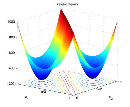
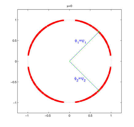
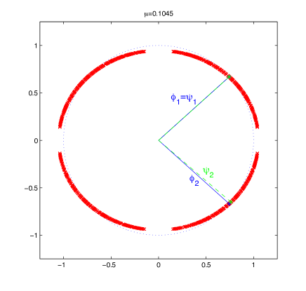
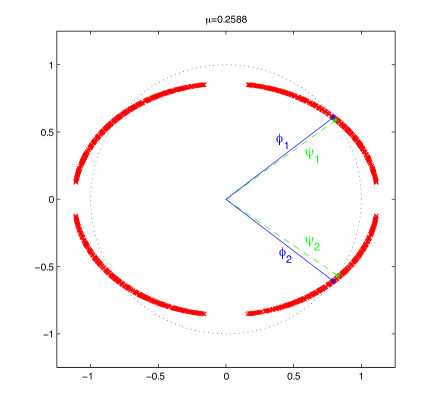
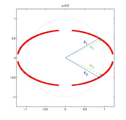
For simplicity and to allow for a visual representation of the outcome it was conducted in . We generated 1000 coefficients by drawing uniformly at random from the interval , setting , randomly permuting the resulting vector and providing it with random signs. We then generated four sets of signals, using four bases with increasing coherence and the same coefficients, and for each set of signals found the minimiser of the K-SVD criterion (1) with . Figure 1 shows the objective function for the case of an orthonormal basis, while Figure 2 shows the four signal sets, the generating bases and the recovered bases. As predicted by our theoretical results when the generating basis is orthogonal it is also the minimiser of the K-SVD criterion, while for an oblique generating basis the minimiser is distorted towards the maximal eigenvector of the basis. Since for a 2-dimensional basis in combination with our coefficient distribution the abstract condition in (35) is always fulfilled, this effect can only be due to the violation of the tightness-condition.
 |
 |
 |
 |
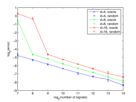
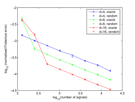
The second experiment illustrates how the local minimum near the generating dictionary approaches the generating dictionary as the number of signals increases. As generating dictionary we choose the union of two orthonormal bases, the Hadamard and the Dirac basis, in dimension , i.e. . We then generated -sparse signals by first drawing uniformly at random from the interval , setting , meaning , and for and then setting for a uniformly at random chosen sign sequence and permutation . We then run the original K-SVD algorithm as described in [3], with a greedy algorithm, and sparsity parameter , using both an oracle initialisation (i.e. the generating dictionary) and a random initialisation, on training sets containing signals for n increasing from 0 to 7. Figure 3 (a) plots the maximal distance between two corresponding atoms of the generating and the learned dictionary, , averaged over 10 runs. Figure 3 (b) is designed to be comparable to the experiment conducted for the noisy -criterion in [22] and plots the normalised Frobenius norm between the generating and the learned dictionary, , averaged over 10 runs.
 |
 |
| (a) | (b) |
As expected we have a log-linear relation between the number of samples and the reconstruction error. However our predictions seem to be too pessimistic. So rather than an inclination of we see one of indicating that . We also see that both the oracle and the random initialisation lead to the same results, raising the question of uniqueness of the equivalent local minima, compare also [22].
5.2 Future work
Finally let us point out further research directions based on a comparison of our results for the K-SVD-minimisation principle to existing identification results. Compared to the available identification results for the -minimisation principle,
| (73) |
it seems at first glance that the
K-SVD-criterion requires a larger sample size than the -criterion, i.e. as opposed to reported in [21] for a basis and reported in [17] for an overcomplete dictionary. Also it does not allow for exact identification with high probability but only guarantees stability. However, this effect may be due to the more general signal model which assumes decay rather than exact sparsity. Indeed it is very interesting to compare our results to a recent result for a noisy version of the -minimisation principle, [22], which provides stability results under unbounded white noise and, omitting log factors, also derives a sampling complexity of .
Another difference, apparently intrinsic to the two minimisation criteria is that probably the K-SVD criterion can only identify tight dictionary frames exactly, while the -criterion allows identification of arbitrary dictionaries. Thus to support the use of the K-SVD criterion for the learning of non-tight dictionaries also theoretically, we plan to study the stability of the K-SVD criterion under non-tightness by analysing the maximal distance between an original, non tight dictionary with condition number and the closest local maximum, cp. also Figure 2.
Compared to identification results for the ER-SpUD algorithm, [37], our results have the advantage of being valid also for overcomplete dictionaries and not exactly sparse signals. The disadvantage is that our results are valid only locally and in case only for a criterion, not an algorithm. An important research direction therefore is to analyse how close the output of K-SVD is to the local minimum of the K-SVD criterion given the same initialisation in the general case.
The last research direction we want to point out is how much decay of the coefficients is actually necessary. For the case , it is quite easy to see, compare also [33, 34], that a condition of the type ensures that the maximal inner product is always attained at . However, typically we have . Therefore a condition such as , which allows for outliers, i.e. signals for which the maximal projection is not at , might be sufficient to prove - if not exact identifiability - at least stability. Together with the inspiring techniques from [22], we expect the tools developed in the course of such an analysis to allow us also to deal with unbounded white noise.
Acknowledgments
This work was supported by the Austrian Science Fund (FWF) under Grant no. Y432 and J3335 and improved thanks to the reviewers’ detailed and pointed comments.
Also I would like to thank Massimo Fornasier for SUPPORT (in capital letters),
Maria Mateescu for proof-reading the proposal leading to grant J3335 and helping me with the shoeshine,
Remi Gribonval for pointing out the connection between an early version of (4) with and K-SVD and
Jan Vybiral for reading several ugly draft versions.
Appendix A Technical details for the proof of Theorem 3.1
Lemma A.1.
For two frames we have
| (74) |
where .
In case is a tight frame with frame constant A and this reduces to
| (75) |
Proof: We have
| (76) |
For each we now split the set of all permutations into disjoint sets , defined as
where is a subset of with and . We then have and
Using these sets we can compute the expectations in (76) as follows
Abbreviating and re-substituting the above expression into (76) leads to,
If is a tight frame and , meaning always has full rank, we have , which leads to the second statement.
Lemma A.2.
Let be a dictionary with isometry constant and be an perturbation of , i.e. . So we can write , where , for and where . Abbreviating , where is the identity matrix in , and , where and , we have
and
whenever is small enough.
In particular when we have
Proof: We first compute the projection in terms of and . Since the matrix is invertible and we can write . We now split into the part contained in the span of and the rest,
| (77) |
Next we calculate . Using the expression in (77) we have
Using the fact that we can estimate
| (78) |
Since this is smaller than 1 for small enough, we can calculate the inverse of using a Neumann series, i.e.
with . This allows us to rewrite as,
| (79) |
and we can estimate
| (80) | ||||
For small enough this is again smaller than and so we can again use a Neumann series to calculate the inverse,
Thus we finally get for the projection onto the perturbed atoms indexed by ,
| (81) |
To calculate up to order we need to keep track of all terms involving up to second order. We have,
| (82) |
and employing the bound for from (A) leads us to,
| (83) |
Similarily we get for ,
Taking into account that the fourth term in the above equation is always smaller than zero we finally get the bound,
| (84) |
Lemma A.3.
For ,
| (85) |
Proof: We have
Since for the last inequality is implied by
which is satisfied as soon as
References
- [1] A. Agarwal, A. Anandkumar, P. Jain, P. Netrapalli, and R. Tandon. Learning sparsely used overcomplete dictionaries via alternating minimization. arXiv:1310.7991, 2013.
- [2] A. Agarwal, A. Anandkumar, and P. Netrapalli. Exact recovery of sparsely used overcomplete dictionaries. arXiv:1309.1952, 2013.
- [3] M. Aharon, M. Elad, and A.M. Bruckstein. K-SVD: An algorithm for designing overcomplete dictionaries for sparse representation. IEEE Transactions on Signal Processing., 54(11):4311–4322, November 2006.
- [4] M. Aharon, M. Elad, and A.M. Bruckstein. On the uniqueness of overcomplete dictionaries, and a practical way to retrieve them. Journal of Linear Algebra and Applications, 416:48–67, July 2006.
- [5] S. Arora, R. Ge, and A. Moitra. New algorithms for learning incoherent and overcomplete dictionaries. arXiv:1308.6273, 2013.
- [6] T. Blumensath and M.E. Davies. Iterative thresholding for sparse approximations. Journal of Fourier Analysis and Applications, 14(5-6):629–654, 2008.
- [7] E. Candès, L. Demanet, D.L. Donoho, and L. Ying. Fast discrete curvelet transforms. Multiscale Modeling & Simulation, 5(3):861–899, 2006.
- [8] E. Candès, J. Romberg, and T. Tao. Robust uncertainty principles: exact signal reconstruction from highly incomplete frequency information. IEEE Transactions on Information Theory, 52(2):489–509, 2006.
- [9] S.S. Chen, D.L. Donoho, and M.A. Saunders. Atomic decomposition by basis pursuit. SIAM Journal on Scientific Computing, 1998.
- [10] O. Christensen. An Introduction to Frames and Riesz Bases. Birkhäuser, 2003.
- [11] I. Daubechies. Ten Lectures on Wavelets. CBMS-NSF Lecture Notes. SIAM, 1992.
- [12] I. Daubechies, R.A. DeVore, M. Fornasier, and S. Güntürk. Iteratively reweighted least squares minimization for sparse recovery. Communications on Pure and Applied Mathematics, 63(1):1–38, January 2010.
- [13] G. Davis, S. Mallat, and M. Avellaneda. Adaptive greedy approximations. Constructive Approximation, 13:57–98, 1997. Springer-Verlag New York Inc.
- [14] D.L. Donoho. Compressed sensing. IEEE Transactions on Information Theory, 52(4):1289–1306, 2006.
- [15] D.L. Donoho, M. Elad, and V.N. Temlyakov. Stable recovery of sparse overcomplete representations in the presence of noise. IEEE Transactions on Information Theory, 52(1):6–18, January 2006.
- [16] D.J. Field and B.A. Olshausen. Emergence of simple-cell receptive field properties by learning a sparse code for natural images. Nature, 381:607–609, 1996.
- [17] Q. Geng, H. Wang, and J. Wright. On the local correctness of -minimization for dictionary learning. arXiv:1101.5672, 2011.
- [18] P. Georgiev, F.J. Theis, and A. Cichocki. Sparse component analysis and blind source separation of underdetermined mixtures. IEEE Transactions on Neural Networks, 16(4):992–996, 2005.
- [19] R. Gribonval, R. Jenatton, F. Bach, M. Kleinsteuber, and M. Seibert. Sample complexity of dictionary learning and other matrix factorizations. arXiv:1312.3790, 2013.
- [20] R. Gribonval, H. Rauhut, K. Schnass, and P. Vandergheynst. Atoms of all channels, unite! Average case analysis of multi-channel sparse recovery using greedy algorithms. Journal of Fourier Analysis and Applications, 14(5):655–687, 2008.
- [21] R. Gribonval and K. Schnass. Dictionary identifiability - sparse matrix-factorisation via -minimisation. IEEE Transactions on Information Theory, 56(7):3523–3539, July 2010.
- [22] R. Jenatton, F. Bach, and R. Gribonval. Local stability and robustness of sparse dictionary learning in the presence of noise. preprint, 2012.
- [23] K. Kreutz-Delgado, J.F. Murray, B.D. Rao, K. Engan, T. Lee, and T.J. Sejnowski. Dictionary learning algorithms for sparse representation. Neural Computations, 15(2):349–396, 2003.
- [24] K. Kreutz-Delgado and B.D. Rao. FOCUSS-based dictionary learning algorithms. In SPIE 4119, 2000.
- [25] M. Ledoux and M. Talagrand. Probability in Banach spaces. Isoperimetry and processes. Springer-Verlag, Berlin, Heidelberg, NewYork, 1991.
- [26] J. Mairal, F. Bach, J. Ponce, and G. Sapiro. Online learning for matrix factorization and sparse coding. Journal of Machine Learning Research, 11:19–60, 2010.
- [27] A. Maurer and M. Pontil. K-dimensional coding schemes in Hilbert spaces. IEEE Transactions on Information Theory, 56(11):5839–5846, 2010.
- [28] N.A. Mehta and A.G. Gray. On the sample complexity of predictive sparse coding. arXiv:1202.4050, 2012.
- [29] D. Needell and J.A. Tropp. CoSaMP: Iterative signal recovery from incomplete and inaccurate samples. Applied Computational Harmonic Analysis, 26(3):301–321, 2009.
- [30] M.D. Plumbley. Dictionary learning for -exact sparse coding. In M.E. Davies, C.J. James, and S.A. Abdallah, editors, International Conference on Independent Component Analysis and Signal Separation, volume 4666, pages 406–413. Springer, 2007.
- [31] DSP Rice University. Compressive sensing resources. http://www.compressedsensing.com/.
- [32] R. Rubinstein, A. Bruckstein, and M. Elad. Dictionaries for sparse representation modeling. Proceedings of the IEEE, 98(6):1045–1057, 2010.
- [33] K. Schnass. Dictionary identification results for K-SVD with sparsity parameter 1. In SampTA13, 2013.
- [34] K. Schnass. On the identifiability of overcomplete dictionaries via the minimisation principle underlying K-SVD. arXiv:1301.3375, 2013.
- [35] K. Schnass and P. Vandergheynst. Average performance analysis for thresholding. IEEE Signal Processing Letters, 14(11):828–831, 2007.
- [36] K. Skretting and K. Engan. Recursive least squares dictionary learning algorithm. IEEE Transactions on Signal Processing, 58(4):2121–2130, April 2010.
- [37] D. Spielman, H. Wang, and J. Wright. Exact recovery of sparsely-used dictionaries. In Conference on Learning Theory (arXiv:1206.5882), 2012.
- [38] J.A. Tropp. Greed is good: Algorithmic results for sparse approximation. IEEE Transactions on Information Theory, 50(10):2231–2242, October 2004.
- [39] J.A. Tropp. On the conditioning of random subdictionaries. Applied Computational Harmonic Analysis, 25(1-24), 2008.
- [40] D. Vainsencher, S. Mannor, and A.M. Bruckstein. The sample complexity of dictionary learning. Journal of Machine Learning Research, 12(3259-3281), 2011.
- [41] R. Vershynin. Introduction to the non-asymptotic analysis of random matrices. In Y. Eldar and G. Kutyniok, editors, Compressed Sensing, Theory and Applications, chapter 5. Cambridge University Press, 2012.
- [42] M. Yaghoobi, T. Blumensath, and M.E. Davies. Dictionary learning for sparse approximations with the majorization method. IEEE Transactions on Signal Processing, 57(6):2178–2191, June 2009.
- [43] M. Zibulevsky and B.A. Pearlmutter. Blind source separation by sparse decomposition in a signal dictionary. Neural Computations, 13(4):863–882, 2001.