Mutual Localization: Two Camera Relative 6-DOF Pose Estimation from Reciprocal Fiducial Observation

Abstract

Concurrently estimating the 6-DOF pose of multiple cameras or robots—cooperative localization—is a core problem in contemporary robotics. Current works focus on a set of mutually observable world landmarks and often require inbuilt egomotion estimates; situations in which both assumptions are violated often arise, for example, robots with erroneous low quality odometry and IMU exploring an unknown environment. In contrast to these existing works in cooperative localization, we propose a cooperative localization method, which we call mutual localization, that uses reciprocal observations of camera-fiducials to obviate the need for egomotion estimates and mutually observable world landmarks. We formulate and solve an algebraic formulation for the pose of the two camera mutual localization setup under these assumptions. Our experiments demonstrate the capabilities of our proposal egomotion-free cooperative localization method: for example, the method achieves 2cm range and 0.7 degree accuracy at 2m sensing for 6-DOF pose. To demonstrate the applicability of the proposed work, we deploy our method on Turtlebots and we compare our results with ARToolKit[1] and Bundler[2], over which our method achieves a tenfold improvement in translation estimation accuracy.

I Introduction

Cooperative localization is the problem of finding the relative 6-DOF pose between robots using sensors from more than one robot. Various strategies involving different sensors have been used to solve this problem. For example, Cognetti et al. [3, 4] use multiple bearning-only observations with a motion detector to solve for cooperative localization among multiple anonymous robots. Trawny et al. [5] and lately Zhou et al. [6, 7] provide a comprehensive mathematical analysis of solving cooperative localization for different cases of sensor data availability. Section II covers related literature in more detail.

To the best of our knowledge, all other cooperative localization works (see Section II) require estimation of egomotion. However, a dependency on egomotion is a limitation for systems that do not have gyroscopes or accelerometers, which can provide displacement between two successive observations. Visual egomotion, like MonoSLAM [8], using distinctive image features estimates requires high quality correspondences, which remains a challenge in machine vision, especially in cases of non-textured environments. Moreover, visual egomotion techniques are only correct upto a scale factor. Contemporary cooperative localization methods that use egomotion [6, 5, 9] yield best results only with motion perpendicular to the direction of mutual observation and fails to produce results when either observer undergoes pure rotation or motion in the direction of observation. Consequently, in simple robots like Turtlebot, this technique produces poor results because of absence of sideways motion that require omni-directional wheels.

To obviate the need for egomotion, we propose a method for relative pose estimation that leverages distance between fiducial markers mounted on robots for resolving scale ambiguity. Our method, which we call mutual localization, depends upon the simultaneous mutual/reciprocal observation of bearing-only sensors. Each sensor is outfitted with fiducial markers (Fig. 1) whose position within the host sensor coordinate system is known, in contrast to assumptions in earlier works that multiple world landmarks would be concurrently observable by each sensor [10]. Since our method does not depend on egomotion, hence it is instantaneous, which means it is robust to false negatives and it do not suffers from the errors in egomotion estimation.

Figure 1: Simplified diagram for the two-camera problem. Assuming the length of respective rays to be $s_{1},s_{2},s_{3},s_{4}$ respectively, each marker coordinates can be written in both coordinate frames $\{p\}$ and $\{q\}$. For example $M_{1}$ is $s_{1}\hat{\mathbf{p}}_{1}$ in frame $\{p\}$ and $\mathbf{q_{1}}$ in $\{q\}$, where $\hat{\mathbf{p}}_{1}$ unit vector parallel to $\mathbf{p}_{1}$.

The main contribution of our work is a generalization of Perspective-3-Points (P3P) problem where observer and the observed points are distributed in different reference frames unlike conventional approach where observer’s reference frame do not contain any observed points and vice versa. In this paper we present an algebraic derivation to solve for the relative camera pose (rotation and translation) of the two bearing-only sensors in the case that each can observe two known fiducial points in the other sensor; essentially giving an algebraic system to compute the relative pose from four correspondences (only three are required in our algorithm but we show how the fourth correspondence can be used to generate a set of hypothesis solutions from which best solution can be chosen). Two fiducial points on each robot (providing four correspondences) are preferable to one on one and two on the other, as it allows extension to multi-robot ($>2$) systems ensuring that any pair of similarly equipped robots can estimate their relative pose. In this paper, we focus on only two robot case as an extension to multi-robot case as pairwise localization is trivial yet practically effective.

Our derivation, although inspired by the linear pose estimation method of Quan and Lan [11], is novel since all relevant past works we know on P3P problem [12], assume all observations are made in one coordinate frame and observed points in the other. In contrast, our method makes no such assumption and concurrently solves the pose estimation problem for landmarks sensed in camera-specific coordinates frames.

We demonstrate the effectiveness of our method, by analyzing its accuracy in both synthetic, which affords quantitative absolute assessment, and real localization situations by deployment on Turtlebots. We use 3D reconstruction experiments to show the accuracy of our algorithm. Our experiments demonstrate the effectiveness of the proposed approach.

II Related Work

Cooperative localization has been extensively studied and applied to various applications. One of the latest works in this area comes from Cognetti et al. [3], [4] where they focus on the problem of cooperatively localizing multiple robots anonymously. They use multiple bearing-only observations and a motion detector to localize the robots. The robot detector is a simple feature extractor that detects vertical cardboard squares mounted atop each robot in the shadow zone of the range finder. One of oldest works come from Karazume et. al. [13] where they focus on using cooperative localization as a substitute to dead reckoning by suggesting a “dance” in which robots act as mobile landmarks. Although they do not use egomotion, but instead assume that position of two robots are known while localizing the third robot. Table I summarizes a few closely related works with emphasis on how our work is different different from each of them. Rest of the section discusses those in detail.

Howard et al. [14] coined the CLAM (Cooperative Localization and Mapping) where they concluded that as an observer robot observes the explorer robot, it improves the localization of robots by the new constraints of observer to explorer distance. Recognizing that odometry errors can cumulate over time, they suggest using constraints based on cooperative localization to refine the position estimates. Their approach, however, do not utilizes the merits of mutual observation as they propose that one robot explores the world and other robot watches. We show in our experiments, by comparison to ARToolKit [1] and Bundler [2], that mutual observations of robots can be up to 10 times more accurate than observations by single robot.

A number of groups have considered cooperative vision and laser based mapping in outdoor environments [15, 16] and vision only [17, 18]. Localization and mapping using heterogeneous robot teams with sonar sensors is examined extensively by [19, 20]. Using more than one robot enables easier identification of previously mapped locations, simplifying the loop-closing problem [21].

Fox et al. [22] propose cooperative localization based on Monte-Carlo localization technique. The method uses odometry measurements for ego motion. Chang et al. [23] uses depth and visual sensors to localize Nao robots in the 2D ground plane. Roumeliotis and Bekey [24] focus on sharing sensor data across robots, employing as many sensors as possible which include odometry and range sensors. Rekleitis et al. [25] provide a model of robots moving in 2D equipped with both distance and bearing sensors.

Related work $\backslash$ Tags	NoEM	BO	NoSLAM	MO
Mutual localization	✓	✓	✓	✓
Howard et al.[14]	✗	✓	✓	✓
Zou and Tan [10]	✓	✓	✗	✗
Cognetti et al.[3]	✗	✓	✓	✗
Trawny et al.[5]	✗	✓	✓	✓
Zhou and Roumeliotis [6, 7]	✗	✓	✓	✓
Roumeliotis et al.[24]	✗	✗	✗	✓

where

Tag meaning NoEM Without Ego-Motion. All those works that use egomotion are marked as  ✗. BO Localization using bearing only measurements. No depth measurements required. All those works that require depth measurements are marked with  ✗. NoSLAM SLAM like tight coupling. Inaccuracy in mapping leads to cumulating interdependent errors in localization and mapping. All those works that use SLAM like approach are marked with a  ✗ MO Utilizes mutual observation, which is more accurate than one-sided observations. All those works that do not use mutual observation, and depend on one-sided observations are marked as  ✗

Table I: Comparison of related work with Mutual localization

Zou and Tan [10] proposed a cooperative simultaneous localization and mapping method, CoSLAM, in which multiple robots concurrently observe the same scene. Correspondences in time (for each robot) and across robots are fed into an extended Kalman filter and used to simultaneously solve the localization and mapping problem. However, this and other “co-slam” approaches such as [26] remain limited due to the interdependence of localization and mapping variables: errors in the map are propagated to localization and vice versa.

Recently Zhou and Roumeliotis [6, 7] have published solution of a set of 14 minimal solutions that covers a wide range of robot to robot measurements. However, they use egomotion for their derivation and they assume that observable fiducial markers coincide with the optical center of the camera. Our work does not make any of the two assumptions.

III Problem Formulation

We use the following notation in this paper, see Fig. 1. $C_{p}$ and $C_{q}$ represent two robots, each with a camera as a sensor. The corresponding coordinate frames are $\{p\}$ and $\{q\}$ respectively with origin at the optical center of the camera. Fiducial markers $M_{1}$ and $M_{2}$ are fixed on robot $C_{q}$ and hence their positions are known in frame $\{q\}$ as $\mathbf{q}_{1},\mathbf{q}_{2}\in\mathbb{R}^{3}$. Similarly, $\mathbf{p}_{3},\mathbf{p}_{4}\in\mathbb{R}^{3}$ are the positions of markers $M_{3}$ and $M_{4}$ in coordinate frame $\{p\}$. Robots are positioned such that they can observe each others markers in their respective camera sensors. The 2D image coordinates of the markers $M_{1}$ and $M_{2}$ in the image captured by the camera $\{p\}$ are measured as $\bar{\mathbf{p}}_{1},\bar{\mathbf{p}}_{2}\in\mathbb{R}^{2}$ and that of $M_{3}$ and $M_{4}$ is $\bar{\mathbf{q}}_{3},\bar{\mathbf{q}}_{4}\in\mathbb{R}^{2}$ in camera $\{q\}$. Let $K_{p},K_{q}\in\mathbb{R}^{3\times 3}$ be the intrinsic camera matrices of the respective camera sensors on robot $C_{p},C_{q}$. Also, note the superscript notation. 2D image coordinates are denoted by a bar, example $\bar{\mathbf{p}}$. Unit vectors that provide bearing information are denoted by a caret, example $\hat{\mathbf{p}}$.

Since the real life images are noisy, the measured image positions $\bar{\mathbf{p}}_{i}$ and $\bar{\mathbf{q}}_{i}$ will differ from the actual positions $\bar{\mathbf{p}}_{i0}$ and $\bar{\mathbf{q}}_{i0}$ by gaussian noise $\mathbf{\eta}_{i}$.

$$\bar{\mathbf{p}}_{i} =\bar{\mathbf{p}}_{i0}+\mathbf{\eta}_{pi} \forall i\in\{1,2\}$$ (1)

$$\bar{\mathbf{q}}_{i} =\bar{\mathbf{q}}_{i0}+\mathbf{\eta}_{qi} \forall i\in\{3,4\}$$ (2)

The problem is to determine the rotation $R\in\mathbb{R}^{3\times 3}$ and translation $\mathbf{t}\in\mathbb{R}^{3}$ from frame $\{p\}$ to frame $\{q\}$ such that any point $\mathbf{p}_{i}$ in frame $\{p\}$ is related to its corresponding point $\mathbf{q}_{i}$ in frame $\{q\}$ by the following equation.

$$\mathbf{q}_{i}=R\mathbf{p}_{i}+\mathbf{t}$$ (3)

The actual projections of markers $M_{i}$ into the camera image frames of the other robot are governed by following equations,

$$\bar{\mathbf{p}}_{i0} =f(K_{p}R^{-1}(\mathbf{q}_{i}-\mathbf{t})) \forall i\in\{1,2\}$$ (4)

$$\bar{\mathbf{q}}_{i0} =f(K_{q}(R\mathbf{p}_{i}+\mathbf{t})) \forall i\in\{3,4\}$$ (5)

where $f$ is the projection function defined over a vector
$\mathbf{v}=\begin{bmatrix}v_{x},v_{y},v_{z}\end{bmatrix}^{\top}$ as

$$f(\mathbf{v})=\begin{bmatrix}\frac{v_{x}}{v_{z}},\frac{v_{y}}{v_{z}}\end{bmatrix}^{\top}$$ (6)

To minimize the effect of noise we must compute the optimal transformation, $R^{*}$ and $\mathbf{t}^{*}$.

$$(R^{*},\mathbf{t}^{*})=\arg\min_{(R,t)}\left(\sum_{i\in\{1,2\}}\|\bar{\mathbf{p}}_{i}-f(K_{p}R^{-1}(\mathbf{q}_{i}-\mathbf{t}))\|^{2}\right.\\ \left.+\sum_{i\in\{3,4\}}\|\bar{\mathbf{q}}_{i}-f(K_{q}(R\mathbf{p}_{i}+\mathbf{t}))\|^{2}\right)$$ (7)

To solve this system of equations we start with exact equations that lead to a large number of polynomial roots. To choose the best root among the set of roots we use the above minimization criteria.

Let $\hat{\mathbf{p}}_{i},\hat{\mathbf{q}}_{i}\in\mathbb{R}^{3}$ be the unit vectors drawn from the camera’s optical center to the image projection of the markers. The unit vectors can be computed from the position of markers in camera images $\bar{\mathbf{p}}_{i},\bar{\mathbf{q}}_{i}$ by the following equations.

$$\hat{\mathbf{p}}_{i} =\frac{K_{p}^{-1}\begin{bmatrix}\bar{\mathbf{p}}_{i}^{\top},1\end{bmatrix}^{\top}}{\|K_{p}^{-1}\begin{bmatrix}\bar{\mathbf{p}}_{i}^{\top},1\end{bmatrix}^{\top}\|} \forall i\in\{1,2\}$$ (8)

$$\hat{\mathbf{q}}_{i} =\frac{K_{q}^{-1}\begin{bmatrix}\bar{\mathbf{q}}_{i}^{\top},1\end{bmatrix}^{\top}}{\|K_{q}^{-1}\begin{bmatrix}\bar{\mathbf{q}}_{i}^{\top},1\end{bmatrix}^{\top}\|} \forall i\in\{3,4\}$$ (9)

Further let $s_{1}$, $s_{2}$ be the distances of markers $M_{1}$, $M_{2}$ from the optical center of the camera sensor in robot $C_{p}$. And $s_{3}$, $s_{4}$ be the distances of markers $M_{3}$, $M_{4}$ from the optical center of camera sensor in robot $C_{q}$. Then the points $\mathbf{q}_{1}$, $\mathbf{q}_{2}$, $s_{3}\hat{\mathbf{q}}_{3}$, $s_{4}\hat{\mathbf{q}}_{4}$ in coordinate frame $\{q\}$ correspond to the points $s_{1}\hat{\mathbf{p}}_{1}$, $s_{2}\hat{\mathbf{p}}_{2}$, $\mathbf{p}_{3}$, $\mathbf{p}_{4}$ in coordinate frame $\{p\}$.

$$\begin{split}\mathbf{q}_{1}&=t+s_{1}R\hat{\mathbf{p}}_{1}\\ \mathbf{q}_{2}&=t+s_{2}R\hat{\mathbf{p}}_{2}\\ s_{3}\hat{\mathbf{q}}_{3}&=t+R\mathbf{p}_{3}\\ s_{4}\hat{\mathbf{q}}_{4}&=t+R\mathbf{p}_{4}\end{split}$$ (10)

These four vector equations provide us 12 constraints (three for each coordinate in 3D) for our 10 unknowns (3 for rotation $R$, 3 for translation $t$, and 4 for $s_{i}$). We first consider only the first three equations, which allows an exact algebraic solution of the nine unknowns from the nine constraints.

Our approach to solving the system is inspired by the well studied problem of Perspective-3-points [12], also known as space resection [11]. However, note that the method cannot be directly applied to our problem as known points are distributed in both coordinate frames as opposed to the space resection problem where all the known points are in the one coordinate frame.

The basic flow steps of our approach are to first solve for the three range factors, $s_{1},s_{2}$ and $s_{3}$ (Section III-A). Then we set up a classical absolute orientation system on the rotation and translation (Section III-B), which is solved using established methods such as Arun et al. [27] or Horn [28]; finally, since our algebraic solution will give rise to many candidate roots, we develop a root-filtering approach to determine the best solution (Section III-C).

III-A Solving for $s_{1}$, $s_{2}$ and $s_{3}$

The first step is to solve the system for $s_{1},s_{2}$ and $s_{3}$. We eliminate $R$ and $t$ by considering the inter-point distances in both coordinate frames.

$$\begin{split}\|s_{1}\hat{\mathbf{p}}_{1}-s_{2}\hat{\mathbf{p}}_{2}\|&=\|\mathbf{q_{1}}-\mathbf{q_{2}}\|\\ \|s_{2}\hat{\mathbf{p}}_{2}-\mathbf{p_{3}}\|&=\|\mathbf{q_{2}}-s_{3}\hat{\mathbf{q}}_{3}\|\\ \|\mathbf{p_{3}}-s_{1}\hat{\mathbf{p}}_{1}\|&=\|s_{3}\hat{\mathbf{q}}_{3}-\mathbf{q_{1}}\|\end{split}$$ (11)

Squaring both sides and representing the vector norm as the dot product gives the following system of polynomial equations.

$$s_{1}^{2}+s_{2}^{2} -2s_{1}s_{2}\hat{\mathbf{p}}_{1}^{\top}\hat{\mathbf{p}}_{2}-\|\mathbf{q}_{1}-\mathbf{q}_{2}\|^{2}=0$$ (12a)

$$s_{2}^{2}-s_{3}^{2} -2s_{2}\hat{\mathbf{p}}_{2}^{\top}\mathbf{p}_{3}+2s_{3}\mathbf{q}_{2}^{\top}\hat{\mathbf{q}}_{3}+\|\mathbf{p}_{3}\|^{2}-\|\mathbf{q}_{2}\|^{2}=0$$ (12b)

$$s_{1}^{2}-s_{3}^{2} -2s_{1}\hat{\mathbf{p}}_{1}^{\top}\mathbf{p}_{3}+2s_{3}\mathbf{q}_{1}^{\top}\hat{\mathbf{q}}_{3}+\|\mathbf{p}_{3}\|^{2}-\|\mathbf{q}_{1}\|^{2}=0$$ (12c)

This system has three quadratic equations implying a Bezout bound of eight ($2^{3})$ solutions. Using the Sylvester resultant we sequentially eliminate variables from each equation. Rewriting (12a) and (12b) as quadratics in terms of $s_{2}$ gives

$$s_{2}^{2}+\underbrace{(-2s_{1}\hat{\mathbf{p}}_{1}^{\top}\hat{\mathbf{p}}_{2})}_{a_{1}}s_{2}+\underbrace{(s_{1}^{2}-|q_{1}-q_{2}|^{2})}_{a_{0}}=0$$ (13)

$$s_{2}^{2}+\underbrace{(-2\hat{\mathbf{p}}_{2}^{\top}\mathbf{p}_{3})}_{b_{1}}s_{2}-\underbrace{(s_{3}^{2}-2s_{3}\mathbf{q}_{2}^{\top}\hat{\mathbf{q}}_{3}-\|\mathbf{p}_{3}\|^{2}+\|\mathbf{q}_{2}\|^{2})}_{b_{0}}=0$$ (14)

The Sylvester determinant [29, p. 123] of (13) and (14) is given by the determinant of the matrix formed by the coefficients of $s_{2}$.

$$r(s_{1},s_{3})=\begin{vmatrix}1&a_{1}&a_{0}&0\\ 0&1&a_{1}&a_{0}\\ 1&b_{1}&b_{0}&0\\ 0&1&b_{1}&b_{0}\end{vmatrix}$$ (15)

This determinant is a quartic function in $s_{1}$, $s_{3}$. By definition of resultant, the resultant is zero if and only if the parent equations have at least a common root[29]. Thus we have eliminated variable $s_{2}$ from (12a) and (12b). We can repeat the process for eliminating $s_{3}$ by rewriting $r(s_{1},s_{3})$ and (12c) as:

$$\begin{split}r(s_{1},s_{3})=c_{4}s_{3}^{4}+c_{3}s_{3}^{3}+c_{2}s_{3}^{2}+c_{1}s_{3}+c_{0}&=0\\ -s_{3}^{2}+\underbrace{(2\mathbf{q}_{1}^{\top}\hat{\mathbf{q}}_{3})}_{d_{1}}s_{3}+\underbrace{s_{1}^{2}-2s_{1}\hat{\mathbf{p}}_{1}^{\top}\mathbf{p}_{3}+\|\mathbf{p}_{3}\|^{2}-\|\mathbf{q}_{1}\|^{2}}_{d_{0}}&=0\end{split}$$ (16)

The Sylvester determinant of (16) would be

$$r_{2}(s_{1})=\begin{vmatrix}c_{4}&c_{3}&c_{2}&c_{1}&c_{0}&0\\ 0&c_{4}&c_{3}&c_{2}&c_{1}&c_{0}\\ 1&d_{1}&d_{0}&0&0&0\\ 0&1&d_{1}&d_{0}&0&0\\ 0&0&1&d_{1}&d_{0}&0\\ 0&0&0&1&d_{1}&d_{0}\end{vmatrix}=0.$$ (17)

Solving (17) gives an 8 degree polynomial in $s_{1}$. By Abel-Ruffini theorem [30, p. 131], a closed-form solution of the above polynomial does not exist.

The numeric solution to (17) gives eight roots for $s_{3}$. We compute $s_{1}$ and $s_{2}$ using (12c) and (12b) respectively. Because the camera cannot see objects behind it, only real positive roots are maintained from the resultant solution set.

III-B Solving for $R$ and $t$

With the solutions for the scale factors, $\{s_{1},s_{2},s_{3}\}$ we can compute the absolute location of the Markers $\{M_{1},M_{2},M_{3}\}$ in both the frames $\{p\}$ and $\{q\}$.

$$\mathbf{p}_{i}=s_{i}\hat{\mathbf{p}}_{i} \forall i\in\{1,2\}$$

$$\mathbf{q}_{i}=s_{i}\hat{\mathbf{q}}_{i} \forall i\in\{3\}$$

These exact correspondences give rise to the classical problem of absolute orientation i.e. given three points in two coordinate frames find the relative rotation and translation between the frames. For each positive root of $s_{1}$, $s_{2}$, $s_{3}$ we use the method in Arun et. al [27] method (similar to Horn’s method [28]) to compute the corresponding rotation $R$ and translation value $\mathbf{t}$.

III-C Choosing the optimal root

Completing squares in (12) yields important information about redundant roots.

$$(s_{1}+s_{2})^{2} -2s_{1}s_{2}(1+\hat{\mathbf{p}}_{1}^{\top}\hat{\mathbf{p}}_{2})-\|\mathbf{q}_{1}-\mathbf{q}_{2}\|^{2}=0$$ (18a)

$$(s_{2}-\hat{\mathbf{p}}_{2}^{\top}\mathbf{p}_{3})^{2}-(s_{3}-\mathbf{q}_{2}^{\top}\hat{\mathbf{q}}_{3})^{2}\\ +(\mathbf{p}_{3}-\hat{\mathbf{p}}_{2})^{\top}\mathbf{p}_{3}-\mathbf{q}_{2}^{\top}(\mathbf{q}_{2}-\hat{\mathbf{q}}_{3})=0\\$$ (18b)

$$(s_{1}-\hat{\mathbf{p}}_{1}^{\top}\mathbf{p}_{3})^{2}-(s_{3}-\mathbf{q}_{1}^{\top}\hat{\mathbf{q}}_{3})^{2}\\ +(\mathbf{p}_{3}-\hat{\mathbf{p}}_{1})^{\top}\mathbf{p}_{3}-\mathbf{q}_{1}^{\top}(\mathbf{q}_{1}-\hat{\mathbf{q}}_{3})=0\\$$ (18c)

Equations (18) do not put any constraints on positivity of terms $(s_{2}-\hat{\mathbf{p}}_{2}^{\top}\mathbf{p}_{3})$, $(s_{3}-\mathbf{q}_{2}^{\top}\hat{\mathbf{q}}_{3})$, $(s_{1}-\hat{\mathbf{p}}_{1}^{\top}\mathbf{p}_{3})$ or $(s_{3}-\mathbf{q}_{1}^{\top}\hat{\mathbf{q}}_{3})$. However, all these terms are positive as long as the markers of the observed robot are farther from the camera than the markers of the observing robot. Also, the distances $s_{i}$ are assumed to be positive. Assuming the above, we filter the real roots by the following criteria:

$$s_{1} \geq\|\mathbf{p}_{3}\|$$ (19)

$$s_{2} \geq\|\mathbf{p}_{3}\|$$ (20)

$$s_{3} \geq\max(\|\mathbf{q}_{1}\|,\|\mathbf{q}_{2}\|)$$ (21)

These criteria not only reduce the number of roots significantly, but also filter out certain degenerate cases.

For all the filtered roots of (17), we compute the corresponding values of $R$ and $\mathbf{t}$, choosing the best root that minimizes the error function, (7).

III-D Extension to more than three markers

Even though the system is solvable by only three markers, we choose to use four markers for symmetry. We can fall back to the three marker solution in situations when one of the markers is occluded. Once we extend this system to 4 marker points, we obtain 6 bivariate quadratic equations instead of the three in (12) that can be reduced to three 8-degree univariate polynomials. The approach to finding the root with the least error is the same as described above.

The problem of finding relative pose from five or more markers is better addressed by solving for the homography when two cameras observe the same set of points as done by [31, 32, 33, 34]. The difference for us is that the distance between the points in both coordinate frames is known hence we can estimate the translation metrically which is not the case in classical homography estimation. Assuming the setup for five points such that (10) becomes

$$\begin{split}\mathbf{q}_{1}&=t+s_{1}R\hat{\mathbf{p}}_{1}\\ \mathbf{q}_{2}&=t+s_{2}R\hat{\mathbf{p}}_{2}\\ s_{3}\hat{\mathbf{q}}_{3}&=t+R\mathbf{p}_{3}\\ s_{4}\hat{\mathbf{q}}_{4}&=t+R\mathbf{p}_{4}\\ s_{5}\hat{\mathbf{q}}_{5}&=t+R\mathbf{p}_{5}\end{split}$$ (22)

If the essential matrix is $E$, the setup is the same as solving for

$$[\mathbf{q}_{1},\mathbf{q}_{2},\hat{\mathbf{q}}_{3},\hat{\mathbf{q}}_{4},\hat{\mathbf{q}}_{5}]^{\top}E[\hat{\mathbf{p}}_{1},\hat{\mathbf{p}}_{2},\mathbf{p}_{3},\mathbf{p}_{4},\mathbf{p}_{5}]=0$$ (23)

The scale ambiguity of the problem can be resolved by one of the distance relations from (11). Please refer to [32] for solving (23). For more points refer to [35] for the widely known 7-point and linear 8-point algorithms.

IV Implementation

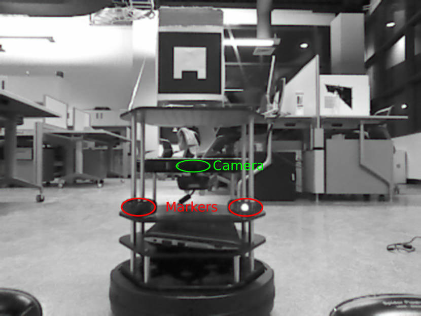
Figure 2: The deployment of markers on Turtlebot that we used for our experiments

We implement our algorithm on two Turtlebots with fiducial markers. One of the Turtlebots with markers is shown in Fig. 2. We have implemented the algorithm in Python using the Sympy [36], OpenCV [37] and Numpy [38] libraries. As the implementing software formulates and solves polynomials symbolically, it is generic enough to handle any reasonable number of points in two camera coordinate frames. We have tested the solver for the following combination of points: 0-3, 1-2, 2-2, where 1-2 means that 1 point is known in the first coordinate frame and 2 points are known in the second.

We use blinking lights as fiducial markers on the robots and barcode-like cylindrical markers as for the 3D reconstruction experiment.

The detection of blinking lights follows a simple thresholding strategy on the time differential of images. This approach coupled with decaying confidence tracking produces satisfactory results for simple motion of robots and relatively static backgrounds. Fig. 3 shows the cameras mounted with blinking lights as fiducial markers. The robots shown in 3 are also mounted with ARToolKit[1] fiducial markers for the comparison experiments.

V Experiments

Figure 3: Diagram of the two camera setup for mutual localization 3D metric reconstruction, along with images from each camera for two poses of the mobile camera. Cameras have distinctive cylindrical barcode-like markers to aid detection in each others image frames. Also depicted is the triangulation to two example feature points.

To assess the accuracy of our method we perform a localization experiment in which we measure how accurately our method can determine the pose of the other camera. We compare our localization results with the widely used fiducial-based pose estimation in ARToolKit [1] and visual egomotion and SfM framework Bundler [2]. We also generate a semi-dense reconstruction to compare the mapping accuracy of our method to that of Bundler. A good quality reconstruction, is a measure of the accuracy of mutual localization of the two cameras used in the reconstruction.

V-A Localization Experiment

Setup

Two turtlebots were set up to face each other. One of the turtlebot was kept stationary and the other moved in 1 ft increments in an X-Z plane (Y-axis is down, Z-axis is along the optical axis of the static camera and the X-axis is towards the right of the static camera). We calculate the rotation error by extracting the rotation angle from the differential rotation $R_{gt}^{\top}R_{est}$ as follows:

$$E_{\theta}=\frac{180}{\pi}\arccos\left(\frac{\operatorname{Tr}(R_{gt}^{\top}R_{est})-1}{2}\right)$$ (24)

where $R_{gt}$ is the ground truth rotation matrix, $R_{est}$ is the estimated rotation matrix and $\operatorname{Tr}$ is the matrix trace. The translation error is simply the norm difference between two translation vectors.

Results in comparison with ARToolKit [1]

The ARToolKit is an open source library for detecting and determining the pose of fiducial markers from video. We use a ROS[39] wrapper – ar_pose – over ARToolKit for our experiments. We repeat the relative camera localization experiment with the ARToolKit library and compare to our results. The results show a tenfold improvement in translation error over Bundler[2].

	Median Trans. error	Median Rotation error
ARToolKit[1]	0.57m	$9.2^{\circ}$
Bundler[2]	0.20m	$0.016^{\circ}$
Mutual Localization	0.016m	$0.33^{\circ}$

Table II: Table showing mean translation and rotation error for ARToolKit, Bundler and Mutual Localization

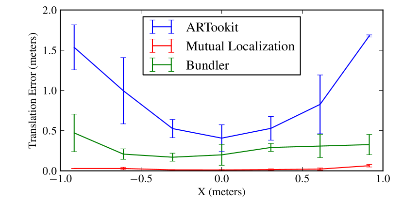
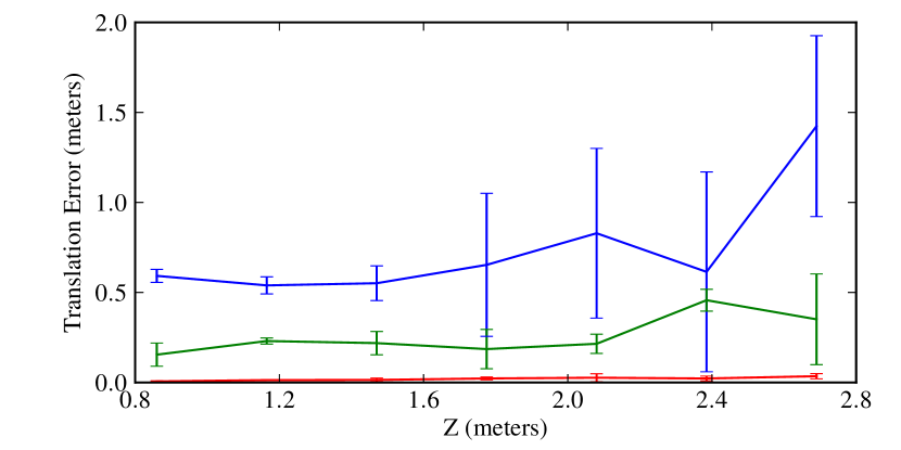
Figure 4: Translation error comparison between the ARToolKit and our mutual localization. The translation error is plotted to ground truth X and Z axis positions to show how error varies with depth (Z) and lateral (X) movements. We get better results in localization by a factor of ten. Also note how the translation error increases with Z-axis (inter-camera separation).

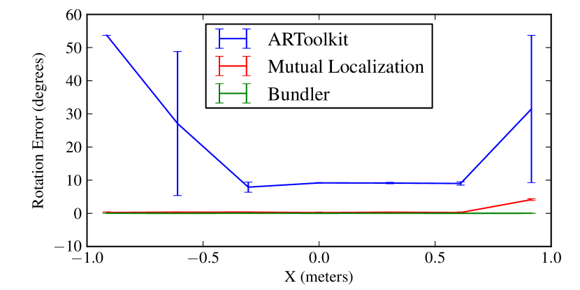
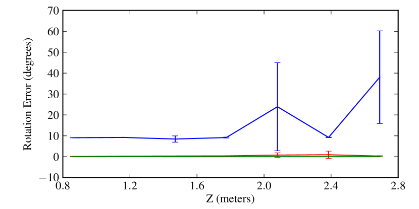
Figure 5: Rotation error comparison between the ARToolKit and Mutual localization. Rotation error decreases with Z-axis (ground truth inter-camera separation). See (24) for computation of rotation error.

V-B Simulation experiments with noise

A simple scene was constructed in Blender to verify the mathematical correctness of the method. Two cameras were set up in the blender scene along with a target object 1m from the static camera. Camera images were rendered at a resolution of 960 $\times$ 540. The markers were simulated as colored balls that were detected by simple hue based thresholding. The two cameras in the simulated scene were rotated and translated to cover maximum range of motion. After detection of the center of the colored balls, zero mean gaussian noise was added to the detected positions to investigate the noise characteristics of our method. The experiment was repeated with different values of noise covariance. Fig 6 shows the translation and rotation error in the experiment with variation in noise. It can be seen that our method is robust to noise as it deviates only by 5cm and $2.5^{\circ}$ when tested with noise of up to 10 pixels.

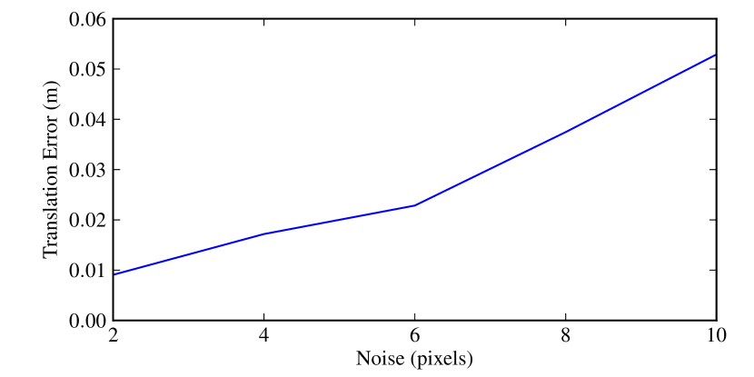
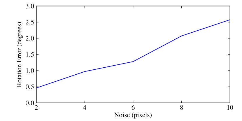
Figure 6: Rotation and translation error as noise is incrementally added to the detection of markers.

V-C 3D Reconstruction experiment

The position and orientation obtained from our method is inputted into the patch based multi-view stereo (PMVS-2) library [40] to obtain a semi-dense reconstruction of an indoor environment. Our reconstruction is less noisy when compared to that obtained by Bundler [2]. Fig. 7 shows a side-by-side snapshot of the semi-dense map from Bundler-PMVS and, our method, Mutual Localization-PMVS. To compare the reconstruction accuracy, we captured the scene as a point cloud with an RGB-D camera (Asus-Xtion). The Bundler and Mutual Localization output point clouds were manually aligned (and scaled) to the Asus-Xtion point cloud. We then computed the nearest neighbor distance from each point in the Bundler/Mutual localization point clouds discarding points with nearest neighbors further than 1m as outliers. With this metric the mean nearest neighbor distance for our method was 0.176m while that for Bundler was 0.331m.

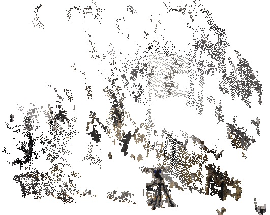
(a) Bundler-PMVS

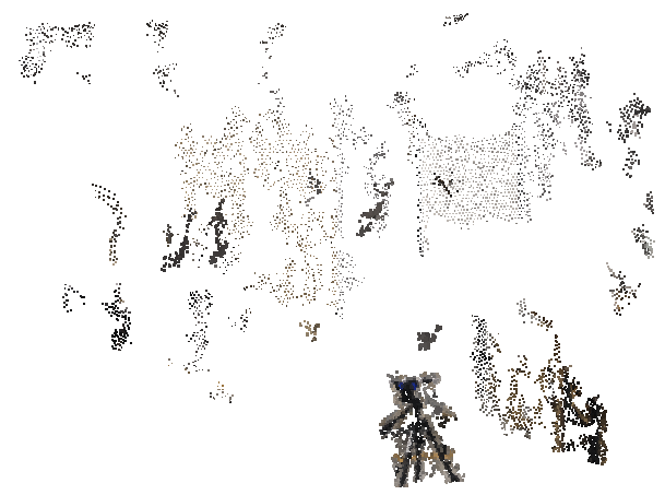
(b) Mutual Localization-PMVS

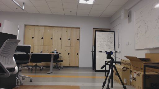
(c) Actual scene

Figure 7: The semi-dense reconstruction produced by our method, Mutual Localization, is less noisy (0.18m) when compared to that produced by Bundler (0.33m).

VI Conclusion

We have developed a method to cooperatively localize two cameras using fiducial markers on the cameras in sensor-specific coordinate frames, obviating the common assumption of sensor egomotion. We have compared our results with the ARToolKit showing that our method can localize significantly more accurately, with a tenfold error reduction observed in our experiments. We have also demonstrated how the cooperative localization can be used as an input for 3D reconstruction of unknown environments, and find better accuracy (0.18m versus 0.33m) than the visual egomotion-based Bundler method. We plan to build on this work and apply it to multiple robots for cooperative mapping. Though we achieve reasonable accuracy, we believe we can improve the accuracy of our method by improving camera calibration and measurement of the fiducial marker locations with respect to the camera optical center. We will release the source code (open-source) for our method upon publication.

References

- [1] H. Kato and M. Billinghurst, “Marker tracking and HMD calibration for a video-based augmented reality conferencing system,” in Proceedings of the 2nd IEEE and ACM International Workshop on Augmented Reality (IWAR 99), Oct 1999.
- [2] N. Snavely, S. Seitz, and R. Szeliski, “Photo tourism: exploring photo collections in 3D,” in ACM Transactions on Graphics (TOG), vol. 25, no. 3. ACM, 2006, pp. 835–846.
- [3] M. Cognetti, P. Stegagno, A. Franchi, G. Oriolo, and H. Bulthoff, “3-D mutual localization with anonymous bearing measurements,” in Robotics and Automation (ICRA), 2012 IEEE International Conference on, may 2012, pp. 791 –798.
- [4] A. Franchi, G. Oriolo, and P. Stegagno, “Mutual localization in a multi-robot system with anonymous relative position measures,” in Intelligent Robots and Systems, 2009. IROS 2009. IEEE/RSJ International Conference on. IEEE, 2009, pp. 3974–3980.
- [5] N. Trawny, X. Zhou, K. Zhou, and S. Roumeliotis, “Interrobot transformations in 3-D,” Robotics, IEEE Transactions on, vol. 26, no. 2, pp. 226–243, 2010.
- [6] X. S. Zhou and S. I. Roumeliotis, “Determining the robot-to-robot 3D relative pose using combinations of range and bearing measurements: 14 minimal problems and closed-form solutions to three of them,” in Intelligent Robots and Systems (IROS), 2010 IEEE/RSJ International Conference on. IEEE, 2010, pp. 2983–2990.
- [7] ——, “Determining 3-D relative transformations for any combination of range and bearing measurements,” Robotics, IEEE Transactions on, vol. PP, no. 99, pp. 1–17, 2012.
- [8] A. J. Davison, I. D. Reid, N. D. Molton, and O. Stasse, “Monoslam: Real-time single camera slam,” Pattern Analysis and Machine Intelligence, IEEE Transactions on, vol. 29, no. 6, pp. 1052–1067, 2007.
- [9] A. Martinelli, “Vision and IMU data fusion: Closed-form solutions for attitude, speed, absolute scale, and bias determination,” Robotics, IEEE Transactions on, no. 99, pp. 1–17, 2012.
- [10] D. Zou and P. Tan, “CoSLAM: Collaborative visual SLAM in dynamic environments,” IEEE Transactions on Pattern Analysis and Machine Intelligence, 2012.
- [11] L. Quan and Z. Lan, “Linear n-point camera pose determination,” Pattern Analysis and Machine Intelligence, IEEE Transactions on, vol. 21, no. 8, pp. 774–780, 1999.
- [12] B. Haralick, C. Lee, K. Ottenberg, and M. Nölle, “Review and analysis of solutions of the three point perspective pose estimation problem,” International Journal of Computer Vision, vol. 13, no. 3, pp. 331–356, 1994.
- [13] R. Kurazume, S. Nagata, and S. Hirose, “Cooperative positioning with multiple robots,” in Robotics and Automation, 1994. Proceedings., 1994 IEEE International Conference on, may 1994, pp. 1250 –1257 vol.2.
- [14] A. Howard and L. Kitchen, “Cooperative localisation and mapping,” in International Conference on Field and Service Robotics (FSR99). Citeseer, 1999, pp. 92–97.
- [15] R. Madhavan, K. Fregene, and L. Parker, “Distributed cooperative outdoor multirobot localization and mapping,” Autonomous Robots, vol. 17, pp. 23–39, 2004.
- [16] J. Ryde and H. Hu, “Mutual localization and 3D mapping by cooperative mobile robots,” in Proceedings of International Conference on Intelligent Autonomous Systems (IAS), The University of Tokyo, Tokyo, Japan, Mar. 2006.
- [17] J. Little, C. Jennings, and D. Murray, “Vision-based mapping with cooperative robots,” in Sensor Fusion and Decentralized Control in Robotic Systems, vol. 3523, October 1998, pp. 2–12.
- [18] R. Rocha, J. Dias, and A. Carvalho, “Cooperative multi-robot systems: a study of vision-based 3-D mapping using information theory,” Robotics and Autonomous Systems, vol. 53, pp. 282–311, April 2005.
- [19] R. Grabowski and P. Khosla, “Localization techniques for a team of small robots,” in Proceedings of the IEEE/RSJ International Conference on Intelligent Robots and Systems (IROS), 2001.
- [20] P. Khosla, R. Grabowski, and H. Choset, “An enhanced occupancy map for exploration via pose separation,” in Proceedings of the IEEE/RSJ International Conference on Intelligent Robots and Systems (IROS), 2003.
- [21] K. Konolige and S. Gutmann, “Incremental mapping of large cyclic environments,” International Symposium on Computer Intelligence in Robotics and Automation (CIRA), pp. 318–325, 2000.
- [22] D. Fox, W. Burgard, H. Kruppa, and S. Thrun, “Collaborative multi-robot localization,” in KI-99: Advances in Artificial Intelligence, ser. Lecture Notes in Computer Science, W. Burgard, A. Cremers, and T. Cristaller, Eds. Springer Berlin / Heidelberg, 1999, vol. 1701, pp. 698–698.
- [23] C.-H. Chang, S.-C. Wang, and C.-C. Wang, “Vision-based cooperative simultaneous localization and tracking,” in Robotics and Automation (ICRA), 2011 IEEE International Conference on, may 2011, pp. 5191 –5197.
- [24] S. Roumeliotis and G. Bekey, “Distributed multirobot localization,” Robotics and Automation, IEEE Transactions on, vol. 18, no. 5, pp. 781 – 795, oct 2002.
- [25] L. M. Rekleitis, G. Dudek, and E. E. Milios, “Multi-robot exploration of an unknown environment, efficiently reducing the odometry error,” in In Proc. of the International Joint Conference on Artificial Intelligence (IJCAI), 1997, pp. 1340–1345.
- [26] G.-H. Kim, J.-S. Kim, and K.-S. Hong, “Vision-based simultaneous localization and mapping with two cameras,” in Intelligent Robots and Systems, 2005. (IROS 2005). 2005 IEEE/RSJ International Conference on, aug. 2005, pp. 1671 – 1676.
- [27] K. Arun, T. Huang, and S. Blostein, “Least-squares fitting of two 3-D point sets,” Pattern Analysis and Machine Intelligence, IEEE Transactions on, no. 5, pp. 698–700, 1987.
- [28] B. Horn, “Closed-form solution of absolute orientation using unit quaternions,” JOSA A, vol. 4, no. 4, pp. 629–642, 1987.
- [29] V. Bykov, A. Kytmanov, M. Lazman, and M. Passare, Elimination methods in polynomial computer algebra. Kluwer Academic Pub, 1998, vol. 448.
- [30] E. Barbeau, Polynomials, ser. Problem Books in Mathematics. Springer, 2003.
- [31] H. Stew nius, C. Engels, and D. Nist r, “Recent developments on direct relative orientation,” ISPRS Journal of Photogrammetry and Remote Sensing, vol. 60, no. 4, pp. 284 – 294, 2006. [Online]. Available: http://www.sciencedirect.com/science/article/pii/S092427160600030X
- [32] D. Nister, “An efficient solution to the five-point relative pose problem,” Pattern Analysis and Machine Intelligence, IEEE Transactions on, vol. 26, no. 6, pp. 756–770, 2004.
- [33] J. Philip, “A non-iterative algorithm for determining all essential matrices corresponding to five point pairs,” The Photogrammetric Record, vol. 15, no. 88, pp. 589–599, 1996. [Online]. Available: http://dx.doi.org/10.1111/0031-868X.00066
- [34] H. Longuet-Higgins, “A computer algorithm for reconstructing a scene from two projections,” Readings in Computer Vision: Issues, Problems, Principles, and Paradigms, MA Fischler and O. Firschein, eds, pp. 61–62, 1987.
- [35] R. Hartley and A. Zisserman, Multiple view geometry in computer vision. Cambridge Univ Press, 2000, vol. 2.
- [36] O. Certik et al., “Sympy python library for symbolic mathematics,” Technical report (since 2006), http://code. google. com/p/sympy/(accessed November 2009), Tech. Rep., 2008.
- [37] G. Bradski, “The opencv library,” Doctor Dobbs Journal, vol. 25, no. 11, pp. 120–126, 2000.
- [38] N. Developers, “Scientific computing tools for python-numpy,” 2010.
- [39] M. Quigley, B. Gerkey, K. Conley, J. Faust, T. Foote, J. Leibs, E. Berger, R. Wheeler, and A. Ng, “ROS: an open-source robot operating system,” in ICRA workshop on open source software, vol. 3, no. 3.2, 2009.
- [40] Y. Furukawa and J. Ponce, “Accurate, dense, and robust multiview stereopsis,” Pattern Analysis and Machine Intelligence, IEEE Transactions on, vol. 32, no. 8, pp. 1362–1376, 2010.