Exploring the non-linear density field in the Millennium simulations with tessellations – I. The probability distribution function

Abstract

We use the Delaunay Tessellation Field Estimator (DTFE) to study the one-point density distribution functions of the Millennium (MS) and Millennium-II (MS-II) simulations. The DTFE technique is based directly on the particle positions, without requiring any type of smoothing or analysis grid, thereby providing high sensitivity to all non-linear structures resolved by the simulations. In order to identify the detailed origin of the shape of the one-point density probability distribution function (PDF), we decompose the simulation particles according to the mass of their host FoF halos, and examine the contributions of different halo mass ranges to the global density PDF. We model the one-point distribution of the FoF halos in each halo mass bin with a set of Monte Carlo realizations of idealized NFW dark matter halos, finding that this reproduces the measurements from the N-body simulations reasonably well, except for a small excess present in simulation results. This excess increases with increasing halo mass. We show that its origin lies in substructure, which becomes progressively more abundant and better resolved in more massive dark matter halos. We demonstrate that the high density tail of the one-point distribution function in less massive halos is severely affected by the gravitational softening length and the mass resolution. In particular, we find these two parameters to be more important for an accurate measurement of the density PDF than the simulated volume. Combining our results from individual halo mass bins we find that the part of the one-point density PDF originating from collapsed halos can nevertheless be quite well described by a simple superposition of a set of NFW halos with the expected cosmological abundance over the resolved mass range. The transition region to the low-density unbound material is however not well captured by such an analytic halo model.

1 Introduction

One of the most important questions in cosmology is to understand the formation of large-scale structures in the Universe. In the standard $\Lambda$CDM model, the energy density of today’s Universe is dominated by non-baryonic cold dark matter ($\sim 23\%$) and dark energy ($\sim 73\%$), whereas only $\sim 4\%$ is comprised of all the mass and energy associated with planets, stars, galaxies, clusters, gas, dust and electromagnetic radiation. The study of large scale structures is hence primarily the study of the distribution of galaxies and the underlying dark matter.

The distribution of galaxies can be well studied with large galaxy redshift surveys (e.g. SDSS Stoughton et al. (2002), or 2dFGRS Colless et al. (2001)) which provide maps of the distribution of galaxies over large volumes in the (mostly) nearby Universe. On the other hand, there is no direct detection of dark matter particles yet and its existence is mostly inferred from indirect observations such as gravitational lensing, making its observational study much harder. In the current paradigm of structure formation, structures form via gravitational instability amplifying tiny density fluctuations generated by some process in the early Universe. These initial density fluctuations are often assumed to form a Gaussian random field. Dark matter first aggregates hierarchically into dark matter halos and galaxies form later in their centres by the cooling and condensation of baryons (White & Rees, 1978). As the dark matter halos form near peaks of the initial density field, the distribution of dark matter and galaxies on large scales is largely determined by the statistics of these peaks (Bardeen et al., 1986). On small scales, the physics of galaxy formation complicates this picture considerably, leading to non-linear and stochastic biasing between the distributions of dark matter and galaxies.

Studies of the cosmic density field expected in cold dark matter cosmologies are often based on simple and approximate analytical models such as the halo model (Cooray & Sheth, 2002). However, detailed studies of the non-linear cosmic density field need to rely on N-body simulations, which do not need to make simplifying assumptions about the abundance and structure of halos. In the present work, we study the non-linear density fields predicted by high-resolution dark matter simulations, particularly the one-point probability distribution function of the dark matter density field. We measure this function far into the nonlinear regime and compare the results to the halo model.

The output of N-body simulations provides the phase space distribution of dark matter particles. Reconstructing the underlying continuous density field represented by the discrete set of “macro-particles” used by the numerical scheme requires one to define an appropriate density reconstruction scheme. For consistency, we demand that the total mass contained in the reconstructed continuous density field has to be exactly equal to the total mass represented by the discrete set of particles. There exist various techniques in the literature for density reconstruction from a given set of points which fulfill these requirements (Hockney & Eastwood, 1981; Silverman, 1986; Monaghan, 1992; Ascasibar & Binney, 2005). The most widely used approach is to convolve the point data with some filtering function (or simply ‘kernel’), yielding a continuous map. Conventionally, the filtering function has a fixed shape and fixed size (for example when binning particles on a regular grid by CIC or TSC mass assignment), but this fixed smoothing technique has the serious disadvantage that the smoothing length is not adjusted to clustering of the particle distribution. So when a small smoothing length is employed in order to achieve great resolving power in high density regions like filaments and clusters, these structure are well recovered but underdense regions like voids are severely affected by shot noise. Conversely, if one wishes to obtain a reasonable reconstruction of low-density voids by using a larger smoothing length, the filaments and clusters are oversmoothed, limiting the amount of information that can be extracted from those regions.

A better smoothing technique is obtained by applying the SPH (smoothed particle hydrodynamics) approach, where one employs an adaptive kernel which adjusts itself according to the varying sampling density. For example, the size of the (compact) kernel can be set to the distance of the $n$-th nearest neighbor, where the value of $n$ is a user-specified parameter. In both of these methods, the smoothing kernel has to be specified by the user. Common choices consist of spherically symmetric kernels, for example a simple Gaussian. However, the fact that the geometry of the kernel is prescribed irrespective of anisotropies present in local non-linear structures (e.g. filaments and sheets) may introduce spurious topological signatures characteristic of the kernel. Ideally, one would like to allow the point distribution to decide for itself what kernel shape and size yields the most faithful reconstruction of the local density field. An ideal candidate for this strategy is the Voronoi tessellation and/or its topological dual, the Delaunay tessellation (van de Weygaert, 1994; Okabe et al., 2000; Pelupessy et al., 2003; van de Weygaert, 2007; Schaap, 2007). The density estimators based on these tessellations have several advantages over the traditional smoothing techniques which we discuss in the next section. These advantages of DTFE over traditional smoothing techniques for density reconstruction have made it an increasingly popular choice in recent years (e.g. Aragón-Calvo et al. 2007, Zhang et al. 2010, Platen et al. 2011). We will primarily use the Delaunay tessellation field estimator (DTFE) because it offers a parameter free reconstruction of the density field, retaining a maximum amount of information about the density field and the topology of structures embedded in the dark matter distribution.

The Millennium Simulation (hereafter MS) (Springel et al., 2005) is still one of the largest high-resolution simulations of the growth of dark matter structures. It followed the evolution of $10$ billion dark matter particles in a $500\,h^{-1}{\rm Mpc}$ comoving box with an individual particle mass of $8.61\times 10^{8}\,h^{-1}\,M_{\odot}$. The Millennium-II simulation (hereafter MS-II ; Boylan-Kolchin et al. 2009) simulated a $100\,h^{-1}{\rm Mpc}$ box using the same number of particles, thereby offering $125$ times better mass resolution. Boylan-Kolchin et al. (2009) studied the formation and statistics of dark matter halos in the MS-II simulation. By comparing their results with the MS simulation they found excellent convergence in the basic dark matter halo statistics, making these two simulations ideally suited for a study of the dark matter density field over an unprecedented range of scales.

The one point distribution function of the cosmological density field is one of most fundamental quantities characterizing statistical properties of the matter distribution in the Universe. In the current paradigm of structure formation, the present day large scale structures grew from primordial density fluctuations with Gaussian statistics. The one point distribution of today’s density field is however far from Gaussian as a result of gravitational evolution. In the mildly non-linear regime, it is known that the one point distribution of the dark matter density field obtained from N-body simulations is reasonably well described by a log-normal distribution (Coles & Jones, 1991; Kofman et al., 1994; Kayo et al., 2001; Taruya et al., 2003), but this approximation eventually breaks down in the highly non-linear regime.

In this paper, we study the one point distribution of the dark matter density fields in the MS and MS-II using DTFE and try to interpret the results in the simple picture provided by the halo model. The dark matter halos are the densest sites in the cosmic mass density field, and approximately $\sim 50\%$ ($49.6\%$ in the MS and $\gtrsim 60\%$ in the MS-II at $z=0$, with a $20$ particle limit) of the mass is bound in resolved halos. Note that in the halo model, all of the mass in the Universe is assumed to be part of a dark matter halo of some mass. The density profiles of simulated CDM halos are well described by the universal NFW profile (Navarro et al., 1996), with a shape approximately independent of mass, the amplitude of initial density fluctuations and cosmology (Navarro et al., 1997; Cole & Lacey, 1996; Jing, 2000). The concentration varies weekly with halo formation time. In the halo model, one tries to represent the underlying dark matter distribution as a superposition of a set of NFW halos with abundance and clustering modelled with simplistic models or analytic fits to N-body results.

N-body simulations compute a periodic model universe of finite size and finite mass resolution. This also requires a softening length below which the gravitational interaction is suppressed to avoid singularities in orbit integrations and unphysical particle scattering. These numerical limitations are expected to influence the ability of the simulation to resolve very high and very low density regions, and consequently affect the tails of the one-point distribution. The MS and MS-II use different simulation volumes, mass resolutions and softening lengths, allowing us to study the importance of these effects in shaping the tails of the one-point distributions. We note that the use of a user defined kernel for estimating densities like in SPH introduces a smoothing scale and a corresponding resolution element which will typically have an additional effect on the tails of the distribution. As DTFE is self-adaptive without a free parameter, this type of effect is expected to be less important for this scheme than other numerical limitations due to finite volume, finite mass resolution and gravitational softening.

This paper is structured as follows. In Section 2, we outline the Delaunay Field Tessellation Estimator and discuss our methodology. We then present results for toy halo models and the MS and MS-II simulations in Section 3. Finally we conclude and summarize our findings in Section 4.

2 Density estimation with the DTFE

In mathematics and computational geometry, the Delaunay tessellation for a set of points is the uniquely defined volume-covering tessellation with mutually disjoint tetrahedra, in which no circumsphere of any tetrahedron contains one of the points in its interior (Delaunay, 1934; Okabe et al., 2000). Connecting the centers of the circumscribed spheres of neighboring Delaunay tetrahedra produces the Voronoi tessellation of the point set, which is the topological dual of the Delaunay tessellation. The Voronoi tessellation is a division of space into non overlapping convex regions where each region is uniquely assigned to one of the sampling points. All the points in these convex regions are closer to its defining sampling point than to any other sampling point.

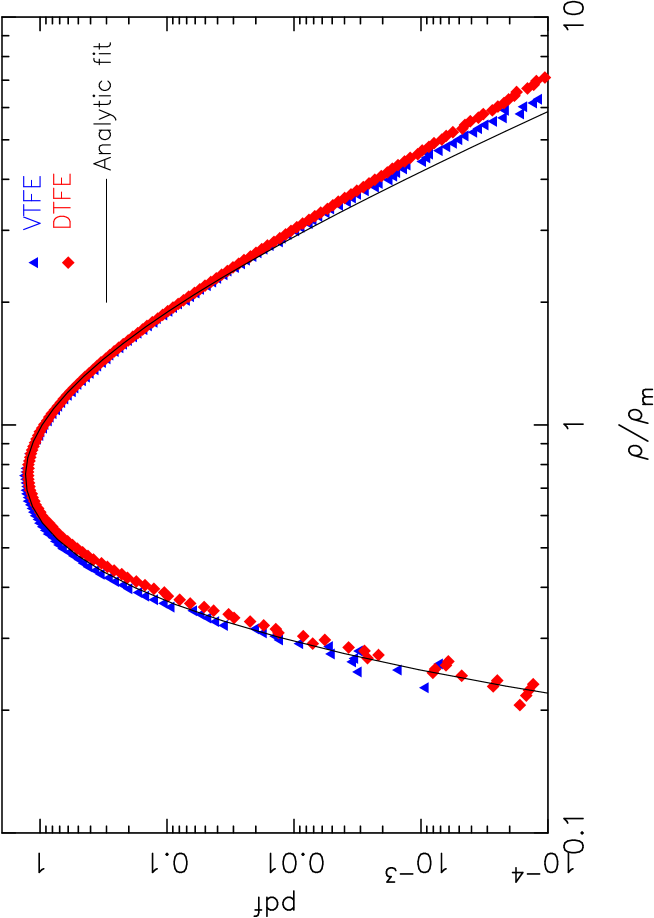
Figure 1: The probability distribution functions of VTFE and DTFE reconstructed density fields for a Poisson point process with $10^{6}$ particles in 3D. The one-point distribution function in each bin is weighted by the bin width and the volume weighted density in that bin. An analytic approximation for the VTFE reconstructed density field given by Eqn. (3) is shown as a solid line. The corresponding best fit values $a$, $b$, and $c$ for VTFE and DTFE are listed in Table 1.

Estimator	VTFE	DTFE
$N$	$1000000$	$6772467$
$a$	$368.56\pm 10.75$	$536.76\pm 6.96$
$b$	$7.97\pm 0.05$	$8.31\pm 0.016$
$c$	$6.03\pm 0.031$	$6.35\pm 0.012$

Table 1: The number of points $N$, and the fitting parameters $a$, $b$ and $c$ assuming a functional form $f(\tilde{\rho})=a\,\tilde{\rho}^{-b}\,e^{-c/\tilde{\rho}}$ for the PDF of VTFE and DTFE reconstructed density fields for a 3D Poisson point processes. The mean is $1$ for both PDFs. The variances of the PDFs of VTFE and DTFE are $0.22$ and $0.24$ respectively.

Based on the geometric constructions of these tessellations, different density reconstruction schemes can be constructed. For example, the density at each sampling point in the VTFE (Voronoi Tessellation Field Estimator) is simply defined as $\rho_{i}={\,m_{i}}/{V_{i}}$, where $m_{i}$ is the mass of the $i$-th sampling point and $V_{i}$ is the volume of the corresponding Voronoi cell. This method assumes that the mass of each particle is uniformly distributed inside each Voronoi cell, keeping the density constant inside each cell. The product of density and volume of all the Voronoi cells trivially returns exactly the total mass of all the sampling points. But an important deficiency of this density reconstruction is that the density field is discontinuous at the Voronoi cell boundaries.

An improved density estimator that addresses this deficit is the Delaunay Tessellation Field Estimator (DTFE), which is based on a Delaunay tessellation of the sampling points, as proposed by Schaap & van de Weygaert (2000). Here the density at each sampling point is defined as $\rho_{i}={4\,m_{i}}/{W_{i}}$ where $W_{i}$ is the volume of the contiguous Delaunay region around the point (composed of all the tetrahedra that have the point as one of their vertices). The sum $W_{i}=\sum_{j}V_{ij}^{\rm Del}$ is the sum of the volumes of all Delaunay tetrahedra that share point $i$ as one of their vertices. The multiplication by $4$ accounts for the fact that each Delaunay tetrahedron is contributing to the contiguous Delaunay region of four points. The DTFE density estimation scheme assumes that the density field inside each tetrahedron varies in a linear fashion. The gradient of the density is assumed to be constant within each tetrahedron and can then be computed using the density values at the four vertices of the tetrahedron. One can then easily find the density at any other location inside the tetrahedron using tri-linear interpolation. This creates a continuous, volume covering, piece-wise linear density field. It is easy to verify that the volume integral of the DTFE density field reproduces the sum of the particle masses exactly. The most important advantage of DTFE over conventional methods is that the density estimates in this method do not rely on any additional parameter. The DTFE kernel not only adapts to the local density as in the case of SPH but also to the local geometry of the distribution. We employ the tessellation engine of the parallel AREPO code (Springel, 2010) to construct the Delaunay mesh.

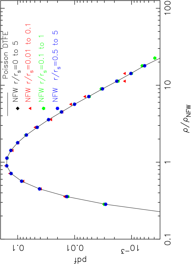
Figure 2: Distributions of ${\rho}/{\rho_{\rm NFW}}$ for all the particles within $r_{200}$ in an NFW halo with parameters $M_{200}=10^{6}\,{\rm M}_{\odot}$, $N_{200}=10^{6}$, $r_{200}=50\,{\rm kpc}$ and $c=5$ (black symbols). The distributions for particles residing within certain radial ranges are separately shown, as indicated in the figure. Note that the distributions shown in this plot are simply the histograms, and their values in each bin are not weighted by the bin width or the volume weighted density as in Figure 1. The distributions in different radial bins are all of the same shape and are consistent with what we obtained for the Poisson sampling of a uniform distribution, even though the sampling densities vary strongly across the different radial bins.

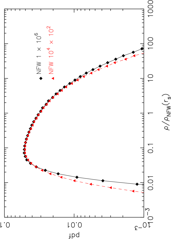
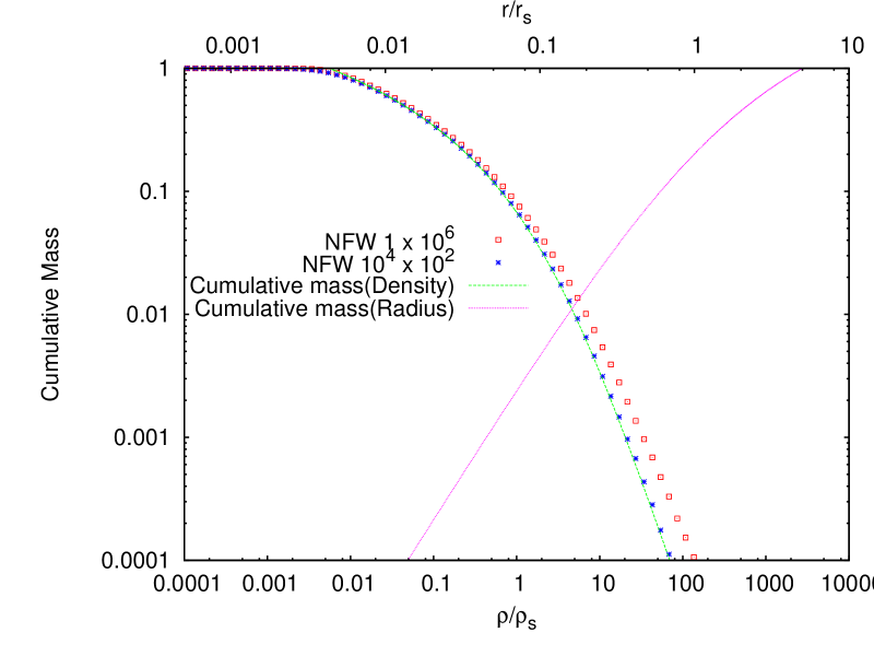
Figure 3: The top panel compares the distributions of ${\rho}/{\rho_{\rm NFW}(r_{s})}$ for all particles in a NFW halo with parameters $M_{200}=10^{6}\,{\rm M}_{\odot}$, $N_{200}=10^{6}$, $r_{200}=50\,{\rm kpc}$, $c=5$, and in all the $10^{4}$ halos with $M_{200}=10^{6}\,{\rm M}_{\odot}$, $N_{200}=10^{2}$, $r_{200}=50\,{\rm kpc}$, $c=5$. The bottom panel shows the cumulative mass as a function of density in the halo. The results show that the DTFE can quite reliably represent the mass profile of the entire halo even with a particle number as low as $N_{200}=10^{2}$. The overprediction of the cumulative mass at $r<r_{s}$ in the $N_{200}=10^{6}$ halo is caused by contributions from other radii due to large scatter in the DTFE densities.

To construct and store the Delaunay mesh, AREPO uses indices to refer to $4$ vertices and $4$ adjacent tetrahedra of each tetrahedron which requires at least $32$ bytes of memory per tetrahedron on $64$-bit machines (plus 4 bytes for an auxiliary variable in practice), provided the number of points per distributed memory region is kept low enough to allow the use of 32-bit integers (which is the case in practice). For a random point set there are on average $\sim 6.77$ tetrahedra per point (van de Weygaert, 1994), implying at least $\sim 244$ bytes of memory per point for storing the mesh tetrahedra. Another $20$ bytes per point are required to hold the particle coordinates (if stored in single precision) and a unique particle ID. In practice, additional memory is needed for a search tree (in order to validate individual Delaunay tetrahedra by efficiently searching for points inside the circumsphere) and for ‘ghost’ cells that mesh the different tessellation patches together across processor domains. There are more than $10$ billion particles in both MS and in MS-II. This requires us to build a Delaunay tessellation composed of more than $70$ billion tetrahedra for each of these simulations. We used the ODIN machine at the Computing Center of the Max Planck Society, Garching, to perform the mesh constructions for MS and MS-II, using $512$ cores and $\sim 7.5$ Terabytes of memory in total. In both cases, the mesh construction took about $20$ minutes of wall-clock time.

3 Results

In cosmology, we quite often encounter Poisson sampling of an underlying density field. For example, the galaxies in a redshift survey or the particles in an N-body simulation can be considered as Poisson samples for certain density ranges. Therefore it is important to understand the impact of the Poisson sampling noise on the statistics of the reconstructed density distribution. Both the VTFE and the DTFE reconstruct the density field with an adaptive spatial resolution from a discrete set of data points. The high sensitivity of these density estimators to the variation of local density and geometry makes them presumably particularly sensitive to the presence of shot noise. We therefore first examine the statistical properties of Poisson sampling noise as seen by these density estimators. Further, the datasets in cosmology also often involve Poisson sampling of highly inhomogeneous distributions for example from N-body simulations and galaxy surveys. It is also important to test whether the one point distribution for uniform Poisson sampling of a homogeneous distribution also describes the noise caused by Poisson sampling an inhomogeneous distribution. We address this question with Monte Carlo simulations of NFW halos.

We start this section by characterising the performance of the DTFE for a Poisson sample (in Subsection 3.1) and for Monte Carlo realisations of NFW halos (in Subsection 3.2). These test cases, for which the underlying continuous density field is known, will help us to understand and interpret the main results of the paper, the one point density distributions of the cosmic density field given by the DTFE applied on the Millennium simulations (in Subsection 3.3). We finalise this section by examining the impact in our results of halo substructure and ellipticity, as well as of numerical setup of the simulations.

3.1 Density PDF of a 3D Poisson point process

We begin by studying the one-point distribution function of the density for a Poisson process analyzed with Voronoi tessellations. A Poisson Voronoi tessellation results when the generating points of the Voronoi cells are a Poisson point sampling of a uniform field. In the case of one-dimensional Voronoi tessellations, one can rigorously derive the probability distribution of the lengths of the segments, which is given by

$$g(\tilde{x})=4\,\tilde{x}\,\exp(-2\,\tilde{x}),$$ (1)

where $\tilde{x}={l}/{\left<l\right>}$. Here $l$ is the length of the Voronoi cell and $\left<l\right>$ its average. No analytical results are known for the size distributions of Poisson Voronoi cells in 2D and 3D. Empirical studies using Monte Carlo realizations fit the distribution of surface area or volume of the Voronoi cells in 2D or 3D with a gamma type probability distribution function (Kiang, 1966) approximated by

$$g(\tilde{x};a)=\frac{a^{a}}{\Gamma(a)}\tilde{x}^{a-1}e^{-a\,\tilde{x}},$$ (2)

where $\tilde{x}={v}/{\left<v\right>}$ is the size of the Voronoi cell in units of the average cell size, $0\geq\tilde{x}\geq\infty$, and $a$ is a constant whose value depends on the dimensionality of the space. Monte Carlo experiments suggest $a=2$, $4$ and $6$, for 1D, 2D and 3D, respectively.

The probability of a random point to lie inside a Voronoi cell of size $\tilde{x}$ is the product of $g(\tilde{x})$ and $\tilde{x}$, which in other words is the probability of a random point to have a density $\tilde{\rho}={1}/{\tilde{x}}$ in the VTFE reconstructed density field. Following this definition, the one point distribution function of the VTFE reconstructed density field in 3D is

$${\rm d}g(\tilde{\rho})=dg(\tilde{x})\times\tilde{x}=388.8\,\tilde{\rho}^{-8}\,e^{-6/\tilde{\rho}}\,{\rm d}\tilde{\rho},$$ (3)

if the hypothesis that $g(\tilde{x};a)$ follows equation (2) with $a=6$ is indeed correct. To verify these results, we generate a Poisson point process with $10^{6}$ points in a cubic box $100\,h^{-1}\,{\rm Mpc}$ on a side. We construct the Voronoi tessellation and Delaunay tessellation of the points and then estimate the density field values at the sampling points using both VTFE and DTFE. We compute the one point distribution of both the VTFE and DTFE reconstructed density fields. We use only the density estimates at the sampling points for computing the one-point distribution of the VTFE reconstructed density field, and determine the best-fit parameters assuming a functional form $f(\tilde{\rho})=a\,\tilde{\rho}^{-b}\,e^{-c/\tilde{\rho}}$ to describe the one-point PDF of the VTFE reconstructed density field. In the VTFE density reconstruction scheme, the density at the location of the sampling points is defined as the inverse of the volume of its corresponding Voronoi cell weighted by its mass, whereas in the DTFE scheme the volumes of the contiguous Delaunay cells are used instead.

In the DTFE density reconstruction, the density field inside each tetrahedron varies linearly, whereas in the VTFE density reconstruction the density inside each Voronoi cell is constant. To account for this difference and arrive at a more appropriate comparison between DTFE and VTFE, we randomly select one point inside each Delaunay tetrahedron through uniform sampling and determine its density estimate by linearly interpolating from the four vertices of the corresponding tetrahedron. We weight each such point by the volume of the corresponding tetrahedron. We also weight each point in VTFE by the volume of their Voronoi cells. As there are on average $\sim 6.77$ Delaunay tetrahedra per point for a random data set (van de Weygaert, 1994), we get $6772467$ density estimates from the DTFE reconstructed density field by randomly choosing one point from each tetrahedron. The one-point distributions of the VTFE and DTFE reconstructed density fields are both fitted to the same functional form of equation (3) and the best-fit parameters are listed in Table 1. We find that the distributions obtained for the VTFE density field are well described by equation (3), and the values of our best-fit parameters approach the literature values as the number of particles is increased. The distribution obtained for the DTFE density field is pretty similar overall, but it is clearly not exactly the same. Both for the VTFE and DTFE reconstructions, equation (3) noticeably underpredicts the high density tail of the one-point distribution function. It is also interesting that the two schemes have very similar variances despite the seemingly larger smoothing involved in the DTFE scheme.

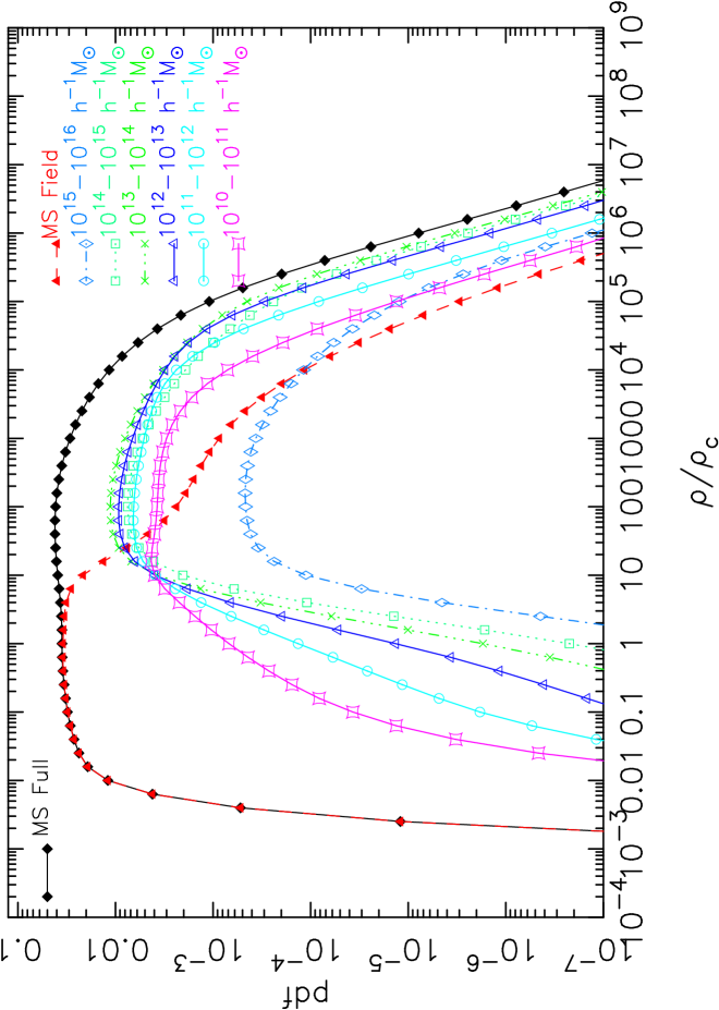
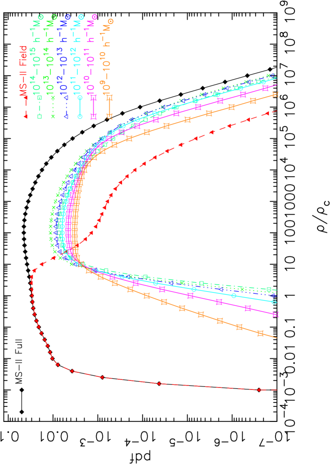
Figure 4: The left and right panels show the density distributions constructed with DTFE for the MS and the MS-II, respectively. After computing the DTFE density for all the particles, we identify the particles residing in FoF halos of different mass ranges, and the particles which do not reside in any halo, and then compute the density distribution for each of the components separately. The distributions for non member particles and for particles in different halo mass bins are shown with different colours and symbols (as indicated in the panels) together with the distribution for all the particles (black squares).

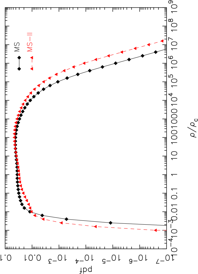
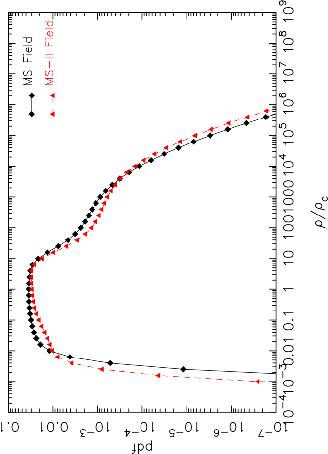
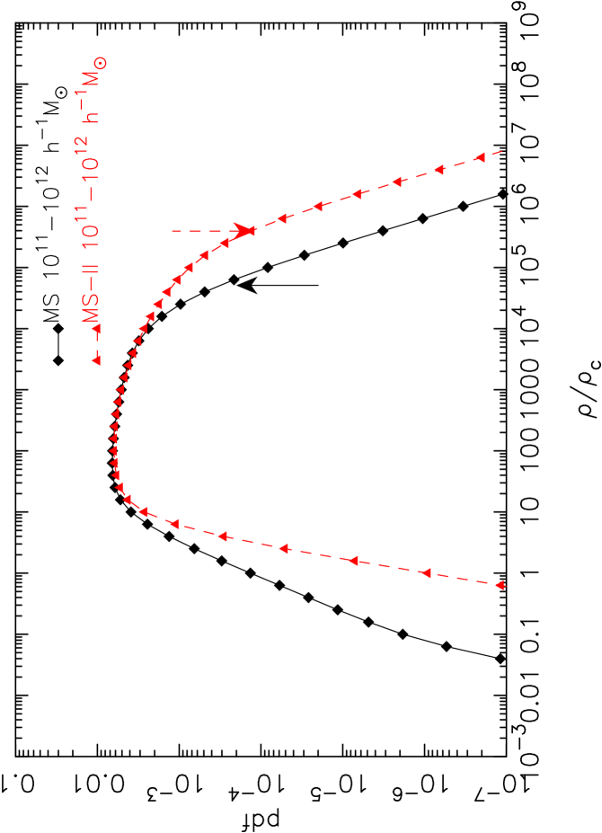
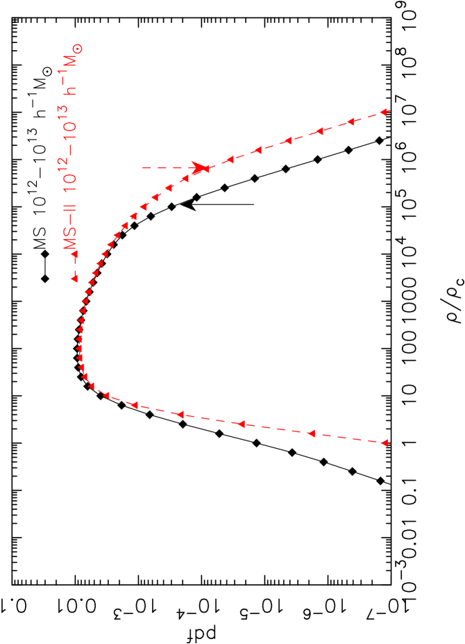
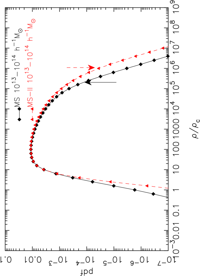
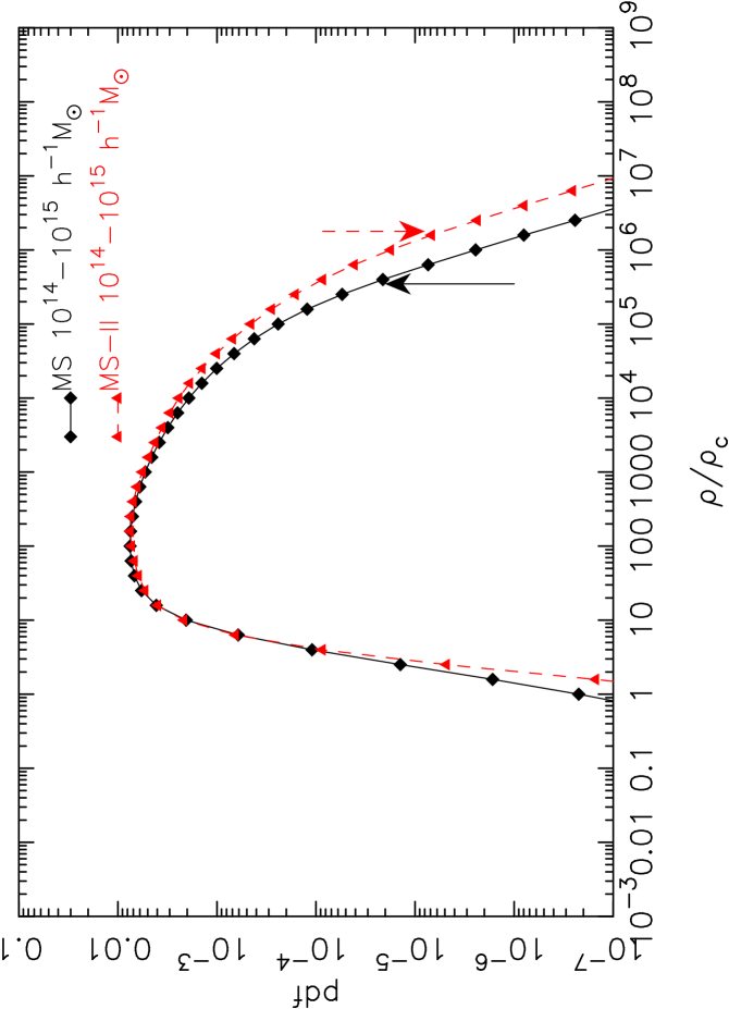
Figure 5: Comparison of DTFE density distributions for all the particles, all the non-halo particles, and all the particles in different halo mass bins in MS and MS II. The bottom four panels show different halo mass ranges, as labeled. The arrows in each panel show the density corresponding to the softening radius in MS and MS-II for each mass bin. The top left shows all the components together (i.e. all the particles in the simulations) while the top right compares only the non-halo particles.

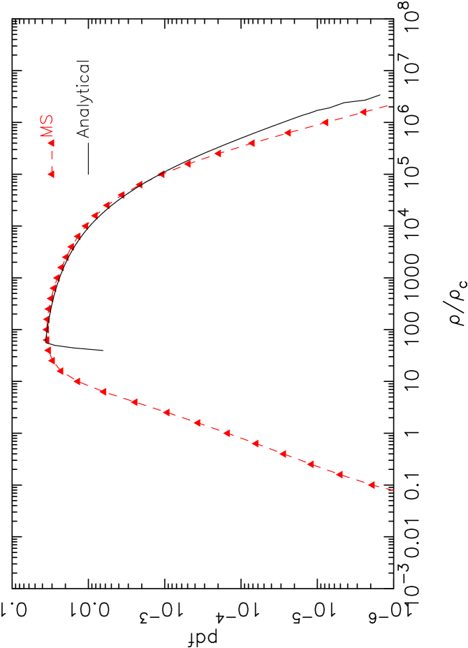
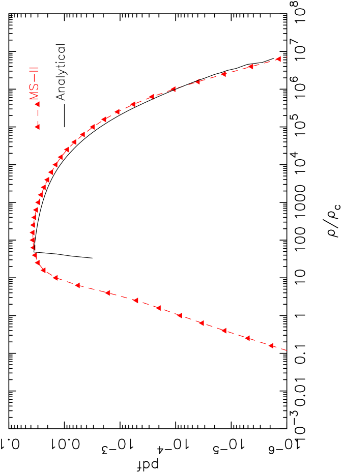
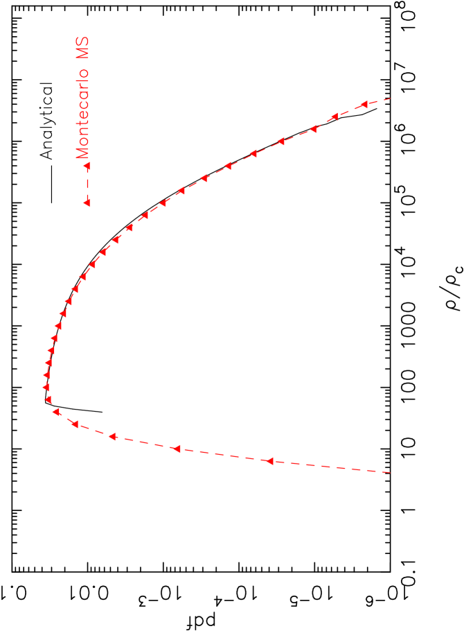
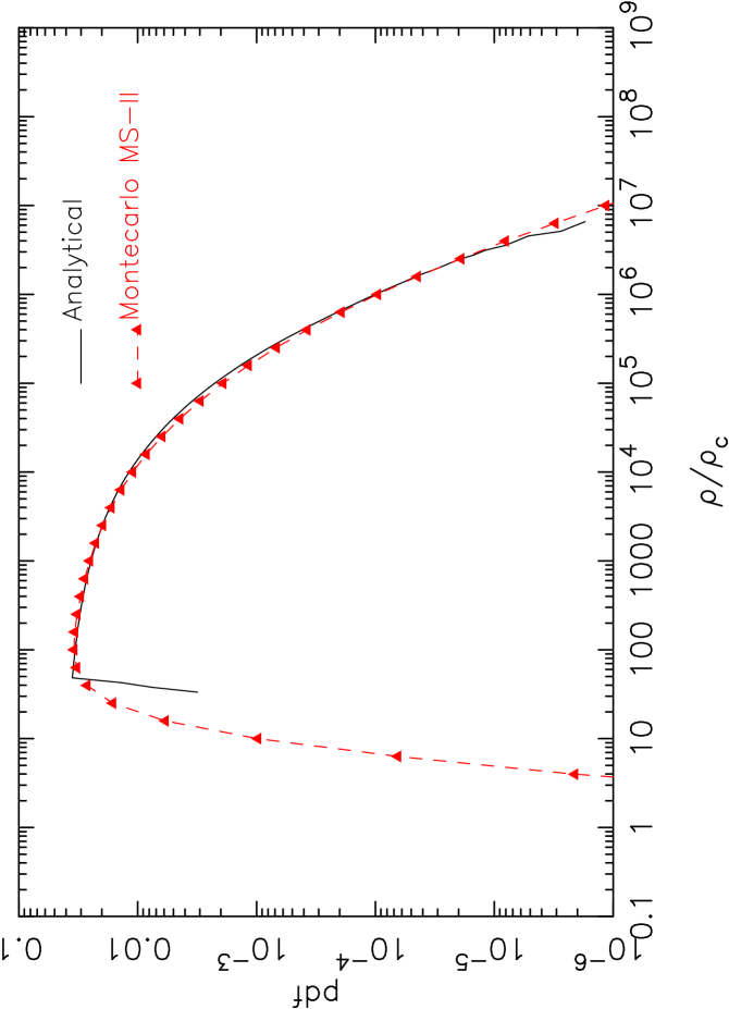
Figure 6: Comparison of our analytical halo model predictions for the one-point distribution of the density with the direct numerical simulation results summed over an equal range of halo mass bins (top row), or with the similarly summed Monte Carlo realizations of NFW halos over the same mass range (bottom row). For the MS we carry out the sum over $5$ equally spaced different halo mass bins, each spanning a decade in the halo mass range $10^{11}-10^{16}\,h^{-1}M_{\sun}$. Similarly, for MS-II the sum is carried out over $6$ equally spaced different halo mass bins in the halo mass range $10^{9}-10^{15}\,h^{-1}M_{\sun}$. In both cases, we show results for the MS (left panels) and the MS-II (right panels) as red dashed lines, while the analytical halo model is shown with solid black lines.

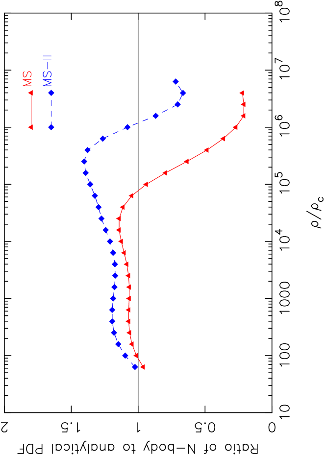
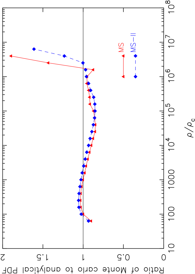
Figure 7: Same as Fig. 6, but here we show the ratios of the one-point distribution obtained from N-body simulations to our analytical halo model predictions (left panel), and similarly for Monte Carlo realizations of NFW halos relative to our analytical halo model predictions (right panel).

3.2 Monte Carlo realizations of NFW halos

Dark Matter halos in N-body simulation are highly inhomogeneous systems which we idealize as systems with spherical NFW density profile (Navarro et al., 1996, 1997).

The NFW density profile is given by

$$\rho(r)=\frac{\rho_{c}\,\delta_{c}}{\frac{r}{r_{s}}\,\left(1+\frac{r}{r_{s}}\right)^{2}},$$ (4)

corresponding to a cumulative mass within radius $r$ of

$$M(r)=\int_{0}^{r}4\pi r^{\prime 2}\rho(r^{\prime})\,{\rm d}r^{\prime}=4\pi\rho_{c}\delta_{c}r_{s}^{3}\left[\ln(1+\tfrac{r}{r_{s}})-\tfrac{{r}/{r_{s}}}{1\,+\,{r}/{r_{s}}}\right].\\$$ (5)

Here $\rho_{c}={3H_{0}^{2}}/({8\pi G})$ is the critical density, $r_{s}={r_{200}}/{c}$ is the scale radius, $r_{200}$ is the virial radius, $c$ is the concentration of the halo, and $\delta_{c}$ is the characteristic density. The virial mass of the halo is $M_{200}=200\,\rho_{c}\,(4\pi/3)\,r_{200}^{3}$. The characteristic density

$$\delta_{c}=\frac{200}{3}\,\frac{c^{3}}{\ln(1+c)-{c}/{(1+c)}}$$ (6)

is related to the concentration $c$ by the requirement that the mean density within $r_{200}$ should be $200$ times the critical density.

To generate our mock NFW halos, we first specify $M_{200}$ and the particle mass. This determines the number $N_{200}$ of particles which reside within $r_{200}$. Next, we specify the concentration of the halo using the mass-concentration relation determined from the Millennium Simulation by Neto et al. (2007). We then populate the halo with particles using a Monte Carlo sampling technique, i.e. the probability to place a particle at a certain radius is made proportional to ${\rm d}M$ from equation (5). This is augmented with isotropically selected angular co-ordinates $\theta$ and $\phi$. To avoid boundary effects, we extend the NFW halo radially out to $3\,r_{200}$.

3.2.1 One-point distribution in different parts of the same halo

We generate Monte Carlo realizations of an NFW halo with the following parameters: $M_{200}=10^{6}{\rm M}_{\odot}$, $N_{200}=10^{6}$, $r_{200}=50\,{\rm kpc}$ and $c=5$. The halo extends out to $3\times r_{200}$. We put the halo at the center of a cubic box with a side of length $6\times r_{200}$ and construct the Delaunay tessellation using all the particles in the halo. Note that this leaves empty regions at the corners of the box. The Delaunay cells near the halo boundary will then be very extended due to the presence of these empty regions resulting in spurious density estimates. In order to avoid these boundary effects we limit our analysis to the particles residing within the virial radius $r_{200}$ of the halo. We choose three radial bins, ${r}/{r_{s}}=0.01-0.1$, ${r}/{r_{s}}=0.1-1$ and ${r}/{r_{s}}=0.5-5$, in order to probe different regimes of sampling density. We identify all the particles residing in these radial ranges and compute the ratio of the DTFE estimate of density to the NFW expected value for each particle in each radial bin. The results for the three different radial bins together with that for all the particles within $r_{200}$ are shown in Figure 2. Despite the fact that the different radial bins have different sampling density, the one-point distributions in different radial bins are all the same and are consistent with that obtained for a Poisson point sampling of a uniform distribution.

3.2.2 Dependence on mass resolution

Halos identified in N-body simulations (or galaxy groups found in surveys) consist of different numbers of particles. In order to understand how the one-point distribution of DTFE reconstructed density fields depends on the number of particles used to resolve them, we generate a set of five NFW halos each with the same parameters $M_{200}=10^{6}{\rm M}_{\odot}$, $r_{200}=50{\rm kpc}$ and $c=5$, but with different numbers of particles: $N_{200}=10^{6}$, $10^{5}$, $10^{4}$, $10^{3}$, and $10^{2}$, respectively. The one-point distribution function of the DTFE reconstructed density field of a $N_{200}=10^{2}$ halo will be noisier compared to a $N_{200}=10^{6}$ halo due to effects of discreteness. In order to take the discreteness effects into account we generate different numbers of NFW halos for each resolution: $1$ with $N_{200}=10^{6}$, $10$ with $N_{200}=10^{5}$, $10^{2}$ with $N_{200}=10^{4}$, $10^{3}$ with $N_{200}=10^{3}$ and $10^{4}$ with $N_{200}=10^{2}$ particles. One then has same total number of density estimates for each resolution, allowing a straightforward comparison of the one-point distribution functions at the same noise level.

In the top panel of Figure 3, we show the one-point distribution of ${\rho}/{\rho_{\rm NFW}(r_{s})}$ for all the particles within $r_{200}$ for NFW halos with $N_{200}=10^{6}$ and $N_{200}=10^{2}$ particles. The distributions look very similar, except that the high density tail of the distribution for the $N_{200}=10^{2}$ halo shows a slight shift towards lower density as compared to the $N_{200}=10^{6}$ halo.

We also compute the cumulative mass fractions as a function of density from the distributions of the $N_{200}=10^{2}$ and $N_{200}=10^{6}$ halos, and compare them in the bottom panel of Figure 3. The theoretical prediction is shown with a solid line. This quantity gives the fraction of the virial mass contained when the NFW density profile is integrated from the center of the halo up to a certain density. The cumulative mass fraction as a function of radius is also shown, by indicating the radius along the $x$-axis on top. Interestingly, the plot shows that even with $N_{200}=100$ one can quite reliably reproduce the cumulative mass fraction from the measured one-point density distribution of the NFW halo. The $N_{200}=10^{6}$ halo overpredicts the cumulative mass at $\rho>\rho_{s}$ which roughly corresponds to $r<{r_{s}}/{2}$. This overprediction is related to the large scatter in the DTFE density estimates which causes a broad range of radii in the halo to contribute to any individual density bin. Furthermore, the range of radii contributing to a density bin becomes even broader near the center of the halo due to the shallower profile of the inner region. The core of the $N_{200}=10^{6}$ halos are resolved better relative to the halos sampled with $N_{200}=10^{2}$. The halos with $N_{200}=10^{2}$ particles tend to underestimate the densities near the center. Here the boost due to scatter in densities is somewhat compensated by the poor resolution, enabling it to nicely but arguably misleadingly recover the analytic mass profile even near the center of the halo.

3.3 The one-point distribution function in the Millennium and Millennium-II simulations

In the halo model, it is assumed that all the matter in the Universe resides in a halo of some mass. With this assumption, the whole matter distribution can be represented as a superposition of a set of halos in different mass ranges. To define the model one only needs to specify the density profiles of halos and the halo mass function. The density profile of dark matter halos can be described by the NFW profile (equation 4), which is a function of radius and mass of the halo. The concentration $c={r_{200}}/{r_{s}}$ depends weakly on halo mass, and assuming the mass-concentration relation is known, one can write down the density $\rho(r,M)$ for any particle residing at a radius $r$ of a halo of mass $M$. For a smooth NFW halo the probability distribution function $P(\rho)$ is simply given by the fraction of the volume at density $\rho$, i.e.

$$P(\rho)=\frac{1}{V}\frac{{\rm d}V}{{\rm d}\rho}=\frac{3}{r_{200}^{3}}\,r^{2}\,\frac{{\rm d}r}{{\rm d}\rho}.$$ (7)

For an NFW halo, $\frac{d\ln\rho}{d\ln r}=\frac{r_{s}+3r}{r_{s}+r}$. So for a given mass of the halo and a specified mass concentration relation one can analytically calculate the density probability distribution function of the halo.

Halo mass range	Fraction ($\%$)	Fraction ($\%$)
( in $\,h^{-1}\,M_{\odot}$)	in MS	in MS-II
$10^{9}-10^{10}$	$0$	$1.721$
$10^{10}-10^{11}$	$0$	$6.94$
$10^{11}-10^{12}$	$2.182$	$7.90$
$10^{12}-10^{13}$	$4.495$	$8.391$
$10^{13}-10^{14}$	$5.981$	$9.103$
$10^{14}-10^{15}$	$7.639$	$10.435$
$10^{15}-10^{16}$	$9.972$

Table 2: Fraction of particles in each halo mass bin that account for the excess in the actually measured distribution function in the corresponding halo mass bin relative to the theoretical distribution functions.

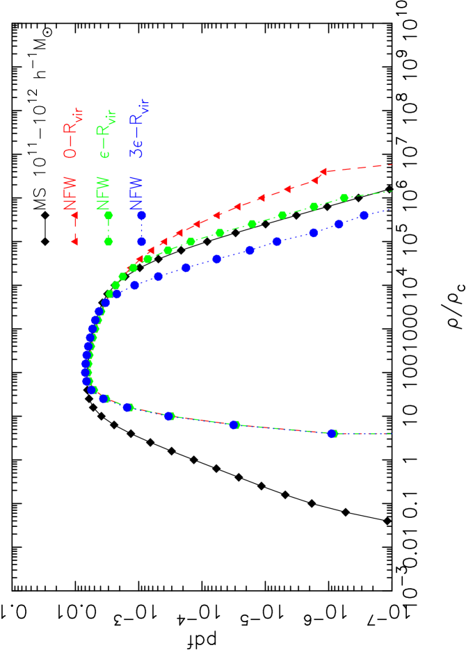
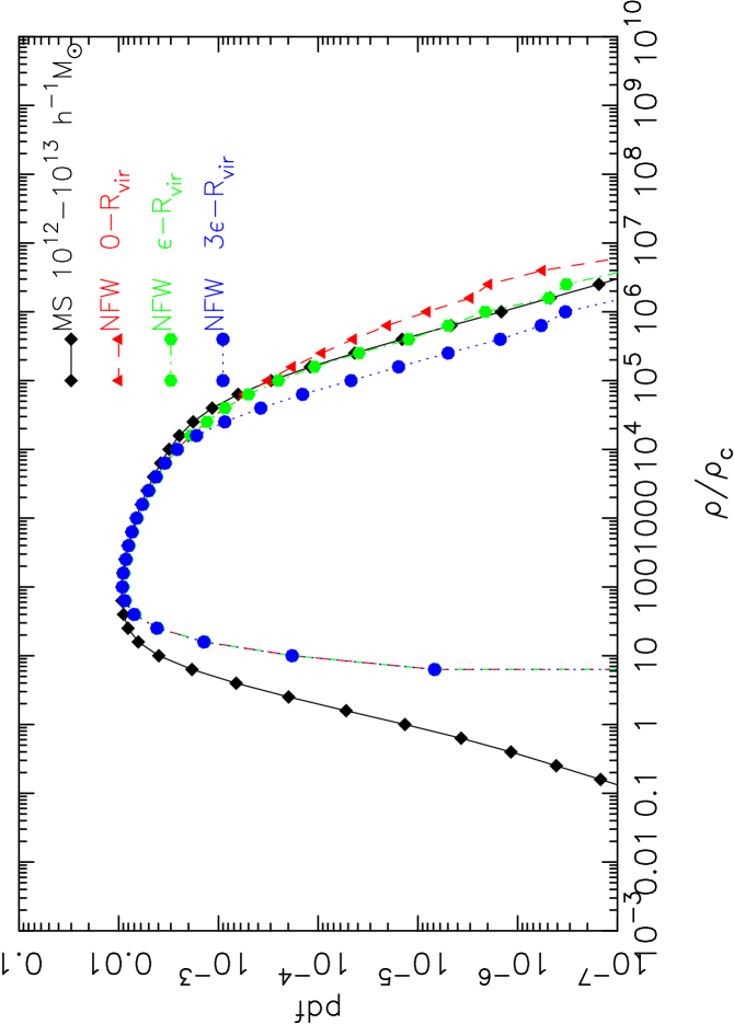
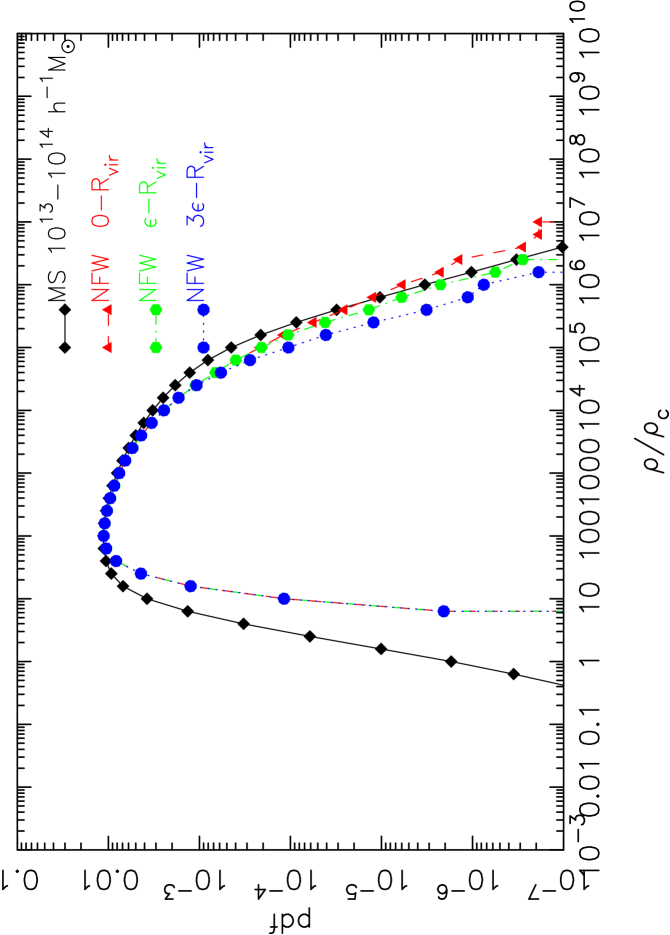
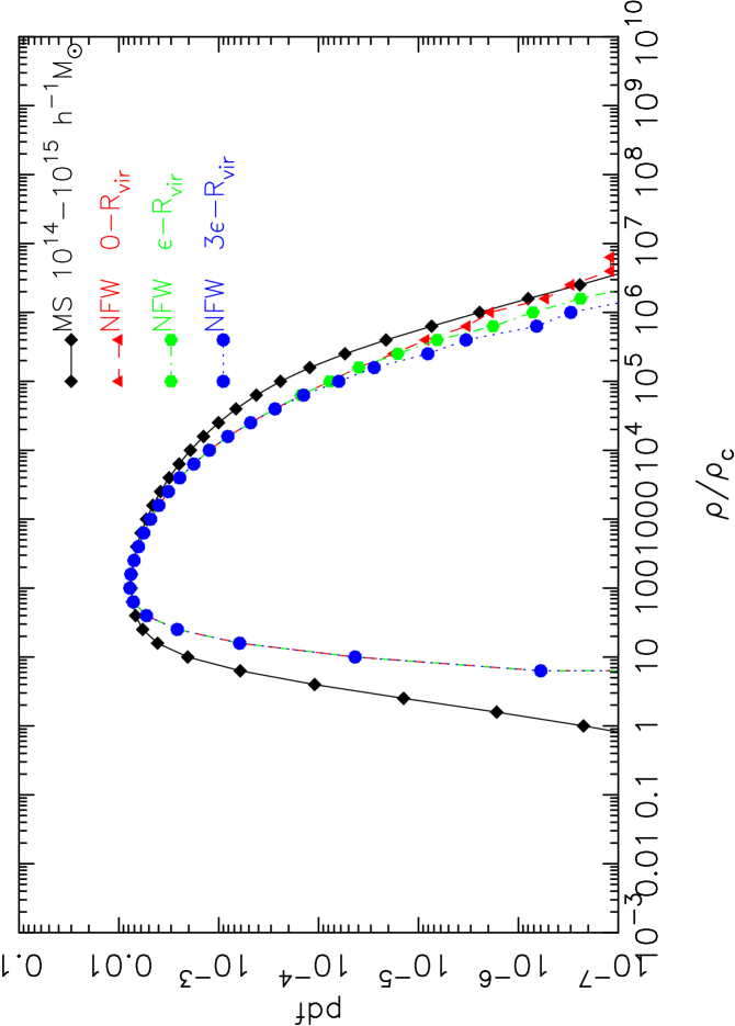
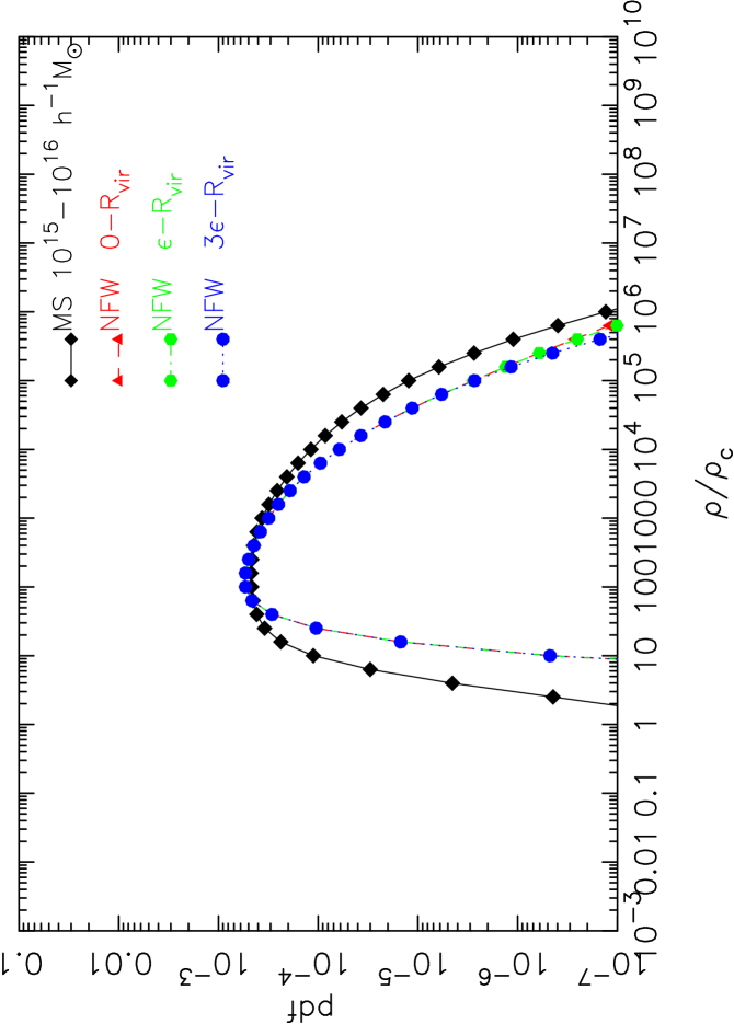
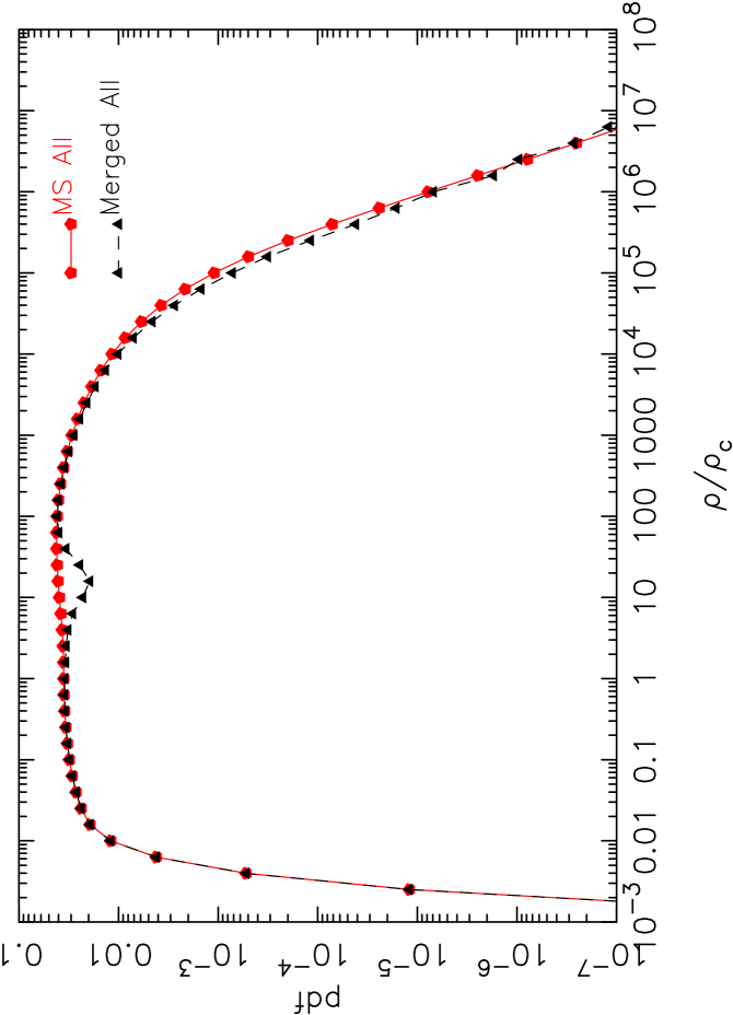
Figure 8: The top left panel shows the one-point density distribution function (black squares) of MS particles residing in halos in the mass range $10^{11}-10^{12}\,h^{-1}{\rm M}_{\sun}$. For comparison, the one-point distribution computed from Monte Carlo realizations of a NFW halo with mass $10^{12}\,h^{-1}M_{\sun}$ is scaled according to the total number of particles present in halos in the mass range $10^{11}-10^{12}\,h^{-1}M_{\sun}$. The distributions computed by restricting particles to within $r\in[0,r_{\rm vir}]$, $[1\epsilon,r_{\rm vir}]$ and $[3\epsilon,r_{\rm vir}]$ are shown in different colors and symbols. The other panels, except for the one in the bottom right, show the results for halo mass ranges $10^{12}-10^{13}$, $10^{13}-10^{14}$, $10^{14}-10^{15}$ and $10^{15}-10^{16}\,h^{-1}M_{\sun}$, respectively. Finally, the bottom right panel shows the sum of scaled distributions of NFW halos in different mass bins, and adds it to the distribution of all the non-halo particles in the simulation. The full one-point distribution of all the particles in the MS is also plotted (black triangles), for comparison. We note that while summing the distributions of Monte Carlo NFW halos over different halo mass bins we considered only particles within $r\in[1\epsilon,r_{\rm vir}]$ of the halo for the two lowest mass bins. For the rest of the bins all particles are considered.

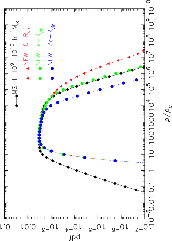
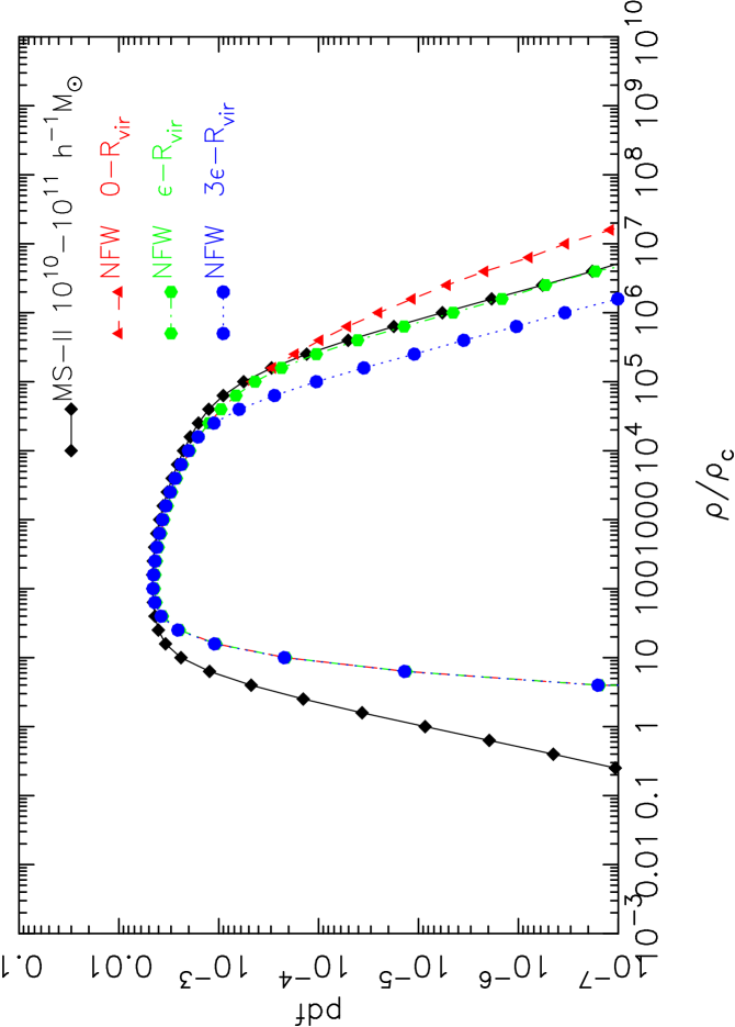
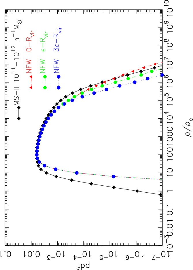
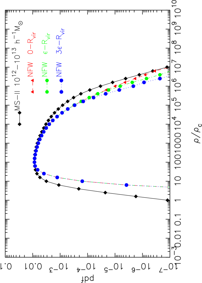
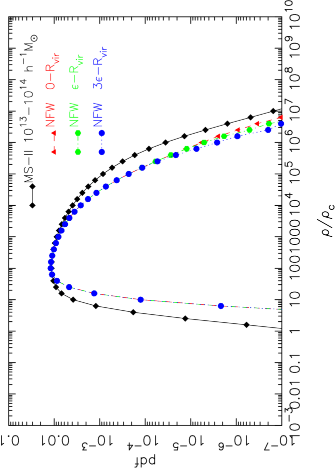
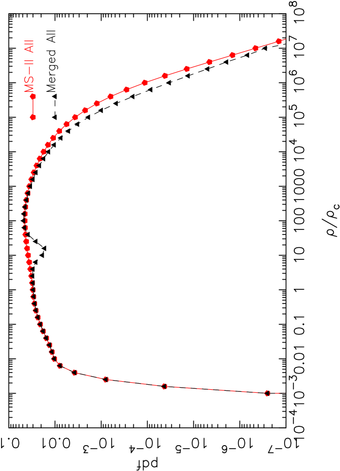
Figure 9: The same as Figure 8, but for the MS-II.

We now contrast this expected density distribution with actual measurements for the MS and MS-II when the density field is constructed with the DTFE. The probability distribution functions for all the dark matter particles at redshift $z=0$ from the MS and MS-II are shown as black curves in the two panels of Figure 4. The plots show that with the DTFE we are able to recover density values spanning about $\sim 11$ orders of magnitude, from underdense voids to the fully collapsed halos. The distribution is flat over nearly six orders of magnitude in density, and it does not exhibit any apparent linear to non-linear transition. The lower limits of the distribution functions shown in these figures have a Poisson error of $\sim 3\%$.

To isolate the contribution from collapsed halos we consider dark matter particles according to the masses of their host FoF halos. We identify the host halos by cross-matching particles IDs with FoF group IDs in the simulation. We also identify all the particles which are not part of any FoF halo with $20$ or more particles. The density distributions for each of these cases are computed separately. The results for the different components are shown together in Figure 4. It should be noted that even though the low mass halos are more concentrated compared to their high mass counterparts, the distribution systematically extends to higher density values for the higher mass halos. This is opposite to what one would naively expect. This result could be explained by the fact that the smaller mass halos are sampled with fewer particles which poorly resolve the highly concentrated cores in these halos. In addition, the effect of gravitational softening (which introduces a soft core in the halo) in N-body simulations is expected to be more severe for less massive halos as the softening length is a relatively larger fraction of their virial radii. The results for the MS-II in the right panel are quite similar, except for the fact that the overall shape of the distribution function at intermediate densities is somewhat different than that found for the MS. The distribution in this case is curvier and not quite as flat. This presumably reflects the larger fraction of particles bound in halos in the MS-II compared with the MS. It is also noticeable that at a given halo mass the density distributions extend to high densities in MS-II. Again this generally reflects the larger softening of the MS.

More detailed comparisons between MS and MS-II are shown in Figure 5. As the DTFE does not use any specific length scale for smoothing it is assured that the truncation in the tails of the distribution is not a result of a spatial resolution limit imposed by the density estimator. However, the intrinsically limited volume and mass resolution of the simulation is expected to introduce an undersampling of the tails of the distribution (Colombi, 1994; Bagla & Ray, 2005). Smaller volumes undersample rare events in both overdense and underdense regions. A similar effect is caused by lower mass resolution primarily due to its limitation in resolving lower mass halos and smaller voids. MS-II has $125$ times better mass resolution and $5$ times smaller softening length than MS enabling it to resolve the highly concentrated smaller mass subhalos. It can be seen in the top left panel of Figure 5 that the distributions in MS and MS-II are quite similar, apart from the fact that the distribution for the MS-II extends slightly more on both the low density and high density ends. The effects of finite volume and finite mass resolutions somewhat compensate each other in the MS and MS-II but the slightly extended tail of the distribution at the both end in the MS-II suggests that the combined effects of finite mass resolution and gravitational softening are more important than the effect of finite volume.

The results for the non-halo particles are shown in the top right panel. The distribution in the MS-II has lower amplitude than the MS in intermediate density ranges because of its higher mass resolution and smaller softening, which allows it to resolve more bound objects at small mass. It is also interesting to note that the high density tail of the distribution for the non-halo particles extends up to $\sim 10^{6}\,\rho_{c}$ suggesting the presence of some high density sites even outside the bound FoF halos. The distributions in different individual halo mass bins in MS and MS-II are shown in the two middle and two bottom panels. The MS-II distributions have a sharper low-density cut-off and a more extended high density tail than in the MS in all cases. Any halo of a particular mass is sampled with $125$ times more particles in MS-II than in MS. This gives MS-II better power to resolve small subhalos and the boundary of the FoF groups. Further, the softening length in MS-II is $5$ times smaller than in the MS reducing softening effects. These effects are more dominant in low mass halos and can be clearly seen as larger shifts in the lower halo mass bins. We note that we use dark matter halos identified with the FoF algorithm (Davis et al., 1985). There are also other halo finding algorithms, for example based on the spherical overdensity (SO) approach (Press & Schechter, 1974), the adaptive grouping of particles around density peaks (Eisenstein & Hut, 1998; Neyrinck et al., 2005), or the phase-space distribution of dark matter particles (Diemand et al., 2006; Maciejewski et al., 2009; Falck et al., 2012). The halo boundaries in general depend on the free parameters in the corresponding algorithms (e.g. linking length in FoF, density cut-off in SO), and the individual halos identified with different methods can sometimes vary substantially. But fortunately the mean properties of the dark matter halos agree quite well regardless of the chosen algorithm, and the differences in the halo mass functions are also quite small (Jenkins et al., 2001; Knebe et al., 2011).

In the two top panels of Figure 6, we compare our analytical halo model for the one-point distributions of the density summed over different halo mass bins against that directly obtained for the MS and MS-II. For MS and MS-II, we sum the results for $5$ and $6$ equally spaced different halo mass bins each spanning a decade in the halo mass ranges $10^{11}-10^{16}\,h^{-1}M_{\sun}$ and $10^{9}-10^{15}\,h^{-1}M_{\sun}$, respectively. We also show the ratio of the one-point distributions from the N-body data and the analytical model in the left panel of Figure 7. The excess in the observed distribution compared to the model prediction is higher in the MS-II than in the MS which is most likely related to the relative abundance of substructures. We explore this issue in detail in the remaining part of the paper. One can also clearly see a larger suppression of the high density tail of the distribution in the MS compared to the MS-II due to its larger softening length. The sharp drop in the analytical predictions in the low density regime corresponds to a truncation of the halos at their virial radii. In the bottom two panels of Figure 6, we also compare the analytical predictions for the one-point distribution function of NFW halos summed across the different halo mass bins used in the analysis, and the combined one-point distribution function of DTFE densities computed from Monte Carlo NFW halos across the same halo mass bins. The ratio of the one-point distributions from the Monte Carlo analysis and the analytic model are shown in the right panel of Figure 7. We use the same mass-concentration relation as employed for the analytic estimates. It should be noted that we are not using any fit for the halo mass function in our analytical model. The one-point distributions for the Monte Carlo NFW halos with different masses are scaled according to the total number of particles present in different halo mass bins, as directly measured in the simulations, and then summed up over all the halo mass bins. Our analytical model is based on equation (7) combined with the fact that the results for each halo mass bin are scaled by exactly the same amount as their Monte Carlo counterparts. The results for different halo mass bins are then summed up. We see that the analytical one-point distribution function is quite well described by the results from Monte Carlo simulations, apart from the fact that the analytical predictions show a sharp drop in the distribution function due to the truncation of all NFW halos at $r_{200}$. The DTFE densities do not show this sharp drop due to the Poisson sampling of the halos. The slightly more extended high density tail seen in the MS-II comes from its ability to incorporate lower mass halos which are more concentrated. Thus, the DTFE traces the analytical one-point distribution function of the densities quite well, and the amount of excess (substructure) and the shape of the high density tail of the distribution in the N-body simulations are governed by the mass resolution, gravitational softening and simulated volume.

We have also modeled the one-point distributions for different mass bins in the N-body simulations with ideal spherical NFW halos of similar masses. For this we generate $10^{4}$ , $10^{3}$, $10^{2}$ , $10$ and $1$ Monte Carlo realizations of NFW halos with masses $10^{12}\,h^{-1}\,M_{\odot}$, $10^{13}\,h^{-1}\,M_{\odot}$, $10^{14}\,h^{-1}\,M_{\odot}$, $10^{15}\,h^{-1}\,M_{\odot}$ and $10^{16}\,h^{-1}\,M_{\odot}$, respectively. We use the mass-concentration relation given by Neto et al. (2007) and the particle mass $8.61\times 10^{8}\,h^{-1}\,M_{\odot}$ of the MS. The concentration of halos depends very weakly on mass, and for simplicity we assume that the concentration does not change significantly within each of the narrow halo mass ranges. Different numbers of halos for the different mass ranges are constructed to account for the effects of discreteness i.e. to incorporate the fact that a $10^{n_{1}}\,h^{-1}\,M_{\odot}$ halo is resolved with $10^{{n_{1}}/{n_{2}}}$ times more particles than a $10^{n_{2}}\,h^{-1}\,M_{\odot}$ halo for any given values of $n_{1}$ and $n_{2}$ (where $n_{1}>n_{2}$). We use all the density estimates from $10^{{n_{1}}/{n_{2}}}$ simulated NFW halos with mass $10^{n_{2}}\,h^{-1}\,M_{\odot}$ to compute their one-point distribution, ensuring that the same number of density estimates are used to determine the one-point distribution of density for NFW halos with different masses. We followed the same approach for the MS-II as well, except that here we can go down another two decades in halo mass. We use the same mass-concentration relation for the MS-II, extrapolated to lower halo masses as needed.

We compute in this way the one-point distribution of Monte Carlo NFW halos with different masses, and then scale them according to the total number of particles present in different halo mass bins as directly measured in the MS, in order to compare the theoretical predictions of this simple halo model with the measurements directly obtained from the MS (Figure 8). It should be noted that we have not used the halo mass function to model the one-point distribution here. Instead, we have used the total number of particles in a halo mass bin to predict the expected one-point distribution from halos in that bin. The results of this comparison for the MS and the MS-II are shown in Figures 8 and 9, respectively.

We find that the one-point distribution in each mass bin is reproduced nicely at intermediate densities when the results for the Monte Carlo NFW halos in that mass bin are scaled according to the total number of particles found in the N-body simulation in the same mass bin (Figures 8 and 9). The low density part of the distribution in each mass bin is however missed by the theoretical toy model. This is to be expected as we are only considering the particles within the virial radii of the spherical mock NFW halos, whereas in reality the FoF halos in N-body simulations extend beyond their virial radii and generally have quite irregular shapes near their edges. At higher densities, the lower mass bins show higher values of the PDF for the theoretical one-point distribution compared with the N-body simulations. This is because the mock NFW halos do not involve any softening whereas a gravitational softening is present in the N-body simulations from where the FoF halos are identified. In order to explicitly check for the impact of the softening length ($\epsilon$) in N-body simulations we have made an experiment where we prevented that particles in the mock halos are placed within $1\epsilon$ from their centers when computing the one-point distribution for all NFW halos in each mass bin. Interestingly, when we limit the particles to the radii outside of the softening range, the high density tail is nicely consistent between the N-body simulations and the mock halos. It thus seems clear that softening primarily affects the high density tail of the one-point distribution by suppressing the highest density values. This simple explanation does not work as well for the highest halo mass bins, presumably because their structure is less strongly affected by the softening and they feature much more halo substructure.

It is interesting to note that the one-point distribution in the higher halo mass bins shows an excess over the theoretical prediction. The fractions of particles in each halo mass bin which account for this excess are different and increase with increasing halo masses. Specific numbers for our measurements are reported in Table 2. In a smooth NFW halo, there are no substructures whereas the halos formed in N-body simulations host numerous small subhalos that typically account for a few percent up to $\sim 15\%$ of the mass. The excess we find in the one-point distributions is most likely the direct consequence of the presence of substructures in the massive dark matter halos formed in N-body simulations. The excess accounts for up to $\sim 8-10\%$ of the total particles in the highest halo mass bin, consistent with typical substructure mass fractions. The excess decreases with halo mass and is completely absent or almost negligible in the lowest mass bins. Again, the decrease in the amount of substructures with decreasing halo mass is consistent with previous findings (Gao et al., 2004) and with expected numerical resolution limitations. Further, it is to be noted that the MS-II shows a higher substructure abundance compared to the MS in each halo mass bin. This is related both to the higher mass resolution and to the smaller softening length in the MS II which enables it to resolve lower mass subhalos.

The effect of substructures on the one-point distribution is shown explicitly in Figure 10, which focuses on a well resolved halo from the MS-II. The substructures in the MS-II halo are here identified with the SUBFIND algorithm (Springel et al., 2001) and are available from the MS-II database. We identified all the particles within $1.5\,r_{\rm vir}$ around the center of that halo and computed the one-point distribution of the density. We then removed all the substructure particles within that radius and computed the distribution function again. The results are compared in Figure 10, which clearly highlights the excess due to the presence of substructures in the halo. The substructures constitute $\sim 6.5\%$ of the total particles in this halo within our chosen radius, and this fraction is consistent with the values listed in Table 2.

One should also keep in mind that the dark matter halos in simulations are not exactly spherical. Rather their shapes resemble in general triaxial ellipsoids with a preference for prolate configurations (Dubinski & Carlberg, 1991; Cole & Lacey, 1996; Jing & Suto, 2002; Vogelsberger et al., 2009). The shapes of the majority of the halos forming in N-body simulations are characterized by a mean axis ratio of about $1:0.74:0.64$ (Kasun & Evrard, 2005; Bailin & Steinmetz, 2005; Allgood et al., 2006). Fitting a NFW profile to such halos inevitably involves spherical averaging. The spherical averaging of a triaxial halo will introduce systematic differences in the density estimates in different parts of the halo. Some parts of the halo have in reality densities which are larger/smaller than the spherically averaged densities we try to reproduce in our mock models. This deviation in the densities could be quite high depending on the triaxiality of the dark matter halos and it is important to investigate if the excess in the observed one-point distribution of density is related to this issue. In order to test this we simulated a triaxial NFW halo of mass $M_{200}=10^{14}\,h^{-1}\,M_{\odot}$ with axis ratios $a:b:c=1.5:0.888:0.75$. To mimic the effect of sphericalization we randomize the azimuthal co-ordinates ($\theta$, $\phi$) of all the particles in the halo. The one-point distribution function of the triaxial halo before and after sphericalization are compared in Figure 11 where we can see that this effect does not make a significant change in the one-point distribution function of density despite our choice of a deliberately extreme (yet still possible) axis ratio. This result suggests that the observed excesses in the one-point distributions (Figures 8 and 9) are a direct outcome of the substructures present in the dark matter halos, and that the halo shape plays only a very subdominant role.

As an aside, we note that the dependence of substructure abundance on mass resolution has important implications for predictions of the expected extragalactic gamma ray background hypothetically caused by the self-annihilation of dark matter particles in dark matter halos. The rate of WIMP annihilation and hence the intensity of the annihilation radiation in a dark matter halo is proportional to the volume integral of the square of the dark-matter density. The existence of lumps or subhalos in dark matter halos is expected to enhance the annihilation rate by a significant boost factor (Bergström et al., 1999; Stoehr et al., 2003; Koushiappas et al., 2004; Pieri et al., 2005; Kuhlen et al., 2008; Springel et al., 2008; Kuhlen et al., 2009; Kamionkowski et al., 2010). The smallest subhalos are the densest sites in the halo and the predicted boost factor depends significantly on how well these subhalos are resolved in the N-body simulations. Given that halos in the MS-II host more resolved substructures than the MS indicates that the theoretical prediction of the intensity of annihilation signal from any simulated dark matter halo depends on the resolving power imposed by the softening length and by the finite mass resolution. One has to correct for this by extrapolating the relations between substructure abundance and mass resolution (at a fixed softening length) to lower particle masses in order to make a prediction about the signal expected in reality.

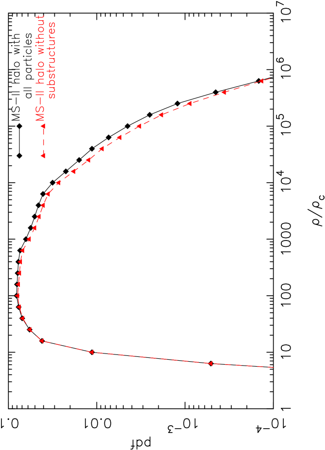
Figure 10: The one point distribution of density for a halo from the MS-II for all the particles residing within $1.5\,r_{200}$ around the halo centre. For comparison, the red dashed line shows the one-point distribution of the same halo after all its substructures within $1.5\,r_{200}$ has been removed. The virial radii of this halo is $0.60\,h^{-1}\,{\rm Mpc}$, and a total of $8079161$ particles reside within $1.5\,r_{200}$, out of which $528753$ ($\sim 6.5\%$) are subhalo members.

We combine the results of our Monte Carlo simulations of NFW halos in different mass bins, and add also the one-point distribution of the non-halo particles found in simulations to obtain a halo model for the full one-point distributions in the MS and MS-II. The results are shown in the bottom right panel of Figures 8 and 9. The dip in the middle of the distributions results from the truncated spherical boundaries of the idealized NFW halos, which does not take into account the fact that the real halos in simulations are far more irregular at their boundaries and extend to lower densities as well. At higher densities, there are nevertheless also differences between the direct results of the N-body simulations and the Monte Carlo model. Clearly, larger differences are seen in the case of the MS-II compared with the MS, an effect that we attribute to the higher abundance of substructures in the MS-II.

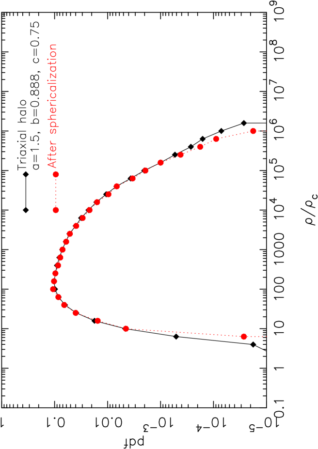
Figure 11: One-point density distribution function of a Monte Carlo realization of a triaxial NFW halo (black) of mass $M_{200}=10^{14}\,h^{-1}M_{\sun}$, represented with particle mass $8.61\times 10^{8}\,h^{-1}M_{\sun}$. The density distribution function of the same halo after sphericalization is shown in red. To avoid any boundary effects only the particles inside $r_{200}$ are used in both cases.

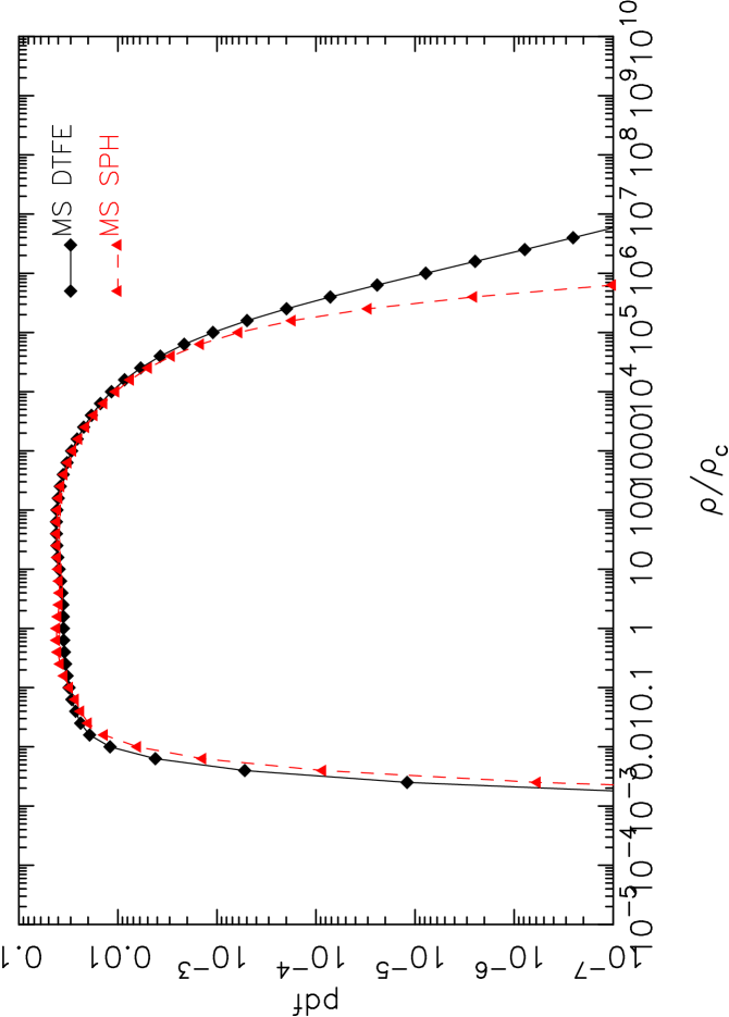
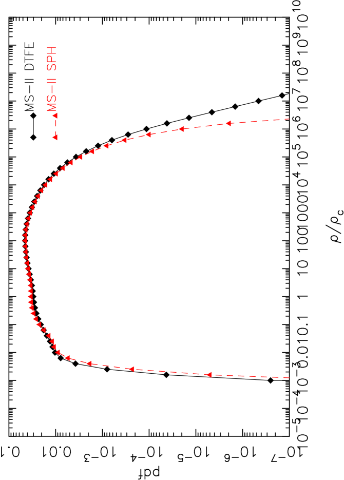
Figure 12: Comparison of the density distributions measured with DTFE and SPH smoothing. The top and bottom panels show results for the MS and the MS-II, respectively.

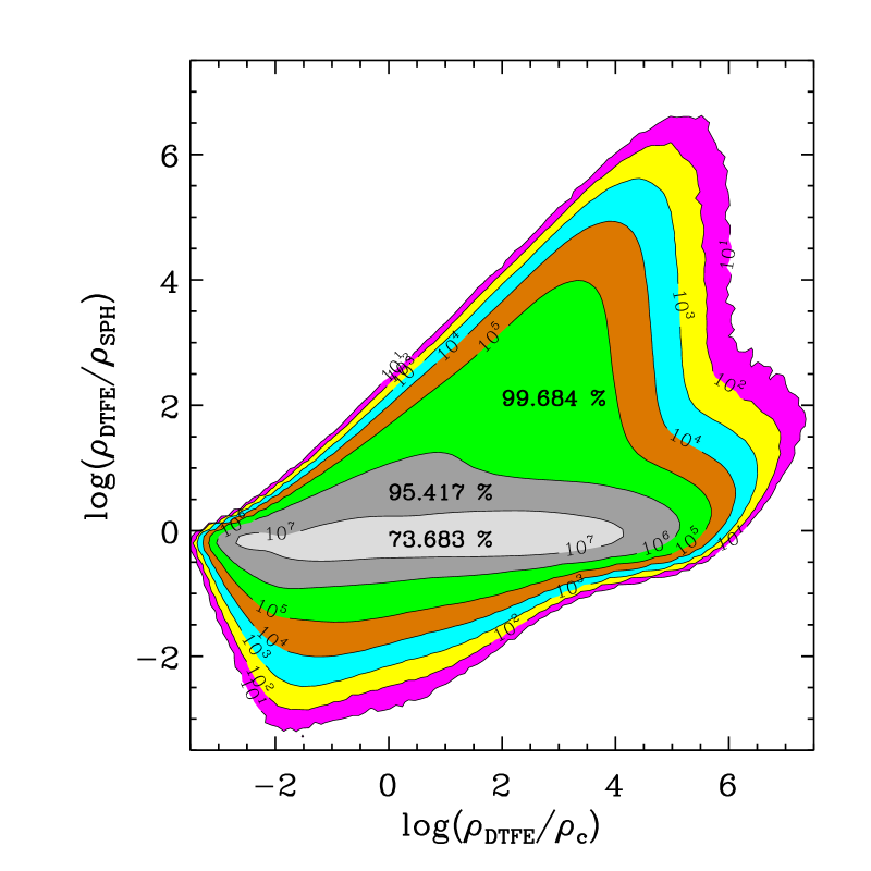
Figure 13: Two-dimensional histogram of the ratio of DTFE to SPH density estimated for the MS-II, as a function of the DTFE density. A total of $100\times 100$ pixels are used to estimate the histogram. Different contours correspond to the pixels with a count equal to the numbers used for labeling the respective contours. Different coloured regions mark the pixels with counts intermediate to their bounding contours. The numbers shown inside the coloured regions give the total cumulative counts in all the pixels contained inside the outer contours of the corresponding regions. This plot clearly shows the systematic overestimate and underestimate of densities by SPH over DTFE at low and high densities, respectively.

Finally, we compare the distribution of DTFE and SPH densities from the MS and MS-II in Figure 12 to check how the choice of density estimator influences the tails of the distribution. The smoothing lengths in SPH are chosen such that the sum involves $32$ nearest neighbours. This figure shows that for the lowest density regions or voids the DTFE and SPH smoothing give very similar results. At very low densities, the slightly higher values found in the DTFE distribution come probably from a more accurate representation of void boundaries than in SPH. Similarly, the extended kernel of SPH smoothes out high density regions like filaments or halo centers leading to an underestimate of the PDF in such regions. In both the MS and MS-II there is a small bump in the density range $0.1-5\rho_{c}$ displaying an excess of the SPH density estimate as compared to the DTFE density measurement.

In Figure 13, we show how the DTFE and SPH density estimates compare with each other at different densities in the MS-II. It can be clearly seen that for most of the particles, DTFE and SPH give comparable results, while residual systematic differences show up as oppositely skewed tails at high and low densities. These systematic differences in low and high density regions account for the differences in the SPH and DTFE density distributions. A detail comparison between DTFE and SPH is given in Pelupessy et al. (2003) and our findings are consistent with theirs. Recently, Abel et al. (2012) pointed out that even the VTFE underestimates the densities in regions around filaments and sheets, as compared to a novel technique that more accurately represents dark phase-space sheets. So besides factors like mass resolution, gravitational softening and simulated volume, the choice of density estimator plays a crucial role in shaping the tails of the density distribution.

4 Conclusions

The present analysis shows that the part of the one-point distribution function represented by collapsed halos can be quite well described by a simple superposition of a set of NFW halos over different mass ranges. However, the one-point distribution functions in N-body simulations also show a prominent hump when individual halo mass bins are considered, especially for the more massive halos. This excess with respect to the distribution obtained for smooth NFW halos originates in the substructures present in the massive dark matter halos. The amount of resolved substructures depends on the mass of the halo, and especially on the finite mass resolution of the N-body simulation. Further, the gravitational softening suppresses the high density tail of the one-point distribution in halos, introducing a soft core which is more noticeable in smaller mass halos. Both of these effects imply that the high-density tail is still underestimated both in the direct N-body simulations and the analytical halo model.

We find that finite simulation volume, finite mass resolution, gravitational softening as well as the method for estimating the density field all influence the tails of the measured one-point density distribution. We note that this distribution function is a particularly important simulation prediction, as it, for example, determines the intensity of the WIMP annihilation signal from a representative volume, which sensitively depends on the ability to resolve the abundant yet dense small-mass structures. Our analysis with the DTFE in the MS and MS-II suggests that the effect of finite mass resolution and gravitational softening are the primary limitations rather than a finite simulation volume. Also, it is worthwhile to employ the DTFE techniques instead of simpler schemes for density reconstruction such as SPH-like smoothing, due to its sharper resolving power.

References

- Abel et al. (2012) Abel T., Hahn O., Kaehler R., 2012, MNRAS, 427, 61
- Allgood et al. (2006) Allgood B., Flores R. A., Primack J. R., et al., 2006, MNRAS, 367, 1781
- Aragón-Calvo et al. (2007) Aragón-Calvo M. A., Jones B. J. T., van de Weygaert R., van der Hulst J. M., 2007, A&A, 474, 315
- Ascasibar & Binney (2005) Ascasibar Y., Binney J., 2005, MNRAS, 356, 872
- Bagla & Ray (2005) Bagla J. S., Ray S., 2005, MNRAS, 358, 1076
- Bailin & Steinmetz (2005) Bailin J., Steinmetz M., 2005, ApJ, 627, 647
- Bardeen et al. (1986) Bardeen J. M., Bond J. R., Kaiser N., Szalay A. S., 1986, ApJ, 304, 15
- Bergström et al. (1999) Bergström L., Edsjö J., Gondolo P., Ullio P., 1999, Phys. Rev. D, 59, 4, 043506
- Boylan-Kolchin et al. (2009) Boylan-Kolchin M., Springel V., White S. D. M., Jenkins A., Lemson G., 2009, MNRAS, 398, 1150
- Cole & Lacey (1996) Cole S., Lacey C., 1996, MNRAS, 281, 716
- Coles & Jones (1991) Coles P., Jones B., 1991, MNRAS, 248, 1
- Colless et al. (2001) Colless M., Dalton G., Maddox S., et al., 2001, MNRAS, 328, 1039
- Colombi (1994) Colombi S., 1994, ApJ, 435, 536
- Cooray & Sheth (2002) Cooray A., Sheth R., 2002, Phys. Rep., 372, 1
- Davis et al. (1985) Davis M., Efstathiou G., Frenk C. S., White S. D. M., 1985, ApJ, 292, 371
- Delaunay (1934) Delaunay B. N., 1934, Sur la sphere vide: Izv. Akad. Nauk SSSR, Otdel. Mat. Est. Nauk, 7, 793
- Diemand et al. (2006) Diemand J., Kuhlen M., Madau P., 2006, ApJ, 649, 1
- Dubinski & Carlberg (1991) Dubinski J., Carlberg R. G., 1991, ApJ, 378, 496
- Eisenstein & Hut (1998) Eisenstein D. J., Hut P., 1998, ApJ, 498, 137
- Falck et al. (2012) Falck B. L., Neyrinck M. C., Szalay A. S., 2012, ApJ, 754, 126
- Gao et al. (2004) Gao L., White S. D. M., Jenkins A., Stoehr F., Springel V., 2004, MNRAS, 355, 819
- Hockney & Eastwood (1981) Hockney R. W., Eastwood J. W., 1981, Computer Simulation Using Particles, McGraw-Hill, New York
- Jenkins et al. (2001) Jenkins A., Frenk C. S., White S. D. M., et al., 2001, MNRAS, 321, 372
- Jing (2000) Jing Y. P., 2000, ApJ, 535, 30
- Jing & Suto (2002) Jing Y. P., Suto Y., 2002, ApJ, 574, 538
- Kamionkowski et al. (2010) Kamionkowski M., Koushiappas S. M., Kuhlen M., 2010, Phys. Rev. D, 81, 4, 043532
- Kasun & Evrard (2005) Kasun S. F., Evrard A. E., 2005, ApJ, 629, 781
- Kayo et al. (2001) Kayo I., Taruya A., Suto Y., 2001, ApJ, 561, 22
- Kiang (1966) Kiang T., 1966, ZAp, 64, 433
- Knebe et al. (2011) Knebe A., Knollmann S. R., Muldrew S. I., et al., 2011, MNRAS, 415, 2293
- Kofman et al. (1994) Kofman L., Bertschinger E., Gelb J. M., Nusser A., Dekel A., 1994, ApJ, 420, 44
- Koushiappas et al. (2004) Koushiappas S. M., Zentner A. R., Walker T. P., 2004, Phys. Rev. D, 69, 4, 043501
- Kuhlen et al. (2008) Kuhlen M., Diemand J., Madau P., 2008, ApJ, 686, 262
- Kuhlen et al. (2009) Kuhlen M., Madau P., Silk J., 2009, Science, 325, 970
- Maciejewski et al. (2009) Maciejewski M., Colombi S., Springel V., Alard C., Bouchet F. R., 2009, MNRAS, 396, 1329
- Monaghan (1992) Monaghan J. J., 1992, ARA&A, 30, 543
- Navarro et al. (1996) Navarro J. F., Frenk C. S., White S. D. M., 1996, ApJ, 462, 563
- Navarro et al. (1997) Navarro J. F., Frenk C. S., White S. D. M., 1997, ApJ, 490, 493
- Neto et al. (2007) Neto A. F., Gao L., Bett P., et al., 2007, MNRAS, 381, 1450
- Neyrinck et al. (2005) Neyrinck M. C., Gnedin N. Y., Hamilton A. J. S., 2005, MNRAS, 356, 1222
- Okabe et al. (2000) Okabe A., Boots B., Sugihara K., Nok Chiu S., 2000, Spatial Tessellations, Concepts and Applications of Voronoi Diagrams, John Wiley & Sons Ltd, Chichester
- Pelupessy et al. (2003) Pelupessy F. I., Schaap W. E., van de Weygaert R., 2003, A&A, 403, 389
- Pieri et al. (2005) Pieri L., Branchini E., Hofmann S., 2005, Physical Review Letters, 95, 21, 211301
- Platen et al. (2011) Platen E., van de Weygaert R., Jones B. J. T., Vegter G., Calvo M. A. A., 2011, MNRAS, 416, 2494
- Press & Schechter (1974) Press W. H., Schechter P., 1974, ApJ, 187, 425
- Schaap (2007) Schaap W. E., 2007, DTFE: the Delaunay Tessellation Field Estimator, Ph.D. thesis, Kapteyn Astronomical Institute
- Schaap & van de Weygaert (2000) Schaap W. E., van de Weygaert R., 2000, A&A, 363, L29
- Silverman (1986) Silverman B. W., 1986, Density estimation for statistics and data analysis, Chapman and Hall, London
- Springel (2010) Springel V., 2010, MNRAS, 401, 791
- Springel et al. (2008) Springel V., White S. D. M., Frenk C. S., et al., 2008, Nature, 456, 73
- Springel et al. (2005) Springel V., White S. D. M., Jenkins A., et al., 2005, Nature, 435, 629
- Springel et al. (2001) Springel V., White S. D. M., Tormen G., Kauffmann G., 2001, MNRAS, 328, 726
- Stoehr et al. (2003) Stoehr F., White S. D. M., Springel V., Tormen G., Yoshida N., 2003, MNRAS, 345, 1313
- Stoughton et al. (2002) Stoughton C., Lupton R. H., Bernardi M., et al., 2002, AJ, 123, 485
- Taruya et al. (2003) Taruya A., Hamana T., Kayo I., 2003, MNRAS, 339, 495
- van de Weygaert (1994) van de Weygaert R., 1994, A&A, 283, 361
- van de Weygaert (2007) van de Weygaert R., 2007, ArXiv e-prints
- Vogelsberger et al. (2009) Vogelsberger M., Helmi A., Springel V., et al., 2009, MNRAS, 395, 797
- White & Rees (1978) White S. D. M., Rees M. J., 1978, MNRAS, 183, 341
- Zhang et al. (2010) Zhang Y., Springel V., Yang X., 2010, ApJ, 722, 812