A fast multigrid-based electromagnetic eigensolver for curved metal boundaries on the Yee mesh

Abstract

For embedded boundary electromagnetics using the Dey–Mittra [1] algorithm, a special grad-div matrix constructed in this work allows use of multigrid methods for efficient inversion of Maxwell’s curl-curl matrix. Efficient curl-curl inversions are demonstrated within a shift-and-invert Krylov-subspace eigensolver (open-sourced at https://github.com/bauerca/maxwell) on the spherical cavity and the 9-cell TESLA superconducting accelerator cavity. The accuracy of the Dey–Mittra algorithm is also examined: frequencies converge with second-order error, and surface fields are found to converge with nearly second-order error. In agreement with previous work [2], neglecting some boundary-cut cell faces (as is required in the time domain for numerical stability) reduces frequency convergence to first-order and surface-field convergence to zeroth-order (i.e. surface fields do not converge). Additionally and importantly, neglecting faces can reduce accuracy by an order of magnitude at low resolutions.

1 Introduction

The Dey-Mittra electromagnetics algorithm simulates smooth curved perfectly-conducting boundaries using the Yee finite-difference technique [3, 1]. The algorithm is often called a cut-cell or embedded-boundary technique since the mesh does not conform to the geometry of the conducting boundary (grid cells, faces, and edges are “cut” by boundaries). In the time-domain, the Courant-Friedrichs-Lewy (CFL) condition reduces the accuracy of the Dey–Mittra algorithm by requiring the neglecting of some cut faces. More precisely, the CFL condition states that the maximum stable timestep is limited by the maximum eigenvalue (of the discretized curl-curl matrix) and, in the Dey–Mittra algorithm, the maximum eigenvalue can be inflated greatly by faces barely cut by a boundary. A trade-off between accuracy and wall-clock simulation time ensues; if fewer neglected faces are desired (greater accuracy), the time-step must be reduced [1, 2]. In this paper, we consider the Dey–Mittra algorithm in the frequency-domain, where the CFL condition does not apply and the full accuracy of the method can be used.

We begin by reviewing the two important aspects of the problem: (1) the Dey–Mittra algorithm and (2) eigensolving Maxwell’s equations as discretized on the Yee mesh (ultimately, this leads to the question: how does one invert the curl-curl operator? Fortunately, this is well-studied [4, 5, 6, 7, 8, 9]). The advance of this paper is described in Section 5, and amounts to a transformation of the discretized Dey–Mittra curl-curl operator that allows efficient inversion by multigrid techniques [10]. Proof of performance is given in the numerical results, where our eigensolver attacks the spherical resonant cavity and the 9-cell TESLA superconducting accelerator cavity. The code used throughout this paper is open-sourced, and can be found at https://github.com/bauerca/maxwell.

2 The Dey–Mittra algorithm

Electromagnetic cavity eigenmodes are solutions to Maxwell’s wave equation subject to perfectly conducting boundary conditions; a magnetic eigenmode satisfies

$$\nabla\times\nabla\times{\bf B} =k^{2}{\bf B}\quad\text{in $\Omega$}$$ (1)

$$\mathbf{n}\cdot\mathbf{B} =0\quad\text{on $\partial\Omega$}$$ (2)

where $\Omega$ is the cavity interior, $\partial\Omega$ is the perfectly conducting boundary, $\mathbf{n}$ is the normal to the boundary, and $k=\omega/c$, where $\omega$ is the resonant angular frequency and $c$ is the speed of light. We discretize Maxwell’s equations with the finite-difference Yee algorithm [3], labeling the grid electric and magnetic field components as $e_{\alpha|ijk}$ and $b_{\alpha|ijk}$, respectively, where $\alpha$ is one of $x$, $y$, or $z$ and $i$, $j$, and $k$ are integer grid cell indices. Figure 1 shows the spatially staggered component layout of the Yee scheme which ensures the first-order accuracy (second-order error) of the discretized curl operators. In matrix-vector form, where $\mathbf{b}$ ($\mathbf{e}$) is the vector of all $b_{\alpha|ijk}$ ($e_{\alpha|ijk}$) components, the discretized version of Eq. (1) in vacuum is written [11, 12]

$${\rm CC^{T}}{\bf b}=k^{2}{\bf b}.$$ (3)

The Yee layout guarantees that the curl of the electric field is the transpose of the curl of the magnetic field, resulting in the symmetric matrix of Eq. 3 (the curl-curl matrix is also positive semi-definite, i.e. $k^{2}\geq 0$).

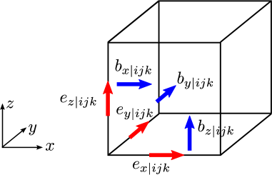
Figure 1: Color online. Yee grid cell $ijk$. Electric (Magnetic) field components are centered on edges (faces).

The Dey-Mittra algorithm is a modification of the Yee algorithm which simulates curved perfectly conducting boundaries in 3D with second-order error [1, 2]. The algorithm is based on the finite integral interpretation of the Yee algorithm [13, 14] where, for example, the Yee Faraday update for $b_{x|ijk}$ (in the frequency domain) is written as

$$-i\omega b_{x|ijk}=\frac{1}{a_{x|ijk}}\left(l_{y|ijk}e_{y|ijk}-l_{y|ijk+1}e_{y|ijk+1}+l_{z|ij+1k}e_{z|ij+1k}-l_{z|ijk}e_{z|ijk}\right),$$ (4)

which is a representation of Faraday’s Law in integral form: $-i\omega\int\mathbf{B}\cdot d\mathbf{a}=\oint\mathbf{E}\cdot d\mathbf{l}$. In the above, $l_{\alpha|ijk}$ is the length of the edge of the Yee grid cell on which the component, $e_{\alpha|ijk}$, is centered (see Fig. 1). Similarly, $a_{\alpha|ijk}$ is the area of the cell face on which the component, $b_{\alpha|ijk}$, is centered. In vacuum, $l_{x|ijk}=\Delta x$, $l_{y|ijk}=\Delta y$, and $a_{x|ijk}=\Delta y\Delta z$ such that Eq. (4) reduces to the usual Yee finite difference expression.

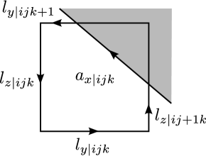
Figure 2: An example of a cut face. The shaded region is conductor. In the Dey–Mittra method, the loop integral for Faraday’s update is performed along the arrow-indicated contour. Because tangential electric fields are zero at perfectly-conducting boundaries, the line integral along the surface is skipped.

When a face, $a_{\alpha|ijk}$ is intersected by a perfectly conducting boundary, the Dey–Mittra algorithm takes $l_{\alpha|ijk}$ and $a_{\alpha|ijk}$ to be the portion of the length and area, respectively, outside the conductor (see Fig. 2). This is a physically meaningful representation of Faraday’s Law in integral form since the electric field tangent to conducting boundaries vanishes. In matrix-vector form, the Dey–Mittra algorithm changes Eq. (3) to

$${\rm A^{-1}CLC^{T}}{\bf b}=k^{2}{\bf b}$$ (5)

where $\rm A$ is a diagonal matrix of cell face fractions (e.g., ${\rm A}_{(x|ijk)(x|ijk)}=a_{x|ijk}/\Delta y\Delta z$) and $\rm L$ is a diagonal matrix of cell edge fractions (e.g., ${\rm L}_{(x|ijk)(x|ijk)}=l_{x|ijk}/\Delta x$).

Vanishing area fractions lead to very large elements in the inverse area fraction matrix ${\rm A}^{-1}$ which can then inflate the maximum eigenvalue of the Dey–Mittra curl-curl matrix (relative to the vacuum Yee algorithm). For this reason, as summarized in the next section, the Dey–Mittra algorithm cannot be used to its full potential in the time-domain. Following the next section, the rest of this paper considers the frequency-domain, where this restriction is no longer an issue.

3 Dey–Mittra: weakened for the time-domain

To use Dey–Mittra in the time-domain, one must neglect certain cut faces with small area fractions, thus reducing the accuracy of the algorithm. In the standard Yee leap-frog time-stepping scheme, the Courant-Friedrichs-Lewy (CFL) condition states that the maximum eigenvalue of Eq. 5 limits the maximum stable timestep. In 3D vacuum, the CFL condition on the timestep $\Delta t$ is

$$\Delta t<\Delta t_{\rm CFL}\equiv\frac{1}{c\sqrt{\frac{1}{\Delta x^{2}}+\frac{1}{\Delta y^{2}}+\frac{1}{\Delta z^{2}}}}.$$ (6)

In the Dey–Mittra algorithm, small area fractions amplify elements of the matrix ${\rm A}^{-1}$. For some cuts, the edge lengths in the numerator of Eq. 4 do not compensate, and the largest eigenvalue of the Dey–Mittra wave equation (Eq. 5) can be larger than that of the vacuum Yee wave equation (Eq. 3). Therefore, the Dey–Mittra time-domain algorithm can require a much reduced timestep as compared to $\Delta t_{\rm CFL}$ [2].

Alternatives to and modifications of the Dey–Mittra algorithm have been suggested that try to avoid the unfavorable CFL condition. The algorithm of [15] is complicated, but retains the second-order convergence of Dey-Mittra without reduction in timestep (compared to $\Delta t_{\rm CFL}$) by expanding the stencil for components with small area fractions (effectively averaging/enlarging the curl of $\bf E$ update for that component). Another simple modification of Dey–Mittra retains the small boundary stencil and the vacuum CFL timestep, but at the expense of second-order convergence [16]; however, it achieves low absolute frequency errors in the numerical tests. A different approach corrects for the errors induced by stairstepping the boundary [17, 18]; however, to ensure energy conservation (and thus, long-time numerical stability), linear solves are required to find the operator coefficients on the boundary. This has been demonstrated only in 2D [18].

With Dey–Mittra, the usual approach to avoid prohibitively small timesteps is to neglect faces with small area fractions, resulting in a pointy perturbation of the original conducting boundary. Unfortunately, neglected faces reduce the frequency convergence of the Dey–Mittra algorithm to first-order [2]. The alternatives mentioned in the previous paragraph perform well compared to the Dey–Mittra algorithm with neglected faces.

Our new eigensolver allows the keeping of all cut faces without degradation of the solution time (that is, given a simulation and resolution, solution times are the same whether faces are neglected or not). Given this ease, the effects of neglecting faces are probed in more detail in this paper as compared to the results of Ref. [2]. Namely, in addition to confirming the first-order frequency convergence induced by neglecting faces, we also highlight the stagnation of field convergence for fields on the surface of the conducting boundary.

The technique used to neglect small face fractions in Ref. [2] analyzes the Gershgorin Circle for every boundary face to minimize the number ignored. For simplicity, we have implemented a less sophisticated face-neglecting technique. We define a minimum area fraction, $a_{\rm min}$; magnetic field components associated with area fractions less than $a_{\rm min}$ are set to zero (i.e. the face is neglected). Electric field components on edges of the neglected face are also set to zero.

4 Eigensolving the Yee vacuum wave equation

Simulations of interest (especially in accelerator component design) routinely require millions of grid cells to achieve the desired accuracy. The curl-curl matrix in Eq. 3 or 5 therefore has millions of rows and cannot be fully diagonalized. Iterative eigensolvers that search for only a small subset of the solutions are necessary. As a simplified preamble to our Dey–Mittra eigensolving methods, we review in this section the currently preferred technique for eigensolving the discretized Maxwell’s equations in vacuum (c.f. Eq. 3). From there, only minor modifications to the technique will be required to explain our method.

4.1 Krylov-subspace shift and invert eigensolvers

Krylov-subspace iterative eigensolvers are widely-used and discussed in detail by [19, 20]. In essence, the technique builds and refines a subspace in which approximations to true eigenpairs lie. The Krylov subspace is formed by repeatedly applying the eigensystem matrix to an initial (usually random) vector.

In Krylov-subspace methods, convergence to an eigenpair with eigenvalue $\lambda_{i}$ is faster when $\lambda_{i}$ is at one extreme of the spectrum and the relative separation of neighboring eigenvalues is large, i.e. $|\lambda_{i}-\lambda_{i+1}|/|\lambda_{\rm max}-\lambda_{\rm min}|$ [21]. The eigenmodes of interest (especially in accelerator component design) are often the lowest-frequency resonant modes; therefore, the usual scheme is to shift and invert the operator so that the eigenvalues of interest are at the top of the spectrum and are well-separated. Algebraically, for a generic eigensystem ${\rm H}{\bf x}=\lambda{\bf x}$, one solves the problem

$$({\rm H}-\sigma{\rm I})^{-1}{\bf x}=\frac{1}{\lambda-\sigma}{\bf x}$$ (7)

where I is the identity and $\sigma$ is some shift on the order of the smallest nonzero eigenvalue of H. An eigenvector of ${\rm H}{\bf x}=\lambda{\bf x}$ is also an eigenvector of Eq. 7. The shift is used primarily to avoid nullspaces of H (which render it uninvertible). Theoretically, the shift could also accelerate convergence to any eigenpair by choosing $\sigma\approx\lambda_{i}$ if eigenpair $\lambda_{i},{\rm x}_{i}$ is desired. However, in practice, the inversion of ${\rm H}-\sigma{\rm I}$ often (and quickly) becomes intractable as $\sigma$ increases toward the interior of the spectrum.

4.2 Inverting the curl-curl matrix

Building the Krylov subspace for the shifted and inverted system involves the repeated application of $({\rm H}-\sigma{\rm I})^{-1}$. Because H (in our case, $\rm CC^{T}$) is large, iterative linear solvers are required. The iterative inversion of Maxwell’s curl-curl operator is well-studied and the current methods of choice rely heavily on the multigrid technique [10, 22]. When used on discretizations of the Laplacian operator in model problems (e.g. Poisson’s equation on a Cartesian grid on a periodic square/cubic domain), multigrid methods can reduce residuals by an order of magnitude per linear solver iteration [10] (for a generic linear system ${\rm H}{\bf x}={\bf y}$ and an approximate solution $\tilde{\bf x}$, the residual is $\|{\rm H}\tilde{\bf x}-{\bf y}\|$). Modifications of standard multigrid techniques try to reproduce this behavior for the curl-curl operator [4, 5, 6, 7, 8, 9].

Special treatment must be given to the curl-curl operator because of its large nullspace (in the case of Eq. (3), the nullspace is the set of all modes with nonzero divergence and $k^{2}=0$ plus the three uniform field modes); the existence of such a nullspace generally hinders the performance of standard multigrid preconditioners [4]. Since multigrid preconditioners perform admirably on Laplacian-like matrices, one approach is to augment the curl–curl operator with a grad–div part to look more like a vector Laplacian (since $\nabla\times\nabla\times-\nabla\nabla\cdot=-\nabla^{2}$) in such a way that the electromagnetic eigenmodes are unchanged [6, 23]. This technique demands that the discretized differential operators satisfy certain vector identities of continuous space (namely, $\nabla\cdot\nabla\times=0$ and $\nabla\times\nabla=0$) and that the vector Laplacian has a trivial nullspace (such discretizations are called compatible; see Ref. [24]). Indeed, the standard second-order divergence, curl, and gradient operators on the Yee mesh meet this requirement.

In vacuum, the Yee magnetic divergence operator, D, acts on $\mathbf{b}$ to give a cell-centered scalar field $\psi$; for Yee grid cell $ijk$, the operation is

$$\psi_{ijk}=({\rm D}{\bf b})_{ijk}=\frac{b_{x|i+1jk}-b_{x|ijk}}{\Delta x}+\frac{b_{y|ij+1k}-b_{y|ijk}}{\Delta y}+\frac{b_{z|ijk+1}-b_{z|ijk}}{\Delta z}.$$ (8)

The Yee layout ensures that $\rm DC=0$ (the discrete equivalent of the vector identity, $\nabla\cdot\nabla\times=0$); also, the transpose is necessarily zero, which is a discrete version of the identity, $\nabla\times\nabla=0$. In fact, the discrete Yee magnetic gradient operator is $-{\rm D}^{\rm T}$, which, for the component, $b_{x|ijk}$, takes the form

$$(-{\rm D^{T}}\psi)_{x|ijk}=\frac{\psi_{ijk}-\psi_{i-1jk}}{\Delta x}.$$ (9)

In the absence of any boundaries, the new eigenproblem to be solved (which approximates the vector Laplacian) is

$$\left({\rm CC^{\rm T}+D^{\rm T}D}\right)\mathbf{b}^{\prime}={k^{\prime}}^{2}\mathbf{b}^{\prime}$$ (10)

Because the range of C is in the nullspace of D, an eigenmode of Eq. (3) with nonzero eigenvalue is also an eigenmode of Eq. (10) with the same eigenvalue (i.e. $k_{i}^{2}={k_{i}^{\prime}}^{2}$ and ${\rm b}_{i}={\rm b}_{i}^{\prime}$ for all $k_{i}^{2}>0$).

The form of the matrix in Eq. 10 now facilitates efficient inversion by multigrid methods; however, in exchange, modes with nonzero divergence (which originally had eigenvalues equal to zero in Eq. 3) now pollute the spectrum.

4.3 Projection

Modes with nonzero divergence introduced by the grad-div operator can be removed at any time by the following projection operator

$$\rm P=I-D^{T}(DD^{T})^{-1}D$$ (11)

where the matrix $\rm DD^{T}$ is a scalar Laplacian and thus is easily inverted by multigrid techniques. To see that it is indeed a projection operator, note that $\rm P^{2}=P$.

The projection works because an arbitrary magnetic vector $\bf b$ can be expressed as the discrete Helmholtz decomposition

$${\bf b}={\rm C}{\bf e}+{\rm D^{T}}\psi$$ (12)

where $\bf e$ is an arbitrary grid electric field (associated with cell edges) and $\psi$ is an arbitrary cell-centered scalar field. The two terms are orthogonal under the Euclidean inner product since the Yee differential operators satisfy the vector identities $\rm DC=C^{T}D^{T}=0$. Furthermore, the two terms span the entire discrete magnetic vector space since it is known that the vector Laplacian in Eq. 10 has a trivial nullspace (in the absence of constant field vectors; e.g., for Dirichlet boundary conditions) [24].

Applying the projection operator to ${\bf b}$ in Eq. 12 gives

$${\rm P}{\bf b}={\rm C}{\bf e}.$$ (13)

We can now eigensolve Eq. 3 for the modes of interest; the following transformed eigensystem places eigenvalues of the low-frequency electromagnetic modes at the top of the transformed spectrum while zeroing the eigenvalues of the unwanted modes (with nonzero divergence):

$${\rm(I-D^{T}(DD^{T})^{-1}D)(CC^{T}+D^{T}D-\sigma I)^{-1}}{\bf b}=\frac{1}{k^{2}-\sigma}{\bf b}.$$ (14)

A single eigensolver iteration requires two matrix inversions—the shifted vector Laplacian and the scalar Laplacian within P.

5 Eigensolving the Dey–Mittra wave equation

The Dey–Mittra algorithm amounts to a slight modification of the Yee vacuum curl-curl matrix. Therefore, we hope to find a slight modification of the vacuum Yee grad-div operator that complements the modified curl-curl and enables fast multigrid matrix inversions. The first part of this section constructs such a grad-div operator. Next, some simple matrix conditioning is performed to help the inversions and a projection operator is constructed similar to Eq. 11.

5.1 A grad-div for Dey–Mittra

In this section, we construct a grad-div operator for the Dey–Mittra algorithm based on physical intuition. Later (Sec. 6), we show that this operator leads to the nearly ideal performance of standard multigrid preconditioners on the resulting vector Laplacian. The choice of grad–div is suggested by a discrete form of Gauss’ Law (in integral form) for the magnetic field.

Equation (8) can be rewritten as

$$\psi_{ijk}=\frac{1}{v_{ijk}}( a_{x|i+1jk}b_{x|i+1jk}-a_{x|ijk}b_{x|ijk}+a_{y|ij+1k}b_{y|ij+1k}-$$

$$a_{y|ijk}b_{y|ijk}+a_{z|ijk+1}b_{z|ijk+1}-a_{z|ijk}b_{z|ijk}).$$ (15)

where, in vacuum, $v_{ijk}$ is the volume of Yee grid cell $ijk$ (in vacuum, $v_{ijk}=\Delta x\Delta y\Delta z$). The above can be interpreted as a discrete representation of Gauss’ Law for the divergence of $\mathbf{B}$: $\int\nabla\cdot\mathbf{B}dv=\oint\mathbf{B}\cdot d\mathbf{a}$; $\psi_{ijk}$ represents the value of the magnetic divergence averaged over the volume of grid cell $ijk$ and is calculated from the total flux of $\mathbf{B}$ out of that grid cell.

Equation (15) is naturally extended to Dey–Mittra boundaries where, for example, $a_{x|ijk}<\Delta y\Delta z$ and $v_{ijk}<\Delta x\Delta y\Delta z$ (see Fig. 3 for an example of a cut cell). If grid cell $ijk$ is cut, $v_{ijk}$ is the volume of the cell that is outside the conductor. To find the volume-averaged divergence, $\psi_{ijk}$, the outward flux of $\mathbf{B}$ must be calculated on the bounding surfaces of $v_{ijk}$. Fortunately, the conducting boundary condition on $\mathbf{B}$, Eq. (2), forces the normal component to zero, so that the boundary surface is not included in the flux calculation, leaving Eq. (15) a physically meaningful expression. In matrix form, the Dey–Mittra divergence operator is

$${\rm D}_{DM}={\rm V^{-1}DA}$$ (16)

where V is a diagonal matrix of cell volume fractions (${\rm V}_{(ijk)(ijk)}=v_{ijk}/\Delta x\Delta y\Delta z$).

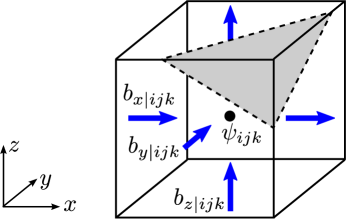
Figure 3: An example of cut cell $ijk$. The shaded region is conductor. We calculate the discrete divergence of $\bf B$ by summing the magnetic fluxes out of the unshaded volume and dividing by the unshaded volume. Since the normal magnetic field is zero on the conducting surface, that outward flux is ignored.

With Dey–Mittra boundaries, the new eigenproblem for the discrete vector Laplacian is then

$$\left({\rm A^{-1}CLC^{\rm T}+D^{\rm T}V^{-1}DA}\right)\mathbf{b}^{\prime}={k^{\prime}}^{2}\mathbf{b}^{\prime}.$$ (17)

Conveniently, the modified Dey–Mittra divergence operator has also guaranteed that eigenmodes of Eq. (5) with $k^{2}\neq 0$ (electromagnetic eigenmodes) are also eigenmodes of Eq. (17) since ${\rm DA}\mathbf{b}=0$ when $\mathbf{b}$ is an eigenmode of Eq. (5); in fact, the inverse volume fraction matrix is irrelevant for this purpose—setting it equal to the identity would also ensure that electromagnetic eigenmodes are unchanged from Eq. (5) to Eq. (17). However, as we will see in the numerical results section, the accurate calculation of the volume fractions is essential for good performance of multigrid preconditioners.

5.2 Conditioning and projecting

We have found it quite difficult to invert the left-hand side of Eq. 17; however, if we multiply both sides by the area fraction matrix, A, then inversions using multigrid converge very quickly. We believe this is primarily due to ill-conditioning of the matrix in Eq. 17 resulting from large elements in ${\rm A}^{-1}$ and ${\rm V}^{-1}$. Applying the spectral shift and inversion to the A-transformed system gives

$$\left({\rm CLC^{\rm T}+AD^{\rm T}V^{-1}DA}-\sigma{\rm A}\right)^{-1}{\rm A}\mathbf{b}^{\prime}=\frac{1}{{k^{\prime}}^{2}-\sigma}\mathbf{b}^{\prime}.$$ (18)

It was also noted by one of our reviewers that the matrix in Eq. 18 is symmetric, which may further help the linear solver.

As with the Yee scheme in vacuum, the eigenmodes with nonzero divergence must be removed (post-inversion) from the range of the vector Laplacian. Let the inner product on the discrete Yee magnetic field be

$$(\mathbf{b}_{1}^{\prime},\mathbf{b}_{2}^{\prime})\equiv{\mathbf{b}_{1}^{\prime}}^{\rm T}{\rm A}\mathbf{b}_{2}^{\prime}.$$ (19)

then we can write an arbitrary discrete magnetic field vector $\mathbf{b}^{\prime}$, as the Helmholtz decomposition

$$\mathbf{b}^{\prime}={\rm A^{-1}CL}\mathbf{e}+{\rm D}^{\rm T}\psi$$ (20)

where $\mathbf{e}$ is a discrete Yee electric field vector and $\psi$ is some cell-centered scalar field (the two parts are orthogonal under the inner product of Eq. 19). For a general vector, $\mathbf{b}^{\prime}$, with the above decomposition, the following projection operator will eliminate the part derived from the gradient matrix:

$${\rm P}_{DM}\equiv{\rm I-D^{T}(DAD^{T})^{-1}DA}$$ (21)

where I is the identity matrix. In all of our numerical tests, the matrix $\rm DAD^{T}$ was easily inverted by multigrid. Generally, we have found that if the linear solver can invert the vector Laplacian, it can invert the scalar Laplacian in Eq. 21 in a shorter time and in fewer iterations.

The final transformed system to be diagonalized iteratively is

$$\left({\rm I-D^{T}(DAD^{T})^{-1}DA}\right)\left({\rm CLC^{\rm T}+AD^{\rm T}V^{-1}DA}-\sigma{\rm A}\right)^{-1}{\rm A}\mathbf{b}^{\prime}=\frac{1}{{k^{\prime}}^{2}-\sigma}\mathbf{b}^{\prime}$$ (22)

The largest eigenvalues of the above matrix now correspond to ${k^{\prime}}^{2}\approx\sigma$, are relatively well-separated, and are purely electromagnetic (since the projection operator zeros the eigenvalues of modes with nonzero divergence).

5.3 A transformation to resemble Yee

It was observed by one of our reviewers that Eq. 22 can be written in a more compact form that makes a stronger connection with the Yee scheme. If we let

$$\tilde{\rm D}={\rm V}^{-1/2}{\rm DA}^{1/2}\quad\tilde{\rm C}={\rm A}^{-1/2}{\rm CL}^{1/2}\quad\tilde{\bf b}={\rm A}^{1/2}{\bf b}$$ (23)

then left-multiplying Eq. 22 by ${\rm A}^{1/2}$ gives

$$\left({\rm I-\tilde{D}^{T}(\tilde{D}\tilde{D}^{T})^{-1}\tilde{D}}\right)\left({\rm\tilde{C}\tilde{C}^{T}+\tilde{D}^{T}\tilde{D}}-\sigma{\rm I}\right)^{-1}\tilde{\mathbf{b}}^{\prime}=\frac{1}{{k^{\prime}}^{2}-\sigma}\tilde{\mathbf{b}}^{\prime}$$ (24)

which mimics Eq. 14. The transformations of Eq. 23 also compactly represent the vector identities and Helmholtz decomposition for the Dey–Mittra algorithm:

$${\rm\tilde{D}\tilde{C}} ={\rm\tilde{C}^{T}\tilde{D}^{T}}=0$$ (25)

$$\tilde{\bf b}^{\prime} ={\rm\tilde{C}}{\bf e}+{\rm\tilde{D}^{T}}\psi,$$ (26)

respectively.

Unfortunately, numerical tests show that the elegant symmetric form of Eq. 24 ruins convergence, supporting the argument that the inflated elements of the ${\rm A}^{-1/2}$ operator within $\tilde{C}$ are to blame (rather than overall operator symmetry). The form in Eq. 22 was used to obtain the following numerical results.

6 Numerical results

Our eigensolver makes extensive use of the trilinos linear algebra framework [25] to solve Eq. 22. Specifically, we use the block Krylov-Schur routine from the Anasazi package for the outer eigensolver iterations [26, 27], the GMRES linear solver from the AztecOO package for matrix inversions [28], and the algebraic multigrid (AMG) tool from the ML package as a preconditioner for the GMRES solver [22, 29]. Within the AMG method, we use the polynomial-based multilevel smoother (of order 1) as described in [30] which exhibits good parallel performance (e.g. as compared with popular Gauss-Seidel smoothers) since only matrix-vector multiplications are required. The multigrid preconditioner used the V-cycle; therefore, the smoother was applied twice at each level per iteration (once on the way to coarser grids, and once on the way back to the original fine grid). The coarsest level was treated the same as any other multigrid level. The vector and scalar Laplacians to be inverted in Eq. 22 were formed explicitly, then passed to the ML algorithm.

Cubic grid cells were used throughout the following tests ($\Delta x=\Delta y=\Delta z$).

Most simulations were performed on Hopper, the Cray XE6 supercomputer at the National Energy Research Scientific Computing Center.

6.1 Performance: spherical cavity

In Table 1, we compare the performance of the linear solver (the bottleneck) on a model problem (cubic domain with perfectly-conducting boundaries) with a simple problem requiring the Dey–Mittra algorithm (the spherical cavity). No cut faces were neglected in the sphere simulation; the smallest area fraction encountered was $6\times 10^{-4}$. The cubic domain had arbitrary side-length $L$, and the spherical cavity had radius $0.49L$. Eigensolves were performed for the lowest three modes; each eigensolve took about 20 outer iterations to complete (20 vector/scalar Laplacian inversions). The figures in Table 1 are averages over these 20 inversions.

The multigrid complexity is defined as

$${\rm complexity}=\frac{\sum_{i=1}^{N}\operatorname{nnz}({\rm A}_{i})}{\operatorname{nnz}({\rm A}_{1})}$$ (27)

where A_i is the linear system matrix on multigrid level $i$ (with $i=1$ representing the finest level) and the nnz() operator produces the number of nonzero elements in the operand matrix.

Table 1: Linear solver benchmarks for the inversion of the vector Laplacian without (cube) and with (sphere) Dey–Mittra boundaries. One polynomial (order 1) smoother sweep per multigrid level. Component count is the number of magnetic field components. Inversions were performed to $10^{-6}$ accuracy. For every simulation, processor domains were 16x16x16 cells.

	Cube			Sphere
Component count	12,285	98,301	786,429	7,815	55,398	414,489
Avg. iteration count	8.8	9.3	9.6	10.0	10.1	10.5
Convergence rate	0.21	0.22	0.24	0.25	0.25	0.27
Multigrid levels	3	4	4	3	4	4
Multigrid complexity	1.5	1.6	1.6	1.6	1.7	1.8
Domain decomposition	1x1x1	2x2x2	4x4x4	1x1x1	2x2x2	4x4x4

Iteration counts are strikingly similar between the model problem and the spherical cavity. However, if the inverse volume matrix is left out of Eq. 22, vector Laplacian inversions do not converge in a reasonable number of iterations (for a GMRES basis size of 40, more than 10 restarts were required—thus, more than 400 total iterations). To examine the importance of the inverse volume matrix on the linear solver performance, we perturbed our accurate cell volume calculations (for cut cells only) in the following way

$$\tilde{v}_{ijk}=10^{f_{ijk}\epsilon}v_{ijk}$$ (28)

where $v_{ijk}$ is the accurate volume, $f_{ijk}$ is a random factor between $-1$ and 1, and $\epsilon$ is an “order of magnitude” parameter (e.g. for $\epsilon=1$, the volume can be wrong by up to an order of magnitude).

We also tested errors that are likely to result from a simple subsampling volume calculation routine. In this case, the model was

$$\tilde{v}_{ijk}=v_{ijk}+f_{ijk}\Delta v$$ (29)

where $v_{ijk}$ is the accurate volume, $f_{ijk}$ is a random factor between $-1$ and 1, and $\Delta v$ is the perturbation (or subsample) volume.

Table 2 shows the effect of these errors on linear solver convergence for different values of $\epsilon$ and $\Delta v/v_{\rm vac}$ where $v_{\rm vac}=\Delta x\Delta y\Delta z$, and indicates the importance of a good volume estimate (assuming accurate area fraction calculations). For example, according to Table 2, a subsampling routine with 10 samples per dimension of a grid cell (1000 cubic subvolumes) could lead to very poor convergence. Our volume calculation method breaks cut-cell volumes into tetrahedral subvolumes that conform to the embedded surface (the volumes of which are easy to calculate individually); therefore, our method converges to the exact cut-cell volume for smooth boundaries.

Table 2: Effect of cut-cell volume calculation errors on linear solver convergence for the spherical cavity problem. Each $\epsilon$ and $\Delta v$ was simulated three times; the average iteration count from each was then averaged over these three simulations. Simulation domain was 32x32x32. Inversions were performed to $10^{-6}$ accuracy.

Error from Eq. 28
$\epsilon$	0.1	0.3	0.5	1	2	3
Avg. iteration count	10	11	13	24	74	220
Error from Eq. 29
$\Delta v/v_{\rm vac}$	$10^{-5}$		$10^{-4}$		$10^{-3}$
Avg. iteration count	10		50		91

6.2 Dey–Mittra frequency and field convergence

This section compares frequencies and surface fields in the spherical cavity calculated by the Dey–Mittra algorithm with their analytic counterparts for varying $a_{\rm min}/a_{\rm vac}$ (where $a_{\rm vac}=\Delta x\Delta y=\Delta y\Delta z=\Delta x\Delta z$ because cells are cubic). For these simulations, parity symmetry was invoked to reduce the simulation domain to the positive $x$, $y$, and $z$ octant (sphere centered at the origin). Boundaries at $x=0$, $y=0$, and $z=0$ (the symmetry planes) were set as perfectly-conducting. The lowest eigenmode was analyzed which, for the above symmetry, corresponded to the TM₀₃₂ spherical cavity mode [31].

Relative frequency errors were calculated by

$$\varepsilon_{\rm freq}=\frac{|\omega-\omega_{0}|}{\omega_{0}}$$ (30)

where $\omega$ is the calculated angular frequency and $\omega_{0}$ is the analytic angular frequency. All plots in this section use as the abscissa the resolution relative to the vacuum wavelength of the mode, where the vacuum wavelength is defined as $\lambda_{\rm vac}=2\pi c/\omega_{0}$. Figure 4 shows the second-order convergence of the pure Dey–Mittra algorithm and the first-order error effect introduced by neglecting cut faces. One should also note the difference in relative error at low resolutions, which can be significant.

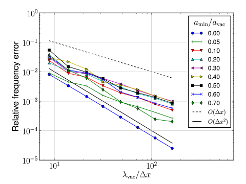
Figure 4: Color online. Convergence of TM₀₃₂ resonant frequency in the spherical cavity as a function of resolution and $a_{\rm min}/a_{\rm vac}$. The unaltered Dey–Mittra algorithm is clearly second-order, while neglecting faces results in eventual first-order convergence (as similarly reported in [2])

Electric fields near the surface of the spherical cavity were calculated and compared with analytic solutions [31]. Since interpolation of fields to the metal boundary is equivocal and nontrivial, we analyzed “surface” fields on a shell a radial distance $3\Delta x$ away from the boundary where standard trilinear interpolations are appropriate. Because surface fields were analyzed a fixed number of grid cell widths from the boundary, the physical distance from the boundary decreased as resolution increased. Before surface fields were compared, analytic and simulated fields were scaled to have the same $\ell_{2}$-norm where the norm was calculated by sampling each field over the same collection of points filling the cavity volume.

The relative $\ell_{2}$ errors of the computed eigenmodes are,

$$\varepsilon_{\rm field}=\sqrt{\frac{\sum_{i}\big{|}{\bf e}({\bf x}_{i})-{\bf E}({\bf x}_{i})\big{|}^{2}}{\sum_{i}\big{|}{\bf E}({\bf x}_{i})\big{|}^{2}}}$$ (31)

where the ${\bf x}_{i}$ are test points on a shell, ${\bf E}({\bf x})$ is the analytic eigenmode evaluated at $\bf x$, and ${\bf e}({\bf x})$ is the computed eigenmode interpolated to the point $\bf x$ (using trilinear interpolation). Figure 5 shows the results for the TM₀₃₂ spherical cavity mode. Surface fields ultimately do not converge when faces are neglected, yet converge with nearly second-order error for the pure Dey–Mittra algorithm.

Figure 5: Color online. Convergence of TM₀₃₂ surface fields in the spherical cavity as a function of resolution and $a_{\rm min}/a_{\rm vac}$.

6.3 Performance: TESLA cavity

Our eigensolver’s performance (i.e. the linear solver performance) was also tested on a modern accelerator cavity problem—the TESLA superconducting cavity [32] (see Fig. 6). One quarter of the nine-cell cavity was simulated where the $x=0$ and $y=0$ boundary planes were perfect magnetic conductor (the $z$-direction is the long direction); therefore, the TM₀₁₀-like accelerating modes were found at the lowest frequencies ($\approx 1.3$ GHz). Three different resolutions were tested on the TESLA cavity shown in Fig. 6; additionally, a cryomodule was simulated, which consists of 8 TESLA cavities strung end-to-end in the $z$-direction.

Simulation results are summarized in Table 3; the first 3 columns refer to the single TESLA cavity simulations and the last column the cryomodule. For the TESLA cavity simulations, the maximum eigensolver Krylov basis size (before a restart occurs) was 50, and the lowest 9 eigenmodes were found. Only 32 outer eigensolver iterations were required (no restarts necessary) at each resolution. For the cryomodule simulation, to save resources on Hopper (supercomputer at NERSC), we restricted the eigensolver to find only the lowest 3 eigenmodes and disallowed eigensolver restarts; 30 eigensolver iterations were performed.

In Table 3, the estimated relative frequency error of the accelerating mode is given by $\varepsilon_{\rm freq}=(f\Delta x/c)^{2}$ where $f=1.3$ GHz.

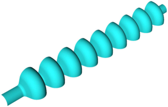
Figure 6: Simulated quarter section of the 9-cell TESLA superconducting accelerator cavity. Beam tubes terminate at conducting walls. The length of the cavity is 1.38 meters.

Table 3: Performance of linear solver during an eigensolve of the TESLA cavity. One polynomial (order 1) smoother sweep per level per traverse (same as spherical cavity simulations). Inversions performed to $10^{-6}$ accuracy. Numbers in the last column apply to a cryomodule simulation—eight TESLA cavities end-to-end.

Comp. count ($\times 10^{6}$)	0.8	6.4	50.2	520 (cryo)
Grid cell $\Delta x$ (mm)	2.9	1.4	0.72	0.66
Estimated $\varepsilon_{\rm freq}$	$2\times 10^{-4}$	$4\times 10^{-5}$	$1\times 10^{-5}$	$8\times 10^{-6}$
Avg. iteration count	11.8	11.9	12.6	13.9
Convergence rate	0.31	0.31	0.33	0.37
Multigrid complexity	1.6	1.6	1.6	1.6
Multigrid levels	5	5	5	5
Domain decomposition	1x1x12	2x2x24	4x4x48	4x4x418

7 Conclusion

We derived a matrix transformation for the Dey–Mittra curl-curl operator that allows for efficient inversion by multigrid methods. In fact, the performance of multigrid applied to our custom Dey–Mittra vector Laplacian nearly equals the performance of multigrid on the model problem (grid-aligned cubic domain). As a result, we developed an efficient shift-and-invert eigensolver for Maxwell’s equations in resonant cavities. Eigensolver performance was demonstrated on the simple spherical cavity and the TESLA superconducting cavity. This eigensolver is open-sourced at https://github.com/bauerca/maxwell.

The effects on accuracy of neglecting small cut faces in the Dey–Mittra algorithm were also investigated. An analysis of Dey–Mittra surface fields showed the stagnation of convergence (when faces are neglected) for fields a fixed number of grid cells away from conducting boundaries; in contrast, if all faces are kept (which is the case for our new eigensolver), surface field convergence is nearly second-order.

References

- [1] S. Dey, R. Mittra, A locally conformal finite-difference time-domain (FDTD) algorithm for modeling three-dimensional perfectly conducting objects, Microwave and Guided Wave Letters, IEEE [see also IEEE Microwave and Wireless Components Letters] 7 (9) (1997) 273–275.
- [2] C. Nieter, J. R. Cary, G. R. Werner, D. N. Smithe, P. H. Stoltz, Application of Dey–Mittra conformal boundary algorithm to 3D electromagnetic modeling, Journal of Computational Physics 228 (2009) 7902–7916.
- [3] K. Yee, Numerical solution of inital boundary value problems involving maxwell’s equations in isotropic media, IEEE Transactions on antennas and propagation 14 (3) (1966) 302–307.
- [4] R. Hiptmair, Multigrid method for Maxwell’s equations, SIAM Journal on Numerical Analysis 36 (1) (1998) 204–225.
- [5] P. Bochev, C. Garasi, J. Hu, A. Robinson, R. Tuminaro, An improved algebraic multigrid method for solving Maxwell’s equations, SIAM Journal on Scientific Computing 25 (2) (2004) 623–642.
- [6] M. Clemens, S. Feigh, T. Weiland, Construction principles of multigrid smoothers for curl-curl equations, IEEE Transactions on Magnetics 41 (5) (2005) 1680–1683.
- [7] P. Arbenz, R. Geus, Multilevel preconditioned iterative eigensolvers for Maxwell eigenvalue problems, Applied Numerical Mathematics 54 (2) (2005) 107–121.
- [8] J. Hu, R. Tuminaro, P. Bochev, C. Garasi, A. Robinson, Toward an h-independent algebraic multigrid method for maxwell’s equations, SIAM Journal on Scientific Computing 27 (5) (2006) 1669–1688.
- [9] T. Kolev, P. Vassilevski, Parallel auxiliary space amg for h (curl) problems, J. Comput. Math 27 (5) (2009) 604–623.
- [10] W. Briggs, S. McCormick, et al., A multigrid tutorial, Vol. 72, Society for Industrial Mathematics, 2000.
- [11] A. Taflove, S. Hagness, Computational electrodynamics, Artech house Boston, 1995.
- [12] G. R. Werner, J. R. Cary, A stable FDTD algorithm for non-diagonal, anisotropic dielectrics, Journal of Computational Physics 226 (1) (2007) 1085–1101.
- [13] T. Weiland, A discretization model for the solution of Maxwell’s equations for six-component fields, Archiv fuer Elektronik und Uebertragungstechnik 31 (1977) 116–120.
- [14] M. Clemens, T. Weiland, Discrete electromagnetism with the finite integration technique, Progress in Electromagnetics Research, PIER 32 (2001) 65–87.
- [15] I. Zagorodnov, R. Schuhmann, T. Weiland, A uniformly stable conformal fdtd-method in cartesian grids, International Journal of Numerical Modelling: Electronic Networks, Devices and Fields 16 (2) (2003) 127–141.
- [16] I. Zagorodnov, R. Schuhmann, T. Weiland, Conformal fdtd-methods to avoid time step reduction with and without cell enlargement, Journal of Computational Physics 225 (2) (2007) 1493–1507.
- [17] A. Tornberg, B. Engquist, Consistent boundary conditions for the yee scheme, Journal of Computational Physics 227 (14) (2008) 6922–6943.
- [18] B. Engquist, J. Häggblad, O. Runborg, On energy preserving consistent boundary conditions for the yee scheme in 2d, BIT Numerical Mathematics (2011) 1–23.
- [19] G. Stewart, Matrix Algorithms: Eigensystems, Vol. 2, Society for Industrial Mathematics, 2001.
- [20] H. van der Vorst, Computational methods for large eigenvalue problems, Handbook of numerical analysis 8 (2002) 3–179.
- [21] R. Grimes, J. Lewis, H. Simon, A shifted block lanczos algorithm for solving sparse symmetric generalized eigenproblems, SIAM J. Matrix Anal. Appl 15 (1991) 1–45.
- [22] P. Vaněk, J. Mandel, M. Brezina, Algebraic multigrid by smoothed aggregation for second and fourth order elliptic problems, Computing 56 (3) (1996) 179–196.
- [23] P. Bochev, J. Hu, C. Siefert, R. Tuminaro, An Algebraic Multigrid Approach Based on a Compatible Gauge Reformulation of Maxwell’s Equations, SIAM Journal on Scientific Computing 31 (2008) 557.
- [24] P. Bochev, J. Hyman, Principles of mimetic discretizations of differential operators, Compatible spatial discretizations (2006) 89–119.
- [25] M. A. Heroux, R. A. Bartlett, V. E. Howle, R. J. Hoekstra, J. J. Hu, T. G. Kolda, R. B. Lehoucq, K. R. Long, R. P. Pawlowski, E. T. Phipps, A. G. Salinger, H. K. Thornquist, R. S. Tuminaro, J. M. Willenbring, A. Williams, K. S. Stanley, An overview of the trilinos project, ACM Trans. Math. Softw. 31 (3) (2005) 397–423. doi:http://doi.acm.org/10.1145/1089014.1089021.
-
[26]
G. Stewart, A
krylov–schur algorithm for large eigenproblems, SIAM Journal on Matrix
Analysis and Applications 23 (3) (2002) 601–614.
arXiv:http://epubs.siam.org/doi/pdf/10.1137/S0895479800371529, doi:10.1137/S0895479800371529.
URL http://epubs.siam.org/doi/abs/10.1137/S0895479800371529 -
[27]
C. G. Baker, U. L. Hetmaniuk, R. B. Lehoucq, H. K. Thornquist,
Anasazi software for the
numerical solution of large-scale eigenvalue problems, ACM Trans. Math.
Softw. 36 (3) (2009) 13:1–13:23.
doi:10.1145/1527286.1527287.
URL http://doi.acm.org/10.1145/1527286.1527287 - [28] Y. Saad, M. Schultz, Gmres: A generalized minimal residual algorithm for solving nonsymmetric linear systems., SIAM J. Sci. Stat. Comput. 7 (3) (1986) 856–869.
- [29] M. Gee, C. Siefert, J. Hu, R. Tuminaro, M. Sala, ML 5.0 smoothed aggregation user’s guide, Tech. Rep. SAND2006-2649, Sandia National Laboratories (2006).
- [30] M. Adams, M. Brezina, J. Hu, R. Tuminaro, Parallel multigrid smoothing: polynomial versus gauss–seidel, Journal of Computational Physics 188 (2) (2003) 593–610.
- [31] J. D. Jackson, Classical Electrodynamics, 3rd Edition, 3rd Edition, John Wiley and Sons, Inc., 1999.
-
[32]
B. Aune, R. Bandelmann, D. Bloess, B. Bonin, A. Bosotti, M. Champion,
C. Crawford, G. Deppe, B. Dwersteg, D. A. Edwards, H. T. Edwards,
M. Ferrario, M. Fouaidy, P.-D. Gall, A. Gamp, A. Gössel, J. Graber,
D. Hubert, M. Hüning, M. Juillard, T. Junquera, H. Kaiser, G. Kreps,
M. Kuchnir, R. Lange, M. Leenen, M. Liepe, L. Lilje, A. Matheisen, W.-D.
Möller, A. Mosnier, H. Padamsee, C. Pagani, M. Pekeler, H.-B. Peters,
O. Peters, D. Proch, K. Rehlich, D. Reschke, H. Safa, T. Schilcher,
P. Schmüser, J. Sekutowicz, S. Simrock, W. Singer, M. Tigner, D. Trines,
K. Twarowski, G. Weichert, J. Weisend, J. Wojtkiewicz, S. Wolff, K. Zapfe,
Superconducting
tesla cavities, Phys. Rev. ST Accel. Beams 3 (2000) 092001.
doi:10.1103/PhysRevSTAB.3.092001.
URL http://link.aps.org/doi/10.1103/PhysRevSTAB.3.092001