root’s barrier, viscosity solutions of obstacle problems and reflected FBSDEs

Abstract.

We revisit work of Rost [49], Dupire [22] and Cox–Wang [16] on connections between Root’s solution of the Skorokhod embedding problem and obstacle problems. We develop an approach based on viscosity sub- and supersolutions and an accompanying comparison principle. This gives a complete characterization of (reversed) Root barriers and also leads to new proofs of the existence as well as the minimality of Root solutions by pure PDE methods. The approach is self-contained, constructive and also general enough to cover martingale diffusions with degenerate elliptic or time-dependent volatility; it also provides insights about the dynamics of general Skorokhod embeddings by identifying them as supersolutions of certain nonlinear PDEs.

1. Introduction

This article revisits the dynamics of the Skorokhod embedding problem from a viscosity PDE perspective with an emphasis on Root’s solution. That is, under mild assumptions on the probability measures $\mu,\nu$ on $\mathbb{R}$ and the volatility coefficient $\sigma$, we are interested in finding a (non-randomized) stopping time $\tau$ such that

(SEP) $$\left\{\begin{array}[]{rcl}dX_{t}&=&\sigma\left(t,X_{t}\right)dB_{t},\,X_{0}\sim\mu,\\ X_{\tau}&\sim&\nu\text{ and }X^{\tau}=\left(X_{t\wedge\tau}\right)_{t\geq 0}\text{ is uniformly integrable.}\end{array}\right.$$

For general background on (SEP) and its applications we refer to Hobson and Obłój [42, 31]. In the Brownian case, $\sigma\equiv 1$ and $\mu=\delta_{0}$, Root showed in 1969 [45] that the stopping time $\tau$ can be realized as the first hitting of a closed time-space set, the so-called Root barrier,

$$R\subset\left[0,\infty\right]\times\left[-\infty,\infty\right]$$

by the time-space process $t\mapsto\left(t,X_{t}\right)$. Further important developments are due to Rost: firstly, he showed that Root’s solution minimizes

(1) $$\mathbb{E}\left[\int_{t\wedge\tau}^{\tau}f\left(X_{s}\right)ds\right]\,\,\,\forall f\geq 0,\forall t\geq 0$$

among all solutions of (SEP), [49]; secondly, he gave a new existence proof of Root’s barrier by using potential theory that generalizes to time-homogenous Markov processes [49, 46]; thirdly, he showed that there exist another barrier $R^{\text{rev}}$ that solves (SEP) and minimizes the diffusion of $X$, [48, 47]. Another important contribution concerning the uniqueness of the barrier $R$ was made by Loynes [38].

Already for Brownian motion it was not known how to construct $R$ except for a handful of simple cases. A completely new perspective that led to a revived interest in (SEP) came from the management of risk in mathematical finance. It was started by work of Hobson [32] that showed how model-independent bounds of exotic options can be obtained by “extremal solutions” of (SEP). Motivated by this, Dupire [22] showed formally that the barrier $R$ is naturally linked to a nonlinear PDE that allows to solve for $R$. This was further developed by Cox–Wang [16] who use a variational formulation, as developed in the 1970’s by Bensoussan–Lions et. al. [10], to calculcate $R$ in case its existence is guaranteed by these classic results of Root and Rost. More recently, Gassiat–Mijatovic–Oberhauser [28] studied the barrier via integral equations, Cox–Peskir [17] studied reversed barriers, Beiglböck–Cox–Huesmann [9] develop an optimal transport perspective of (SEP) and Kleptsyn–Kurtzmann [37] use Root’s barrier to construct a counter-example to the Cantelli conjecture; there are also many more developments beyond the context of Root type solutions, see for example [1, 2, 3, 27, 29, 44] for interesting recent progress.

This article takes the PDE approach further by giving a self-contained approach to the embedding problem based on viscosity solutions. The parabolic comparison principle plays the key role. It allows us to provide new proofs of firstly, the existence of a Root solution, and secondly, its minimizing property (1). In the Brownian, or homogenous diffusion case, this recovers the classic results of Root and Rost [45, 49] by constructive methods and provides insights about the general dynamics of (SEP); in the time-inhomogenous case, already the existence and minimality results themselves are new to the best of our knowledge and would be hard to obtain otherwise, since the classic approaches break down; however in the current setup they become simple consequences of a PDE existence and a comparison of sub- and supersolutions; see Theorem 1, Theorem 2 and Theorem 3. Moreover, the PDE methods we introduce also cover Rost’s reversed Root barriers, where already for the Brownian case, they might be an attractive, constructive(!) alternative to the classic “filling scheme” [14, 47] proof that relies on deep results from potential theory.

Structure of the article.

In Section 2 we introduce notation and our assumptions on $\left(\sigma,\mu,\nu\right)$. We then give our first main result, Theorem 1, which states that any solution of the Skorokhod embedding problem (SEP) is a viscosity supersolution of a certain obstacle PDE. If one thinks in potential theoretic terms, this can be seen as the PDE version of Rost’s approach [49] to (SEP) via excessive functions of Markov processes.

In Section 3 we introduce an extension of Loyne’s notion of regular Root barriers which allows to deduce the uniqueness of such barrier solutions. We then present our second main result, Theorem 2, which shows a one-on-one correspondence of regular Root barriers and viscosity solutions. This complete characterization allows us to firstly, prove the existence of Root barriers via PDE existence, Corollary 1, and secondly, show that the minimizing property (1) is a simple consequence of a parabolic comparison result, Theorem 4. We also briefly revisit and leverage results about reflected FBSDEs [24] which allows to use Monte-Carlo methods to calculate barriers and gives another interpretation as a stopping problem. We conclude this section by showing, how our approach also gives existence and minimalty proofs of Rost’s reversed barriers.

In Section 4 we implement numerical schemes to solve for the barrier and apply the Barles–Souganidis method to get convergence (+rates of convergence) which might be useful for practitioners in financial mathematics (bounds on options on variance).

2. Skorokhod embeddings as supersolutions

2.1. Notation and Assumptions

Denote with $\left(\Omega,\mathcal{F},\left(\mathcal{F}_{t}\right),\mathbb{P}\right)$ a filtered probability space that satisfies the usual conditions and carries a standard Brownian motion $B$ and a real-valued random variable $X_{0}\sim\mu$ that is independent of $B$. We work under the following assumption on $\left(\sigma,\mu,\nu\right)$.

Assumption 1.

$\mu$ and $\nu$ are measures on $\left(\mathbb{R},\mathcal{B}\left(\mathbb{R}\right)\right)$ that have a first moment and are in convex order, i.e.

$$u_{\nu}\left(x\right):=-\int_{\mathbb{R}}\left|x-y\right|\nu\left(dy\right)\leq-\int_{\mathbb{R}}\left|x-y\right|\mu\left(dy\right)=:u_{\mu}\left(x\right)\,\,\forall x\in\mathbb{R}.$$

Let $\sigma\in C\left(\left[0,\infty\right)\times\mathbb{R},\mathbb{R}\right)$ be Lipschitz in space and of linear growth, both uniformly in time, that is

(2) $$\sigma_{Lip}:=\sup_{t\in\left[0,\infty\right)}\sup_{x\neq y}\frac{\left|\sigma\left(t,x\right)-\sigma\left(t,y\right)\right|}{\left|x-y\right|}<\infty\text{ \,\ and\,\ }\sigma_{LG}:=\sup_{t\in\left[0,\infty\right)}\sup_{x\in\mathbb{R}}\frac{\left|\sigma\left(t,x\right)\right|}{1+\left|x\right|}<\infty.$$

Further assume local ellipticity in the sense that for each compact $K\subset\left\{x:u_{\mu}\left(x\right)\neq u_{\nu}\left(x\right)\right\}$, there exists some $c_{K}>0$ s.t.

$$\sigma(t,x)\geq c_{K}>0,\;\;\;\;\forall t\geq 0,x\in K.$$

The need for above assumptions is intuitively clear: convex order of $\mu,\nu$ is necessary by classic work of Chacon and Kellerer about the marginals of martingales [35, 12]; however we only assume first moments which is already for the Brownian case, $\sigma\equiv 1$, weaker than Root’s assumption [45]. Linear growth and Lipschitz property of $\sigma$ are natural since we describe the evolution of the law of the strong solution $X^{\tau}$ by PDEs; some nondegeneracy of the diffusion is clearly required to be able to transport the mass $\mu$ to $\nu$. (Note that what we call “local ellipticity” covers degenerate elliptic diffusions, e.g. for geometric Brownian motion, $\sigma(x)=x$ our assumption is fulfilled if and only if the support of $\nu$ is contained in the positive halfline which is in this case the sharp condition).

Definition 1.

Let $\left(\sigma,\mu,\nu\right)$ fulfill Assumption 1. We denote with $\operatorname{\text{SEP}_{\sigma,\mu,\nu}}$ the set of $\left(\mathcal{F}_{t}\right)$-stopping times $\tau$ that solve the Skorokhod embedding problem

$$\left\{\begin{array}[]{rcl}dX_{t}&=&\sigma\left(t,X_{t}\right)dB_{t},\,X_{0}\sim\mu,\\ X_{\tau}&\sim&\nu\text{ and }X^{\tau}=\left(X_{t\wedge\tau}\right)_{t\geq 0}\text{ is uniformly integrable.}\end{array}\right.$$

2.2. Recall on viscosity theory

We briefly recall standard concepts from viscosity theory; for more details see [19, 26].

Definition 2.

Let $\mathcal{O}$ be a locally compact subset of $\mathbb{R}$ and denote $\mathcal{O}_{T}=\left(0,T\right)\times\mathcal{O}$ and $\overline{\mathcal{O}}_{T}=\left[0,T\right]\times\mathcal{O}$ for a given $T\in\left(0,\infty\right]$. Consider a function $u:\mathcal{O}_{T}\rightarrow\mathbb{R}$ and define for $\left(s,z\right)\in\mathcal{O}_{T}$ the parabolic superjet $\mathcal{P}_{\mathcal{O}}^{2,+}u\left(s,z\right)$ as the set of triples $\left(a,p,m\right)\in\mathbb{R}\times\mathbb{R}\times\mathbb{R}$ which fulfill

(3) $$u\left(t,x\right) \leq u\left(s,z\right)+a\left(t-s\right)+\left\langle p,x-z\right\rangle$$

$$+\frac{1}{2}\left\langle m\left(x-z\right),x-z\right\rangle+o\left(\left|t-s\right|+\left|x-z\right|^{2}\right)\text{ as }\mathcal{O}_{T}\ni\left(t,x\right)\rightarrow\left(s,z\right)$$

Similarly we define the parabolic subjet $\mathcal{P}_{\mathcal{O}}^{2,-}u\left(s,z\right)$ such that $\mathcal{P}_{\mathcal{O}}^{2,-}u=-\mathcal{P}_{\mathcal{O}}^{2,+}\left(-u\right)$.

Definition 3.

A function $F:\mathcal{O}_{T}\times\mathbb{R}\times\mathbb{R}\times\mathbb{R}\times\mathbb{R}\rightarrow\mathbb{R}$ is proper if $\forall\left(t,x,a,p\right)\in\mathcal{O}_{T}\times\mathbb{R}\times\mathbb{R}$

$$F\left(t,x,r,a,p,m\right)\leq F\left(t,x,s,a,p,m^{\prime}\right)\,\,\forall m\geq m^{\prime},\,s\geq r.$$

Denote the real-valued, upper semicontinuous functions on $\overline{\mathcal{O}}_{T}$ with $USC\left(\overline{\mathcal{O}}_{T}\right)$ and the lower semicontinuous functions with $LSC\left(\overline{\mathcal{O}}_{T}\right)$. A subsolution of the (forward problem)

(4) $$\left\{\begin{array}[]{rcl}F\left(t,x,u,\partial_{t}u,Du,D^{2}u\right)&=&0\\ u\left(0,.\right)&=&u_{0}\left(.\right)\end{array}\right.$$

is a function $u\in USC\left(\overline{\mathcal{O}}_{T}\right)$ such that

$$F\left(t,x,u,a,p,m\right) \leq 0\text{ for }\left(t,x\right)\in\mathcal{O}_{T}\text{ and }\left(a,p,m\right)\in\mathcal{P}_{\mathcal{O}}^{2,+}u\left(t,x\right)$$

$$u\left(0,.\right) \leq u_{0}\left(.\right)\text{ on }\mathcal{O}$$

The definition of a supersolution follows by replacing $USC\left(\overline{\mathcal{O}}_{T}\right)$ by $LSC\left(\overline{\mathcal{O}}_{T}\right)$, $\mathcal{P}_{\mathcal{O}}^{2,+}$ by $\mathcal{P}_{\mathcal{O}}^{2,-}$ and $\leq$ by $\geq.$ If $u$ is a supersolution of (4) then we also say that $F\left(t,x,u,\partial_{t}u,Du,D^{2}u\right)\geq 0,\,u\left(0,x\right)\geq u_{0}\left(x\right)$ holds in viscosity sense (similar for subsolutions). Similarly we call a function $v$ a viscosity (sub-,super-) solution of the backward problem

(5) $$\left\{\begin{array}[]{rcl}G\left(t,x,v,\partial_{t}v,Dv,D^{2}v\right)&=&0\\ v\left(T,.\right)&=&v_{T}\left(.\right)\end{array}\right.$$

if

$$G\left(t,x,v,a,p,m\right) \leq 0\text{ for }\left(t,x\right)\in\mathcal{O}_{T}\text{ and }\left(a,p,m\right)\in\mathcal{P}_{\mathcal{O}}^{2,+}v\left(t,x\right)$$

$$v\left(0,.\right) \leq v_{T}\left(.\right)\text{ on }\mathcal{O}.$$

2.3. Skorokhod embeddings as PDE supersolutions

Chacon [13] showed that for $\tau\in\operatorname{SEP}_{\sigma,\mu,\nu}$, the potential function $u^{\tau}\left(t,x\right)\equiv-\mathbb{E}\left[\left|X_{t\wedge\tau}-x\right|\right]$ is a powerful tool to study the evolution of the law of the stopped (local) martingale $X^{\tau}=\left(X_{\tau\wedge t}\right)$. Theorem 1 captures the following intuition: $u^{\tau}$ is a concave function of $X^{\tau}$, hence we expect it to be a supersolution (in some sense) of a Fokker–Planck equation. However, $u^{\tau}$ cannot be smooth for generic Skorokhod solutions due to kinks from stopping at $u_{\nu}$. Further, since $u^{\tau}$ is the potential of the occupation measure of $X^{\tau}$ and $\tau\in\operatorname{SEP}_{\sigma,\mu,\nu}$, it follows that $u^{\tau}\left(t,.\right)$ is bounded below by the potential of the measure $\nu$ and will converge to it as $t\rightarrow\infty$. We now make this rigorous under the generality of Assumption 1.

Theorem 1.

Let $\left(\sigma,\mu,\nu\right)$ fulfill Assumption 1. Then for every $\tau\in$$\operatorname{SEP}_{\sigma,\mu,\nu}$ the function

$$u^{\tau}\left(t,x\right):=-\mathbb{E}\left[\left|X_{\tau\wedge t}-x\right|\right]$$

is a viscosity supersolution of

(6) $$\left\{\begin{array}[]{rcl}\inf\left(u-u_{\nu},\partial_{t}u-\frac{\sigma^{2}}{2}\Delta u\right)&=&0\text{ on }\left(0,\infty\right)\times\mathbb{R},\\ u\left(0,.\right)&=&u_{\mu}\left(.\right)\end{array}\right.$$

and

$$\lim_{t\rightarrow\infty}u^{\tau}\left(t,x\right)=u_{\nu}\left(x\right)\,\,\,\forall x\in\mathbb{R}.$$

Proof.

We have to show that

$$\left\{\begin{array}[]{rcl}u^{\tau}-u_{\nu}&\geq&0\text{ on }\left(0,\infty\right)\times\mathbb{R},\\ \left(\partial_{t}-\frac{\sigma^{2}}{2}\Delta\right)u^{\tau}&\geq&0\text{ on }\left(0,\infty\right)\times\mathbb{R},\\ \lim_{t\rightarrow\infty}u^{\tau}&=&u_{\nu}.\end{array}\right.$$

The first inequality follows immediately via conditional Jensen

(7) $$u^{\tau}\left(t,x\right)=-\mathbb{E}\left[\left|X_{t}^{\tau}-x\right|\right]\geq\mathbb{E}\left[\mathbb{E}\left[-\left|X_{\tau}-x\right|\lvert\mathcal{F}_{t\wedge\tau}\right]\right]=-\mathbb{E}\left[\left|X_{\tau}-x\right|\right]=u_{\nu}\left(x\right).$$

and the last one is immediate from properties of potential functions, see [13, 42]. For the second inequality we approximate $u^{\tau}$ by a sequence of regularizations $\left(u^{n}\right)_{n}$. We show that each $u^{n}$ is a supersolution of a ”perturbed version” of (6) and we conclude by sending $n\rightarrow\infty$ and using the stability of viscosity solutions.

Step 1. Convergence of $u^{n}\left(t,x\right):=\mathbb{E}\left[\psi^{n}\left(X_{t}^{\tau}-x\right)\right]$ as $n\rightarrow\infty.$
Define the sequence $\left(\psi_{n}\right)\subset C^{2}\left(\mathbb{R},\mathbb{R}\right)$ as

$$\psi_{n}\left(x\right)=\int_{0}^{x}\int_{0}^{y}n\phi\left(nz\right)dzdy\forall x\in\mathbb{R}$$

where $\phi$ is the usual Gaussian scaled to the unit disc

$$\phi\left(x\right)=\begin{cases}\exp\left(-\frac{1}{1-x^{2}}\right)&\text{for }\left|x\right|<1,\\ 0&\text{otherwise}.\end{cases}$$

Especially note that $\psi_{n}\left(.\right)\rightarrow\left|.\right|$ uniformly, $\Delta\psi_{n}\left(.\right)$ is continuous, $0\leq\Delta\psi_{n}\leq O\left(n\right)$ and $\operatorname{supp}\left(\Delta\psi_{n}\right)\subset\left[-\frac{1}{n},\frac{1}{n}\right]$ (we could replace $\psi^{n}$ by any other sequence with this properties). Further introduce

$$u^{n}\left(t,x\right) = -\mathbb{E}\left[\psi_{n}\left(X_{t}^{\tau}-x\right)\right],$$

$$u_{\nu}^{n}\left(x\right) = -\int_{\mathbb{R}}\psi^{n}\left(y-x\right)\nu\left(dy\right),$$

$$u_{\mu}^{n}\left(x\right) = -\int_{\mathbb{R}}\psi^{n}\left(y-x\right)\mu\left(dy\right).$$

Since $\psi_{n}\left(.\right)\rightarrow\left|.\right|$ uniformly we have $\mathbb{P}$-a.s.

$$\left|\psi^{n}\left(X_{.}^{\tau}-.\right)-\left|X_{.}^{\tau}-.\right|\right|_{\infty;\left[0,\infty\right)\times\mathbb{R}}=\sup_{\left(t,x\right)\in\left[0,\infty\right)\times\mathbb{R}}\left|\psi^{n}\left(X_{t}^{\tau}-x\right)-\left|X_{t}^{\tau}-x\right|\right|\rightarrow_{n\rightarrow\infty}0$$

hence we get uniform convergence of $u^{n},u_{\mu}^{n}$ and $u_{\nu}^{n}$, i.e.

$$\left|u^{n}-u\right|_{\infty;[0,\infty)\times\mathbb{R}}\rightarrow_{n}0,\qquad\left|u_{\nu}^{n}-u_{\nu}\right|_{\infty,\mathbb{R}}\rightarrow_{n}0,\qquad\text{{and}}\qquad\left|u_{\mu}^{n}-u_{\mu}\right|_{\infty,\mathbb{R}}\rightarrow_{n}0.$$

Further, by the definition of $u$ and $u^{n}$ we see that $\forall x\in\mathbb{R}$, $\forall n\in\mathbb{N}$

(8) $$\lim_{t\rightarrow\infty}u\left(t,x\right)=u_{\nu}\left(x\right)\text{ and }\lim_{t\rightarrow\infty}u^{n}\left(t,x\right)=u_{\nu}^{n}\left(x\right).$$

Step 2. $\left(\partial_{t}-\frac{\sigma^{2}}{2}\Delta\right)u\geq 0$ on $\left(0,\infty\right)\times\mathbb{R}$.
We now fix $x\in\mathbb{R}$ and apply the Itô formula to $-\psi^{n}\left(\cdot-x\right)$ and the local martingale $X^{\tau}$ which, after taking expectations and using Fubini, leads to the expression

$$u^{n}\left(t,x\right)=u_{\mu}^{n}\left(x\right)-\int_{0}^{t}\mathbb{E}\left[\frac{\sigma^{2}\left(r,X_{r}\right)}{2}\Delta\psi^{n}\left(X_{r}-x\right)1_{r<\tau}\right]dr.$$

It follows that $u^{n}\left(t,x\right)$ has a right- and left- derivative $\forall\left(t,x\right)\in\left(0,\infty\right)\times\mathbb{R}$; to see this take

$$\partial_{t+}u^{n}\left(t,x\right) = \lim_{\epsilon\downarrow 0}\epsilon^{-1}\left(u\left(t+\epsilon,x\right)-u\left(t,x\right)\right)$$

$$= -\mathbb{E}\left[\lim_{\epsilon\downarrow 0}\epsilon^{-1}\int_{t}^{t+\epsilon}\frac{\sigma^{2}\left(r,X_{r}\right)}{2}\Delta\psi^{n}\left(X_{r}-x\right)1_{r<\tau}dr\right]$$

$$= -\mathbb{E}\left[\frac{\sigma^{2}\left(t,X_{t}\right)}{2}\Delta\psi^{n}\left(X_{t}-x\right)1_{t<\tau}\right]$$

and similarly it follows that the left derivative $\partial_{t-}u^{n}$ is given as

(9) $$\partial_{t-}u^{n}\left(t,x\right)=-\mathbb{E}\left[\frac{\sigma^{2}\left(t,X_{t}\right)}{2}\Delta\psi^{n}\left(X_{t}-x\right)1_{t\leq\tau}\right].$$

Note that for every $t\in\left(0,\infty\right)$ $\partial_{t-}u^{n}\left(t,.\right),\partial_{t+}u^{n}\left(t,.\right)\in C^{\infty}\left(\mathbb{R},\mathbb{R}\right)$; further, since $\frac{\sigma^{2}\left(t,X_{t}\right)}{2}\Delta\psi^{n}\left(X_{t}-x\right)$ is non-negative we conclude

$$\partial_{t-}u^{n}\left(t,x\right)\leq\partial_{t+}u^{n}\left(t,x\right)\leq 0.$$

From the definition of $u^{n}$ it follows that we can exchange differentiation in space and expectation to arrive at

(10) $$\frac{\sigma^{2}\left(t,x\right)}{2}\Delta u^{n}\left(t,x\right)=-\frac{\sigma^{2}\left(t,x\right)}{2}\mathbb{E}\left[\Delta\psi^{n}\left(X_{t}^{\tau}-x\right)\right]\leq 0\text{ on }\left(0,\infty\right)\times\mathbb{R},$$

which is a continuous function in $\left(t,x\right)$. Lemma 4 shows that $\forall\left(a,p,m\right)\in\mathcal{P}_{\mathcal{O}}^{2,-}u^{n}\left(t,x\right)$

$$a\geq\partial_{t-}u^{n}\left(t,x\right)\text{ and }m\leq\Delta u^{n}\left(t,x\right).$$

Hence, by (10) and (9)

$$a-m \geq \partial_{t-}u^{n}\left(t,x\right)-\frac{\sigma^{2}\left(t,x\right)}{2}\Delta u^{n}\left(t,x\right)$$

$$= \frac{1}{2}\mathbb{E}\left[\sigma^{2}\left(t,x\right)\Delta\psi^{n}\left(X_{t}^{\tau}-x\right)-\sigma^{2}\left(t,X_{t}\right)\Delta\psi^{n}\left(X_{t}-x\right)1_{t\leq\tau}\right].$$

Splitting the term inside the expectation gives

$$\partial_{t-}u^{\epsilon}\left(t,x\right)-m \geq \frac{1}{2}\mathbb{E}\left[\sigma^{2}\left(t,x\right)\Delta\psi^{n}\left(X_{t}^{\tau}-x\right)-\sigma^{2}\left(t,x\right)\Delta\psi^{n}\left(X_{t}-x\right)1_{t\leq\tau}\right]$$

$$+\frac{1}{2}\mathbb{E}\left[\sigma^{2}\left(t,x\right)\Delta\psi^{n}\left(X_{t}-x\right)1_{t\leq\tau}-\sigma^{2}\left(t,X_{t}\right)\Delta\psi^{n}\left(X_{t}-x\right)1_{t\leq\tau}\right]$$

$$=: \frac{1}{2}I_{n}\left(t,x\right)+\frac{1}{2}II_{n}\left(t,x\right).$$

We conclude that $u^{n}$ is a supersolution of $\left(\partial_{t}-\frac{\sigma^{2}}{2}\Delta\right)u-\frac{1}{2}\left(I_{n}+II_{n}\right)=0$ on $\left(0,\infty\right)\times\mathbb{R}$. Further,

$$I_{n}\left(t,x\right) = \mathbb{E}\left[\sigma^{2}\left(t,x\right)\Delta\psi^{n}\left(X_{t}^{\tau}-x\right)-\sigma^{2}\left(t,x\right)\Delta\psi^{n}\left(X_{t}-x\right)1_{t\leq\tau}\right]$$

$$= \sigma^{2}\left(t,x\right)\mathbb{E}\left[\Delta\psi^{n}\left(X_{\tau}-x\right)1_{t>\tau}\right]\geq 0$$

hence $u^{n}$ is also a viscosity supersolution of

$$\left\{\begin{array}[]{rcl}\partial_{t}u-\frac{\sigma^{2}}{2}\Delta u-\frac{1}{2}II_{n}&=&0\text{ on }\left(0,\infty\right)\times\mathbb{R}\\ u\left(0,.\right)&=&u_{\mu}^{n}\left(.\right).\end{array}\right.$$

Using the Lipschitz property of $\sigma$, $\operatorname{supp}\left(\Delta\psi^{n}\right)=\left[-n^{-1},n^{-1}\right]$ and that $\left|\Delta\psi^{n}\right|_{\infty}\leq c\,n$ we estimate

$$\left|II_{n}\left(t,x\right)\right| \leq \mathbb{E}\left[\left|\sigma^{2}\left(t,x\right)-\sigma^{2}\left(t,X_{t}\right)\right|\Delta\psi^{n}\left(X_{t}-x\right)1_{t\leq\tau}\right]$$

$$\leq \sigma_{Lip}\frac{2}{n}2\sigma_{LG}\left|1+x+\frac{2}{n}\right|\mathbb{E}\left[\Delta\psi^{n}\left(X_{t}-x\right)1_{t\leq\tau}\right]$$

$$\leq 4\sigma_{Lip}\sigma_{LG}\left|x+\frac{2}{n}\right|\frac{1}{n}\mathbb{E}\left[cn1_{\left|X_{t}-x\right|\leq n^{-1}}\right]$$

$$= 4c\sigma_{Lip}\sigma_{LG}\left|x+\frac{2}{n}\right|\mathbb{P}\left(\left|X_{t}-x\right|\leq n^{-1}\right)$$

($\sigma_{Lip}$ and $\sigma_{LG}$ as defined in (2); for the second inequality we use the trivial estimate

$$\left|\sigma^{2}\left(t,x\right)-\sigma^{2}\left(t,X_{t}\right)\right|\leq\left|\sigma\left(t,x\right)-\sigma\left(t,X_{t}\right)\right|\left|\sigma\left(t,x\right)+\sigma\left(t,X_{t}\right)\right|$$

combined with $\left|x-X_{t}\right|\leq\frac{2}{n}$, Lipschitzness and linear growth of $\sigma$). Now for every compact $K\subset\left[0,\infty\right)\times\mathbb{R}$ we have

$$\lim_{n\rightarrow\infty}\sup_{\left(t,x\right)\in K}\mathbb{P}\left[\left|X_{t}-x\right|\leq n^{-1}\right]=0$$

since our Assumption 1 guarantees (via [40, Theorem 2.3.1]) that the process $X$ has a density $f\left(t,.\right)$ for all $t>0$ with respect to Lebesgue measure and

$$\mathbb{P}\left[\left|X_{t}-x\right|\leq n^{-1}\right]=\int_{x-\frac{1}{n}}^{x+\frac{1}{n}}\left|y-x\right|f\left(t,y\right)dy\leq\frac{1}{n}\int_{\mathbb{R}}f\left(t,y\right)dy\rightarrow 0\text{ as }n\rightarrow\infty$$

uniformly in $\left(t,x\right)$, therefore $II_{n}\rightarrow 0$ locally uniformly on $\left(0,\infty\right)\times\mathbb{R}$. By step 1, $u^{n}\rightarrow u$ and $u^{n}\left(0,.\right)\rightarrow u_{\mu}\left(.\right)$ locally uniformly as $n\rightarrow\infty$. The usual stability of viscosity solutions, see [18], implies that $u$ is a viscosity supersolution of

(11) $$\left\{\begin{array}[]{rcl}\left(\partial_{t}-\frac{\sigma^{2}}{2}\Delta\right)u&=&0\text{ on }\left(0,\infty\right)\times\mathbb{R}\\ u\left(0,.\right)&=&u_{\mu}\left(.\right)\end{array}\right.$$

which proves the desired inequality.∎

Remark 1.

$\tau\in\operatorname{SEP}_{\sigma,\mu,\nu}$ can be a complicated (even randomized) functional of $X$. While for some solutions, it is known that $\tau$ is connected to an optimal stopping problem (see Section (3.5)), in general one can not expect every $\tau\in\operatorname{SEP}_{\sigma,\mu,\nu}$ to have a minimizing/extremal property (see Section 3.4).

3. Root’s solution

In principle, a solution of the Skorokhod embedding problem, $\tau\in\operatorname{SEP}_{\sigma,\mu,\nu}$, could be a complicated functional of the trajectories of $X$. Root [45] showed that the arguably simplest class of stopping times, namely the hitting times of “nice” subsets in time-space, so-called Root barriers, is big enough to solve Skorokhod’s embedding problem for Brownian motion. We now give a complete characterization of such barriers as free boundaries of PDEs.

3.1. Root barriers

Definition 4.

A closed subset $R$ of $\left[0,\infty\right]\times\left[-\infty,\infty\right]$ is a Root barrier $R$ if

1. $\left(t,x\right)\in R$ implies $\left(t+r,x\right)\in R$ $\forall r\geq 0$,

2. $\left(+\infty,x\right)\in R$ $\forall x\in\left[-\infty,\infty\right]$,

3. $\left(t,\pm\infty\right)\in R$ $\forall t\in\left[0,+\infty\right]$.

We denote by $\mathcal{R}$ the set of all Root barriers $R$. Given $R\in\mathcal{R}$, its barrier function $f_{R}:\left[-\infty,\infty\right]\rightarrow\left[0,\infty\right]$ is defined as

$$f_{R}\left(x\right):=\inf\left\{t\geq 0:\left(t,x\right)\in R\right\},\,\,\,x\in\left[-\infty,\infty\right].$$

Barrier functions have several nice properties such as being lower semi-continuous and that $\left(f_{R}\left(x\right),x\right)\in R$ for any $x\in\mathbb{R}$, see [38, Proposition 3].

3.2. Uniqueness of regular Root barriers

Different Root barriers can solve the same Skorokhod embedding problem. This problem of non-uniqueness was resolved in the Brownian case, $\sigma\equiv 1,\mu=\delta_{0}$, by Loynes [38, p215] in 1970 by introducing the notion of regular Root barriers.

Definition 5.

$R\in\mathcal{R}$ resp. its barrier function $f_{R}$ is Loynes–regular if $f_{R}$ vanishes outside the interval $\left[x_{-}^{R},x_{+}^{R}\right]$, where $x_{+}^{R}$ and $x_{-}^{R}$ are the first positive resp. first negative zeros of $f_{R}$. Given $Q,R\in\mathcal{R}$ we say that $Q,R$ are Loynes-equivalent if $f_{Q}=f_{R}$ on $\left[x_{-}^{Q},x_{+}^{Q}\right]$ and $\left[x_{-}^{R},x_{+}^{R}\right]$.

Loynes showed that if a Root barrier solves the embedding problem then there also exists a unique Loynes-regular barrier that solves (SEP). However, Loynes’ notion of regularity is tailor-made to the case of Dirac starting measures.

Example 1.

Let $\mu=\frac{1}{2}\left(\delta_{2}+\delta_{-2}\right)$ and $\nu=\frac{1}{4}\left(\delta_{3}+\delta_{1}+\delta_{-1}+\delta_{-3}\right)$. By symmetry properties of Brownian motion, for $a=b=0$ the barrier

$$R_{a,b}=\left[0,\infty\right]\times\left[3,\infty\right]\cup\left[a,\infty\right]\times\left\{1\right\}\cup\left[b,\infty\right]\times\left\{-1\right\}\cup\left[0,\infty\right]\times\left[-\infty,-3\right]\cup\left\{+\infty\right\}\times\left[-\infty,+\infty\right]$$

solves $\operatorname{SEP}_{1,\mu,\nu}$, as does

$$R=\left[0,\infty\right]\times\left[3,\infty\right]\cup\left[0,\infty\right]\times\left[1,-1\right]\cup\left[0,\infty\right]\times\left[-\infty,-3\right]\cup\left\{+\infty\right\}\times\left[-\infty,+\infty\right].$$

However, neither is Loynes-regular and there cannot exist a Loynes-regular barrier.

Motivated by the above we introduce the notion of $\left(\mu,\nu\right)$-regular barriers.

Definition 6.

Define

$$N^{\mu,\nu}:=\left\{x\in\mathbb{R}:u_{\mu}\left(x\right)=u_{\nu}\left(x\right)\right\}\cup\left\{\pm\infty\right\}\text{ and }\mathcal{N}^{\mu,\nu}:=\left[0,+\infty\right]\times N^{\mu,\nu}.$$

We call a Root barrier $R$ $\left(\mu,\nu\right)$-regular if $R=R\cup\mathcal{N}^{\mu,\nu}$ [or equivalently if $f_{R}\left(x\right)=0$ $\forall x\in N^{\mu,\nu}$] and denote with $\mathcal{R}_{\mu,\nu}$ the subset of Root barriers $\mathcal{R}$ that are $\left(\mu,\nu\right)$-regular. Further, two Root barriers $R,Q$ are said to be $\left(\mu,\nu\right)$-equivalent if $R\setminus\left(\left[0,\infty\right]\times\left(N^{\mu,\nu}\right)^{o}\right)=Q\setminus\left(\left[0,\infty\right]\times\left(N^{\mu,\nu}\right)^{o}\right)$ [or equivalently if $f_{R}\left(x\right)=f_{Q}\left(x\right)$ $\forall x\in\overline{\left(N^{\mu,\nu}\right){}^{c}}$].

We first show that in the case of Brownian motion started at a Dirac in $0$, the above notion of regularity coincides with Loynes regularity. We then show that for every Root barrier that solves $\operatorname{SEP}_{\sigma,\mu,\nu}$ there exist a unique $\left(\mu,\nu\right)$-regular barrier that solves the same embedding.

Lemma 1.

Let $\sigma\equiv 1$ and $\nu$ fulfill $\int x\nu\left(dx\right)=0$ and $R\in\mathcal{R}$. Then $R$ is Loynes-regular iff $R$ is $\left(\delta_{0},\nu\right)$-regular.

Proof.

If $R$ is Lyones regular then one has that $\nu\left(\left[x_{-}^{R},x_{+}^{R}\right]\right)=1$ for $x_{-}^{R},x_{+}^{R}$ from Definition 5. This and the continuity of the potential functions mean that $u_{\delta_{0}}\left(x\right)=u_{\nu}\left(x\right)$ for $x\notin\left(x_{-}^{R},x_{+}^{R}\right)$ and hence $R$ is $\left(\delta_{0},\nu\right)$-regular. For the inverse direction, just remark that by definition of $\left(\delta_{0},\nu\right)$-regularity and the convex order relation one has $N^{\delta_{0},\nu}\cap\mathbb{R}=\mathbb{R}\setminus\left(a,b\right)$ for some $a<0<b$, in other words $f_{R}\left(x\right)=0$ for any $x\notin\left(a,b\right)$. Using convex ordering again yields that $a$ and $b$ are the first negative resp. positive zero of $f_{R}$ . Hence $R$ is Loynes-regular.∎

Lemma 2.

Let $\left(\sigma,\mu,\nu\right)$ fulfill Assumption 1 and assume that there exists $Q\in\mathcal{R}$ such that $\tau^{Q}$ solves $\operatorname{SEP}_{\sigma,\mu,\nu}$. Then there also exists unique $\left(\mu,\nu\right)$-regular barrier $R\in\mathcal{R}_{\mu,\nu}$ such that $\tau_{R}$ solves $\operatorname{SEP}_{\sigma,\mu,\nu}$.

Proof.

To see that $Q$ is $\left(\mu,\nu\right)$-equivalent to a $\left(\mu,\nu\right)$-regular barrier just note that since $u_{\nu}\leq u_{\mu}$ (and we embed by assumption) the continuous time-space process $\left(t\wedge\tau_{Q},X_{t\wedge\tau_{Q}}\right)$ does not enter $\left[0,\infty\right]\times N^{\mu,\nu}$, hence $R:=Q\cup\mathcal{N}^{\mu,\nu}$ is a also an element of $\mathcal{R}_{\mu,\nu}$ that solves $\operatorname{SEP}_{\sigma,\mu,\nu}$.

Suppose there are two $\left(\mu,\nu\right)$-regular barriers $B,C$, each embedding $\nu$ (via $X$) with u.i. stopping times $\tau_{B}$ and $\tau_{C}$ respectively. Then $\Gamma=B\cup C$ also embeds $\nu$ with the u.i. stopping time $\gamma=\min\left\{\tau_{B},\tau_{C}\right\}$, this statement is a straightforward extension of [38, Proposition 4] to our setting (the proof only requires continuity of the paths). Furthermore, since $\tau_{B}$ and $\tau_{C}$ are u.i. they are minimal (see [43, Proposition 2.2.2 (p23)]) then $\gamma$ is also minimal, this in turn implies that $\gamma=\tau_{B}=\tau_{C}$. It remains to show that $B,C$ and $B\cup C$ are the same (outside $\mathcal{N}^{\mu,\nu}$ since in $\mathcal{N}^{\mu,\nu}$ this must hold) one argues as in the proof of [38, Lemma 2 (p215)] by proving that if $B\neq\Gamma$ then also $\tau_{B}\neq\tau_{\gamma}$. ∎

3.3. Root’s solution as a free boundary

We have already seen in Theorem 1 that every solution of (SEP) gives rise to a supersolution of an obstacle PDE. The theorem below gives a complete characterization of (regular) Root solutions.

Theorem 2.

Let $\left(\sigma,\mu,\nu\right)$ fulfill Assumption 1. Then the following are equivalent:

1. there exists $R\in\mathcal{R}_{\mu,\nu}$ such that $\tau^{R}=\inf\left\{t>0:\left(t,X_{t}\right)\in R\right\}\in\operatorname{SEP}_{\sigma,\mu,\nu}$,

2. there exists a viscosity solution $u\in C\left(\left[0,\infty\right],\left[-\infty,\infty\right]\right)$ decreasing (in time) of

   (12) $$\left\{\begin{array}[]{rcl}\min\left(u-u_{\nu},\partial_{t}u-\frac{\sigma^{2}}{2}\Delta u\right)&=&0\text{ on }\left(0,\infty\right)\times\mathbb{R},\\ u\left(0,.\right)&=&u_{\mu}\left(.\right),\\ u\left(\infty,.\right)&=&u_{\nu}\left(.\right).\end{array}\right.$$

Moreover,

(13) $$R=\left\{\left(t,x\right)\in\left[0,\infty\right]\times\left[-\infty,\infty\right]:u\left(t,x\right)=u_{\nu}\left(x\right)\right\}\text{ and }u\left(t,x\right)=-\mathbb{E}\left[\left|X_{\tau^{R}\wedge t}-x\right|\right].$$

Proof.

We first show that (i) implies (ii): that is we have to show that the function

(14) $$u\left(t,x\right):=-\mathbb{E}\left[\left|X_{\tau^{R}\wedge t}-x\right|\right]$$

(identified with its limit $u_{\mu}$ resp. $u_{\nu}$ as $t\rightarrow 0$ resp. $\infty$) fulfills in viscosity sense

(15) $$\left\{\begin{array}[]{rcl}u-u_{\nu}&\geq&0\text{ on }\left(0,\infty\right)\times\mathbb{R},\\ \left(\partial_{t}-\frac{\sigma^{2}}{2}\Delta\right)u&\geq&0\text{ on }\left(0,\infty\right)\times\mathbb{R},\\ u-u_{\nu}&=&0\text{ on }R,\\ \left(\partial_{t}-\frac{\sigma^{2}}{2}\Delta\right)u&=&0\text{ on }R^{c}.\end{array}\right.$$

The first and second line in (15) follow from Theorem 1. To see that $u-u_{\nu}=0\text{ on }R$, note that by Tanaka’s formula

$$u\left(t,x\right)=u_{\mu}\left(x\right)-\mathbb{E}\left[L_{t\wedge\tau^{R}}^{x}\right]\,\,\,\forall\left(t,x\right)$$

and letting $t\rightarrow\infty$ gives

$$u_{\nu}\left(x\right)=u_{\mu}\left(x\right)-\mathbb{E}\left[L_{\tau^{R}}^{x}\right].$$

Subtracting from the above yields

$$u\left(t,x\right)-u_{\nu}\left(x\right)=\mathbb{E}\left[L_{\tau^{R}}^{x}-L_{t\wedge\tau^{R}}^{x}\right]$$

and therefore it is sufficient to show that $L_{\tau^{R}}^{x}-L_{t\wedge\tau^{R}}^{x}=0$ for $\left(t,x\right)\in R$, $\mathbb{P}$-a.s. To see this simply write

$$L_{\tau^{R}}^{x}-L_{t\wedge\tau^{R}}^{x}=\left(L_{\tau^{R}}^{x}-L_{t}^{x}\right)1_{t<\tau^{R}}$$

and note that the right hand side can only be strictly positive if the process $\left(X_{s\wedge\tau^{R}}\right)_{s\geq t}$ crosses the line $\left\{\left(s,x\right):s\in\left[t,\tau^{R}\right]\right\}$. However, since $R$ is a Root barrier and $\left(t,x\right)\in R$ we have that $\left\{\left(s,x\right):s\in\left[t,\tau^{R}\right]\right\}\subset R$ and since $\tau^{R}$ is the first hitting time of $R$ this event is a null event. It now only remains to show

$$\left(\partial_{t}-\frac{\sigma^{2}}{2}\Delta\right)u=0\text{ on }R^{c}.$$

and to do this we argue again via stability as in Theorem 1. Therefore define $u^{n}$,$u_{\mu}^{n}$ and $u_{\nu}^{n}$ as well as $I_{n}$ and $II_{n}$ exactly as in Theorem 1. From Lemma 4 it follows that if $\partial_{t-}u^{n}\left(t,x\right)<\partial_{t+}u^{n}\left(t,x\right)$ then $\mathcal{P}_{\mathcal{O}}^{2,+}u^{n}\left(t,x\right)=\emptyset$ (in which case we are done) and if $\partial_{t}u^{n}\left(t,x\right)=\partial_{t-}u^{n}\left(t,x\right)=\partial_{t+}u^{n}\left(t,x\right)$ then $\forall\left(a,p,m\right)\in\mathcal{P}_{\mathcal{O}}^{2,+}u^{n}\left(t,x\right)$, $a=\partial_{t}u^{n}\left(t,x\right)$ and $m\geq\Delta u^{n}\left(t,x\right)$. Hence, in the latter case we have $\forall\left(a,p,m\right)\in\mathcal{P}_{\mathcal{O}}^{2,+}u^{n}\left(t,x\right)$ that

$$a-m \leq \partial_{t}u^{n}\left(t,x\right)-\frac{\sigma^{2}\left(t,x\right)}{2}\Delta u^{n}\left(t,x\right).$$

As in Theorem 1, we see that $u^{n}$ is a subsolution of

$$\left\{\begin{array}[]{rcl}\partial_{t}u-\frac{\sigma^{2}}{2}\Delta u-\frac{1}{2}\left(I_{n}+II_{n}\right)&=&0\text{ on }\left(0,\infty\right)\times\mathbb{R},\\ u\left(0,.\right)&=&u_{\mu}^{n}\left(.\right).\end{array}\right.$$

In Theorem 1 we have already shown that $II_{n}\rightarrow 0$ locally uniformly as $n\rightarrow\infty$ and we now show that also $I^{n}\rightarrow 0$ locally uniformly on $R^{c}$: since $R$ is a Root barrier we have

$$\left(\tau_{R}+r,X_{\tau_{R}}\right)\in R\,\,\,\forall r\geq 0,$$

hence if $\left(t,x\right)\in R^{c}$ and $t\geq\tau_{R}$ then $X_{\tau_{R}}\neq x$. Therefore

$$\lim_{n\rightarrow\infty}\sup_{\left(t,x\right)\in K}\Delta\psi^{n}\left(X_{\tau_{R}}-x\right)1_{t\geq\tau_{R}}=0\,\,\,\text{ for every compact }K\subset R^{c}$$

which is enough to conclude that $I_{n}$ converges locally uniformly on $R^{c}$ to $0$, i.e. for every compact $K\subset R^{c}$

$$\lim_{n}\sup_{\left(t,x\right)\in K}I_{n}\left(t,x\right)\leq\left|\sigma^{2}\right|_{\infty,K}\lim_{n}\mathbb{E}\left[\sup_{\left(t,x\right)\in K}\Delta\psi^{n}\left(X_{\tau_{R}}-x\right)1_{t\geq\tau_{R}}\right]=0.$$

The stability results and the restatement for parabolic PDEs of Proposition 4.3, Lemma 6.1 and Remark 6.4 found in the User’s guide [18] imply that $u$ is a subsolution of

$$\left\{\begin{array}[]{rcl}\left(\partial_{t}-\frac{\sigma^{2}}{2}\Delta\right)u&=&0\text{ on }R^{c},\\ u\left(0,.\right)&=&u_{\mu}^{n}\left(.\right).\end{array}\right.$$

Putting the above together shows that $u$ is indeed a viscosity solution of the obstacle problem (12). To see that $u$ is of linear growth, recall that by the above $u\left(t,x\right)\in\left[u_{\mu}\left(x\right),u_{\nu}\left(x\right)\right]$, hence $\left|u\left(t,x\right)\right|\leq\left|u_{\mu}\left(x\right)\right|+\left|u_{\nu}\left(x\right)\right|$. Since $u_{\mu}$ and $u_{\nu}$ are of linear growth (see e.g. [43, Section 3.2],[30, Proposition 2.1],[8, Proposition 4.1]) we have shown that

(16) $$\sup_{\left(t,x\right)\in\left[0,\infty\right)\times\mathbb{R}}\frac{\left|u\left(t,x\right)\right|}{1+\left|x\right|}<\infty.$$

This allows to use our comparison result, Theorem 5, to conclude that $u$ is not only a solution but the unique viscosity solution of linear growth. Thus we have shown that (i) implies (ii) and that the second equality in (13) holds.

We now show that (ii) implies (i). First note that since $u_{\nu}\leq u\leq u_{\mu}$, $u$ has linear growth in space uniformly in time. Now set

$$R:=\left\{\left(t,x\right):u\left(t,x\right)=u_{\nu}\left(x\right)\right\}$$

and write $R$ as $R=\bigcup_{t\geq 0}\left\{t\right\}\times R_{t}$ for closed sets $R_{t}\subset\left[0,\infty\right]$. Note that since $u$ is decreasing in time, $R$ is actually a barrier, and it is clearly $(\mu,\nu)$-regular. To see that the free boundary $R$ embeds $\nu$, we introduce $R^{-}:=\bigcup_{t\geq 0}\left\{t\right\}\times R_{t-}$ where $R_{t-}:=\bigcup_{s<t}R_{s}$ and denote with $\nu_{R}$ and $\nu_{R^{-}}$ the distributions of $X_{\tau^{R}}$ and $X_{\tau^{R^{-}}}$ and with $u_{\nu_{R}}$ and $u_{\nu_{R}^{-}}$ the potential functions. Since $R^{-}\subset R$, we already know that $u_{\nu_{R^{-}}}\leq u_{\nu_{R}}$ and we now show that

(17) $$u_{\nu_{R^{-}}}\leq u_{\nu}\leq u_{\nu_{R}}.$$

We then argue that the above have to be equalities which shows the desired embedding. To this end, consider for each $\epsilon>0$ the shifted barriers

$$R_{\epsilon}=\bigcup_{t\geq\epsilon}\left\{t\right\}\times R_{t-\epsilon}\text{ and }R^{\epsilon}=\bigcup_{t\geq 0}\left\{t\right\}\times R_{t+\epsilon}$$

and denote their corresponding hitting times by $t\mapsto\left(t,X_{t}\right)$ with $\tau^{\epsilon}$,$\tau_{\epsilon}$ and the corresponding potential functions with $u^{\epsilon}\left(t,x\right):=-\mathbb{E}\left[\left|X_{\tau^{\epsilon}\wedge t}-x\right|\right]$,$u_{\epsilon}(t,x):=-\mathbb{E}\left[\left|X_{\tau_{\epsilon}\wedge t}-x\right|\right]$. Note that

$$R_{\epsilon}\subset R^{-}\subset R\subset R^{\epsilon}.$$

Let us first prove that

(18) $$\lim_{\epsilon\to 0}\tau_{\epsilon}=\tau_{R^{-}},\;\;\;\lim_{\epsilon\to 0}\tau^{\epsilon}=\tau_{R}.$$

For the first equality, note that if $t\leq\tau_{\epsilon}$ then $f_{R}(X_{s})>s-\epsilon$ for all $s\geq t$. Hence if $t\leq\inf{\epsilon}\tau_{\epsilon}$, then for all $s\leq t$, $f_{R}(X_{s})\geq s$ for all $s\leq t$, i.e. $(s,X_{s})\notin R^{-}$. It follows that $\lim_{\epsilon}\tau_{\epsilon}\leq\tau_{R^{-}}$, and the reverse inequality is obvious since $R_{\epsilon}\subset R^{-}$. For the second inequality, passing to the limit in the relation $f_{R}(X_{\tau^{\epsilon}})\leq\tau^{\epsilon}+\epsilon$ and using lower-semicontinuity of $f_{R}$ yields $f_{R}(X_{\lim_{\epsilon}\tau^{\epsilon}})\leq\lim_{\epsilon}\tau^{\epsilon}$, i.e. $\lim_{\epsilon}\tau^{\epsilon}\geq\tau_{R}$, and again the reverse inequality is obvious.

We now claim that

(19) $$u_{\epsilon}\leq u\leq u^{\epsilon},$$

which by (18) already shows (17).

Let us prove the first inequality in (19). It will follow from a simple application of viscosity comparison. Indeed, let $v$ $=$ $u_{\epsilon}-u$, we now show that it satisfies in viscosity sense

(20) $$\partial_{t}v-\left(\frac{\sigma^{2}}{2}\partial_{xx}v\right)_{+}\leq 0.$$

Indeed, let $(t,x)$ be in $R_{\epsilon}$. Then for all $s\geq t$, one has $u_{\epsilon}(s,x)=u_{\epsilon}(t,x)$ by the arguments from (i) $\Rightarrow$ (ii), whereas by definition of $R$, $u(s,x)=u(t,x)$ for all $s\in[t-\epsilon,\infty)$. Since in addition $u_{\epsilon}$ is nonincreasing in $t$, it follows that $\partial_{t+}v\left(t,x\right)\leq 0=\partial_{t-}v\left(t,x\right)$. Hence by Lemma 4, $w$ satisfies $\partial_{t}w\leq 0$ in viscosity sense at $(t,x)$. And one has $(\partial_{t}-\frac{\sigma^{2}}{2}\partial_{xx})v=0$ on $R^{c}$, again by respectively definition of $R$ and the arguments from (i) $\Rightarrow$ (ii). We have thus proved that on the whole space, one has $\min\left[\partial_{t}v,\partial_{t}v-\frac{\sigma^{2}}{2}\partial_{xx}v\right]=\partial_{t}v-\left(\frac{\sigma^{2}}{2}\partial_{xx}v\right)_{+}\leq 0$, and therefore $v$ $\leq$ $0$ by comparison. The proof of the second inequality of (19) is essentially the same.

This finishes the proof of (17). Now note that since one-point sets are regular for our one-dimensional diffusion $X$, one has $\tau_{R}=\tau_{R^{-}}$ a.s., so that the inequalities in (17) are actually equalities, which proves that the hitting time of $R$ embeds $\nu$. To finish the proof, it remains to show that $X^{\tau_{R}}$ is uniformly integrable. But this is immediate since the family of laws $\left(\mathbb{P}\circ X_{t\wedge\tau_{R}}^{-1}\right)_{t\geq 0}$ is dominated in convex order by $\nu$, and is therefore u.i. by de La Vallee Poussin’s theorem. ∎

Remark 2.

Work of Dupire and Cox–Wang [22, 16] showed that if classic existence results [45, 49] apply, the barrier can be calculated via a PDE. What is new here is that Theorem 2 provides a complete characterization; especially, it allows to the infer existence of a Root solution from the existence of a PDE solution. This also applies to the time-inhomogenous case where these classic approaches [45, 49] break down. As we will see below, together with Theorem 1 it recovers and extends the minimizing property of barrier solutions.

Theorem 2 allows to infer the existence of a Root solution for $\operatorname{SEP}_{\sigma,\mu,\nu}$ via the existence of viscosity solutions for $\left(\sigma,\mu,\nu\right)$ in the full generality of Assumption (1).

Corollary 1 (Existence of Root solutions).

Let $\left(\sigma,\mu.\nu\right)$ fulfill Assumption 1 . Then (i) resp. (ii) in Theorem 2 hold. Especially, there exists a unique $R\in\mathcal{R}_{\mu,\nu}$ such that $\tau^{R}\in\operatorname{SEP}_{\sigma,\mu,\nu}$ and $R$ is the free boundary (13) of the obstacle PDE (12).

Proof.

Existence of a viscosity solution $u$ to

$$\left\{\begin{array}[]{rcl}\min\left(u-u_{\nu},\partial_{t}u-\frac{\sigma^{2}}{2}\Delta u\right)&=&0\text{ on }\left(0,\infty\right)\times\mathbb{R},\\ u\left(0,.\right)&=&u_{\mu}\left(.\right)\end{array}\right.$$

follows from standard results, for example by penalization and Perron’s method (see [23]). Hence it only remains to prove that the solution $u$ is decreasing in time, and satisfies $u(\infty,\cdot)=u_{\nu}$.

1) $u$ is decreasing in time :

We first prove it in the case where $\sigma=\sigma(x)$ does not depend on $t$. Define for $h>0$, the function $u^{h}\left(t,x\right):=u\left(t+h,x\right)$. Since $u_{\mu}$ is concave, it is a supersolution of (12), and since $u^{h}\left(0,x\right)\equiv u\left(h,x\right)\leq u_{\mu}\left(x\right)$ and $u^{h}$ solves the very same PDE as $u$, it follows by comparison that $u^{h}\left(t,x\right)\leq u\left(t,x\right)$. Note in addition that since $\frac{\sigma^{2}}{2}\partial_{x}xu\leq\partial_{t}u$ (in viscosity sense), the fact that $u$ is decreasing in $t$ is easily seen to imply that $u$ is concave in $x$. Now consider $\sigma$ piecewise-constant in $t$. Then by iterating the above argument, one gets that $u$ is decreasing in $t$ and concave in $x$. To obtain the general result, approximate the continuous function $\sigma(t,x)$ by a sequence $\sigma^{\epsilon}$ each of these being piecewise-constant in $t$. Then the corresponding solutions $u^{\epsilon}$ converge locally uniformly to $u$, which therefore has the same monotonicity and concavity properties. (Note that since the $\sigma^{\epsilon}$ are not continuous functions, one needs to use the existence/uniqueness/stability results for viscosity solutions with discontinuous coefficients, e.g. [41, 7])

2) $u(\infty,\cdot)=u_{\nu}$ :

Let $O=\left\{u(\infty,\cdot)>u_{\nu}\right\}$, and assume that $(a,b)\subset O$. Then by local ellipticity $\sigma\geq c>0$ on $(a,b)$, and one has on $[0,\infty)\times(a,b)$, $(\partial_{t}-\frac{c^{2}}{2}\partial_{xx})u\leq(\partial_{t}-\frac{\sigma^{2}}{2}\partial_{xx})u=0$ (using concavity of $u$ for the first inequality). Hence for each $t\geq 0$, $u$ is dominated on $[t,\infty]\times[a,b]$ by the solution $v$ to

$$\left\{\begin{array}[]{ll}(\partial_{t}-\frac{c^{2}}{2}\partial_{xx})v=0&\mbox{ on }(t,\infty)\times(a,b),\\ v(t,x)=u(t,x),&\forall x\in(a,b)\\ v(s,a)=u(t,a),\;\;\;v(s,b)=u(t,b),&\forall s\in[t,\infty].\end{array}\right.$$

But by standard computations, $v(\infty,\cdot)$ is the linear interpolation between $u(t,a)$ and $u(t,b)$, so that by comparison and letting $t\to\infty$, we obtain

$$u(\infty,\delta a+(1-\delta)b)\leq\delta u(\infty,a)+(1-\delta)u(\infty,b),\;\;\forall\delta\in[0,1],$$

i.e. $u(\infty,\cdot)$ is convex on any connected component of $O$. Now let $(c,d)$ be a connected component of $O$. If $-\infty<c<d<\infty$, then one has $u(\infty,c)=u_{\nu}(c)$ and $u(\infty,d)=u_{\nu}(d)$. But since $u_{\mu}$ is concave, it must necessarily dominate the convex function $u(\infty,\cdot)$ on $(c,d)$, contradicting the fact that $(c,d)\subset O$. Similarly when $c$ or $d$ is infinite one gets a contradiction using $\lim_{x\to\infty}(u_{\mu}-u_{\nu})(x)=0$. Hence $O=\emptyset$, and $u(\infty,\cdot)\equiv u_{\nu}$. ∎

Moreover, the proof of Theorem 2 also shows regularity properties about $u$. They have a intuitive explanation by their representation as potential functions so we record them as a corollary.

Corollary 2.

Let $\left(\sigma,\mu.\nu\right)$ fulfill Assumption 1. Then the viscosity solution $u$ from Theorem 2 fulfills

1. for every $x\in\mathbb{R}$ $t\mapsto u\left(t,x\right)$ is non-increasing and

   $$u_{\nu}\left(x\right)\leq u\left(t,x\right)\leq u_{\mu}\left(x\right)\text{ \,\,}\forall\left(t,x\right),$$

2. $u\lvert_{R}=u_{\nu}\lvert_{R}$,

3. $u$ is Lipschitz in space (uniformly in time),

   $$\sup_{t\in\left[0,\infty\right)}\sup_{x\neq y}\frac{\left|u\left(t,x\right)-u\left(t,y\right)\right|}{\left|x-y\right|}<\infty.$$

3.4. Root’s solution as a minimizer

After Root [45] proved the existence of a barrier solution for the Brownian case, Rost [49] used potential theoretic methods to show that Root’s solution minimizes the residual expectation

$$\mathbb{E}\left[\tau-\tau\wedge t\right]=\int_{0}^{t}\mathbb{P}\left(\tau>s\right)ds\,\,\forall t\geq 0.$$

(As is well known from old work of Dinge [21], minimizing above residual expectation implies that $\tau$ also minimizes $\mathbb{E}\left[f\left(\tau\right)\right]$ for $f\geq 0$, convex). The viscosity PDE characterization of Theorem 2 now allows to give a very short proof of the minimizing property of the Root barrier via our parabolic comparision result, Thereom 5. It immediately covers the time-inhomogenous and degenerate elliptic case (thereby generalizing Rost’s approach [49]) and is already for the simple Brownian case, $\sigma\equiv 1$ and $\mu=\delta_{0}$, the shortest minimality proof that we are aware of.

Theorem 3.

Let $\left(\sigma,\mu,\nu\right)$, $u$ and $R$ be as in Theorem 2.

1. The potential function of the Root solution is a minimizer, that is

   (21) $$u\left(t,x\right)=\operatorname{argmin}u^{\tau}\left(t,x\right)\,\,\forall\left(t,x\right)\in\left(0,\infty\right)\times\mathbb{R}$$

   where $u^{\tau}\left(t,x\right)\equiv-\mathbb{E}\left[\left|X_{\tau\wedge t}-x\right|\right]$.

2. If we additionally assume that $\mu,\nu$ have second moments, then Root’s solution minimizes the residual expectation, that is

   $$\tau^{R} = \operatorname{argmin}\mathbb{E}\left[\int_{\tau\wedge t}^{\tau}\sigma^{2}\left(r,X_{r}\right)dr\right]\,\,\,\forall t\geq 0$$

   where $\tau^{R}$ is the hitting time of $R$.

In both statements above, $\operatorname{argmin}$ is taken over $\tau\in\operatorname{SEP}_{\sigma,\mu,\nu}$.

Proof.

From Theorem 1 we know that every $u^{\tau}$ is a supersolution of the obstacle PDE (12) and from Theorem 2 we know that $u^{\tau_{R}}$ is a solution of the obstacle PDE (12). Using our parabolic comparison result, Theorem 5, for the supersolution $u^{\tau}$ and subsolution $u^{\tau_{R}}$ shows (21).

To see the second claim, note that by Ito

$$\mathbb{E}X_{\tau}^{2}-\mathbb{E}X_{t\wedge\tau}^{2}=\mathbb{E}\left[\int_{\tau\wedge t}^{\tau}\sigma^{2}\left(r,X_{r}\right)dr\right]$$

and since $\mathbb{E}X_{\tau}^{2}=\int x^{2}\mu\left(dx\right)=\operatorname{const}$ we conclude that this is equivalent to the statement that the Root stopping time $\tau^{R}$ maximises

$$\mathbb{E}X_{t\wedge\tau}^{2}=\mathbb{E}\left[\int_{\mathbb{R}}L_{t\wedge\tau}^{x}dx\right]=-\int_{\mathbb{R}}\left(u^{\tau}\left(t,x\right)-u^{\tau}\left(0,x\right)\right)dx.$$

Here $\left(L_{t}^{x}\right)_{t,x}$ denotes local time $X$. Hence it is sufficient to show that the Root stopping time $\tau^{R}$ minimises $u^{\tau}\left(t,x\right)$ pointwise, i.e. that for all $\tau\in\operatorname{SEP}_{{}_{\left(1,\mu,\nu\right)}}$ we have

$$-\mathbb{E}\left[\left|W_{\tau\wedge t}-x\right|\right]\equiv u^{\tau}\left(t,x\right)\geq u^{\tau_{R}}\left(t,x\right)\equiv-\mathbb{E}\left[\left|W_{\tau_{R}\wedge t}-x\right|\right]\,\,\,\forall\left(t,x\right).$$

However, this follows by (i). ∎

3.5. Root’s solution via RBSDEs

Using Theorem 2 we can give another characterization of the Root solution via Reflected FBSDEs by using [23]. Our main interest is that it gives rise to Monte-Carlo methods to solve for the barrier. However, it also clarifies further how the Root solution is naturally linked to a stopping problem.

Corollary 3 (RBSDE representation).

Let $\left(\sigma,\mu,\nu\right)$ fulfill Assumption 1. Then

1. there exists a unique $R\in\mathcal{R}_{\mu,\nu}$ such that $\tau^{R}=\inf\left\{t>0:\left(t,X_{t}\right)\in R\right\}\in\operatorname{SEP}_{\sigma,\mu,\nu}$,

2. and for every $T>0$

   $$R\lvert_{\left[0,T\right]\times\left[-\infty,\infty\right]}=\left\{\left(t,x\right):Y_{T-t}^{T-t,x}=u_{\nu}\left(x\right)\right\}$$

   where $Y$ denotes the backward dynamics of the solution $\left(N,Y,Z,K\right)$ of the RBSDE

   (22) $$\left\{\begin{array}[]{rcl}N_{s}^{t,x}&=&x+\int_{t}^{s}\sigma\left(T-r,N_{r}^{t,x}\right)dW_{r},\\ Y_{s}^{t,x}&=&u_{\mu}\left(N_{T}^{t,x}\right)+K_{T}^{t,x}-K_{s}^{t,x}-\int_{s}^{T}Z_{r}^{t,x}dW_{r},\\ Y_{s}^{t,x}&\geq&u_{\nu}\left(N_{s}^{t,x}\right),\,t<s\leq T\text{ and }\int_{t}^{T}\left(Y_{s}^{t,x}-u_{\nu}\left(N_{s}^{t,x}\right)\right)dK_{s}^{t,x}=0.\end{array}\right.$$

Moreover, the solution $u$ of the obstacle problem (12) solves the stopping problem

$$u\left(T-t,x\right)=\sup_{\tau\in\mathcal{T}_{t,T}}\mathbb{E}\left[u_{\nu}\left(N_{\tau}^{t,x}\right)1_{\tau<T}+u_{\mu}\left(N_{\tau}^{t,x}\right)1_{\tau=T}\right]$$

where $\mathcal{T}_{t,T}=\left\{\tau:\,\tau\text{ is a $\mathcal{G}$-stopping time and }\tau\in\left[t,T\right]\text{ a.s.}\right\}$.

$Z$ guides the evolution of $Y$ and $K$ via the Itô integral so that $Y$ hits the random variable $u_{\mu}\left(N_{T}\right)$ at horizon time $T$. Note that $Y,K,Z$ are $\left(\mathcal{G}_{t}\right)$-adapted, nonetheless, $u_{\mu}\left(N_{T}\right)$ is attained at $t=T$. The process $K$ ensures that $Y$ does not go below the barrier $u_{\nu}$; it pushes $Y$ upwards whenever $Y$ touches and tries to go below the barrier $u_{\nu}$, else it remains inactive (that is constant) — $K$ is minimal in this sense. Above interpretation as optimization problem on finite time horizon $T<\infty$ is a special case of

$$K_{T}^{t,x}-K_{s}^{t,x} =\sup_{s\leq u\leq T}\left(u_{\mu}\left(N_{T}^{t,x}\right)-\int_{u}^{T}Z_{r}^{t,x}W_{r}-u_{\nu}\left(N_{u}^{t,x}\right)\right)^{-},$$

$$Y_{s}^{t,x}=w\left(s,N_{s}^{t,x}\right) =\sup_{\tau\in\mathcal{T}_{s}}\mathbb{E}\left[u_{\nu}\left(N_{\tau}^{t,x}\right)1_{\tau<T}+u_{\mu}\left(N_{T}^{t,x}\right)1_{\tau=T}\Big{|}\mathcal{G}_{s}^{t}\right]$$

(23) $$=\sup_{\tau\in\mathcal{T}_{s}}\mathbb{E}\left[\left(u_{\nu}\left(N_{\tau}^{t,x}\right)-u_{\mu}\left(N_{\tau}^{t,x}\right)\right)1_{\tau<T}+u_{\mu}\left(N_{\tau}^{t,x}\right)\Big{|}\mathcal{G}_{s}^{t}\right]$$

applied with $s=t$; here $\mathcal{T}_{s}:=\left\{\tau\in\mathcal{T}:s\leq\tau\leq T\right\}$. Following the theory of Snell envelopes, $Y$ is simply the smallest supermartingale which dominates the sum inside the expectation. Lastly, the optimal stopping time solving the above optimization problem (for $Y_{s}^{t,x}$) is known to be

$$D_{s}^{t,x}:=\inf\left\{s\leq r\leq T:Y_{r}^{t,x}=u_{\nu}\left(N_{r}^{t,x}\right)\right\}$$

with $D_{s}^{t,x}=T$ if $Y_{r}^{t,x}>u_{\nu}\left(N_{r}^{t,x}\right)$ for all $s\leq r\leq T$.

Remark 3.

This further clarifies the connection to optimal stopping that can be seen from the PDE (see also [16, Remark 4.4]). However note that the optimization problem is rather non-standard due to the time reversal and that many embeddings require us to include $T=\infty$ for which the time reversal and RBSDE representation breaks down (at least for time-inhomogenous $\sigma$).

Remark 4.

The following formal argument gives at least an intuition why RBSDE and obstacle PDEs are in a similar relation as SDEs and linear PDEs: suppose a sufficiently regular solution $w$ of (24) exists. Via Itô’s formula it follows that

$$Y_{s}^{t,x}:=w\left(s,N_{s}^{t,x}\right),\,Z_{s}^{t,x}:=\left(\bar{\sigma}\nabla_{x}w\right)\left(s,N_{s}^{t,x}\right)\text{ and }K_{s}^{t,x}:=\int_{t}^{s}\left(-\partial_{t}w-\frac{\overline{\sigma}^{2}}{2}\Delta w\right)\left(r,N_{r}^{t,x}\right)dr.$$

solves the RFBSDE. The last condition in (22) then reads as

$$\int_{t}^{T}\left(Y_{r}^{t,x}-u_{\nu}\left(N_{r}^{t,x}\right)\right)dK_{r}^{t,x}=0\text{ iff }\int_{t}^{T}\left[\left(w-u_{\nu}\right)\left(-\partial_{t}w-\frac{\overline{\sigma}^{2}}{2}\Delta w\right)\right]\left(r,N_{r}^{t,x}\right)dr=0$$

and the rhs explains the form of the PDE fulfilled by $w$.

Proof of Corollary 3.

In view of Theorem 2 we only need to show that there exists a quadruple $\left(N,Y,Z,K\right)$ that fulfills (22) and that $u\left(t,x\right):=Y_{T-t}^{T-t,x}$ yields a viscosity solution with linear growth uniform in time.

Existence & uniqueness in $\left[0,T\right]\times\mathbb{R}$, $T<\infty$: by time reversion of (12) shows that it is enough to deal with

(24) $$\left\{\begin{array}[]{rcl}\min\left(w\left(t,x\right)-u_{\nu}\left(x\right),\left(-\partial_{t}-\frac{\overline{\sigma}^{2}}{2}\Delta\right)w\left(t,x\right)\right)&=&0,\,\left(t,x\right)\in\mathcal{O}_{T}=\left(0,T\right)\times\mathbb{R}\\ w\left(T,x\right)&=&u_{\mu}\left(x\right),\,x\in\mathbb{R}.\end{array}\right.$$

where $\overline{\sigma}\left(t,x\right):=\sigma\left(T-t,x\right)$. Continuity, existence and uniqueness of the viscosity solution $w$ follows from Lemma 8.4, Theorems 8.5 and 8.6 in [23] respectively. The linear growth of $w$ in its spatial variable follows from standard manipulations for RBSDEs. [23, Proposition 3.5] applied to the RFBSDE setting above (i.e. using $\left(t,x\right)\mapsto\sigma\left(T-t,x\right)$ due to the time reversion argument) yields the existence of a constant $\overline{k}_{T}>0$ such that $\forall\left(t,x\right)\in\left[0,T\right]\times\mathbb{R}$

$$\left|Y_{t}^{t,x}\right|{}^{2}\leq\mathbb{E}\left[\sup_{s\in\left[t,T\right]}\left|Y_{s}^{t,x}\right|{}^{2}\right]\leq\overline{k}_{T}\left(\mathbb{E}\left[\left|u_{\mu}\left(N_{T}^{t,x}\right)\right|{}^{2}\right]+\mathbb{E}\left[\sup_{s\in\left[t,T\right]}\left|u_{\nu}^{+}\left(s,N_{s}^{t,x}\right)\right|{}^{2}\right]\right)\leq c_{T}\left(1+\left|x\right|{}^{2}\right)$$

with $u_{\nu}^{+}:=\max\left\{0,u_{\nu}\right\}$ and where the last inequality follows from the linear growth assumptions on $u_{\mu}$ and $u_{\nu}$ along with standard SDE estimates: $\sup_{t\in[0,T]}\mathbb{E}\left[\left|N_{T}^{t,x}\right|{}^{2}\right]\leq\hat{c}_{T}\left(1+\left|x\right|{}^{2}\right)$ (see e.g. [23, Equation (4.6)]). The solution to (12) now follows from [23].

Above estimate for the linear growth in the spatial variable can be made sharper in the sense that the constant $c_{T}$ is independent of $T$. This follows via comparison results for RFBSDE (see [23, Theorem 4.1 (p712)]). Since $u_{\nu}\leq u_{\mu}\leq 0$, i.e. the terminal condition $u_{\mu}$is non-positive, the component $Y$ is also non-positive. On the other hand, the solution can not go below the barrier and hence $\left|Y_{T-t}^{T-t,x}\right|\leq\left|u_{\nu}\left(x\right)\right|\leq 1+\left|x\right|$.

Existence & uniqueness in $\left[0,\infty\right)\times\mathbb{R}$: For any $T,T^{\prime}>0$, $Y_{T-t}^{T-t,x}$ and $Y_{T^{\prime}-t}^{T^{\prime}-t,x}$ coincide on $\left[0,T\wedge T^{\prime}\right)\times\mathbb{R}$. Hence, we define a function $w\in C\left(\left[0,\infty\right),\mathbb{R}\right)$ by letting $w\left(t,x\right):=Y_{T-t}^{T-t,x}$ for arbitrary chosen $T>t$. Then $u\left(t,x\right):=w\left(T-t,x\right)$ is the unique viscosity solution of linear growth uniformly in time of $\min\left(u-u_{\nu},\partial_{t}-\frac{\sigma^{2}}{2}\Delta u\right)=0$, $u\left(0,\cdot\right)=u_{\mu}\left(\cdot\right)$ (via our comparison Theorem 5). In Corrollary 1 we have already shown that under Assumption 1 the solution $u$ must be decreasing in time and converges to $u_{\nu}$ which already finishes the proof. ∎

3.6. Rost’s reversed Root barrier

Root’s solution lets $X$ diffuse as much as possible before it stops it. Rost [47] showed that one can also construct a closed subset $R$ of $\left[0,\infty\right]\times\left[-\infty,\infty\right]$, the so-called reversed Root barrier $R$ that lets $X$ diffuse as little as possible. More precisely, we call $R$ a reversed Root barrier if it is relatively closed in $(0,\infty)\times\mathbb{R}$ and

$$\left(t,x\right)\in R\mbox{ implies }\left(s,x\right)\in R\;\forall s\leq t.$$

Reversed barriers can always be represented as $\left\{0<t\leq f_{R}(x)\right\}$, where $f_{R}$ is upper-semicontinuous on $\mathbb{R}$. We now briefly show that under an additional assumption on the supports of $\mu$ and $\nu$, the methods of the previous section immediately transfer; especially, this allows to give a (constructive) PDE proof of the existence of a solution to $\operatorname{SEP}_{\sigma,\mu,\nu}$ by a reversed Root barrier.

Assumption 2.

There exists $V$ open such that

(25) $$\operatorname{supp}(\mu)\subset V\subset\operatorname{supp}(\nu)^{c}.$$

Theorem 4.

Consider the following statements:

1. there exists a reversed Root barrier $R$ such that $\tau^{R}=\inf\left\{t>0:\left(t,X_{t}\right)\in R\right\}\in\operatorname{SEP}_{\sigma,\mu,\nu}$,

2. there exists a viscosity solution $u\in C\left(\left[0,\infty\right],\left[-\infty,\infty\right]\right)$ of

   (26) $$\left\{\begin{array}[]{rcl}\partial_{t}u&=&\min\left(0,\frac{\sigma^{2}}{2}\Delta u\right)\text{ on }\left(0,\infty\right)\times\mathbb{R},\\ u\left(0,.\right)&=&u_{\mu}\left(.\right)-u_{\nu}\left(.\right).\end{array}\right.$$

Then under Assumption 1, (i) $\Rightarrow$ (ii), and under Assumptions 1 and 2, (ii) $\Rightarrow$ (i). Moreover, in either case, one can take

(27) $$R=\left\{\left(t,x\right)\in\left(0,\infty\right]\times\mathbb{R}:u\left(t,x\right)=u\left(0,x\right)\right\}\text{ and }u\left(t,x\right)=-\mathbb{E}\left[\left|X_{t\wedge\tau^{R}}-x\right|\right]-u_{\nu}(x).$$

Proof.

The proof of the first direction, (i) implies (ii), follows exactly as in Theorem 1 and Theorem 2: first one shows that every $\tau\in\operatorname{SEP}_{\sigma,\mu,\nu}$ gives a supersolution and then shows that the potential function of the reversed Root barrier is a solution. To do so one defines approximations to $u$ via mollification and shows that they fulfill a perturbed version of the PDE (26) (at this point one use above properties of the Rost barrier), then one concludes by stability of viscosity solutions. In this case, the PDE is linear in $\partial_{t}u$ and the uniqueness follows already from well-known results that can be found in the literature (e.g. [19, 25], though we note that the domain is unbounded which leads to some subtleties that are treated in [20]).

To see that (ii) implies (i) we argue similarly as in Theorem 2. Set

$$R:=\left\{\left(t,x\right)\in\left(0,\infty\right)\times\mathbb{R}:u\left(t,x\right)=u\left(0,x\right)\right\}$$

and note that since $t\mapsto u\left(t,x\right)$ is decreasing (since $\partial_{t}u\equiv\min\left(0,\frac{\sigma^{2}}{2}\Delta u\right)\leq 0$ in viscosity sense) $R$ is indeed a reversed barrier. It remains to prove that $\tau^{R}=\inf\left\{t:\left(t,X_{t}\right)\in R\right\}\in\operatorname{SEP}_{\sigma,\mu,\nu}$.

Step 1 : We claim that

(28) $$\lim_{t\to\infty}u(t,x)=0,\;\;\;\forall x\in\mathbb{R},$$

(29) $$(0,\infty)\times V\subset R^{c}.$$

The first property follows by a comparison argument : since $u(0,\cdot)$ is bounded and goes to $0$ for $x\to\infty$, for each $\epsilon>0$ it can be bounded by a function $\psi_{0}^{\epsilon}$ such that $\psi_{0}^{\epsilon}$ is bounded and concave on some interval $I$, and identically equal to$\epsilon$ outside $I$. Then $u$ is bounded from above by the solution $v$ with initial data $\psi_{0}^{\epsilon}$ to $(\partial_{t}-\frac{\sigma^{2}}{2}\partial_{xx})v=0$ on $(0,\infty)\times I$, $v\equiv\epsilon$ outside $I$. But by ellipticity $v(t,x)$ converges to $\epsilon$ as $t\to\infty$, so that $u(\infty,x)\leq\epsilon$, which proves (28) since $\epsilon$ was arbitrary.

For the second claim, note that by assumption $\operatorname{supp}(\nu)\cap V=\emptyset$, so that $\partial_{xx}u(0,\cdot)=-2\mu\leq 0$ on $V$, i.e. $u(0,\cdot)$ is concave on (any connected component of) $V$. Then one can show that $u(t,\cdot)$ is concave on $V$ for all $t$, and in fact solves $(\partial_{t}-\frac{\sigma^{2}}{2}\partial_{xx})u=0$ on $V$. Finally, by local ellipticity, comparing with the solution to the heat equation on $V$ we can deduce that for any $t$ $>$ $0$, $u(t,x)<u(0,x)$ for all $x$ in $V$, i.e. $(0,\infty)\times V\subset R^{c}$.

Step 2 : As in the Root barrier case, we will approximate $R$ by barriers

$$R_{\epsilon}\subset R\subset R^{\epsilon}$$

and letting $\nu_{\epsilon}$, $\nu^{\epsilon}$ be the distributions of $X$ at the hitting times of these, prove that

(30) $$u_{\nu_{\epsilon}}\leq u_{\nu}\leq u_{\nu^{\epsilon}}.$$

To be precise, if $f_{R}$ is the barrier function for $R$, the barrier functions for $R_{\epsilon}$ and $R^{\epsilon}$ are defined by

$$f_{R_{\epsilon}}(x)=\left(f_{R}(x)-\epsilon\right)_{+},\;\;\;\;f_{R^{\epsilon}}(x)=\begin{cases}f_{R}(x)+\epsilon,&x\notin V,\\ 0,&x\in V.\end{cases}$$

Let us prove that $u_{\nu}\leq u_{\nu^{\epsilon}}$. We define $u^{\epsilon}(t,x)=-\mathbb{E}\left[\left|X_{\tau^{R^{\epsilon}}\wedge t}-x\right|\right]-u_{\nu^{\epsilon}}(x)$. By the same arguments as in (i) -> (ii), one proves that $u^{\epsilon}$ satisfies the same PDE as $u$, and that on $(R^{\epsilon})^{c}$ one has $\left(\partial_{t}-\frac{\sigma^{2}}{2}\partial_{xx}\right)u^{\epsilon}=0$ and $u^{\epsilon}(t,x)<u^{\epsilon}(0,x)$. Let $w=u^{\epsilon}-u$, it will be enough to show that $w\leq 0$ (since $w(0,\cdot)=u_{\nu}-u_{\nu^{\epsilon}}$). Since $R\subset R^{\epsilon}$, one has that $w$ is constant in time on $R$, and satisfies $\left(\partial_{t}-\frac{\sigma^{2}}{2}\partial_{xx}\right)w\leq 0$ on $R^{c}$. In particular, $w$ satisfies $\partial_{t}w-\left(\frac{\sigma^{2}}{2}\partial_{xx}w\right)_{+}\leq 0$, so that by comparison $\sup w=\sup w(0,\cdot)$. Noting that both $\nu$ and $\nu^{\epsilon}$ do not charge $V$, $w$ is affine on (each component of) $V$, so that $\sup w(0,\cdot)=\sup_{x\notin V}w(0,x)$. Then since $w$ is continuous and goes to $0$ at infinity, one can find $x\notin V$ achieving this maximum. Then if $f_{R}(x)<\infty$, by definition of $R^{\epsilon}$, there exists $(t,x)\in R^{\epsilon}\setminus R$. Then one has

$$w(t,x)=u^{\epsilon}(t,x)-u(t,x)=u^{\epsilon}(0,x)-u(t,x)<u^{\epsilon}(0,x)-u(0,x)=w(0,x),$$

a contradiction. So $f_{R}(x)=f_{R^{\epsilon}}(x)=\infty$, and by (28) this implies $u_{\nu}(x)=u_{\nu^{\epsilon}}(x)=u_{\mu}(x)$. This finishes the proof of the second inequality in (30), and the first one is proved by similar arguments which we leave to the reader.

Step 3 : It just remains to prove that

(31) $$\lim_{\epsilon\to 0}u_{\nu_{\epsilon}}=\lim_{\epsilon\to 0}u_{\nu^{\epsilon}}.$$

This is easy, once one notices (as in [14, 9]) that shifting the barrier is the same as shifting the starting point. Indeed, extend $R$ to $\mathbb{R}\times\mathbb{R}$ by $\tilde{R}=R\cup(-\infty,0]\times V^{c}$. Then letting $\tilde{\tau}$ be the hitting time of $\tilde{R}$ by the space-time process (not necessarily started at time $0$), define for a fixed $x$ the function

$$\psi(s,y):=-\mathbb{E}^{s,y}\left[\left|X_{\tilde{\tau}}-x\right|\right].$$

Then one has $u_{\nu^{\epsilon}}(x)=\int\psi(-\epsilon,y)\mu(dy)$, $u_{\nu_{\epsilon}}(x)=\int\psi(-\epsilon,y)\mu(dy)$. But $\psi$ satisfies $\left(\partial_{t}+\frac{\sigma^{2}}{2}\partial_{xx}\right)\psi=0$ outside $\tilde{R}$, so that by ellipticity it is in particular continuous on $\tilde{R}^{c}\supset\{0\}\times\operatorname{supp}(\mu)$. This finishes the proof of (31), and of the theorem. ∎

A standard application of Perron’s method now implies the existence of a reversed barrier solution. Previous proofs of reversed barrier solutions are rather involved since they make use of a heavy potential theoretic machinery (“the filling scheme” [47, 14]; though we draw attention to the recent optimal transport approach [9] as well as work of McConnell [39] that is closest in spirit to our approach, though arguably more complicated).

Corollary 4.

Let $\left(\sigma,\mu,\nu\right)$ fulfill Assumptions 1 and 2. Then there exists a reversed Root barrier $R$ such that $\tau^{R}=\inf\left\{t:\left(t,X_{t}\right)\in R\right\}\in\operatorname{SEP}_{\sigma,\mu,\nu}$.

Remark 5.

As is known since the work of Chacon [14], a sharp condition for the existence of the reversed Root barrier is that $\nu\wedge\mu=0$ (the case of general $\mu$, $\nu$ in convex order requires additional randomization at time $0$). Our proof of (ii) $\Rightarrow$ (i) above does not work in that case without modifications, since simple examples show that one could have $\tau_{R}>0$ while $\tau_{R^{\epsilon}}=0$ for all $\epsilon$ (where $R^{\epsilon}$ is the barrier shifted by $\epsilon$ outside of the support of $\mu$). It is reasonable to hope that a modification based on approximating $\nu$ by measures fulfilling Assumption 2 could give a PDE proof for existence also in that general case, but we do not pursue this here.

Remark 6.

The minimizing property of the reversed barrier follows exactly as in the case of Root barriers from parabolic comparison [20], so we do not discuss this any further. We also do not spell out the uniqueness of reversed barriers here, but we leave it for the reader to verify that (as in the case of Root barriers) the free boundary always gives the maximal version of the reversed barrier. Similarly we do not pursue the interpretation of $u$ as generalized value function of a stopping problem.

Remark 7.

In subsequent work, Cox–Wang [15] studied the reversed Root barrier in a mathematical finance context. They use work of Chacon and Rost [14, 47] that ensures existence of a reversed barrier for time-homogeneous, uniformly elliptic diffusions and then use above PDE to calculate $R$.

4. Numerics: root barriers via barles–souganidis methods

While it falls outside the scope of this article to study numerics of the obstacle PDE (12) in full generality we briefly give two applications: firstly we show that classic Barles–Souganidis method [5, 6] can be easily adapted to our setting; secondly we give some concrete examples by implementing these schemes for rather generic embedding problems.

4.1. $\mu$ and $\nu$ of bounded support

We give a quick construction by adapting [5, 6, 4, 25] to our setting and implementing an explicit finite differences scheme. On $\mathcal{O}_{T}:=\left[0,T\right]\times\left[a,b\right]$ and setting $h:=\left(\Delta t,\Delta x\right)=\left(\frac{T}{N_{T}},\frac{b-a}{N_{x}}\right)$ for $N_{T},N_{x}\in\mathbb{N}$ large enough we define the time-space mesh of points

$$\mathcal{G}_{h}:=\left\{t_{n}:t_{n}=n\Delta t,\,n=0,1,\cdots,N_{T}\right\}\times\left\{x_{j}:x_{j}=a+j\Delta x,\,j=0,1,\cdots,N_{x}\right\}.$$

Let $\mathcal{B}\left(\mathcal{O}_{T},\mathbb{R}\right)$ be the set of bounded functions from $\mathcal{O}_{T}$ to $\mathbb{R}$ and $\mathcal{BUC}\left(\mathcal{O}_{T},\mathbb{R}\right)\subset\mathcal{B}\left(\mathcal{O}_{T},\mathbb{R}\right)$ the subset of bounded uniformly continuous functions. Take $\psi\in\mathcal{BUC}\left(\mathcal{O}_{T},\mathbb{R}\right)$, we define its projection on $\mathcal{G}_{h}$ by $\psi^{h}:\mathcal{O}_{T}^{h}\to\mathbb{R}$ with $\mathcal{O}_{T}^{h}:=\left[0,T+\Delta t\right)\times\left[a-\Delta x/2,b+\Delta x/2\right]$ as $\psi^{h}\left(t,x\right):=\psi\left(t_{n},x_{j}\right)$ when $(t,x)\in[t_{n},t_{n+1})\times[x_{j}-\Delta x/2,x_{j}+\Delta x/2)$ for some $n\in\left\{0,1,\cdots,N_{T}\right\}$ and $j\in\left\{0,1,\cdots,N_{x}\right\}$; of course $\psi^{h}\in\mathcal{B}\left(\mathcal{O}_{T},\mathbb{R}\right)$. Denote the approximation to the solution $u\in\mathcal{BUC}\left(\mathcal{O}_{T},\mathbb{R}\right)$ of (12) by $u^{h}\in\mathcal{B}\left(\mathcal{O}_{T},\mathbb{R}\right)$. Define the operator $S^{h}:\mathcal{B}\left(\mathcal{O}_{T},\mathbb{R}\right)\times\left[0,T\right]\times\left[a,b\right]\mapsto\mathbb{R}$ as

$$S^{h}\left[u^{h}\right]\left(t,x\right):=\left\{\begin{array}[]{ll}u_{\mu}\left(x\right)&,\left(t,x\right)\in\left[0,\Delta t\right)\times\left(a,b\right)\\ u^{h}\left(t,x\right)+\frac{\Delta t\,\sigma^{h}\left(t,x\right)}{2\left(\Delta x\right){}^{2}}\left(u^{h}\left(t,x+\Delta x\right)-2u^{h}\left(t,x\right)+u^{h}\left(t,x-\Delta x\right)\right)&,\left(t,x\right)\in\left[\Delta t,T\right]\times\left(a,b\right)\\ u_{\mu}\left(x\right)&,\left(t,x\right)\in\left[0,T\right]\times\left\{a,b\right\}\end{array}\right.$$

where we assume that the usual CFL condition $\operatorname{CFL}:=\Delta t\left|\sigma\right|_{\infty;\left[a,b\right]\times\left[0,T\right]}<\left(\Delta x\right){}^{2}$ holds. The values of $u^{h}$ are computed by solving for $u^{h}\left(t,x\right)$ in $G(.)=0$ where $G:\left(0,\infty\right){}^{2}\times\mathcal{O}_{T}\times\mathbb{R}\times\mathcal{B}\left(\mathcal{O}_{T},\mathbb{R}\right)\mapsto\mathbb{R}$ is defined as

$$G\left(h,\left(t+\Delta t,x\right),u^{h}\left(t+\Delta t,x\right),u^{h}\right):=\min\left\{u^{h}\left(t+\Delta t,x\right)-u_{\nu}\left(x\right),u^{h}\left(t+\Delta t,x\right)-S^{h}\left[u^{h}\right]\left(t,x\right)\right\}$$

By [5, 6] we only have to guarantee that the operator $S^{h}\left[.\right]\left(.\right)$ and the PDE (12) satisfies along some sequence $h:=\left(\Delta t,\Delta x\right)$ converging to $\left(0,0\right)$ the following properties:

• Monotonicity. $G\left(h,\left(t,x\right),r,f^{h}\right)\leq G\left(h,\left(t,x\right),r,g^{h}\right)$ whenever $f\leq g$ with $f,g\in\mathcal{B}$ (and for finite values of $h,t,x,r$);

• Stability. For every $h>0$, the scheme has a solution $u^{h}$ on $\mathcal{G}_{h}$ that is uniformly bounded independently of $h$ (under the CFL condition, see above);

• Consistency. For any $\psi\in C_{b}^{\infty}\left(\mathcal{O}_{T};\mathbb{R}\right)$ and $\left(t,x\right)\in\mathcal{O}_{T}$, we have (under the $\operatorname{CFL}$ condition, see above):

  $$\lim_{\left(h,\xi,t_{n}+\Delta t,x_{j}\right)\rightarrow\left(0,0,t,x\right)}\left(\left(\psi\left(t_{n}+\Delta t,x_{j}\right)+\xi\right)-u_{\nu}(x)\right)\wedge\frac{\left(\psi\left(t_{n}+\Delta t,x_{j}\right)+\xi\right)-S^{h}\left[\psi^{h}+\xi\right]\left(t_{n},x_{j}\right)}{\Delta t}$$

  $$= \min\left\{\psi\left(t,x\right)-u_{\nu}\left(x\right),\left(\partial_{t}\psi-\frac{\sigma^{2}}{2}\Delta\psi\right)\left(t,x\right)\right\}$$

• Strong uniqueness. if the locally bounded USC [resp. LSC] function $u$ [resp. $v$] is a viscosity subsolution [resp. supersolution] of (12) then $u\leq v$ in $\mathcal{O}_{T}$;

Proposition 1.

Let $T\in\left(0,\infty\right)$. Assume $\mu,\nu$ have compact support and $\left(\sigma,\mu,\nu\right)$ fulfill Assumption 1. Then $u^{h}\in\mathcal{B}\left(\left[0,T\right]\times\mathbb{R},\mathbb{R}\right)$ and

$$\left|u^{h}-u\right|_{\infty;\left[0,T\right]\times\mathbb{R}}\rightarrow 0\text{ as }h\rightarrow\left(0,0\right)$$

where $u$ denotes the unique viscosity solution of linear growth of (12) on $\left[0,T\right]$.

Proof.

This follows by verification of the assumptions in [5, 4, Theorem 2.1]: strong uniqueness comes from our comparison theorem, existence from Corollary 1. Monotonicity, stability and consistency follow by a direct calculation which we do not spell out here. The rest of the proof is given by following closely [5, 4, Theorem 2.1] combined with the remarks on the first example in [4, Section 5]: one first shows that the operator $S^{h}\left[.\right]\left(.\right)$ approximates the diffusion component of (12) and subsequently adds the barrier to recover the full equation (12). One finally concludes as in [4, p130] by semi-relaxed limits in combination with our comparison result, Theorem (5). ∎

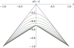
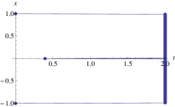
Figure 1. $\sigma=1$, $\mu=\delta_{0}$ and $\nu=\frac{1}{4}\delta_{-1}+\frac{1}{2}\delta_{0}+\frac{1}{4}\delta_{1}$. Above finite difference scheme is used with $\operatorname{CFL}=0.2$ and $50.10^{3}$ time steps on the time domain $\left[0,2\right]$ and spatial domain $\left[-1,1\right]$. The left plot shows that for $t_{0}\sim 0.39$ the potentials touch at $x=0$ which determines the spike of the Root barrier depicted in the right plot.

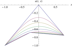
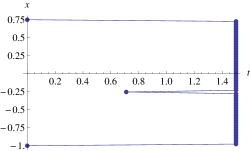
Figure 2. $\sigma=1$,$\mu=\delta_{0}$ and $\nu=\frac{2}{7}\delta_{-1}+\frac{1}{4}\delta_{-\frac{1}{4}}+\frac{13}{28}\delta_{\frac{3}{4}}$.

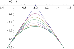
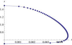
Figure 3. $\sigma\left(x\right)=x$, $\mu=\delta_{1}$ and $\nu=\mathcal{U}\left(\left[\frac{1}{2},\frac{3}{2}\right]\right)$. Initial and target measure are symmetric but the barrier is asymmetric due to $\sigma\left(x\right)=x$.

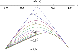
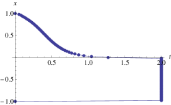
Figure 4. $\sigma\left(x\right)=1$,$\mu=\frac{3}{4}\delta_{-\frac{1}{6}}+\frac{1}{4}\delta_{0.5}$ and $\nu=\frac{1}{3}\delta_{-1}+\frac{2}{3}\mathcal{U}\left(\left[0,1\right]\right).$

4.2. $\mu$ and $\nu$ of unbounded support

For simplicity we restrict ourselves to embeddings into Brownian motion (i.e. $\sigma\equiv 1$). In this case recent results of Jakobsen [33] apply and give a convergence rate of order $\frac{1}{2}$. Denote $h=\left(\Delta t,\Delta x\right)$ and consider schemes of the type

$$u^{h}\left(t+\Delta t,x\right)=\max\left\{u_{\nu}\left(x\right),S_{\Delta t}u^{h}\left(t,x\right)\right\}$$

where $S_{\Delta t}$ is the (formal) solution operator associated to the heat equation $\partial_{t}w-\frac{1}{2}\Delta w=0$. In the case that we use a finite difference method this scheme can be written as

(32) $$\min\left\{u^{h}\left(t+\Delta t,x\right)-u_{\nu}\left(x\right),\frac{u^{h}\left(t+\Delta t,x\right)-u^{h}\left(t,x\right)}{\Delta t}-\frac{u^{h}\left(t,x+\Delta x\right)-2u^{h}\left(t,x\right)+u^{h}\left(t,x-\Delta x\right)}{2\left(\Delta x\right)^{2}}\right\}=0.$$

A direct calculation also shows that this is equivalent to (see Jakobsen [33, page 11 in Section 3])

$$u^{h}\left(t+\Delta t,x\right)=\max\left\{u_{\nu}\left(x\right),u^{h}\left(t,x\right)+\frac{\Delta t}{2\left(\Delta x\right){}^{2}}\left(u^{h}\left(t,x+\Delta x\right)-2u^{h}\left(t,x\right)+u^{h}\left(t,x-\Delta x\right)\right)\right\}$$

and above representation is advantageous for the proof.

Proposition 2 ([33, Section 3]).

Let $\left(1,\mu,\nu\right)$ fulfill Assumption (1). Then there exists a unique $u^{h}$ solving (32). Further, if $\Delta t\leq\left(\Delta x\right)^{2}$ and $u_{0}^{h}$ is an approximation of $u_{0}$ which is bounded independently of $h$ then

$$\left|u-u^{h}\right|_{\infty}\lesssim\sup_{\left[0,\Delta t\right)\times\mathbb{R}}\left|u-u_{0}^{h}\right|+\left(\Delta x\right)^{1/2}$$

Proof.

This is a direct consequence of [33, Section 3] which shows that one can replace the Barles–Souganidis assumptions by more special conditions ($C1-C5$ in [33, Section 2]). A direct calculation shows then that these are fulfilled for the finite-difference scheme under our assumptions. ∎

5. a comparison for obstacle pdes and a lemma about jets

Comparison theorems for obstacle problems can be found in the literature, see [34, 33, 23]. However, due to the unboundedness of the coefficients as well as space they do not cover our setup. We provide a complete proof by revisiting work of [34, 33, 20]. It also establishes Hölder regularity in space of viscosity solutions.

5.1. A Comparison Theorem for the obstacle problem

Theorem 5.

Let $h\in C\left(\mathbb{R},\mathbb{R}\right)$ be of linear growth, i.e.  $\exists c>0$ such that

$$\left|h\left(x\right)\right|\leq c\left(1+\left|x\right|\right)\text{ for all }x\in\mathbb{R}$$

and $\sigma\in C\left(\left[0,T\right]\times\mathbb{R},\mathbb{R}\right)$ Lipschitz in space, uniformly in time ($\sup_{t}\left|\sigma\left(t,.\right)\right|_{Lip}<\infty$). Define

$$F_{obs}\left(t,x,r,a,p,M\right)=\min\left(r-h\left(x\right),a-\frac{\sigma^{2}\left(t,x\right)}{2}m\right).$$

Let $u\in USC\left(\left[0,T\right]\times\mathbb{R},\mathbb{R}\right)$ be a viscosity subsolution and $v\in LSC\left(\left[0,T\right]\times\mathbb{R},\mathbb{R}\right)$ a viscosity supersolution of the PDE

$$F_{obs}\left(t,x,u,\partial_{t}u,Du,D^{2}u\right)\leq 0\leq F_{obs}\left(t,x,v,\partial_{t}v,Dv,D^{2}v\right)\text{ on }\left(0,T\right)\times\mathbb{R}$$

Further assume that $\forall\left(t,x\right)\in\left[0,T\right)\times\mathbb{R}$, $u\left(t,x\right),-v\left(t,x\right)\leq C\left(1+\left|x\right|\right)$ for some constant $C>0$ and that $u\left(0,.\right)$ and $v\left(0,.\right)$ are $\delta$-Hölder continuous. Then there exists a constant $c\geq 0$ s.t. $\forall\left(t,x,y\right)\in\left[0,T\right)\times\mathbb{R}\times\mathbb{R}$

$$u\left(t,x\right)-v\left(t,y\right)\leq\sup_{z\in\mathbb{R}}\left(u_{0}\left(z\right)-v_{0}\left(z\right)\right)+c\inf_{\alpha>0}\left\{\alpha^{-\frac{1}{2-\delta}}+\alpha\left|x-y\right|^{2}\right\}.$$

Direct consequences of this estimate are

1. $u_{0}\leq v_{0}$ implies $u\leq v$ on $\left[0,T\right)\times\mathbb{R}$,

2. if $u$ is also a supersolution (viz. $u$ is a viscosity solution) then $u$ is $\delta$-Hölder continuous in space uniformly in time on $\left[0,T\right)$, i.e.

   $$\sup_{t\in\left[0,T\right)}\left|u\left(t,.\right)\right|_{C^{\delta}\left(\mathbb{R}\right)}<\infty.$$

Proof.

Wlog we can replace the parabolic part in $F$ with $\partial_{t}w-\sigma^{2}\Delta w-w$ (by replacing $u$ resp. $v$ with $e^{-t}u$ resp. $e^{-t}v$). Further we can assume that $\forall\overline{\epsilon}>0$, $u$ is a subsolution of

(33) $$F_{obs}\left(t,x,u,\partial_{t}u,Du,D^{2}u\right) \leq -\frac{\overline{\epsilon}}{\left(T-t\right)^{2}}$$

$$\lim_{t\uparrow T}u\left(t,x\right) = -\infty\text{ uniformly on }\mathcal{O}$$

(by replacing $u$ with $u-\frac{\overline{\epsilon}}{T-t}$). Define for $\alpha>0$,$\epsilon>0$

$$\psi\left(t,x,y\right)=u-v-\phi\left(t,x,y\right)\text{ with }\phi\left(t,x,y\right)=e^{\lambda t}\alpha\left|x-y\right|^{2}+\epsilon\left(\left|x\right|^{2}+\left|y\right|^{2}\right)$$

and

$$m_{\alpha,\epsilon}^{0}=\sup_{\mathbb{R}\times\mathbb{R}}\psi\left(0,x,y\right)^{+}\text{ and }m_{\alpha,\epsilon}=\sup_{\left[0,T\right]\times\mathbb{R}\times\mathbb{R}}\psi\left(t,x,y\right)-m_{\alpha,\epsilon}^{0}.$$

The growth assumptions on $u$ and $v$ together with (33) guarantee for every $\alpha>0$, $\epsilon>0$ the existence of a triple $\left(\hat{t},\hat{x},\hat{y}\right)\in\left[0,T\right)\times\mathbb{R}\times\mathbb{R}$ s.t.

$$m_{\alpha,\epsilon}+m_{\alpha,\epsilon}^{0}=\psi\left(\hat{t},\hat{x},\hat{y}\right).$$

The proof strategy is classic: the above implies that $\forall\alpha>0,\epsilon>0$ and $\forall\left(t,x,y\right)$

(34) $$u\left(t,x\right)-v\left(t,y\right)\leq m_{\alpha,\epsilon}+m_{\alpha,\epsilon}^{0}+e^{\lambda t}\alpha\left|x-y\right|^{2}+\epsilon\left(\left|x\right|^{2}+\left|y\right|^{2}\right).$$

Using the Hölder continuity of $u_{0}$ and $v_{0}$ we immediately get an upper bound for $m_{\alpha,\epsilon}^{0}$

$$m_{\alpha,\epsilon}^{0} \leq u_{0}\left(\hat{x}\right)-v_{0}\left(\hat{x}\right)+\left|v_{0}\right|_{\delta}\left|\hat{x}-\hat{y}\right|^{\delta}-\alpha\left|\hat{x}-\hat{y}\right|^{2}$$

$$\leq \left|u_{0}-v_{0}\right|+c\alpha^{-\frac{1}{2-\delta}}$$

and below we use the parabolic theorem of sums to show that

(35) $$m_{\alpha,\epsilon}\leq C\alpha^{-\frac{1}{2-\delta}}+k\epsilon+\omega_{a}\left(\epsilon\right)$$

where $\omega_{\alpha}\left(.\right)$ is a modulus of continuity for every $\alpha>0$. Plugging these two estimates into (34) gives

$$u\left(t,x\right)-v\left(t,y\right) \leq \left|u_{0}-v_{0}\right|+\left(c+C\right)\alpha^{-\frac{1}{2-\delta}}+e^{\lambda t}\alpha\left|x-y\right|^{2}+\epsilon\left(\left|x\right|^{2}+\left|y\right|^{2}\right).$$

Now letting $\epsilon\rightarrow 0$ and subsequently optimizing over $\alpha$ yields the key estimate

$$u\left(t,x\right)-v\left(t,y\right) \leq \left|u_{0}-v_{0}\right|+\inf_{\alpha>0}\left(\left(c+C\right)\alpha^{\frac{-1}{2-\delta}}+e^{\lambda t}\alpha\left|x-y\right|^{2}\right).$$

Applying it with $x=y$ gives point ((i)) of our statement. Applying it with a viscosity solution $u=v$ gives

$$u\left(t,x\right)-u\left(t,y\right)\leq\inf_{\alpha>0}\left(\left(c+C\right)\alpha^{\frac{-1}{2-\delta}}+e^{\lambda t}\alpha\left|x-y\right|^{2}\right)$$

and the estimate $\inf_{\alpha>0}\left\{\alpha^{-\frac{1}{2-\delta}}+\alpha r^{2}\right\}=cr^{\delta}$ yields the $\delta$-Hölder regularity.

It remains to show (35). Below we assume $m_{\alpha,\epsilon}\geq 0$ and derive the upper bound (35) (which then also holds if $m_{\alpha,\epsilon}<0$). Note that $m_{\alpha,\epsilon}\geq 0$ implies $\hat{t}>0$. The parabolic Theorem of sums [18, Theorem 8.3] shows existence of

$$\left(a,D_{x}\psi\left(\hat{t},\hat{x},\hat{y}\right),X\right)\in\mathcal{\overline{P}}_{\mathcal{O}}^{2,+}u\left(\hat{t},\hat{x}\right)\text{ and }\left(b,D_{y}\psi\left(\hat{t},\hat{x},\hat{y}\right),Y\right)\in\overline{\mathcal{P}}_{\mathcal{O}}^{2,-}v\left(\hat{t},\hat{x}\right)$$

such that

(36) $$a-b=\dot{\psi}\left(\hat{t},\hat{x},\hat{y}\right)\text{ and }\left(\begin{array}[]{cc}X&0\\ 0&-Y\end{array}\right)\leq ke^{\lambda t}\alpha\left(\begin{array}[]{cc}1&-1\\ -1&1\end{array}\right)+k\epsilon\left(\begin{array}[]{cc}1&0\\ 0&1\end{array}\right).$$

Since $u$ is a subsolution resp. $v$ is a supersolution

$$\min\left(a-\frac{\sigma^{2}\left(\hat{t},\hat{x}\right)}{2}X-u\left(\hat{t},\hat{x}\right),u\left(\hat{t},\hat{x}\right)-h\left(\hat{x}\right)\right) \leq 0$$

$$\min\left(b-\frac{\sigma^{2}\left(\hat{t},\hat{y}\right)}{2}Y-v\left(\hat{t},\hat{x}\right),v\left(\hat{t},\hat{x}\right)-h\left(\hat{x}\right)\right) \geq 0$$

and subtracting the second inequality from the first leads to

$$\min\left(a-b-\frac{\sigma^{2}\left(t,x\right)}{2}X+\frac{\sigma\left(\hat{t},\hat{y}\right)}{2}Y-u\left(\hat{t},\hat{x}\right)+v\left(\hat{t},\hat{y}\right),u\left(\hat{t},\hat{x}\right)-v\left(\hat{t},\hat{y}\right)-h\left(\hat{x}\right)+h\left(\hat{y}\right)\right)\leq 0.$$

First assume the second term in the $\min$ is less than or equal to $0$. This gives

$$u\left(\hat{t},\hat{x}\right)-v\left(\hat{t},\hat{y}\right)\leq h\left(\hat{x}\right)-h\left(\hat{y}\right)\leq\left|h\right|_{\delta}\left|\hat{x}-\hat{y}\right|^{\delta}$$

hence we get the estimate

(37) $$m_{\alpha,\epsilon}\leq\left|h\right|_{\delta}\left|\hat{x}-\hat{y}\right|^{\delta}.$$

Now assume the first term in the $\min$ is less than or equal to $0$. This gives

$$\dot{\psi}\left(\hat{t},\hat{x},\hat{y}\right)+u\left(\hat{t},\hat{x}\right)-v\left(\hat{t},\hat{y}\right)\leq\frac{\sigma^{2}\left(t,x\right)}{2}X-\frac{\sigma\left(\hat{t},\hat{y}\right)}{2}Y$$

hence from the definition of $\psi$ resp. $m_{\alpha,\epsilon}$ it then follows that

$$\lambda e^{\lambda t}\alpha\left|\hat{x}-\hat{y}\right|^{2}+m_{\alpha,\epsilon}\leq\frac{1}{2}\left(\sigma^{2}\left(\hat{t},\hat{x}\right)X-\sigma^{2}\left(\hat{t},\hat{y}\right)Y\right).$$

Estimate the rhs by multiplying the matrix inequality (36) from the left respectively right with the vector $\left(\sigma\left(\hat{t},\hat{x}\right),\sigma\left(\hat{t},\hat{y}\right)\right)$ resp. $\left(\sigma\left(\hat{t},\hat{x}\right),\sigma\left(\hat{t},\hat{y}\right)\right)^{t}$ to get

(38) $$\lambda e^{\lambda t}\alpha\left|\hat{x}-\hat{y}\right|^{2}+m_{\alpha,\epsilon} \leq ke^{\lambda t}\alpha\left|\sigma\left(\hat{t},\hat{x}\right)-\sigma\left(\hat{t},\hat{y}\right)\right|^{2}+k\epsilon\left(\sigma^{2}\left(\hat{t},\hat{x}\right)+\sigma^{2}\left(\hat{t},\hat{y}\right)\right)$$

$$\leq ke^{\lambda t}\alpha\left|\sigma\right|_{1}\left|\hat{x}-\hat{y}\right|^{2}+k\epsilon\left(\sigma^{2}\left(\hat{t},\hat{x}\right)+\sigma^{2}\left(\hat{t},\hat{y}\right)\right).$$

By adding (37) and (38) together and choosing $\lambda=\left|\sigma\right|_{1}k+1$ we finally get

$$m_{\alpha,\epsilon}\leq\left|h\right|_{\delta}\left|\hat{x}-\hat{y}\right|^{\delta}-e^{\lambda t}\alpha\left|\hat{x}-\hat{y}\right|^{2}+k\epsilon\left(\sigma^{2}\left(\hat{t},\hat{x}\right)+\sigma^{2}\left(\hat{t},\hat{y}\right)\right).$$

We estimate the sum of the first two terms on the rhs by using that $\sup_{r\geq 0}\left(r^{\delta}+\frac{\alpha}{2}r^{2}\right)\leq c\alpha^{-\frac{1}{2-\delta}}$ and the last term using linear growth of $\sigma^{2}$ to arrive at

$$m_{\alpha,\epsilon}\leq C\alpha^{-\frac{1}{2-\delta}}+k\epsilon\left(1+\left|\hat{x}\right|^{2}+\left|\hat{y}\right|^{2}\right).$$

By lemma (3) we can replace $\epsilon\left(\left|\hat{x}\right|^{2}+\left|\hat{y}\right|^{2}\right)$ by a modulus $\omega_{\alpha}\left(\epsilon\right)$ (i.e. for every $\alpha>0$, $\omega_{\alpha}\in C\left(\left[0,\infty\right),\left[0,\infty\right)\right)$, $\omega_{\alpha}\left(0\right)=0$ and $\omega_{\alpha}$ is non-decreasing), i.e.

$$m_{\alpha,\epsilon}\leq C\alpha^{-\frac{1}{2-\delta}}+k\epsilon+\omega_{a}\left(\epsilon\right).$$

Hence we have shown that $\forall\alpha>0$

$$\limsup_{\epsilon}m_{\alpha,\epsilon}=C\alpha^{-\frac{1}{2-\delta}},$$

and

$$u\left(t,x\right)-v\left(t,y\right)\leq m_{\alpha,\epsilon}+m_{\alpha,\epsilon}^{0}+e^{\lambda t}\frac{\alpha}{2}\left|\hat{x}-\hat{y}\right|^{2}+\epsilon\left(\left|\hat{x}\right|^{2}+\left|\hat{y}\right|^{2}\right).$$

∎

Lemma 3.

Let $f\in USC\left(\left[0,T\right]\times\mathbb{R}\times\mathbb{R}\right)$ and bounded from above. Set

$$m := \sup_{\left[0,T\right]\times\mathbb{R}\times\mathbb{R}}f\left(t,x,y\right)$$

$$m_{\epsilon} := \sup_{\left[0,T\right]\times\mathbb{R}\times\mathbb{R}}f\left(t,x,y\right)-\epsilon\left(\left|x\right|^{2}+\left|y\right|^{2}\right)\text{ for }\epsilon>0.$$

Denote with $\left(\hat{t}_{\epsilon},\hat{x}_{\epsilon},\hat{y}_{\epsilon}\right)$ points where the $sup$ is attained. Then

1. $\lim_{\epsilon\rightarrow 0}m_{\epsilon}=\sup_{\left[0,T\right]\times\mathbb{R}\times\mathbb{R}}f\left(t,x,y\right)$,

2. $\epsilon\left(\left|\hat{x}_{\epsilon}\right|^{2}+\left|\hat{y}_{\epsilon}\right|^{2}\right)\rightarrow_{\epsilon}0$.

Proof.

By definition of a supremum there exists for every $\eta>0$ a triple $\left(t_{\eta},x_{\eta},y_{\eta}\right)\in\left[0,T\right]\times\mathbb{R}\times\mathbb{R}$ such that $f\left(t_{\eta},x_{\eta},y_{\eta}\right)>m-\eta$. Fix $\eta>0$ and take $\epsilon^{\prime}$ small enough s.t. $\epsilon^{\prime}\left(\left|x_{\eta}\right|^{2}+\left|y_{\eta}\right|^{2}\right)\leq\eta$. Then $\forall\epsilon\in\left[0,\epsilon^{\prime}\right]$ we have

$$m\geq m_{\epsilon}\geq f\left(t_{\eta},x_{\eta},y_{\eta}\right)-\epsilon^{\prime}\left(\left|x_{\eta}\right|^{2}+\left|y_{\eta}\right|^{2}\right)\geq f\left(t_{\eta},x_{\eta},y_{\eta}\right)-\eta\geq m-2\eta.$$

Since $\eta$ can be arbitrary small and $\epsilon\mapsto m_{\epsilon}$ is non-increasing the first claim follows. From the above estimate and the boundedness of $f$ from above also show that

$$k_{\epsilon}=\epsilon\left(\left|\hat{x}_{\epsilon}\right|^{2}+\left|\hat{y}_{\epsilon}\right|^{2}\right)$$

is bounded. Hence there exists a subsequence of $\left(k_{\epsilon}\right)_{\epsilon>0}$ which we denote with slight abuse of notation again as $\left(k_{\epsilon}\right)_{\epsilon>0}$ which converges to some limit denoted $k$($\geq 0$). Now

$$f\left(\hat{t}_{\epsilon},\hat{x}_{\epsilon},\hat{y}_{\epsilon}\right)-k_{\epsilon}\leq m-k_{\epsilon}$$

and from the first part we can send $\epsilon$ to $0$ along the subsequence and see that $m-k\leq m$, hence $k=0$. Since we have shown that every subsequence $\left(k_{\epsilon}\right)$ converges to $0$ the second statement follows. ∎

5.2. A Lemma about sup- and superjets

We now provide the proof of the Lemma that plays a crucial role in the proof of Theorem (2). It describes the elements in the sub and superjets $\mathcal{P}_{\mathcal{O}}^{2,-}\left(u\right)$ and $\mathcal{P}_{\mathcal{O}}^{2,+}\left(u\right)$ for functions which are only left- and right-differentiable.

Lemma 4.

Let $v\in C\left(\left(0,\infty\right)\times\mathbb{R},\mathbb{R}\right)$ and assume that $\forall\left(t,x\right)\mathbb{\in}\left(0,\infty\right)\times\mathbb{R}$, $v$ has a left- and right-derivative, i.e. the following limits exist

$$\partial_{t+}v\left(t,x\right)=\lim_{\epsilon\searrow 0}\frac{v\left(t+\epsilon,x\right)-v\left(t,x\right)}{\epsilon}\text{ and }\partial_{t-}v\left(t,x\right)=\lim_{\epsilon\nearrow 0}\frac{v\left(t+\epsilon,x\right)-v\left(t,x\right)}{\epsilon},$$

If $\partial_{t-}v\left(t,x\right)\leq\partial_{t+}v\left(t,x\right)$ then

$$a\in\left[\partial_{t-}v\left(t,x\right),\partial_{t+}v\left(t,x\right)\right]\,\,\,\forall\left(a,p,m\right)\in\mathcal{P}_{\mathcal{O}}^{2,-}v\left(t,x\right).$$

If $\partial_{t-}v\left(t,x\right)<\partial_{t+}v\left(t,x\right)$ then $\mathcal{P}_{\mathcal{O}}^{2,+}v\left(t,x\right)=\emptyset$ and if $\partial_{t-}v\left(t,x\right)=\partial_{t+}v\left(t,x\right)$ then $\forall\left(a,p,m\right)\in\mathcal{P}_{\mathcal{O}}^{2,+}v\left(t,x\right)$, $a=\partial_{t}v\left(t,x\right)$ ($=\partial_{t-}v\left(t,x\right)=\partial_{t+}v\left(t,x\right)$). In all the above cases, if $v$ is additionally twice continuously differentiable in space then

$$m \leq \Delta v\left(t,x\right)\,\,\,\forall\left(a,p,m\right)\in\mathcal{P}_{\mathcal{O}}^{2,-}v\left(t,x\right),$$

$$m \geq \Delta v\left(t,x\right)\,\,\,\forall\left(a,p,m\right)\in\mathcal{P}_{\mathcal{O}}^{2,+}v\left(t,x\right).$$

Proof.

Every element $\left(a,p,m\right)\in\mathcal{P}_{\mathcal{O}}^{2,-}v\left(t,x\right)$ fulfills

$$v\left(t+\epsilon,x\right)-v\left(t,x\right)\geq a\epsilon+o\left(\epsilon\right)\,\,\,\epsilon\rightarrow 0.$$

Applied with a sequence $\epsilon^{n}\nearrow 0,$ it follows after dividing by $\epsilon^{n}$ and letting $n\rightarrow\infty$ that $\partial_{t-}v\left(t,x\right)\leq a$. If $\partial_{t-}v\left(t,x\right)<\partial_{t+}v\left(t,x\right)$ then for $\left(a,p,m\right)\in\mathcal{P}_{\mathcal{O}}^{2,+}v\left(t,x\right)$ we have

$$v\left(t+\epsilon,x\right)-v\left(t,x\right)\leq a\epsilon+o\left(\epsilon\right)\,\,\,\epsilon\rightarrow 0$$

which leads after taking $\epsilon^{n}\nearrow 0$ resp. $\epsilon^{n}\searrow 0$ to

$$\partial_{t+}v\left(t,x\right)\leq a\leq\partial_{t-}v\left(t,x\right)$$

and hence contradicts the assumption $\partial_{t-}v\left(t,x\right)<\partial_{t+}v\left(t,x\right)$. The other statements follow similarly.∎

Acknowledgement 1.

PG is grateful for partial support from the European Research Council under the European Union’s Seventh Framework Programme (FP7/2007–2013)/ERC grant agreement nr. 258237. and nr. 291244. HO is grateful for partial support from the European Research Council under the European Union’s Seventh Framework Programme (FP7/2007–2013)/ERC grant agreements nr. 258237 and nr. 291244. GdR is also affiliated with CMA/FCT/UNL, 2829-516 Caparica, Portugal. GdR acknowledges partial support by the Fundação para a Ciência e a Tecnologia (Portuguese Foundation for Science and Technology) through PEst-OE/MAT/UI0297/2011 and PEst-OE/MAT/UI0297/2014 (CMA - Centro de Matemática e Aplicações).

Acknowledgement 2.

The authors would like to thank Alexander Cox, Martin Keller–Ressel, Jan Obłój and Johannes Ruf for helpful conversations.

References

- [1] S. Ankirchner, D. Hobson, and P. Strack. Finite, integrable and bounded time embeddings for diffusions. ArXiv e-prints, June 2013.
- [2] Stefan Ankirchner, Gregor Heyne, and Peter Imkeller. A BSDE approach to the Skorokhod embedding problem for the Brownian motion with drift. Stoch. Dyn., 8(1):35–46, 2008.
- [3] Stefan Ankirchner and Philipp Strack. Skorokhod embeddings in bounded time. Stochastics and Dynamics, 11(02n03):215–226, 2011.
- [4] G. Barles, Ch. Daher, and M. Romano. Convergence of numerical schemes for parabolic equations arising in finance theory. Math. Models Methods Appl. Sci., 5(1):125–143, 1995.
- [5] G. Barles and P. E. Souganidis. Convergence of approximation schemes for fully nonlinear second order equations. Asymptotic Anal., 4(3):271–283, 1991.
- [6] G. Barles and P.E. Souganidis. Convergence of approximation schemes for fully nonlinear second order equations. In Decision and Control, 1990., Proceedings of the 29th IEEE Conference on, pages 2347 –2349 vol.4, dec 1990.
- [7] Guy Barles. A new stability result for viscosity solutions of nonlinear parabolic equations with weak convergence in time. C. R. Math. Acad. Sci. Paris, 343(3):173–178, 2006.
- [8] M. Beiglböck and N. Juillet. On a problem of optimal transport under marginal martingale constraints. arXiv 1208.1509, August 2012.
- [9] Mathias Beiglböck and Martin Huesmann. Optimal transport and skorokhod embedding. arXiv preprint arXiv:1307.3656, 2013.
- [10] A. Bensoussan and J.L. Lions. Applications of variational inequalities in stochastic control, volume 12. North Holland, 1982.
- [11] R. Buckdahn, J. Huang, and J. Li. Regularity properties for general HJB equations: a backward stochastic differential equation method. SIAM J. Control Optim., 50(3):1466–1501, 2012.
- [12] R. Chacon and J. Walsh. One-dimensional potential embedding. Séminaire de Probabilités X Université de Strasbourg, pages 19–23, 1976.
- [13] R. V. Chacon. Potential processes. Trans. Amer. Math. Soc., 226:39–58, 1977.
- [14] Rene Chacon. Barrier stopping times and the filling scheme. PhD Dissertation, University of Washington, 1985.
- [15] A. M. G. Cox and J. Wang. Optimal robust bounds for variance options. ArXiv e-prints, August 2013.
- [16] Alexander M. G. Cox and Jiajie Wang. Root’s barrier: Construction, optimality and applications to variance options. The Annals of Applied Probability, 23(3):859–894, 06 2013.
- [17] AMG Cox and G Peskir. Embedding laws in diffusions by functions of time. arXiv preprint arXiv:1201.5321, 2012.
- [18] M. G. Crandall, H. Ishii, and P.-L. Lions. User’s guide to viscosity solutions of second order partial differential equations. Bull. Amer. Math. Soc. (N.S.), 27(1):1–67, 1992.
- [19] Michael G. Crandall, Hitoshi Ishii, and Pierre-Louis Lions. User’s guide to viscosity solutions of second order partial differential equations. Bull. Amer. Math. Soc. (N.S.), 27(1):1–67, 1992.
- [20] J. Diehl, P. Friz, and H. Oberhauser. Parabolic comparison revisited and applications. 2014. In press.
- [21] Hermann Dinges. Stopping sequences. In Séminaire de Probabilités VIII Université de Strasbourg, pages 27–36. Springer, 1974.
- [22] B. Dupire. Arbitrage bounds for volatility derivatives as free boundary problem. Presentation at PDE and Mathematical Finance, KTH, Stockholm, 2005.
- [23] N. El Karoui, C. Kapoudjian, E. Pardoux, S. Peng, and M.C. Quenez. Reflected solutions of backward SDEs, and related obstacle problems for PDEs. the Annals of Probability, 25(2):702–737, 1997.
- [24] N. El Karoui, S. Peng, and M. C. Quenez. Backward stochastic differential equations in finance. Math. Finance, 7(1):1–71, 1997.
- [25] W. H. Fleming and H. M. Soner. Controlled Markov processes and viscosity solutions, volume 25 of Stochastic Modelling and Applied Probability. Springer, New York, second edition, 2006.
- [26] Wendell H. Fleming and H. Mete Soner. Controlled Markov processes and viscosity solutions, volume 25 of Stochastic Modelling and Applied Probability. Springer, New York, second edition, 2006.
- [27] A. Galichon, P. Henry-Labordère, and N. Touzi. A stochastic control approach to no-arbitrage bounds given marginals, with an application to lookback options. The Annals of Applied Probability, 24(1):312–336, 02 2014.
- [28] Paul Gassiat, Aleksandar Mijatovic, and Harald Oberhauser. An integral equation for Root’s barrier and the generation of Brownian increments. Annals of Applied Probability (in press), 2014.
- [29] Pierre Henry-Labordere, Jan Obloj, Peter Spoida, and Nizar Touzi. Maximum maximum of martingales given marginals. arXiv preprint arXiv:1203.6877, 2012.
- [30] F. Hirsch and B. Roynette. A new proof of Kellerer’s theorem. ESAIM: Probability and Statistics, to appear, 2012.
- [31] D. Hobson. The Skorokhod Embedding Problem and Model-Independent Bounds for Option Prices. In Paris-Princeton Lectures on Mathematical Finance 2010, volume 2003 of Lecture Notes in Mathematics, pages 267–318. Springer Berlin / Heidelberg, 2011.
- [32] David G Hobson. Robust hedging of the lookback option. Finance and Stochastics, 2(4):329–347, 1998.
- [33] E.R. Jakobsen. On the rate of convergence of approximation schemes for bellman equations associated with optimal stopping time problems. Mathematical Models and Methods in Applied Sciences, 13(05):613–644, 2003.
- [34] E.R. Jakobsen and K.H. Karlsen. Continuous dependence estimates for viscosity solutions of fully nonlinear degenerate parabolic equations. Journal of Differential Equations, 183(2):497–525, 2002.
- [35] Hans G Kellerer. Markov-komposition und eine Anwendung auf Martingale. Mathematische Annalen, 198(3):99–122, 1972.
- [36] Jack Kiefer. Skorohod embedding of multivariate rv’s, and the sample df. Zeitschrift für Wahrscheinlichkeitstheorie und verwandte Gebiete, 24(1):1–35, 1972.
- [37] Victor Kleptsyn and Aline Kurtzmann. A counter-example to the cantelli conjecture. arXiv preprint arXiv:1202.2250, 2012.
- [38] R. M. Loynes. Stopping times on Brownian motion: Some properties of Root’s construction. Z. Wahrscheinlichkeitstheorie und Verw. Gebiete, 16:211–218, 1970.
- [39] Terry R McConnell. The two-sided stefan problem with a spatially dependent latent heat. Transactions of the American Mathematical Society, 326(2):669–699, 1991.
- [40] D. Nualart. The Malliavin calculus and related topics. Probability and its Applications (New York). Springer-Verlag, Berlin, second edition, 2006.
- [41] Diana Nunziante. Existence and uniqueness of unbounded viscosity solutions of parabolic equations with discontinuous time-dependence. Nonlinear Anal., 18(11):1033–1062, 1992.
- [42] J. Obłój. The Skorokhod embedding problem and its offspring. Probab. Surv., 1:321–390, 2004.
- [43] J. Obłój. On some aspects of Skorokhod embedding problem and its applications in mathematical finance. Notes for the students of the 5th European summer school in financial mathematics, 2012.
- [44] Jan Obłój and Peter Spoida. An iterated Azéma–Yor type embedding for finitely many marginals. arXiv preprint arXiv:1304.0368, 2013.
- [45] D. H. Root. The existence of certain stopping times on Brownian motion. Ann. Math. Statist., 40:715–718, 1969.
- [46] H. Rost. Die Stoppverteilungen eines Markoff-Prozesses mit lokalendlichem Potential. Manuscripta Math., 3:321–329, 1970.
- [47] H. Rost. The stopping distributions of a Markov Process. Invent. Math., 14:1–16, 1971.
- [48] H. Rost. Skorokhod’s theorem for general Markov processes. In Transactions of the Sixth Prague Conference on Information Theory, Statistical Decision Functions, Random Processes (Tech. Univ. Prague, Prague, 1971; dedicated to the memory of Antonín Špaček), pages 755–764. Academia, Prague, 1973.
- [49] H. Rost. Skorokhod stopping times of minimal variance. In Séminaire de Probabilités, X (Première partie, Univ. Strasbourg, Strasbourg, année universitaire 1974/1975), pages 194–208. Lecture Notes in Math., Vol. 511. Springer, Berlin, 1976.