Hybrid methods in planetesimal dynamics:
Formation of protoplanetary systems and the mill condition

Abstract

The formation and evolution of protoplanetary discs remains a challenge from both a theoretical and numerical standpoint. In this work we first perform a series of tests of our new hybrid algorithm presented in Glaschke, Amaro-Seoane and Spurzem 2011 (henceforth Paper I) that combines the advantages of high accuracy of direct-summation $N-$body methods with a statistical description for the planetesimal disc based on Fokker-Planck techniques. We then address the formation of planets, with a focus on the formation of protoplanets out of planetesimals. We find that the evolution of the system is driven by encounters as well as direct collisions and requires a careful modelling of the evolution of the velocity dispersion and the size distribution over a large range of sizes. The simulations show no termination of the protoplanetary accretion due to gap formation, since the distribution of the planetesimals is only subjected to small fluctuations. We also show that these features are weakly correlated with the positions of the protoplanets. The exploration of different impact strengths indicates that fragmentation mainly controls the overall mass loss, which is less pronounced during the early runaway growth. We prove that the fragmentation in combination with the effective removal of collisional fragments by gas drag sets an universal upper limit of the protoplanetary mass as a function of the distance to the host star, which we refer to as the mill condition.

1 Introduction

The origin of our solar system remains to be one of the most exciting problems of today’s astronomy. For a long time it has been the only known planetary system. While it is still the only planetary system that can be studied in detail, progress in observation techniques has led to the discovery of extrasolar planets and even some extrasolar planetary systems. The wealth of observational data raised the question of how a planetary system forms in general. As of writing these lines, 859 planets and 676 planetary systems are known. Most of these planetary systems are very different compared to our solar system.

Understanding planet formation comprises many challenges, such as hydrodynamics of the protoplanetary disc, chemical evolution of the embedded dust grains, migration of planets and planetesimals and even star-star interactions in dense young star clusters (see Armitage 2010, for a review and references therein, and also the introduction of Paper I, for a brief summary). All these components constitute the frame for the essential process of planet formation: An enormous growth from dust-sized particles to the final planets, accompanied by a steady decrease of the number of particles which contain most of the mass over many orders of magnitude. The particle number changes over many orders of magnitude as planetary growth proceeds. There is active research on each of the different aspects of planet formation, but the current efforts are far from a unified model of planet formation (Goldreich et al. 2004; Lissauer 1993).

We address the study of this many–to–few transition from planetesimals to few protoplanets. This stage is of particular interest, as it links the early planetesimal formation to the final planet formation. Collisions still play a major role in the evolution of the system, and the close interplay between the change of the size distribution and the evolution of the random velocities requires a careful treatment of the complete size range.

Small $N-$body simulations (i.e. with less than few $10^{4}$ particles) have been useful in exploring the basic growth mechanisms at the price of a modified timescale and an artificially reduced particle number (e.g. Kokubo 1995, 1996). Statistical codes explored the limit of large particle numbers in the early phases and are now tentatively applied to the full planet formation process. An efficient solution would be the combination of these two approaches in one hybrid code to unify the advantages of both methods.

In this work, we present a series of tests and first results of our new hybrid code, which was presented in Paper I. As described in the first paper, it combines the Nbody6 code (a descendant of the widespread $N-$body family (see Aarseth 1999; Spurzem 1999; Aarseth 2003) with a new statistical code which uses recent works on the statistical description of planetesimal systems. The new hybrid code includes a consistent modelling of the velocity distribution and the mass spectrum over the whole range of relevant sizes, which allows us to apply a detailed collision model rather than the perfect-merger assumption used in previous $N-$body simulations. We then apply this new code to follow the formation of protoplanets out of 1–10 km sized planetesimals. In section 2 we present a series of tests that check for the rubustness of the code. In section 3.1 we explain the initial conditions we use for our numerical experiments, which we show in section 3.2. In section 4 we derive a useful relation that allows us to introduce an universal upper limit of the protoplanetary mass as a function of the distance to the host star. Finally, in section 5 we discuss our progress and results and potential future applications.

2 Validating the Code

The new hybrid code requires the implementation of rather different methods within a single framework. We have here two possible sources of problems. First, the method is new and therefore it must be carefully assessed with other work; on the other hand, the implementation must also be checked meticulously, since it combines two rather different approaches. We hence present in this section a number of tests to check all code components, namely the evolution of the velocity dispersion, the accuracy of the solver of the coagulation equation, the proper joining of statistical and $N-$body component and an overall comparison of statistical, $N-$body and hybrid calculations. Table 1 summarises the selected test runs with the respective initial conditions.

No.	$\Sigma$	$\Delta a$	$N$	$N_{\mathrm{rad}}$	$e^{2}/h^{2}$	$i^{2}/h^{2}$	$m$	Type
T1a	$1.1251\times 10^{-6}$	0.02	1000	–	0.04	0.01	$1.41\times 10^{-10}$	$N-$body
T1b	$1.1251\times 10^{-6}$	0.02	500	10	0.04	0.01	$1.41\times 10^{-10}$	Hybrid
T1c	$1.1251\times 10^{-6}$	0.02	–	10	0.04	0.01	$1.41\times 10^{-10}$	Statistic
T2a	$0.5626\times 10^{-6}$	0.08	800	–	4	1	$5\times 10^{-10}$	$N-$body
	$0.5626\times 10^{-6}$		200	–	4	1	$2\times 10^{-9}$
T2b	$0.5626\times 10^{-6}$	0.08	–	10	4	1	$5\times 10^{-10}$	Hybrid
	$0.5626\times 10^{-6}$		200	–	4	1	$2\times 10^{-9}$
T3	Safronov	–	–	–	–	–	–	Statistic
T4a	$1.1251\times 10^{-6}$	0.02	10.000	–	4	1	$1.41\times 10^{-11}$	$N-$body
T4b	$1.1251\times 10^{-6}$	0.02	–	10	4	1	$1.41\times 10^{-11}$	Hybrid
T4c	$1.1251\times 10^{-6}$	0.02	–	10	4	1	$1.41\times 10^{-11}$	Statistic
T5	$1.8789\times 10^{-6}$	–	–	–	620	155	$2.4\times 10^{-15}$	Statistic

Table 1: Parameters of all test simulations (and hence preceded by a “T”). The transition mass in T4b is $m_{\mathrm{trans}}=3.1\times 10^{-10}$ Only simulations T3, T4a–T4c and T5 include collisions. All values use $M_{c}=G=r_{0}=1$.

2.1 Energy Balance

The first test run is dedicated to a careful check of the interplay between statistical component and $N-$body component with respect to the evolution of the velocity dispersion. We therefore exclude from this first test collisions and accretion.

We use a homogeneous ring of planetesimals as our first test. The reason is that we can analyse the evolution with three different setups – a pure $N-$body calculation, a pure statistical calculation and a mixed hybrid calculation. All three approaches should in principle reproduce the same result. Hence we prepare a small $N-$body test run (T1a) and let the system evolve (see figure 1). As a second test run, we shift one half of the bodies to the statistical model and conduct the integration again (T1b). While this usage of the hybrid code is somewhat artificial, it provides an excellent setup to examine the interplay between $N-$body and statistical part, since neither component dominates the result. Finally, we run a complete statistical calculation (T1c).

Figure 1: Test simulations T1a–T1c (uniform mass, see table 1). We show the results from the $N-$body calculation (100% $N-$body), the statistical calculation (100% Statistic) and the hybrid calculation (50% Statistic refers to the statistical component, whereas 50% $N-$body is the $N-$body part). The red curve is the eccentricity data, and the green curve the inclination.

We can see that all different approaches are in good agreement. Although the accordance between $N-$body and statistical calculation is not a new finding – it merely shows that the stirring terms provide a proper description of a planetesimal system (this was already shown by Ohtsuki et al. (2002)) – we deem the test to be necessary to demonstrate that the agreement holds in our approach and, in particular, that the accuracy in the integration of the statistical model is robust. A more stringent test is posed by the hybrid run, which proves that the pseudo-force method links both code components in a consistent way without spurious energy transfer. In this respect, figure 1 includes both components of the hybrid calculation separately, but the difference is so small that they are hardly distinguishable.

We also run a second test runs that follow the same approach but with a bimodal mass distribution, with the same total mass in both components. The first case, T2a, is a pure $N-$body calculation, whereas the second one treats the smaller particles with the statistical model. This test is particularly interesting because it is close to the real purpose of our hybrid code. In figure 2 we can see that there is a satisfactory agreement between the two test runs.

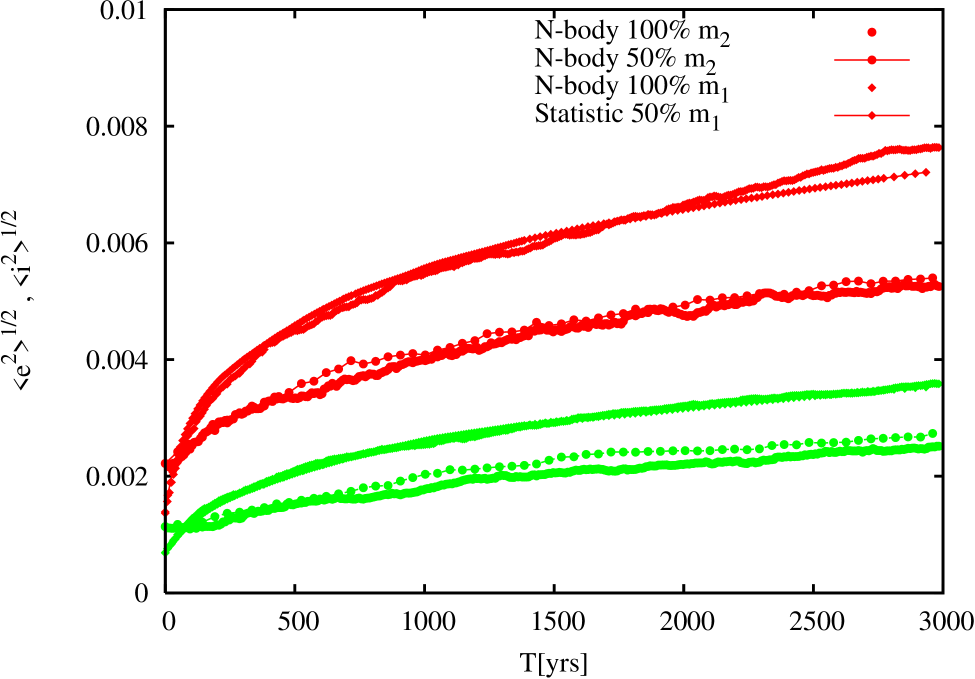
Figure 2: Comparison of the $N-$body calculation T2a with the hybrid calculation T2b. The coding is the same as in figure 1.

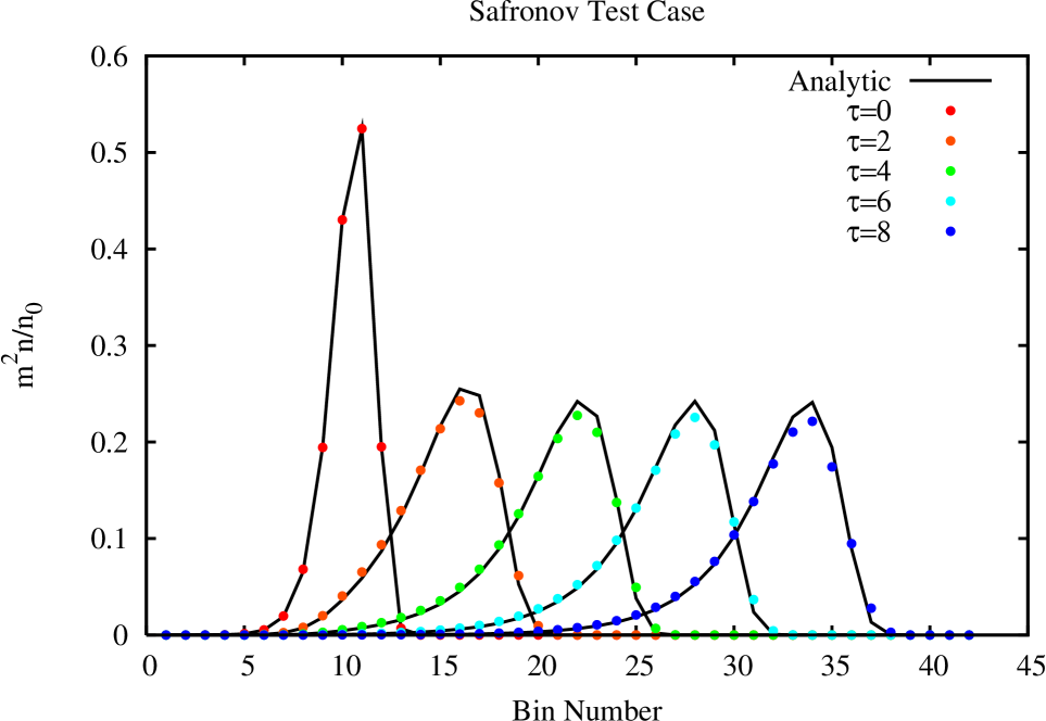
Figure 3: Test of the solution of the coagulation equation (T3). The analytical solution is presented in Paper I.

2.2 Coagulation Equation

In this section we verify the numerical solution of the coagulation equation by running a comparison with the analytic solution of the Safronov problem, as presented in Paper I.

The collisional cross-section is assumed to be proportional to the sum of the masses of the colliding bodies. Thus, the coagulation kernel is known and an additional integration of the velocity dispersions is not necessary. Figure 3 summarises the numerical solution, simulation T3, of the Safronov test.

The mass bins are spaced by a factor $\delta=2$. While some slight differences emerge near the maximum of the density distribution, the overall shape is well conserved throughout the integration. This proves that a spacing within a factor two still guarantees a reliable solution of the coagulation equation without a modified timescale for the growth.

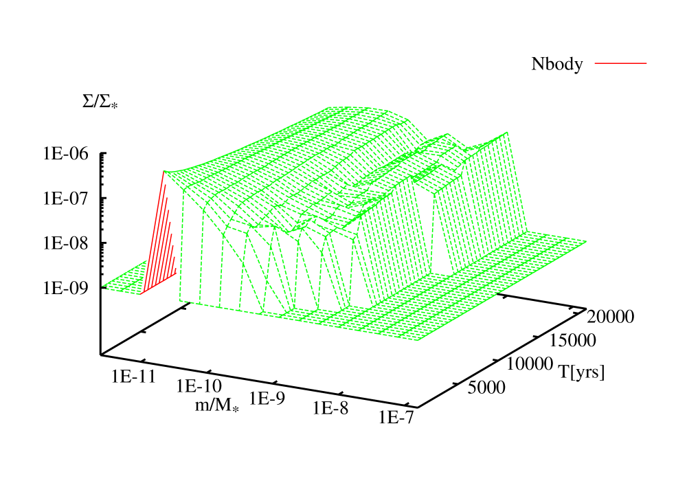
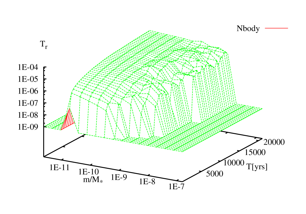
Figure 4: Surface density and radial velocity dispersion of the $N-$body model (T4a).

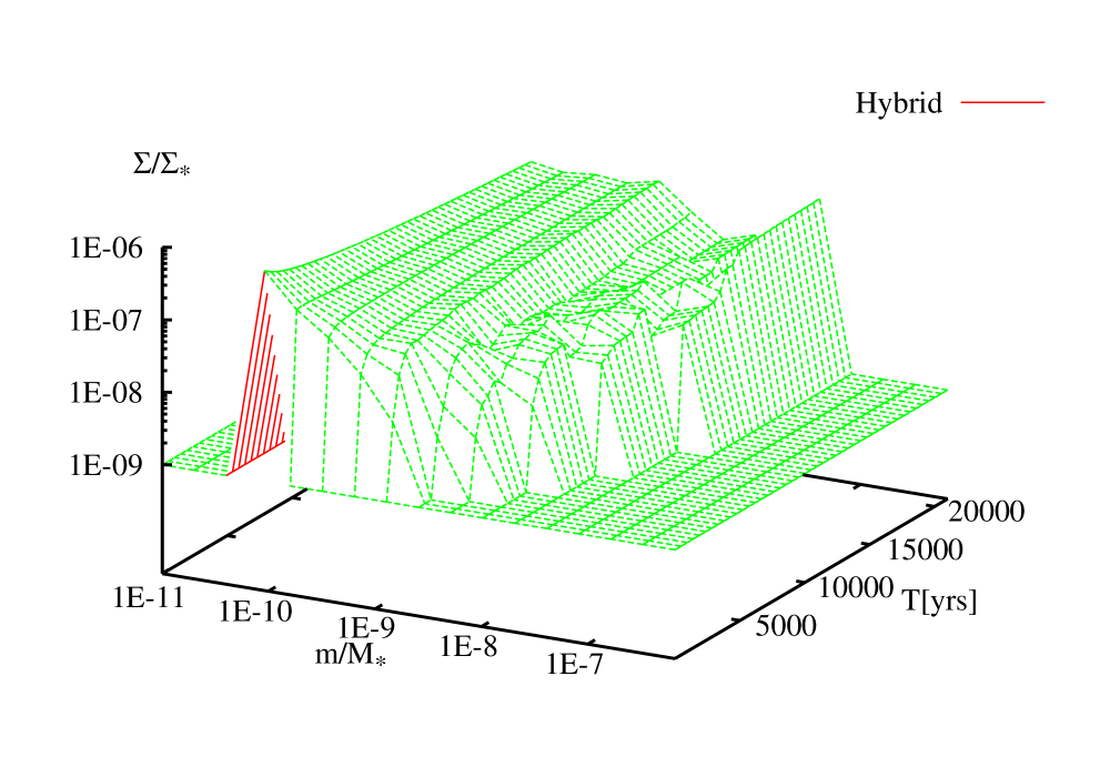
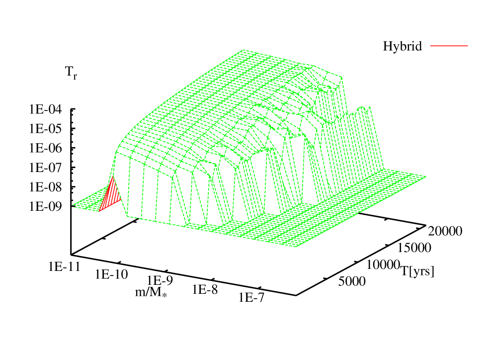
Figure 5: Surface density and radial velocity dispersion of the hybrid model (T4b).

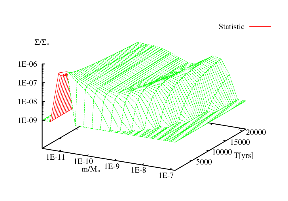
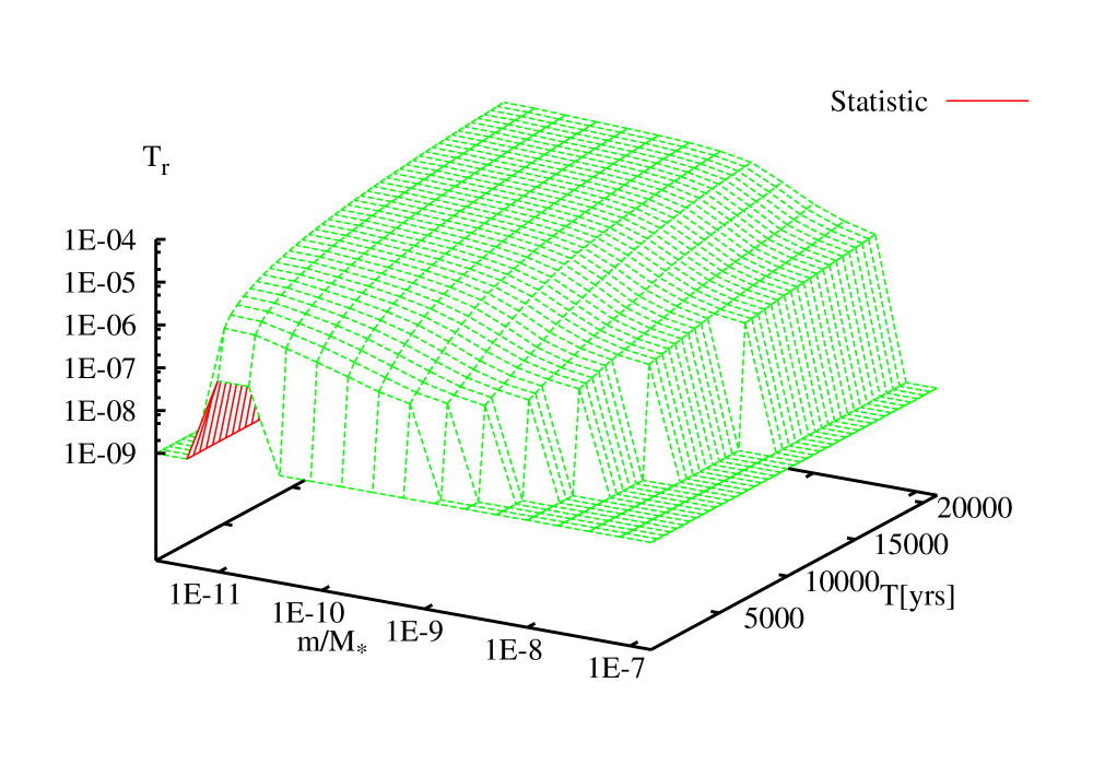
Figure 6: Surface density and radial velocity dispersion of the statistical model (T4c).

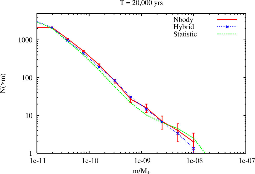
Figure 7: Cumulative size distribution of the comparative runs T4a–T4c at T=20,000 yr.

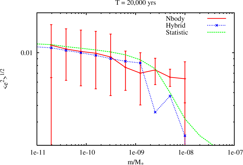
Figure 8: Mean square eccentricities of the comparative runs T4a–T4c at T=20,000 yr. Error bars indicate the spread due to the rayleigh distribution of the eccentricity.

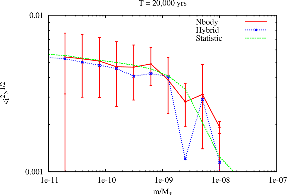
Figure 9: The same as figure 8 for the inclination. The strong deviation at $m=3\times 10^{-9}$ is due to a single particle.

2.3 Testing the complete code

The most robust test of our hybrid code (or the stand-alone statistical code) is a comparison with a pure $N-$body simulation with the same initial conditions. While a large particle number is desirable to cover a large range in masses, we are limited in the number of particles to be used in the direct $N-$body techniques to a few $10^{4}$.

Figure 10: Comparative calculation T5 which adopts the initial conditions of Inaba et al. 2001 (their figure 9, bottom).

We therefore choose a single-mass system with initially 10,000 particles. We enlarge the radii of the planetesimal by a factor $f=5$, which speeds up the calculation without modifying the growth mode. The transition mass is twenty times larger than the initial planetesimal mass, keeping the particle number covered by the statistical component larger than a few thousands.

We compare a full $N-$body run with a hybrid calculation and a pure statistical calculation. Though the stand-alone statistical calculation includes the proper treatment of the runaway bodies via the gravitational range method, if only few particles reside in one mass bin we do not take into account suppression of self-accretion and self-stirring. While the hybrid approach describes this regime in much more detail, we include the full statistical calculation nevertheless for completeness.

In figures 4–6 we have an overview of the time evolution of the system, where all quantities are integrated over the whole system. All calculations seem to agree rather well, although the statistical noise in the $N-$body calculation and the hybrid calculation is quite strong due to the particle number. Runaway growth leads to the fast formation of a few protoplanets on a timescale of a few thousand years, with a good agreement of the fast initial growth phase in all three test runs. The boundary between smooth evolution and noisy data marks the location of the transition mass in the hybrid calculation.

We compare the size distribution and the velocity dispersion at the end of the integration, which is 20,000 yr, in more detail in figures 7–9. Both the $N-$body data and the hybrid data are projected on to the same grid as the full statistical calculation to allow a convenient comparison.

The agreement of the size distribution $N(>m)$ is excellent; the small deviations are within the statistical error. We note that the strong variations in the size distributions of figures 4–6 are located at the high mass end, where only few particles dominate the surface density. In addition, the growth in the statistical model seems to be faster than the $N-$body reference calculation. However, the density at the highest masses refers to less than one particle. As we noted before, this is due to the poor treatment of the few–body limit.

The comparison of the velocity dispersions yields good results, in particular in the low–mass regime, where the statistical error is small. The high mass regime does not only suffer from bad statistics, but also from a pronounced time variability, as we can see by comparing the fluctuations in figures 4–6. Taking these variations into account, all three calculations are in good agreement. As before, the deviation at $m=3\times 10^{-9}$ is due to a single particle.

2.4 The statistical code

Inaba et al. (2001) presented a high accuracy statistical code. In this section we run our last test calculation by comparing with this work, in particular with their figure 9, bottom. They included in their code approximately the same physics and interpolation formulae, with only minor differences to our approach.

While our approach allows us to set a spacing up to $\delta=2$, their solution of the coagulation requires a smaller spacing, of $\delta=1.1$, to guarantee a reliable solution. The few-body limit is handled properly, with an additional treatment of the protoplanets via the gravitational-range approach. In figure 10 we show our comparison, simulation T5, with their runs. Again, we find a good agreement but for minor deviations. These are likely related to the different implementation of the collisional probability.

3 Simulations: Protoplanetary growth

3.1 Initial conditions

We apply our hybrid code now to a well defined initial setup of a planetesimal disc. All simulations use a homogenous ring of planetesimals extending from an inner boundary $R_{\min}$ to an outer boundary $R_{\max}$. Since radial migration is not included, all planetesimals are bounded to this volume throughout the simulation. The central star has a mass of one solar mass. Each simulation starts with no $N-$body particles, so that we need only to specify the setup for the statistical part of the calculation. The differential surface density as a function of mass is

$$\frac{d\Sigma}{dm} =\Sigma_{0}\frac{m}{{\bar{m}}^{2}}\exp\,\left(-m/\bar{m}\right)$$ (1)

$${\rm Var}(m) ={\bar{m}}^{2},$$ (2)

where $\Sigma_{0}$ is the total surface density and $\bar{m}$ is the mean mass. Equation 1 provides a smooth variation over a few mass bins, which avoids numerical problems at the beginning of the simulation. The initial velocity dispersion is related to the mean escape velocity $v_{\infty}$ of the initial size distribution defined by Eq. 1

$$\frac{1}{100}v_{\infty}^{2}=T_{r}+T_{\phi}+T_{z},$$ (3)

with the ratio of the velocity dispersions

$$T_{r}=4T_{\phi}=4T_{z}$$ (4)

We adopt a rather small initial velocity dispersion to avoid strong spurious fragmentation due to an overestimation of the velocity dispersion. Furthermore, strong relaxation in the initial phase of the calculation quickly establishes an equilibrium velocity dispersion. The time step control parameters are chosen such that the energy error $\Delta E/E$ of the $N-$body component remains always smaller than $10^{-8}$ throughout the simulation. Likewise, our choice of the parameters of the statistical component assures that the statistical model is solved accurately and remains stable, as indicated by the set of comparative runs. All runs simulate only a narrow ring centred at a distance $r_{c}$ and we choose the following units:

$$r_{c}=1\qquad M_{c}=1\qquad G=1$$ (5)

In table 2 we summarise the main parameters of the simulations, fixed to the same values for all of them.

3.2 Main objectives of the analysis

The scheme we have developed is in principle ready to solve the complete planetesimal problem, at least concerning the large range of sizes. However, in practise we are limited by the computational power. A small ring with a width of 0.1 AU centred at 1 AU with a moderate size for the lower cut-off requires some days of integration, with the largest fraction of time spent in the statistical model. While we focus on these initial conditions for our simulations, we also present some more refined models that required larger calculations. We adapt a surface density $\Sigma=10$ g/cm² in the simulations, which can be envisaged as a nominal value used in the related literature. In the remaining of this work, we focus on the following aspects of protoplanetary growth:

$\eta_{\mathrm{Disc}}$	0.01
$\eta_{\mathrm{reg}}$	0.002
$\eta_{\mathrm{irr}}$	0.001
$R_{\min}$	0.95	AU
$R_{\max}$	1.05	AU
$\bar{m}$	$3\times 10^{18}$	g
$\rho$	2.7	g/cm3
$\delta$	2
$\Delta v_{g}$	60	m/s

Table 2: General parameters common to all simulations listed in table 3.

Code	Strength	$N_{M}$	$N_{R}$	$\Sigma[$g$/$cm${}^{2}]$	$m_{\min}/M_{c}$	$m_{\mathrm{trans}}/M_{c}$	$\rho_{g}[$g$/$cm${}^{3}]$
S1FB	B&A 1999	24	50	10	$3.48\times 10^{-18}$	$3.89\times 10^{-11}$	$10^{-9}$
S2FH	H&H 1990	24	50	10	$3.48\times 10^{-18}$	$3.89\times 10^{-11}$	$10^{-9}$
S3FN	Perfect Merger	24	50	10	$3.48\times 10^{-18}$	$3.89\times 10^{-11}$	$10^{-9}$
S4FBN	B&A 1999	24	50	10	$3.48\times 10^{-18}$	$3.89\times 10^{-11}$	$0$
S5FBL	B&A 1999	24	5	10	$3.48\times 10^{-18}$	$3.89\times 10^{-11}$	$10^{-9}$
S6FBH	B&A 1999	24	100	10	$3.48\times 10^{-18}$	$3.89\times 10^{-11}$	$10^{-9}$
S7FB2	B&A 1999	40	50	10	$5.31\times 10^{-23}$	$3.89\times 10^{-11}$	$10^{-9}$
S8_S2	B&A 1999	15	50	2	$3.48\times 10^{-18}$	$4.87\times 10^{-12}$	$2\times 10^{-10}$
S9_S100	B&A 1999	27	50	100	$3.48\times 10^{-18}$	$3.11\times 10^{-10}$	$10^{-8}$

Table 3: Complete list of all simulations (the names of the models are therefore preceded with an “S”). The first group examines different collisional models, the second group resumes the nominal simulation S1FB with different resolutions and the third group explores different surface densities.

1. Different collision models: This represents a fundamental uncertainty, since the impact physics of planetesimals is not well established yet. In order to do realistic models of planetesimal collisions we need to understand the internal structure of the bodies taking part in the collision. Planetesimals emerge as fragile dust aggregates and evolve into solid bodies, so that their internal structure and strength is time-dependent.

2. Spatial (radial) density structure (e.g. gap formation) This is related to the slowly evolving inhomogeneities introduced by the growing protoplanets. It has been argued that gap opening in the planetesimal disc could stop the accretion well before the isolation mass is reached (Rafikov 2001). Our hybrid code includes an accurate treatment of spatial structuring, so that we are in the position of ascertaining the role of gap formation in the protoplanetary growth process.

3. Resolution effects hinge on the limitation of computing power. Since the solution of the coagulation equation scales with the third power of the number of grid cells, the choice of a realistic cut-off mass may be prohibitively expensive.

4. Different surface densities: To address this, we conduct a small set of different surface densities with our reference fragmentation model (Benz & Asphaug 1999, impact strength, referred to as B&A 1999 hereafter).

In table 3 we summarise the various parameters of our simulations. In the following subsections we discuss each simulation in more detail.

We project the $N-$body data on to an extended mass grid derived from the statistical model to generate a unified representation of a hybrid run. This is so because the hybrid code uses both a statistical representation and $N-$body data to integrate the planetesimal disc.

No.	A	B	C	D	E	F
$T[$yr$]$	0	1,000	10,000	20,000	50,000	100,000

Table 4: Integration times from the evolutionary stages A to F .

3.3 Fragmentation models

The treatment of collisions is a key element in any simulation of planetesimal growth. In this section we explore different collisional models with four different setups, so as to analyse its influence on the final results.

The perfect merger assumption (S3FN hereafter, see table 3) is the simplest approach for mutual collisions among smaller planetesimals. This rather simplistic approach can be envisaged as a way to derive an upper limit for the growth speed in our models. The second and third model use our detailed collisional model (see section “Collisional and fragmentation model” of Paper I) with the B&A 1999 impact strength (S1FB) and the approach of Housen & Holsapple (1990) for the impact strength (S2FH from now onwards). These two approaches roughly delimit the range of possible values (see e.g. the overview in Benz & Asphaug 1999).

The fourth model (S4FBN) assumes that the gaseous disc has dispersed early, so that we have a gas-free system. This model provides us with a different evolution for the random velocities, which leads to a different role of the collisions All other simulations neglect the dispersion of the gaseous disc, since the simulation time is still short compared to the disc lifetime.

We present the results of the simulations of the four different approaches in a figure with four panels: Figure 11 shows model S3FN, figure 12 model S2FH, figure 13 model S1FB and figure 14 model S4FBN. In these figures we depict in the upper, left panel the cumulative size distribution $N(>m)$, which allows us to see the distribution of particles as a function of the range of masses at different moments of the integration ($T=0,10^{3},10^{4},2\times 10^{4},5\times 10^{4}{~{}\rm and~{}}10^{5}$ yrs, and we follow in the figures the notation of table 4).

On the upper right panel we display the evolution of the surface density per bin $\Sigma_{\Delta}$. Since we are using a logarithmically equal spacing of the mass grid, $\Sigma_{\Delta}$ is related to the differential surface density

$$\Sigma_{\Delta}\approx\frac{2}{3}\frac{\partial\Sigma}{\partial\ln(m)},$$ (6)

where we assume $\delta=2$.

The lower left and right panels show the radial $(T_{r})$ and vertical $(T_{z})$ velocity dispersion of the system at the different times of table 4.

One conclusion that we can derive immediately in view of these figures is that in spite of the rather different initial approaches of the models, their time evolution is rather similar. The runaway growth sets in after some $10^{4}$ years, i.e. around stage C in the figures. This is relatively easy to see because of the pronounced peak at the high mass end. The onset of runaway growth roughly coincides with the creation of the first $N-$body particles. Contrary to previous work done with statistical calculations (Wetherill 1989, 1993), we find in our models no gap in the size distribution, but a smooth transition from the slowly growing field planetesimals (peak around $10^{19}$ g) to the rapidly growing protoplanets.

The initiation of runaway growth is associated with a qualitative change in the velocity dispersion. While the initial choice of the velocity dispersion quickly relaxes to a constant value at smaller sizes (transition stage A$\rightarrow$B), dynamical friction establishes energy equipartition among the larger masses (see e.g. Khalisi et al. 2007, in the context of stellar dynamics). The turnover point between these two regimes refers to a balance between the stirring due to larger bodies and damping due to encounters with smaller planetesimals (Rafikov 2003). In addition, the smaller planetesimals are subjected to damping by the gaseous disc, which significantly reduces the velocity dispersion at smaller sizes. Hence this damping is absent in the gas-free case, which can be seen by comparing the flat distribution of S4FBN, figure 14 bottom, with the other models.

Figure 11: Summary of simulation S3FN, which assumes perfect mergers. Table 4 gives the time coding of the labels A–F.

Figure 12: Summary of simulation S2FH, which uses the H&H 1990 strength. Table 4 gives the time coding of the labels A–F.

Figure 13: Summary of simulation S1FB, which uses the B&A 1999 strength. Table 4 gives the time coding of the labels A–F.

Figure 14: Summary of simulation S4FBN, which uses the B&A 1999 strength and a gas–free system. Table 4 gives the time coding of the labels A–F.

We emphasise that all simulations do not generate any artifacts which could be attributed to an improper joining of the statistical and the $N-$body component. Some non-smooth structure is visible at the high mass end (i.e., it is related to data from the $N-$body component), but these variations do not exceed the fluctuations that we can expect from small number statistics.

All simulations with destructive collisions exhibit the evolution of a fragment tail. The expected equilibrium slope is roughly $k\approx 2$ (see section “Collisional cascades” of Paper I), which refers to a steep size distribution and a rather flat density distribution:

$$N(>m) \propto m^{-1}$$

$$\Sigma_{\Delta} \approx{\rm constant}$$ (7)

Simulation S1FB (B&A 1999 strength, figure 13) and S4FBN (gas–free, figure 14) show a clear plateau in the density distribution around 0.1, in accordance with the previous estimate, Eq. 7. In contrast, simulation S2FH (H&H 1990 strength, figure 12) evolves a second maximum at the lower boundary of the mass grid. Although this structure is partly due to the lower grid boundary, the main cause is the reduced H&H 1990 impact strength at sizes of a few 10 kilometres (as compared to the B&A 1999 strength), which leads to the quick destruction of the remaining field planetesimals at masses around $10^{18}$ g.

The overall agreement of the different simulations is reflected by the growth of the largest mass in the system, as we depict in figure 15. Up to $2\times 10^{4}$ years, all simulations agree well. Later on simulation S3FN (which follows the approximation of perfect mergers) exhibits the largest growth rate, as one would naturally expect. Although simulation S1FB (which uses the B&A 1999 strength prescription) seems to show a slower growth than simulation S2FH (which follows the recipe of H&H 1990 for strength), this is only due to a different sequence of major impacts. In fact, the B&A 1999 strength simulation makes possible a much faster growth, in accordance with the total mass contained in the $N-$body component, which is displayed in figure 16. The gas-free simulation S4FBN exhibits the slowest growth among the four test cases.

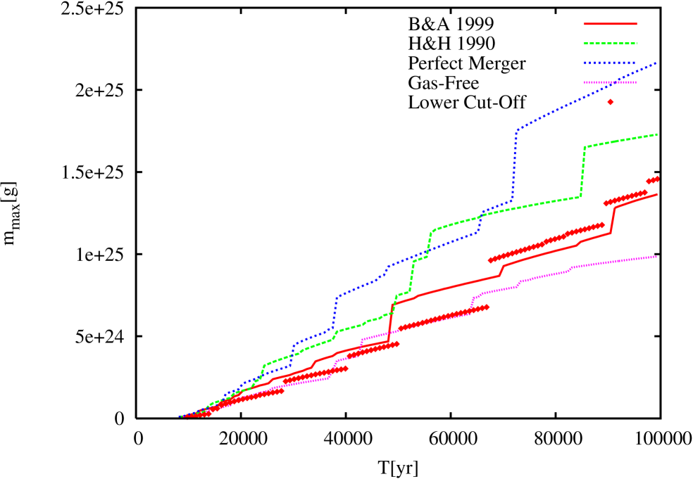
Figure 15: Largest body in the simulation as a function of time for the different collision models S1FB (B&A 1999), S2FH (H&H 1990), S3FN (perfect merger) and S4FBN (gas-free). In addition, we also include simulation S7FB2 with a lower cut-off mass.

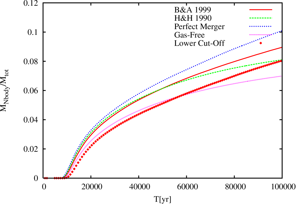
Figure 16: The same as figure 15 for the total mass in the $N-$body component.

A further examination of the mass loss – which we define as the mass in planetesimals which cross the lower grid boundary– reveals the cause of this different behaviour: A pronounced mass loss in simulation S2FH slows down the protoplanetary growth reducing the surface density. In the gas-free case, the accretion rate is mainly reduced because of a larger velocity dispersion, although we can still notice some enhanced mass loss by comparing the lower panels of figures 13 and 14.

We find no accelerated growth due to the inclusion of fragmentation events, contrary to the work of Wetherill (1989). We find that a lower impact strength or the absence of gas damping slows down the growth by an increased mass loss. The total mass in the $N-$body component is still small at the end of the simulations, of about $\approx 10\%$ of the total mass, as shown in table 5 of next section.

3.4 Spatial distribution

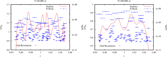
Figure 17: Left y-axis and solid, red curve of the left panel: Radial density structure of the statistical component of model S1FB at $T=3\times 10^{4}$ yr. Right y-axis and blue dots of the left panel: Semimajor axis and masses of the $N-$body particles in the simulation after the same amount of time. The error bars are 10 Hill radii wide and refer to the heating zone of each $N-$body particle. We also display the grid resolution as a reference point. In the right panel we depict the same after $T=10^{5}$ yrs.

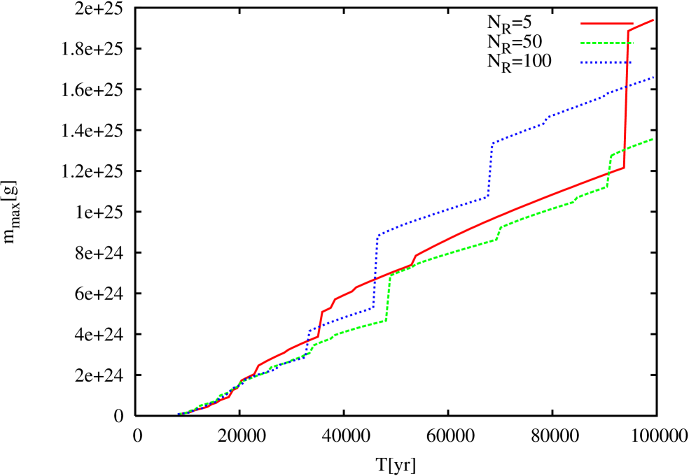
Figure 18: Largest body in the simulation as a function of time for the different resolutions S5FBL $(N_{R}=5)$, S1FB $(N_{R}=50)$ and S6FBH $(N_{R}=100)$.

How well the code can treat spatial inhomogeneities depends on the choice of the spatial resolution. We hence compare a low resolution model, model S5FBL of table 3, which virtually inhibits any spatial structuring, with a model that uses our fiducial resolution, model S1FB, as well as with a model that has a finer resolution, S6FBH. We adjust the fiducial resolution to the width of the heating zone of a planetesimal at the transition mass.

In the left panel of figure 17 we have the spatial structure at $T=30,000$ yr, i. e. shortly after stage D (nominal model S1FB). While the protoplanets are already massive enough after a few $10^{4}$ years (stage C) to open gaps in the planetesimal component, there is only a weak correlation between the radial structures and the location of the most massive protoplanets. A closer examination of the time evolution of the radial structure reveals that most features are “fossils” from the first emerged $N-$body particles, which are slowly washed out by the diffusion of the field planetesimals. In the right panel of the same figure 17 we confirm the further smoothing of the radial features. While major mergers among the protoplanets still lead to distinct features in the surface density even after a few $10^{4}$ years, any further structuring ceases at the end of the simulation.

The absence of any prominent gap formation (fluctuations are smaller than 20 %) is related to the evolution of the overall size distribution. Though the gap opening criterion (see section “Protoplanet growth” of Paper I, and we reproduce here the relevant equation for convenience)

$$\frac{M_{\mathrm{gap}}}{M_{c}} \approx \left\{\begin{array}[]{lll}\frac{\Sigma a^{2}}{M_{c}}\left(\frac{m}{M_{c}}\right)^{{1}/{3}}&\mbox{if}&v\lesssim\Omega r_{\mathrm{Hill}}\\ \frac{\Sigma a^{2}}{M_{c}}\left(\frac{m}{M_{c}}\right)^{1/3}\left(\frac{\Omega r_{\mathrm{Hill}}}{v}\right)^{2}&\mbox{if}&v\gg\Omega r_{\mathrm{Hill}},\end{array}\right.$$ (10)

is formally satisfied by all protoplanets during the runaway phase, the dense overlapping of the associated heating zones (see figure 17) inhibits the evolution of any gap-like feature. As the protoplanets grow, they exert a growing influence on the dynamics of the planetesimal system. While this dominance could in principle enhance gap formation, the system is already dynamically too hot to allow the system to develop radial structures. The eccentricities of the field planetesimals are comparable to the width of the heating zone (compare figure 13, bottom), and hence any planetesimal that is scattered to larger (or smaller) radii immediately encounters a neighbouring protoplanet.

In summary, the protoplanets (or rather their precursors) are too abundant when the system is dynamically cool enough, but when a group of mature protoplanets has evolved, the system is already too hot. Thus, we expect an even less effective radial structuring for larger surface densities. While systems with a lower surface density may lead to the formation of gap-like structures, they evolve slowly that planet formation may never reach the final growth phases.

3.5 Resolution

We can further evaluate the (minor) role of gap formation by comparing the growth process for the three different radial resolutions $N_{R}=5$, $N_{R}=50$ and $N_{R}=100$. Besides some variations due to a different sequence of major impacts (see figure 18), all three simulations are in excellent agreement with respect to the mass loss and the total mass in the $N-$body component.

Accordingly, we find no differences between the various fragmentation models (S1FB, S2FH, S3FN, S4FBN) with respect to possible emerging gaps, except an earlier homogenisation in the gas-free case S4FBN due to the stronger heating of the smaller planetesimals.

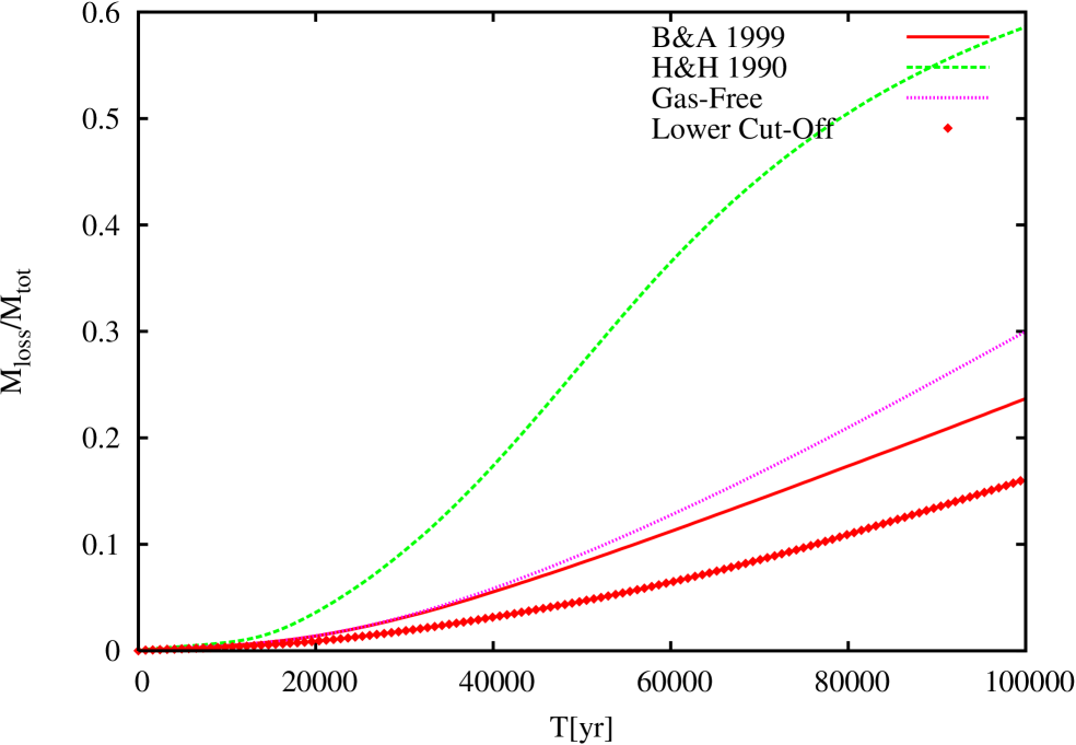
Figure 19: Same as in figure 15 for the total mass loss. For obvious reasons we do not include S3FN, which assumes perfect merger.

We conduct one additional simulation, named S7FB2, see figure 20, in which we reduce the lower mass grid boundary by a factor $10^{5}$. Although the standard choice $m_{\min}=6.9\times 10^{15}$ g is in accordance with the size regime where migration would remove the smaller fragments, the actual mass cut-off is less sharp as we estimated in section “Collisional cascades” of Paper I. A reduced lower cut-off increases the dwell time of collisional fragments in the system, thus increasing the mass fraction which could be accreted by the protoplanets. As a result, mass loss is reduced by 30% compared to our fiducial case S1FB, as we can see in figure 19. AltThough the shape of the fragment tail is modified by a different choice of the grid boundary, the change of the overall evolution of the protoplanets is rather small.

Figure 20: Summary of simulation S7FB2, which uses the B&A 1999 strength and a smaller lower cut-off mass.

3.6 Surface density

Simulation	$\Sigma[$g$/$cm${}^{2}]$	m$[$g$]$	$v_{\mathrm{Hill}}[$m$/$s$]$	$M_{\mathrm{Nbody}}/M_{\mathrm{Statistic}}$	$M_{\mathrm{iso}}$[g]
S8_S2	2	$2.6\times 10^{23}$	10.5	0.04	$7.8\times 10^{25}$
S1FB	10	$1.2\times 10^{25}$	37.6	0.13	$8.6\times 10^{26}$
S9_S100	100	$4.1\times 10^{26}$	122.2	1.34	$2.7\times 10^{28}$

Table 5: Maximum mass and associated quantities at $T=100,000$ years for different surface densities.

We now examine the evolution of different surface densities with a last set of simulations. We take S1FB as our nominal model, with a a surface density of $\Sigma=10$ g$/$cm². We explore two different surface densities: A low–mass disc with $\Sigma=2$ g$/$cm² (simulation S8_S2), and a high–mass disc with $\Sigma=100$ g$/$cm² (simulation S9_S100), which is close to the upper mass limit set by observations. The basic parameters of all three simulations are equal except a proper scaling of the gas density and transition masses chosen individually.

We first resume the inspection of possibly emerging gaps: While the low mass case shows a more pronounced radial structure (with fluctuations as large as 40%), these features are only weakly related to the location of the largest protoplanets. Hence, these structures are signatures of the first emerging $N-$body particles. The high mass case exhibits no strong features at all, except for very weak features during the initial runaway phase. These results strengthen the discussion in Section 3.4, assigning only a minor role to gap formation in the planetesimal component during the protoplanet accretion.

The overall growth process follows a standard pattern. Since the accretion rate in all three simulations is directly proportional to the surface density (see the following equation of section “Protoplanet growth” of Paper I), we rescale the time to the reference simulation S1FB. We obtain a good agreement in the time evolution of the largest mass in the system, as we can see in figure 21, although the turnover to the slower oligarchic growth occurs at different (scaled) times. Likewise, we rescale the time to ease the comparison of the mass loss in the three simulations, which we depict in figure 22.

As soon as a set of dominant protoplanets has evolved, they control the velocity dispersion of the field planetesimals. Therefore the magnitude of the velocity dispersion matches the Hill velocity of the largest body in the system (see Table 5 and figure 13, 24 and 25).

While this similarity in the three simulations is also in good agreement with standard estimations of the growth process (see the section “Initial models” of Paper I), the later stages in the evolution differ markedly: A larger surface density implies larger (and faster growing) protoplanets, so that the velocity dispersion of the field planetesimals is also driven to higher velocities. This therefore leads to an increased mass loss as the initial surface density increases (figure 22). The mass loss of the most massive setup S9_S100 reduces the surface density nearly to the standard case S1FB. Since the mass loss is not due to actual migration of smaller fragments, but to the lower grid boundary (in mass) which mimics the effect of migration, this effect deserves a closer examination:

The influence of fragmentation on the protoplanetary growth is mainly determined by two timescales: The fragmentation time, $\tau_{\mathrm{frag}}$, which refers to collisions between planetesimals, and the growth timescale $\tau_{\mathrm{grow}}$ of the protoplanetary accretion.

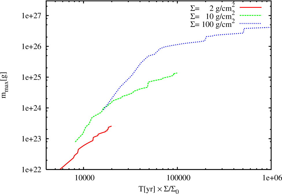
Figure 21: Largest body in the simulation as a function of time for the different surface densities S8_S2 ($\Sigma=2$ g$/$cm²), S1FB ($\Sigma=10$ g$/$cm²) and S9_S100 ($\Sigma=100$ g$/$cm²). The reference density is $\Sigma_{0}=10$ g$/$cm².

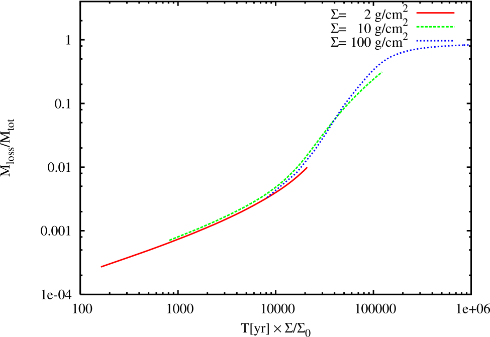
Figure 22: Mass loss in the simulation as a function of time for different surface densities for the same cases of figure 21.

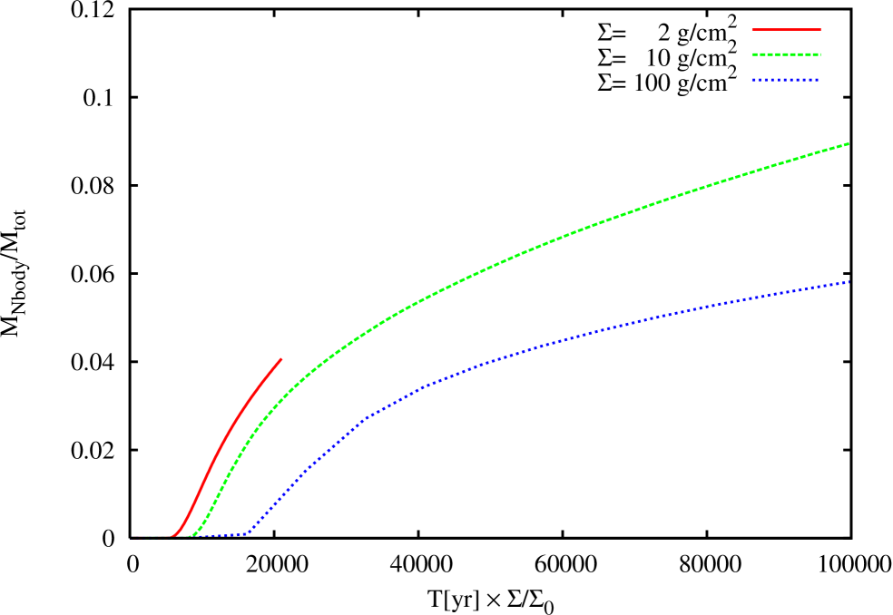
Figure 23: Mass in the $N-$body component of a simulation as a function of time for the different surface densities S8_S2 ($\Sigma=2$ g$/$cm²), S1FB ($\Sigma=10$ g$/$cm²) and S9_S100 ($\Sigma=100$ g$/$cm²).

We employ the expressions derived in section “Perturbation of equilibrium” of Paper I and the approximated differential surface density of equation 7 to estimate the fragmentation time:

$$\tau_{\mathrm{frag}} \approx\frac{\tilde{S}}{G_{0}^{\prime}}\tau_{0}\qquad G_{0}^{\prime}\approx 10$$

$$\approx\frac{\ln(m/m_{0})}{80}\frac{R_{m}S_{m}}{\Sigma_{m}\Omega^{3}R_{\mathrm{Hill}}^{2}}.$$ (11)

In the last equation $m$ is a typical mass of the largest planetesimals, $R_{m}$ is the corresponding radius and $S_{m}$ is the impact strength. $\Sigma_{m}$ is the total surface density of the field planetesimals, with a lower cut-off $m_{0}$ due to migration. $R_{\mathrm{Hill}}$ is the typical Hill radius of a protoplanet, where it is assumed that the protoplanets control the velocity dispersion of the field planetesimals.

4 The mill condition

The growth timescale of the protoplanets follows immediately from rearranging the following equation, as discussed in section “Protoplanet growth” of Paper I:

$$\dot{M}\approx 6\pi\Sigma\Omega\frac{RR_{\mathrm{Hill}}}{\tilde{e}_{m}^{2}}$$ (12)

The timescale hence is

$$\tau_{\mathrm{grow}}\approx\frac{M\tilde{e}_{m}^{2}}{6\pi\Sigma_{m}\Omega RR_{\mathrm{Hill}}}$$ (13)

Since the mass loss due to migration and the replenishment of smaller fragments by mutual collisions quickly establishes a stationary solution, the removal of the field planetesimals operates on the fragmentation timescale. Since the protoplanets grind the surrounding planetesimals without retaining a significant fraction, the accretion of the protoplanet ceases if the condition

$$\tau_{\mathrm{grow}}>\tau_{\mathrm{frag}}$$ (14)

is fulfilled, which we will refer to from now onwards as the “mill condition”. We can easily derive a lower limit for the protoplanet mass assuming $\tilde{e}_{m}=4$ and by translating this condition in terms of mass, the “mill mass”,

$$M >\frac{1}{53}\ln(m/m_{0})\frac{R_{m}S_{m}}{\Omega^{2}}\sqrt[3]{\frac{M_{c}}{a^{3}\rho}},$$ (15)

which we denote as $M_{\mathrm{mill}}$:

$$\frac{M_{\mathrm{mill}}}{m}=\frac{f}{53}\ln(m/m_{0})\left(\frac{2S_{m}}{\rho v_{\infty,m}^{2}}\right)\left(\frac{a^{3}\rho}{M_{c}}\right)^{2/3}$$ (16)

In the last expression $\rho$ is the bulk density of the planetesimals and $v_{\infty,m}$ is the escape velocity of the field planetesimals. $f$ is a factor of order unity to take into account alternative treatments of migration that could alter the size of $M_{\mathrm{mill}}$.

We note that a necessary condition for the mill process to operate is the presence of a gaseous disc. Since a high surface density is needed for the protoplanetary growth to reach the mill mass, the growth itself is likely to be faster than the dispersal of the gaseous disc.

Nevertheless, the concept is also useful in a gas-free system: If the protoplanets in a given planetary system do not exceed the mill mass, it is still possible that the planets after the final giant impact phase exceed $M_{\mathrm{mill}}$. Radiative pressure and Pointing–Robertson drag still provide an effective removal of dust-sized particles in a gas-free system (see the discussion in Burns et al. 1979); hence, while the absence of strong migration of planetesimals prevents any reduction of the planetary accretion rate, the system enters nevertheless a qualitatively different stage: The evolution of the left-over planetesimals (i. e. the disc clearing) is now driven by fragmentation rather than accretion.

The mill mass is that is independent of the surface density of the field planetesimals and hence represents a universal upper limit of the protoplanet mass, given that all other parameters of the planetary system are fixed. The mill mass increases more steeply with radius ($\propto r^{2}$) than the isolation mass for any realistic density profiles (e.g. $M_{\mathrm{iso}}\propto r^{3/4}$ for the minimum mass solar nebula).

Figure 24: Summary of simulation S8_S2, which uses the B&A 1999 strength and a lower surface density $\Sigma=2$ g$/$cm². Table 4 gives the time coding of the labels A–F.

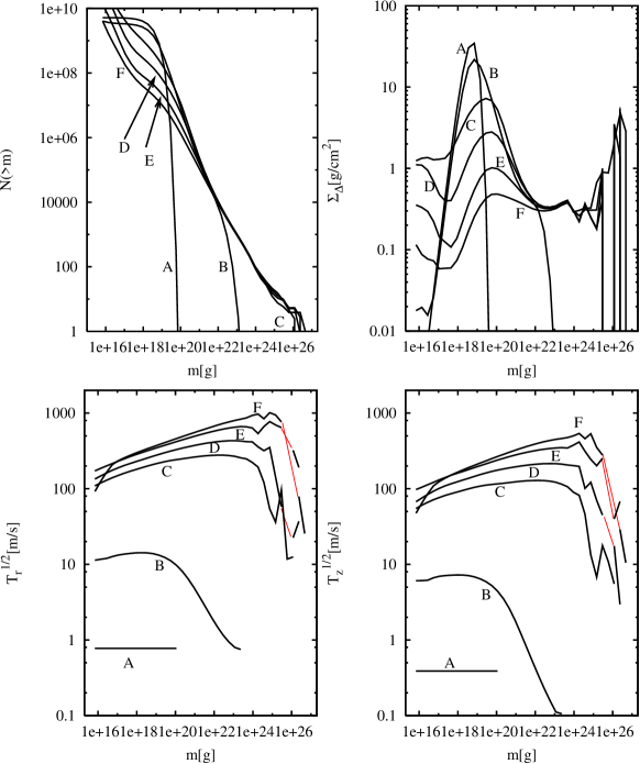
Figure 25: Summary of simulation S9_S100, which uses the B&A 1999 strength and a higher surface density $\Sigma=100$ g$/$cm². Red lines refer to empty mass bins.

This restricts the efficient termination of accretion by fragmentation to the inner parts –e.g. the terrestrial zone in the solar system– of a planetary system. The migration process enters only through the lower cut-off mass $m_{0}$. While the uncertainty of $m_{0}$ in principle is not a big issue, as it appears in the logarithm, the truth is that the migration timescale depends on the planetesimal radius which can vary significantly. An uncertainty of the cut-off radius by a factor of ten indicates an uncertainty of $M_{\mathrm{mill}}$ of the same order, which again leads us to the question about the necessity of a careful treatment of migration in a global frame.

All simulations use a lower cut-off size of $800$ metres, which is roughly equivalent to the cut-off introduced by migration. Since $m_{0}$ is defined by the identity of the migration timescale and the fragmentation timescale (see section “Collisional cascades” of Paper I), this mass is also independent of the surface density, given that the ratio of solid to gaseous material is constant. While the more refined simulation S6FBH shows a mass loss only reduced by 30%, we expect that the uncertainty due to the reduced treatment of migration to be at least of the same order.

In view of these considerations, we retake now the analysis of the simulations: Simulation S9_S100 is strongly affected by the mill process, whereas simulation S1FB still retains a significant fraction of the initial mass. The quiescent conditions in simulation S8_S2 exclude a prominent role of fragmentation at any evolutionary stage. Thus we estimate $M_{\mathrm{mill}}\approx 0.1M_{\oplus}$ for a solar system analogue at 1 AU (see figure 21), which yields the approximate expressions:

$$M_{\mathrm{mill}} =f\times 0.1\,M_{\oplus}\times\left(\frac{r}{1{AU}}\right)^{2}\left(\frac{M_{c}}{1\,M_{\odot}}\right)^{-2/3}$$

$$\left(\frac{\rho}{2.7\,{g/cm}^{3}}\right)^{2/3}$$ (17)

Since the protoplanets maintain a separation of approximately $10\,R_{\mathrm{Hill}}$, the mill mass corresponds to an upper limit $\Sigma_{\mathrm{mill}}$ of the surface density which is available for the formation of protoplanets:

$$\Sigma_{\mathrm{mill}} =\frac{M_{\mathrm{mill}}}{20\pi aR_{\mathrm{Hill}}}$$

$$=f^{2/3}\times 9.15\,\frac{\mathrm{g}}{\mathrm{cm}^{2}}\times\left(\frac{r}{1{AU}}\right)^{-2/3}\left(\frac{M_{c}}{1\,M_{\odot}}\right)^{-1/9}$$

$$\left(\frac{\rho}{2.7\,{g/cm}^{3}}\right)^{4/9}$$ (18)

The scaling relation 17 implies $M_{\mathrm{mill}}\approx 2.5\,M_{\oplus}$ at 5 AU, which is in agreement with an upper core mass of $4M_{\oplus}$ found in the simulations of Inaba et al. (2003). Although it seems impossible to form a core that is large enough ($15\,M_{\oplus}$) to initiate gas accretion, this tight upper limit is due to disregarding the gaseous envelope –i. e. the protoplanetary atmosphere before the onset of strong gas accretion– of the growing core. Since the gaseous envelope enhances the accretion cross section by an order of magnitude (and hence $f\approx 10$ in equation 17), the mill mass increases by the same factor. Thus the formation of a $15\,M_{\oplus}$ proto-jovian core at 5 AU is not ruled out by fragmentation, again in agreement with Inaba et al. (2003).

Both low–mass simulations S1FB and S8_S2 still contain a major fraction of the total mass in the statistical component, which prevents the onset of orbital crossing on a timescale of a few $10^{5}$ years. However, the fast protoplanetary growth in the high–mass simulation S9_S100, accompanied by an intense mass loss, leads to an onset of strong protoplanet–protoplanet interactions already at the end of the simulation. The chaotic evolution of the velocity dispersion at the high mass end, as we can see in figure 25 bottom, indicates an intense interaction of the $N-$body particles.

5 Discussion

In this article, which can be envisaged as a continuation of the work we presented in Paper I, we first carefully assess the code and then apply it to investigate the formation of protoplanets. Our main results are summarised as follows

1. The influence of the fragmentation model on the protoplanetary growth is weak during the fast initial runaway growth. In particular, any realistic choice of the impact strength does not inhibit the growth of the planetesimals. However, the choice of the fragmentation model controls the oligarchic growth through the overall mass loss due to the migration of smaller fragments. Our simulations show that the Housen & Holsapple (1990) strength leads to a significant deceleration of the mass accretion in the later phases. Thus the recent impact strength from Benz & Asphaug (1999) is more favourable in terms of an efficient protoplanet formation.

2. We derive the notion of a critical mill mass to provide a convenient handle on the fragmentation processes. If the mass of a (proto)planet exceeds this critical limit, then an interplay of destructive collisions and the removal of fragments by migration terminates the accretion of planetesimals. In particular, this critical mass implies an upper limit of the mass (in solids), which can be transformed into planets, unless migration ceases very early due to the fast dissipation of the gaseous disc.

3. Contrary to the work of Rafikov (2001), we find no termination of the protoplanetary accretion due to gap formation. None of our simulations shows any significant radial structure, except for a limited time during the runaway accretion. While low surface densities favour gap formation, all observed radial features are so weak that the notion “gap” does not correspond to these structures. Hence, resonant interactions between protoplanets and the field planetesimals are not a dominant process during the growth phases considered, which also supports the validity of the Fokker–Planck approach. Likewise, the dynamically hot field planetesimals also suppress non-axisymmetric features beyond the Hill radius of the protoplanets. We must mention that the difference we find with Rafikov (2001) is true for a hot disc. Nevertheless, his solution is correct in some cases, especially when the disc can remain cold (see Ida et al. 2000; Kirsh et al. 2009) as in, for instance, the gaps of Saturn’s rings ( e.g. the work of Goldreich & Tremaine 1978b, a; Lissauer et al. 1981).

The eccentricity and inclination of the protoplanets remain small during the oligarchic growth phase. However, we note that this does not imply small eccentricities of the final planets, since the onset of orbital crossing terminates the dynamically quiet oligarchic growth phase.

Since our work introduced a new computer code to study the growth of protoplanets, we primarily focussed on the careful assessment of its validity and a small parameter study to strengthen this approach. Considering that the current abilities of the hybrid code exclude global simulation which could address migration in a proper way, we restricted our studies to a small ring of planetesimals. However, our experience drawn from this work allows an outline of possible improvements. The wallclock time of a rather small simulation is dominated by the integration of the statistical component. As the radial extension of the simulation volume is increased, the computing time due to the statistical component increases linearly, whereas the computing time due to the $N-$body component increases proportional to the square of the radial width. If the resolution of the radial grid is reduced, the weight of the $N-$body part will further increase. A moderately extended model, which covers the inner planetary system up to 10 AU, requires the long-term integration of $10^{3}$ to $10^{4}$ particles.

While these are only few particles compared to big star cluster simulations (e.g. Makino 2004; Berczik et al. 2005), the long integration times of at least $10^{6}$ orbits prevent the efficient parallelisation. Astrophysicists had an early start in the field of through the GRAPE hardware in a standard PC cluster (see the extensive description in Fukushige et al. 2005). A more promising solution are the modern graphics processing units (GPUs), which have made significant progress in the last years. They were originally used to perform calculations related to 3D computer graphics. Nevertheless, due to their highly parallel structure and computational speed, they can be very efficiently used for complex algorithms. Computational astrophysics has been a pioneer to use GPUs for high performance general purpose computing (see for example the early AstroGPU workshop in Princeton 2007, through the information base). The direct $N-$body code has been ported to GPUs by Sverre Aarseth who, as is his admirable custom, has made the code publicly available. We plan on porting our hybrid method to GPU technology soon.

The extension of the simulations towards longer integration times does not only require an optimisation of the hybrid code, but also a more careful modelling of the growing planets to account for the interaction with the gaseous disc. While these improvements are necessary to allow the consistent treatment of migration, they also open the study of the early debris disc phase. Debris discs could provide constraints on the planet formation process, since the low opacity of kilometre-sized planetesimals prevents the direct observation of the protoplanetary growth in extrasolar systems. Though all these improvements are not implemented yet, they encourage us to pursue the further development of the hybrid approach.

References

- Aarseth (1999) Aarseth S., 1999, PASP, 111, 1333
- Aarseth (2003) —, 2003, Cambridge University Press
- Armitage (2010) Armitage P. J., 2010, ArXiv e-prints
- Benz & Asphaug (1999) Benz W., Asphaug E., 1999, Icarus, 142, 5
- Berczik et al. (2005) Berczik P., Merritt D., Spurzem R., 2005, Astrophysical Journal, 633, 680
- Burns et al. (1979) Burns J., Lamy P., Soter S., 1979, Icarus, 40, 1
- Fukushige et al. (2005) Fukushige T., Makino J., Kawai A., 2005, PASJ, 57, 1009
- Goldreich et al. (2004) Goldreich P., Lithwick Y., Sari R., 2004, Annu. Rev. Astron. Astrophys., 42, 549
- Goldreich & Tremaine (1978a) Goldreich P., Tremaine S. D., 1978a, Icarus, 34, 240
- Goldreich & Tremaine (1978b) —, 1978b, Icarus, 34, 227
- Housen & Holsapple (1990) Housen K. R., Holsapple K. A., 1990, Icarus, 84, 226
- Ida et al. (2000) Ida S., Bryden G., Lin D. N. C., Tanaka H., 2000, ApJ, 534, 428
- Inaba et al. (2001) Inaba S., Tanaka H., Nakazawa K., Wetherill G., Kokubo E., 2001, Icarus, 149, 235
- Inaba et al. (2003) Inaba S., Wetherill G., Ikoma M., 2003, Icarus, 166, 46
- Khalisi et al. (2007) Khalisi E., Amaro-Seoane P., Spurzem R., 2007, MNRAS
- Kirsh et al. (2009) Kirsh D. R., Duncan M., Brasser R., Levison H. F., 2009, Icarus, 199, 197
- Kokubo (1995) Kokubo E., 1995, Icarus, 114, 247
- Kokubo (1996) —, 1996, Icarus, 123, 180
- Lissauer (1993) Lissauer J., 1993, Annu. Rev. Astron. Astrophys., 31, 129
- Lissauer et al. (1981) Lissauer J. J., Shu F. H., Cuzzi J. N., 1981, Nat, 292, 707
- Makino (2004) Makino J., 2004, Astrophysical Journal, 602, 93
- Ohtsuki et al. (2002) Ohtsuki K., Stewart G., Ida S., 2002, Icarus, 155, 436
- Rafikov (2001) Rafikov R., 2001, Astronomical Journal, 122, 2713
- Rafikov (2003) —, 2003, Astronomical Journal, 126, 2529
- Spurzem (1999) Spurzem R., 1999, The Journal of Computational and Applied Mathematics, Special Volume Computational Astrophysics, 109, 407
- Wetherill (1989) Wetherill G., 1989, Icarus, 77, 330
- Wetherill (1993) —, 1993, Icarus, 106, 190