Abstract

This note investigates a number of scenarios in which unadjusted testing following a blinded sample size re-estimation leads to type I error violations. For superiority testing, this occurs in certain small-sample borderline cases. We discuss a number of alternative approaches that keep the type I error rate. The paper also gives a reason why the type I error inflation in the superiority context might have been missed in previous publications and investigates why it is more marked in case of non-inferiority testing.

1 Introduction

Sample Size re-estimation (SSR) in clinical trials has a long history that dates back to Stein (1945). A sample size review at an interim analysis aims at correcting assumptions which were made at the planning stage of the trial, but turn out to be unrealistic. When the sample units are considered to be normally distributed, this typically concerns the initial assumption about the variation of responses. Wittes and Brittain (1990) and Gould and Shih (1992, 1998) among others discussed methods of blinded SSR. In contrast to unblinded SSR, blinded SSR assumes that the actually realized effect size estimate is not disclosed to the decision makers who do the SSR. Wittes et al. (1999) and Zucker et al. (1999) investigated the performance of various blinded and unblinded SSR methods by simulation. They observed some slight type I error violations in cases with small sample size and gave explanations for this phenomenon for some of the unblinded approaches available at that time.

Slightly later, Kieser and Friede([1], [2]) suggested a method of blinded sample size review which is particularly easy to implement. In a trial with normally distributed sample units with the aim of testing for a significant treatment effect (”superiority testing”) at the final analysis, it estimates the variance under the null hypothesis of no treatment effect and then proceeds to an unmodified $t$-test in the final analysis, i.e. a test that ignores the fact that the final sample size was not fixed from the onset of the trial. Kieser and Friede investigated the type I error control of their suggestion by simulation. They conclude that no additional measures to control the significance level are required in these designs if the study is evaluated with the common t-test and the sample size is recalculated with any of these simple blind variance estimators.

Although Kieser and Friede explicitly stated that they provide no formal proof of type I error control, it seems to us that many statisticians in the pharmaceutical industry are under the impression that such a proof is available. This, however, is not the case. In this paper, we show that in certain situations, the method suggested by Kieser and Friede does not control the type I error.

It should be emphasized that asymptotic type I error control with blinded SSR is guaranteed. If the sample size of only one of the two stages tends to infinity, the other stage is obviously irrelevant for the asymptotic value of the final test statistic and thus the method asymptotically keeps $\alpha$. If the sample size in both stages goes to infinity, then the stage-1-estimate of the variance converges to a constant value. Hence, whatever sample size re-estimation rule is used, it implicitly fixes the total sample size in advance (though its precise value is not yet known before the interim). In any case, asymptotically $\alpha$ is again kept. Govindarajulu (2003) has formalized this thought and extended to non-normally distributed data. As a consequence, the type I error violations discussed in this note are very small and occur in cases with small samples. We still believe, however, that the statistical community should be made aware of these limitations of blinded sample-size review methodology.

While sections 2-4 focus on the common case of testing for treatment differences in clinical trials, section 5 briefly discusses the case of testing for non-inferiority of one of the two treatments. In had been noted in another paper by Friede and Kieser [13] that type I error inflations from SSR can be more marked in this situation. We give an explanation of this phenomenon.

2 A scenario leading to type I error violation

In this section we show that in certain cases, a blinded sample size review as suggested by [1] leads to a type I error which is larger than the nominal level $\alpha$.

In general, blinded sample review is characterized by the fact that the final sample size of the study may be changed at interim analyses, but that this change depends on the data only via the total variance which is the variance estimate under the null hypothesis of interest. If $x_{i},i=1,\ldots,n_{1}$ are stochastically independent normally distributed observations, this total variance is proportional to $\sum_{i=1}^{n_{1}}x_{i}^{2}$ in the one-sample and to $\sum_{i=1}^{n_{1}}x_{i}^{2}-n_{1}\bar{x}^{2}$ in the two-sample case.

We consider the one-sample $t$ test of $H_{0}:\mu=0$ at level $\alpha$ applied to $x_{i}\sim N(\mu,\sigma^{2})$. The reason for this is simplicity of notation and the fact that the geometric considerations given below cannot be imagined for the two-sample case which would have to deal with a dimension larger than three even in the simplest setup. However, the restriction to the one-sample case entails no loss of generality, as it is conceptually the same as the two sample case. We will briefly comment on this further below. In addition, a blinded sample size review may also be of practical relevance in the one-sample situation, for example in cross-over trials.

Assume a blinded sample size review after $n_{1}=2$ observations. If the total variance is small, we stop sampling and test with the $n_{1}=n=2$ observations we have obtained. If it is large, we take another sample element $x_{3}$, and do the test with $n=3$ observations. This rule implies that $n=2$ for $x_{1}^{2}+x_{2}^{2}\leq r^{2}$ and $n=3$ otherwise for some fixed scalar $r$. Geometrically, the rejection region of the (one-sided) $t$ test for $n=3$ is a spherical cone with the equiangular line $x_{1}=x_{2}=x_{3}$ as its central axis in the three-dimensional space. By definition, the probability mass of this cone is $\alpha$ under $H_{0}$. For the case of $n=2$, the rejection region is a segment of the circle $x_{1}^{2}+x_{2}^{2}\leq r^{2}$ around the equiangular line $x_{1}=x_{2}$. Hence, in three dimensions, the rejection region is a segment of the spherical cylinder $x_{1}^{2}+x_{2}^{2}\leq r^{2},x_{3}$ arbitrary. The probability mass covered by this segment again is $\alpha$ inside the cylinder. The rejection region of the entire procedure is the segment of the cylinder plus the spherical cone minus the intersection of the cone with the cylinder. We now approximate the probability mass of these components.

For $r^{2}$ small, we approximately have $P(x_{1}^{2}+x_{2}^{2}\leq r^{2})=\frac{r^{2}}{2\sigma^{2}}$. Hence, under $H_{0}$, the probability mass of this part of the rejection region is approximately $\frac{r^{2}}{2\sigma^{2}}\cdot\alpha$. The volume of the intersection of the cone with the cylinder can be approximated as follows: The central axis $x_{1}=x_{2}=x_{3}$ of the cone intersects with the cylinder in one of the points $\pm\left(\frac{r}{\sqrt{2}},\frac{r}{\sqrt{2}},\frac{r}{\sqrt{2}}\right)$. The distance of this point to the origin is thus $h=\sqrt{\frac{3}{2}}r$. The approximate volume of the intersection is $\frac{4\pi h^{3}}{3}=\sqrt{6}\pi r^{3}$. To conservatively approximate the probability mass of this intersection, we assume that every point in it has the same probability mass as the origin (in reality, it of course has a lower probability mass). Then the probability mass of the intersection is approximated by $\sqrt{6}\pi r^{3}\cdot\alpha\cdot(\sqrt{2\pi}\sigma)^{-3}$, where $(\sqrt{2\pi}\sigma)^{-3}$ is the value of the standard normal density $N_{3}\left(\mathbf{0},\sigma^{2}\mathbf{I}_{3}\right)$ in the point $\mathbf{0}$. Combining these results, a conservative approximation of the probability mass of the rejection region for the entire procedure is

$$\alpha\left(1+\frac{r^{2}}{2\sigma^{2}}-\frac{\sqrt{6}\pi r^{3}}{(\sqrt{2\pi}\sigma)^{3}}\right)=\alpha\left(1+\frac{r^{2}}{2\sigma^{2}}-\frac{\sqrt{3}r^{3}}{2\sqrt{\pi}\sigma^{3}}\right).$$ (1)

Obviously, this is larger than $\alpha$ for small $r$.

For the more general case of a stage-1-sample size of $n_{1}$, possibly followed by a stage 2 with $n_{2}$ further observations, the rejection region of the ”sample size reviewed” $t$ test has an approximate null probability following the same basic principle as (1):$\alpha\cdot\left(1+const_{1}\cdot\left(\frac{r}{\sqrt{n_{1}}\sigma}\right)^{n_{1}}-const_{2}\cdot\left(\frac{r}{\sqrt{n_{1}}\sigma}\right)^{n_{1}+n_{2}}\right)$ if $r,n_{1}$ and $n_{2}$ are small. Consequently, there must be situations with small $\frac{r}{\sqrt{n_{1}}\sigma}$ where the blinded review procedure cannot keep the type I error level $\alpha$ exactly. Due to symmetry of the rejection region, this statement holds for both the one- and the two-sided test of $H_{0}$.

Note that in this example, the test keeps $\alpha$ exactly if $\sum_{i=1}^{n_{1}}x_{i}^{2}\leq r^{2}$. This is due to the sphericity of the conditional null distribution of $(x_{1},\cdots,x_{n_{1}})$ given $\sum_{i=1}^{n_{1}}x_{i}^{2}\leq r^{2}$ (see [3], theorem 2.5.8). Type I error violation stems from the fact that the test does not keep $\alpha$ conditional on $\sum_{i=1}^{n_{1}}x_{i}^{2}>r^{2}$, i.e. if a second stage of sampling more observations is done.

To investigate the magnitude of the ensuing type I error violation, we simulated 10’000’000 cases with $n_{1}=2$ initial observations and $n_{2}=2$ additional observations that are only taken if $x_{1}^{2}+x_{2}^{2}\geq 0.5$. The true type I error of the two-sided combined $t$ test turned out to be $0.0542$ for a nominal $\alpha=0.05$. As expected, this is caused by the situations where stage-2-data is obtained. Since $x_{1}^{2}+x_{2}^{2}\sim\chi^{2}(2)$, we have $P(x_{1}^{2}+x_{2}^{2}\geq 0.5)=0.779$. This was also the value observed in the simulations. The rejection rate for these cases alone was $0.0553$. If $x_{1}^{2}+x_{2}^{2}<0.5$, we know that conditionally the rejection rate is exactly $\alpha$. Accordingly, this conditional rejection rate in the simulations was $0.0500$.

If $n_{1}$ and $n_{2}$ are increased, the true type I error rate converges rather quickly to $\alpha$. For example, in case of $n_{1}=n_{2}=5$ and $r^{2}=2.5$, the simulated error rate is $0.0508$ with $77.6\%$ of cases leading to stage 2 and a conditional error rate of $0.0510$ in case stage 2 applies.

We also performed some simulations where $n_{2}$ is determined with the algorithm suggested by [1]. For this purpose, we generated $10^{\prime}000^{\prime}000$ simulation runs of a blinded sample size review after $n_{1}=2$ observations following the rule given in section 3 of [1] with a very large assumed effect of $\delta=2.2$. This produces an average of $3.09$ additional observations $n_{2}$. The simulated type I error was $0.05077$.

To see that the two-sample case is also covered by these investigations, note that the ordinary $t$-test statistic can be viewed as $X/\sqrt{Y/s}$ where $X\sim N(\delta,1)$ is stochastically independent of $Y\sim\chi^{2}\left(s\right)$. Regarding any investigation of the properties of this quantity, it obviously does not matter if the random variables $X$ and $Y$ arise as mean and variance estimate from a one-sample situation or as difference in means and common within-group variance estimate in the two-sample case. The same is true here: According to [1], p. 3575, the ”resampled” $t$-test statistic consists of the four components $D_{1}$, $V_{1}$, $D_{2}\left|\left(V_{1},D_{1}\right)\right.$ and $V_{2}^{*}\left|\left(V_{1},D_{1}\right)\right.$ (loosely speaking, these correspond to the differences in means and variance estimates of the two stages). Comparing the distributions of $D_{1}$ and $V_{1}$ and the conditional distributions of $D_{2}$ and $V_{2}^{*}$ given $D_{1}$ and $V_{1}$ (and hence $n_{2}$), one immediately sees that these are the same for the one- and the balanced two-sample case when we replace $n_{i}$ by $n_{i}/2$ and the means of the two stages by the corresponding two differences in means between the two treatment groups. For the conditional distribution of $V_{2}^{*}\left|\left(V_{1},D_{1}\right)\right.$ see section 4.

3 Approaches that control the type I error

3.1 Permutation and rotation tests

If the considerations from the previous section are of concern, then a simple alternative is to do the test as a permutation test. In the one-sample case, one would generate all permutations (or a large number of random permutations) of the signs onto the absolute values of observations. For each permutation, the $t$ test would be calculated and the $(1-\alpha)$-quantile of the resulting empirical distribution of $t$-test values gives the critical value of an exact level $\alpha$-test of $H_{0}$. Alternatively, a $p$-value can be obtained by counting the percentage of values from the permutation distribution which are larger or equal to the actually observed value of the test statistic. After determining the additional sample size $n_{2}$ from the first $n_{1}$ observations, we apply the permutation method to all $n_{1}+n_{2}$ observations. The special case of $n_{2}=0$ is possible and then the parametric (non-permutation) $t$-test can also be used. This strategy keeps the $\alpha$-level exactly, because the total variance $\frac{1}{n_{1}}\sum_{i=1}^{n_{1}}x_{i}^{2}$ is invariant to the permutations.

In the two-sample case, the approach would permute the treatment allocations of the observations. In order to preserve the observed total variance, the permutations have to be done separately for the $n_{1}$ observations of stage 1 and the $n_{2}$ observations of stage 2, respectively.

If sample sizes are small, permutation tests suffer from the discreteness of the resampling distribution and the associated loss of power. In this case, rotation tests [4, 5] offer an attractive alternative. These replace the random permutations of the sample units by random rotations. This renders the support of the corresponding empirical distribution continuous and thus avoids the discreteness problem of the permutation strategy. In order to facilitate this, rotation tests require the assumption of a spherical null distribution. This is the case in this context. Stage-1- and stage-2-data have to be rotated separately even in the one-sample case in order to keep the fixed observed stage-1-value of the total variance.

Permutation and rotation strategies emulate the true distribution of the $t$ test including sample size review. Hence, they will ”automatically” correct any type I error inflation as outlined in the previous section, but will otherwise have almost identical properties (e.g. with respect to power) as their ”parametric” counterpart. We did some simulations of the permutation and rotation strategies under null and non-null scenarios. These, however, just backed up the statements made here and are thus not reported.

3.2 Combinations of test statistics from the two stages

Methods that use a combination of test statistics from the two stages are another alternative if one is looking for an exact test. For example, we might use Fisher’s $p$-value combination $-2\log(p_{1}\cdot p_{2})$ [6] where $p_{j}=P(T_{j}>t_{j})$ with $T_{j}$ being the test statistic from stage-$j$-data only and $t_{j}$ its observation from the concrete data at hand. As $-2\log(p_{1}\cdot p_{2})\sim\chi^{2}(4)$ for independent test statistics $T_{1}$ and $T_{2}$ under $H_{0}$, the combination $p$-value test rejects $H_{0}$ if $-2\log(p_{1}\cdot p_{2})$ is larger than the $(1-\alpha)$-quantile from this distribution. In this application, we use the true null distributions of the test statistics $T_{j}$ to determine the $p$-values. For example, in case of the one-sample-$t$-test these are the $t$-distributions $T_{1}\sim t(n_{1}-1)$ and $T_{2}\sim t(n_{2}-1)$.

The stage-2-sample size $n_{2}$ is uniquely determined by $\sum_{i=1}^{n_{1}}x_{i}^{2}$. Since $T_{1}$ is a test statistic for which Theorem 2.5.8. of [3] holds under $H_{0}$, the null distribution of $T_{1}$ is valid also conditionally on $\sum_{i=1}^{n_{1}}x_{i}^{2}$. As a consequence, $T_{1}\sim t(n_{1}-1)$ and $T_{2}\sim t(n_{2}-1)$ are stochastically independent under $H_{0}$ for given $\sum_{i=1}^{n_{1}}x_{i}^{2}$. Any combination of them can be used as the test statistic for $H_{0}$. Of course, one still has to find critical values of the null distribution for the selected combination.

The statement about the conditional null distributions of the test statistics given the total variance $\sum_{i=1}^{n_{1}}x_{i}^{2}$ allows us to go beyond Fisher’s $p$-value combination and similar methods that are combining $p$-values using fixed weights or calculate conditional error functions with an ”intended” stage-2-sample size. The weights used to combine the two stages may also depend on the observed stage-1-data. For example, if the variance were known (and hence a $z$-test for $H_{0}$ could be done), then the optimal (standardized) weights for combining the $z$-statistics from the two stages would be $\sqrt{\frac{n_{1}}{n_{1}+n_{2}}}$ and $\sqrt{\frac{n_{2}}{n_{1}+n_{2}}}$ in the one-sample case. Hence, $t_{comb}=\sqrt{\frac{n_{1}}{n_{1}+n_{2}}}t_{1}+\sqrt{\frac{n_{2}}{n_{1}+n_{2}}}t_{2}$ seems a promising candidate for a combination test statistic. The fact that $\left\{T_{j}\right\},j=1,2$ retain their $t(n_{j}-1)$-null distributions if we condition on $s_{1}^{2}=\sum_{i=1}^{n_{1}}x_{i}^{2}$ means that critical values for this test can be obtained from the distribution of the weighted sum of two stochastically independent $t$-distributed random variables with $(n_{1}-1)$ and $(n_{2}-1)$ degrees of freedom, respectively. It is obvious that this is very easy with numerical integration or a simulation. Comparing $t_{comb}$ with these critical values (that depend only on $n_{1}$ and $n_{2}$) to decide about the rejection of $H_{0}$ gives an exact level-$\alpha$ test.

To investigate the performance of the introduced suggestions, we did several simulations. The critical values for the one-sided one-sample test using $t_{comb}$ were obtained by simulating 1’000’000 values of two independent $t$-distributions with $n_{1}$ fixed and $n_{2}$ as determined by the SSR method in [1]. We used the ”total variance” for SSR, not the ”adjusted variance” which subtracts a constant based on the putative effect size. Nevertheless, the re-estimated sample size of course depends on the ”assumed effect” which may be different from the true, unknown effect size. In the simulations,we investigated various combinations of the true effect size $\mu$ and an assumed effect size $\delta$.

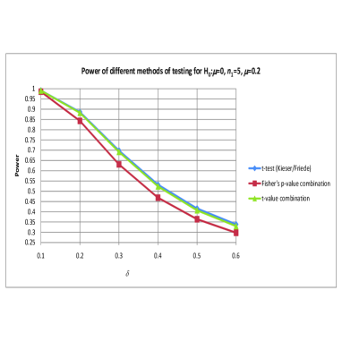
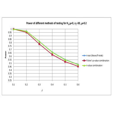
Figure 1: Power of various test after sample size re-estimation

Null simulations verified the claimed type-I-error control for the various adjustment methods described in this section and are thus not reported. Figure 1 shows the results of 1’000’000 simulation runs for sample sizes of $n_{1}=5$ and $n_{1}=30$, a true effect size of $\mu=0.2$ (the standardized true effect size, such that the non-centrality parameter of a standard-$t$-test with $n$ observations would be $\sqrt{n}\mu$) and varying values of $\delta$ on the $x$-axis. The unmodified $t$-test as suggested by [1] is always best. In comparison, the weighted $t$-test combination $t_{comb}$ suffers from a small power loss which seems non-negligible only for very small stage-1-sample sizes below $n_{1}=10$ (where the type I error control of the ”reviewed” $t$-test might be a concern). For all simulated scenarios with $n_{1}=30$, the difference in power was always below $1\%$. In contrast, Fisher’s $p$-value combination typically loses 3 to 4 % of power when $t$-test power is less than 95 % and up to 7% for some scenarios ($\mu=0.1,\delta=0.15$ with power $t$-test 76.4%, power $t$-combination 76.3%, power $p$-value combination 69.6%).

4 The distribution of Kieser and Friede’s $t$-test statistic

To investigate the type I error of the $t$-test after a blinded sample size review, Kieser and Friede [1] write the $t$-test statistic as a function of four components $D_{1}$, $V_{1}$, $D_{2}$ and $V_{2}^{*}$ (see page 3575 of [1]) for which they derive respective distributions. However, the distribution of $V_{2}^{*}$ given $(D_{1},V_{1})$ mentioned there is an approximation, not the exact distribution. Hence, the ”actual” type I error rates in [1] are also approximate, possibly masking a minor type I error level inflation.

The following uses the notation from [1]. It shows that the conditional distribution of $V_{2}^{*}|(V_{1},D_{1})$ is not $\chi^{2}(2n_{2})$.

Without loss of generality it can be assumed that $\sigma^{2}=1$. We have

$$V_{2}^{*}=V_{2}+\frac{n_{1}n_{2}}{n_{1}+n_{2}}\left(\left(\overline{X}_{11}-\overline{X}_{21}\right)^{2}+\left(\overline{X}_{12}-\overline{X}_{22}\right)^{2}\right)$$

$V_{2}|(V_{1},D_{1})\sim\chi^{2}(2n_{2}-2)$ is obvious. It is also obvious that if we condition on $V_{1}$ only, and suppose that this determines sample size $n_{2}$ uniquely, we have

$$D^{*}_{i}:=\sqrt{\frac{n_{1}n_{2}}{n_{1}+n_{2}}}\left(\overline{X}_{1i}-\overline{X}_{2i}\right)\sim N(0,1),$$

such that $D^{*}_{1}$ and $D^{*}_{2}$ are stochastically independent. Thus, in this case $D^{*2}_{1}+D^{*2}_{2}\sim\chi^{2}(2)$, so if $n_{2}$ is a function of $V_{1}$, but not $D_{1}$, the claim $V_{2}^{*}|V_{1}\sim\chi^{2}(2n_{2})$ holds. This was noted by [7].

If we condition on both $V_{1}$ and $D_{1}$, $V_{2}$ and $\left(D^{*}_{1},D^{*}_{2}\right)$ are still independent, but $D^{*}_{1}$ and $D^{*}_{2}$ are no longer.

By applying a theorem on conditional normal distributions (see e.g. [8], page 35) and some well-known results on matrix decompositions, it can be shown that the true conditional distribution of $V_{2}^{*}$ is a mixture distribution:

$$V_{2}^{*}|(V_{1},D_{1})=_{d}\chi^{2}_{2n_{2}-1}+z_{2}^{2},$$

where ”$=_{d}"$ denotes ”equal in distribution” and $z_{2}^{2}$ has the ”rescaled” non-central $\chi^{2}$-distribution

$$z_{2}^{2}\sim\frac{n_{1}}{n_{1}+n_{2}}\cdot\chi^{2}\left(1;\frac{n_{2}}{n_{1}}\left(D_{1}-\sqrt{\frac{n_{1}}{2}}\Delta\right)^{2}\right).$$

The assumption $V_{2}^{*}|(V_{1},D_{1})\sim\chi^{2}(2n_{2})$ will often very closely approximate this real distribution.

5 Sample size reviews when testing for non-inferiority

The preceding sections have dealt with the superiority test $H_{0}:\mu=0$. While type I error violations in this context are extremely small, it was noted by [13] that more serious violations arise in the case of non-inferiority and equivalence testing and that these are persistent with larger sample sizes. This section gives an intuitive explanation for this.

Assume that in the two-sample case, it is intended to test the non-inferiority hypothesis $H_{0}:\mu_{1}-\mu_{2}\leq\delta$ on data $x_{ijk}\sim N\left(\mu_{j},\sigma^{2}\right)$ where $i=1,2$ indexes stage, $j=1,2$ treatment group, $k=1,\ldots,n_{i}$ sample unit and $\delta$ is a fixed non-inferiority margin. Sample size reassessment after stage 1 determines the stage-2-sample size via

$$n_{2}=4\cdot\frac{\left(u_{1-\alpha}+u_{1-\beta}\right)^{2}}{\left(\theta-\delta\right)^{2}}\cdot\tilde{\sigma}^{2}$$ (2)

(where $u_{\alpha}$ is the $\alpha$-quantile of $N(0,1)$, $\beta$ is the desired power of the ordinary two-sample $t$-test and $\theta$ is the assumed true effect difference between the treatments) as a function of the ”total variance”

$$\tilde{\sigma}^{2}=\frac{1}{2n_{1}-1}\sum_{j=1}^{2}\sum_{k=1}^{n_{1}}\left(x_{1jk}-\bar{x}_{1}\right)^{2}$$

with $\bar{x}_{1}=\frac{\sum_{j=1}^{2}\sum_{k=1}^{n_{1}}x_{1jk}}{2n_{1}}$. This, however, does not correspond to a ”blinded” sample size review of the corresponding superiority test. To see this, notice that the described test can also be represented as a test of $H_{0}:\mu_{1}^{*}-\mu_{2}\leq 0$ on the ”shifted” data

$$x_{ijk}^{*}=\left\{\begin{array}[]{l}x_{ijk}-\delta\mbox{ if }j=1,\\ x_{ijk}\mbox{ if }j=2,\end{array}\right.$$ (3)

A blinded sample size review of $\left(x_{ijk}^{*}\right)$ would also use (2), but with

$$\hat{\sigma}^{2}=\frac{1}{2n_{1}-1}\sum_{j=1}^{2}\sum_{k=1}^{n_{1}}\left(x^{*}_{1jk}-\bar{x}^{*}_{1}\right)^{2}$$

instead of $\tilde{\sigma}^{2}$. It is easy to see that

$$\tilde{\sigma}^{2}=\hat{\sigma}^{2}-\frac{n_{1}}{2(2n_{1}-1)}\delta^{2}+\frac{n_{1}}{2n_{1}-1}\delta(\bar{x}_{11}-\bar{x}_{12}).$$

This formula contains the quantity $\frac{n_{1}}{2n_{1}-1}\delta(\bar{x}_{11}-\bar{x}_{12})$ which links the realized difference in means $\bar{x}_{11}-\bar{x}_{12}$ with the true difference $\delta$ of means under $H_{0}$. If, for example, $\delta<0$, then $n_{2}$ decreases with increasing realized values of $\bar{x}_{11}-\bar{x}_{12}$. Relative to the blinded superiority sample size review, this means that fewer additional sample elements are taken when stage-1-evidence is in favor of the alternative and vice versa. Obviously, this must be associated with an increase of type I error under $H_{0}$. Conversely, the test gets conservative when $\delta>0$. These tendencies were also noticed by [13] in simulations.

The ”blinded” non-inferiority test is thus equivalent to an ”unblinded” superiority test and hence subject to type I error biases that afflict an unmodified $t$-test applied after the sample size was modified using the observed difference in means. To be sure, the user of the blinded non-inferiority re-estimation does not get to see the realized value of $\bar{x}_{11}-\bar{x}_{12}$, but nevertheless it has the described impact on the modified sample size $n_{2}$.

6 Discussion

This paper investigates a number of situations with normally distributed observations where blinded sample size review according to Kieser and Friede does not control the type I error rate. In superiority testing, the corresponding inflations are extremely small and occur with sample sizes that will rarely be of practical relevance. The method can thus safely be used in practice.

As an alternative for which type I error control can be proved, it is also possible to combine the $t$-test statistics of the two stages directly using data-dependent weights. Regarding the outcome in practical applications, these two methods are virtually indistinguishable. In contrast, $p$-value-combination and related methods suffer from some power loss due to the fact that they have to work with a predetermined ”intended” stage-2-sample size and lose power if one deviates from this intention in the sample size review.

Non-inferiority testing is subject to much more severe type I error violations. This is due to its equivalence with unblinded superiority testing. As a consequence, blinded SSR is not an acceptable method in confirmatory clinical trials.

7 Technical Appendix

This appendix shows that $V_{2}^{*}|(V_{1},D_{1})$ has the distribution given in section 4. By applying the usual theorems on conditional normal distributions (see e.g. [8], page 35), we obtain the bivariate distribution

$$\mathbf{D}^{*}:={D^{*}_{1}\choose D^{*}_{2}}\left|(V_{1},D_{1})\right.={D^{*}_{1}\choose D^{*}_{2}}\left|(n_{2},D_{1})\right.\sim$$ (4)

$$N_{2}\left({\sqrt{\frac{n_{2}}{2(n_{1}+n_{2})}}\left(D_{1}-\sqrt{\frac{n_{1}}{2}}\Delta\right)\choose{-\sqrt{\frac{n_{2}}{2(n_{1}+n_{2})}}}\left(D_{1}-\sqrt{\frac{n_{1}}{2}}\Delta\right)};\left(\begin{array}[]{cc}\frac{2n_{1}+n_{2}}{2(n_{1}+n_{2})}&\frac{n_{2}}{2(n_{1}+n_{2})}\\ \frac{n_{2}}{2(n_{1}+n_{2})}&\frac{2n_{1}+n_{2}}{2(n_{1}+n_{2})}\end{array}\right)\right)$$ (7)

To derive the distribution of $\mathbf{D}^{*^{\prime}}\mathbf{D}^{*}=D^{*2}_{1}+D^{*2}_{2}$, we can make use of the following well-known general result:

Suppose $\mathbf{x}\sim N_{p}(\bm{\mu},\mathbf{V})$ and let $\mathbf{V}^{\frac{1}{2}}$ be a root of $\mathbf{V}$ (i.e. a matrix that fulfills $\mathbf{V}^{\frac{1}{2}}\mathbf{V}^{\frac{1}{2}}=\mathbf{V}$). Then $\mathbf{x}=_{d}\mathbf{V}^{\frac{1}{2}}\mathbf{y}$ where $\mathbf{y}\sim N_{p}(\mathbf{V}^{-\frac{1}{2}}\bm{\mu},\mathbf{I}_{p})$.

Furthermore assume that $\mathbf{A}$ is a positive semidefinite symmetric $p\times p$-matrix. Then

$$\mathbf{x}^{\prime}\mathbf{A}\mathbf{x}=_{d}\mathbf{y}^{\prime}\mathbf{V}^{\frac{1}{2}}\mathbf{A}\mathbf{V}^{\frac{1}{2}}\mathbf{y}.$$ (8)

$\mathbf{V}^{\frac{1}{2}}\mathbf{A}\mathbf{V}^{\frac{1}{2}}$ can also be written as an eigenvalue decomposition $\mathbf{C}^{\prime}\mathbf{\Lambda}\mathbf{C}$, where $\mathbf{\Lambda}=\left(\lambda_{i}\right)_{i=1,\ldots,p}$ is the diagonal matrix of eigenvalues and $\mathbf{C}$ is the matrix of the corresponding eigenvectors. Inserting this into (8), we obtain

$$\mathbf{x}^{\prime}\mathbf{A}\mathbf{x}=_{d}\sum_{i}\lambda_{i}z_{i}^{2}$$

with $\mathbf{z}=(z_{1},\ldots,z_{p})^{\prime}\sim N\left(\mathbf{C}^{\prime}\mathbf{V}^{-\frac{1}{2}}\bm{\mu},\mathbf{I}_{p}\right)$.

Using this general result in the particular case by setting $\bm{\mu}$ and $\mathbf{V}$ to the mean and covariance matrix in (4) and $\mathbf{A}=\mathbf{I}_{2}$, it is easy to see that $\mathbf{V}$ has eigenvalues 1 and $\frac{n_{1}}{n_{1}+n_{2}}$ and eigenvectors $\frac{1}{\sqrt{2}}\cdot(1,1)^{\prime}$ and $\frac{1}{\sqrt{2}}\cdot(1,-1)^{\prime}$. Consequently, conditional on $(V_{1},D_{1})$, we obtain:

$$D^{*2}_{1}+D^{*2}_{2}=_{d}z^{2}_{1}+z^{2}_{2}$$

where $z_{1}\sim N(0,1)$ and $z_{2}\sim N(\sqrt{\frac{n_{2}}{n_{1}+n_{2}}}\cdot\left(D_{1}-\sqrt{\frac{n_{1}}{2}}\Delta\right),\frac{n_{1}}{n_{1}+n_{2}})$. Hence, $V_{2}^{*}|(V_{1},D_{1})=_{d}\chi^{2}_{2n_{2}-1}+z_{2}^{2}$, where $z_{2}^{2}$ has the ”rescaled” non-central $\chi^{2}$-distribution

$$z_{2}^{2}\sim\frac{n_{1}}{n_{1}+n_{2}}\cdot\chi^{2}\left(1;\frac{n_{2}}{n_{1}}\left(D_{1}-\sqrt{\frac{n_{1}}{2}}\Delta\right)^{2}\right).$$

We note in passing that if $\mathbf{D}^{*^{\prime}}\mathbf{D}^{*}$ were $\chi^{2}(2)$-distributed, it would have $E(\mathbf{D}^{*^{\prime}}\mathbf{D}^{*})=2$. The true conditional expected value given $(V_{1},D_{1})$ can be obtained from

$$E(\mathbf{D}^{*^{\prime}}\mathbf{D}^{*})=tr(E(\mathbf{D}^{*}\mathbf{D}^{*^{\prime}}))=tr(\mathbf{\Sigma}_{\mathbf{D}^{*}}+\bm{\mu}_{\mathbf{D}^{*}}\bm{\mu}_{\mathbf{D}^{*}}^{\prime})=$$

$$1+\frac{n_{1}}{n_{1}+n_{2}}+\frac{n_{2}}{n_{1}+n_{2}}\left(D_{1}-\sqrt{\frac{n_{1}}{2}}\Delta\right)^{2}.$$

Of course, this is not equal to $2$ in general. However, $E(\left(D_{1}-\sqrt{\frac{n_{1}}{2}}\Delta\right)^{2})=1$ holds, since $D_{1}\sim N\left(\sqrt{\frac{n_{1}}{2}}\Delta,1\right)$. If we then ignore that $n_{2}$ is a random variable as well, we obtain the approximate unconditional expected value $\left(1+\frac{n_{1}}{n_{1}+n_{2}}+\frac{n_{2}}{n_{1}+n_{2}}\right)=2$.

References

- [1] Kieser M, Friede T. Simple procedures for blinded sample size adjustment that do not affect the type I error rate. Statistics in Medicine 2003; 22: 3571–3581.
- [2] Friede T, Kieser M. Sample size recalculation in internal pilot study designs: a review. Biometrical Journal 2006; 48:537–555.
- [3] Fang K-T, Zhang Y-T. Generalized Multivariate Analysis. Springer: Berlin, 1990.
- [4] Langsrud Ø. Rotation tests. Statistics and Computing 2005; 15: 53–60.
- [5] Läuter J, Glimm E, Eszlinger M. Search for relevant sets of variables in a high-dimensional setup keeping the familywise error rate. Statistica Neerlandica 2005; 59: 298–312.
- [6] Bauer P, Köhne K. Evaluation of experiments with adaptive interim analyses. Biometrics 50: 1029–1041.
- [7] Gould AL, Shih WJ. Sample size re-estimation without unblinding for normally distributed outcomes with unknown variance. Communications in Statistics - Theory and Methods 1992; 21:2833–2853.
- [8] Srivastava MS. Methods of Multivariate Statistics. Wiley: New York, 2002.
- [9] Wittes, J. and Brittain, E. The role of internal pilot studies in increasing the effciency of clinical trials, Statistics in Medicine, 9, 65-72 (1990).
- [10] Wittes J, Schabenberger O, Zucker D, Brittain E, Proschan M. Internal pilot studies I: type I error rate of the naive t-test. Statistics in Medicine 1999; 18: 3481–3491.
- [11] Gould, A. L. and Shih, W. J. ‘Modifying the design of ongoing trials without unblinding’, Statistics in Medicine, 17, 89–100 (1998).
- [12] Govindarajulu Z. Robustness of sample size re-estimation procedure in clinical trials (arbitrary populations). Statistics in Medicine 2003;22:1819–1828.
- [13] Friede T, Kieser M. Blinded sample size reassessment in non-inferiority and equivalence trials. Statistics in Medicine 2003; 22: 995–1007.