Atmospheric Neutrino Oscillations in IceCube

Abstract

We present the results of an analysis of data collected by IceCube/DeepCore in 2010-2011 resulting in the first significant detection of neutrino oscillations in a high-energy neutrino telescope. A low-energy muon neutrino sample (20-100 GeV) containing the oscillation signal was extracted from data collected by DeepCore. A high-energy muon neutrino sample (100 GeV -10 TeV) was extracted from IceCube data in order to constrain the systematic uncertainties. The non-oscillation hypothesis was rejected with more than $5\sigma$. We fitted the oscillation parameters $\Delta m^{2}_{23}$ and $\sin^{2}2\theta_{23}$ to these data samples. In a 2-flavor formalism we find $\Delta m^{2}_{23}=(2.5\pm 0.6)\cdot 10^{-3}$ eV² and $\sin^{2}2\theta_{23}>0.92$ while maximum mixing is favored. These results are in good agreement with the world average values.

1 Introduction

Neutrino oscillation experiments have established that neutrino flavor and mass eigen states do mix[1]. So far, solar and long-baseline reactor neutrino experiments have measured the mass-mixing parameters ($\delta m^{2},\theta_{12}$) in the $\nu_{e}\rightarrow\nu_{e}$ channel (electron neutrino disappearance), while atmospheric and long-baseline accelerator experiments have measured ($\Delta m^{2},\theta_{23}$) in the $\nu_{\mu}\rightarrow\nu_{\mu}$ channel (muon neutrino disappearance).

We use data collected from May 2010 to May 2011 by the IceCube neutrino telescope with its low-energy sub-detector DeepCore [2] to measure the atmospheric neutrino oscillation parameters. The IceCube Neutrino Observatory is a cubic-kilometer neutrino detector installed in the ice at the geographic South Pole [3]. It is based on the optical detection of secondary particles produced by neutrinos interacting in the ice or the bedrock below. Such charged particles emit Cherenkov light, which is detected by IceCube’s optical sensors. These sensors are attached to 86 strings, which hold 60 sensors each. This corresponds to a standard vertical spacing of 17 m between sensors and a horizontal distance of 125 m between the strings. The DeepCore sub-detector consists of eight additional strings deployed in the center of IceCube and the surrounding IceCube strings. On the dedicated DeepCore strings, the sensors are concentrated in the cleanest deep ice, resulting in a denser $7$ m vertical spacing of sensors there. During the data taking period of this analysis, 79 detector strings were operational (IceCube-79) including six dedicated DeepCore strings.

We used a 2-flavor formalism to describe neutrino oscillations, neglecting 3-flavor effects and matter effects. In this formalism, the muon neutrino survival probability is given by

$$P(\nu_{\mu}\rightarrow\nu_{\mu})=1-\sin^{2}2\theta_{23}\sin^{2}(1.27\Delta m^{2}L/E)$$ (1)

with $L$ as the length of propagation of the neutrino in km and $E$ as the neutrino energy in GeV.

2 Data sample

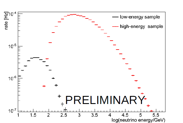
Figure 1: Distribution of the neutrino energy of atmospheric neutrinos in the low-energy (DeepCore) and in the high-energy (IceCube) sample.

We extracted two samples of upwards going neutrino events from data collected by IceCube-79, one at relatively high energies using data from the entire IceCube detector and one at lower energies selected in the DeepCore volume, rejecting backgrounds by an active veto [4]. Neutrino oscillations are expected to affect only the low-energy sample. The high-energy sample provided large statistics outside the signal region and served to constrain systematic uncertainties.

The directions of the muon tracks in the high-energy sample were reconstructed with the standard maximum likelihood muon track in IceCube [5]. For low-energy events, the same method was applied as an initial step. As the hypothesis of a throughgoing track is not correct for these, the finiteness of the tracks was considered in a second step. The track length and the start/stop points of the track were determined as well as the likelihood whether the track is starting and/or stopping in the detector [4]. Quality cuts like the number of unscattered photons and the track likelihood allowed for the rejection of misreconstructed downwards going muon background.

In Fig. 1, the neutrino energy distribution of the low-energy and the high-energy sample are shown. The resolution of the reconstructed zenith angle is essential because the propagation length is proportional to cos(zenith). A variation of the zenith thus represents a variation of L/E. As displayed in Fig. 2, a resolution of $8^{\circ}$ is achieved for the low-energy sample, independent from the zenith.

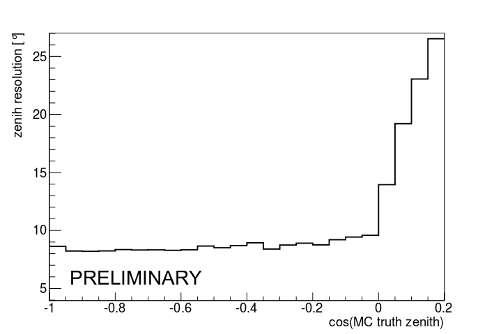
Figure 2: Zenith resolution (mean absolute difference between true and reconstructed track) for the low-energy sample as a function of true zenith.

A modified version of the atmospheric neutrino flux model derived by Honda et al. [6] was used because recent measurements of the spectrum of charged cosmic rays in the energy range of 200 GeV to 100 TeV indicate a cosmic ray spectrum flatter than that assumed by Honda et al., see e.g. [7]. We adjusted the resulting neutrino spectrum by hardening its spectral index by 0.05 to reflect these new measurements.

3 Systematic uncertainties

A covariance matrix in a $\chi^{2}$ fit was used to consider systematic uncertainties in the data analysis. In order to obtain the most likely value of the individual sources of systematic errors, the pulls as defined in [8] were used. The following sources of systematic uncertainties were considered explicitly and propagated by Monte Carlo (MC) simulation to the final selection level:

• the absolute sensitivity of the IceCube sensors ($\pm 10\%)$ and the relative efficiency of the more efficient DeepCore sensors ($1.35\pm 0.03$)

• the optical parameters (scattering, absorption) of the ice as detector medium: the uncertainty is estimated by the difference of the optical parameters obtained by the extraction methods [9] and [10]

• the absolute normalization of the cosmic ray flux ($\pm 25\%$) and its spectral index ($\pm 0.05$)

• the uncertainty of the neutrino production rate in the atmosphere: the difference of calculations by [6] and [11] were used for $\nu_{\mu}$ and for $\nu_{e}$.

4 Results

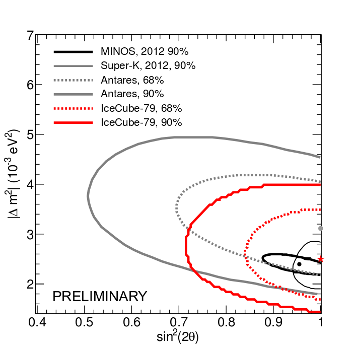
Figure 3: $68\%$ and $90\%$ CL contour line of the result of the IceCube-79 oscillation analysis in comparison with the results of Antares[12], Minos and SuperKamiokande[13].

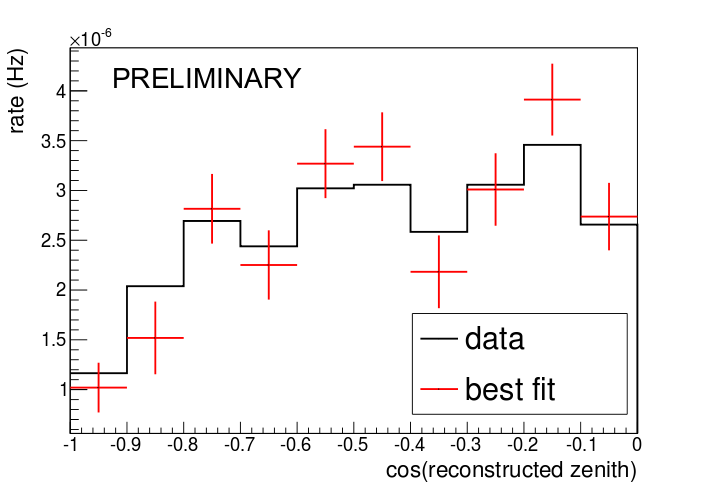
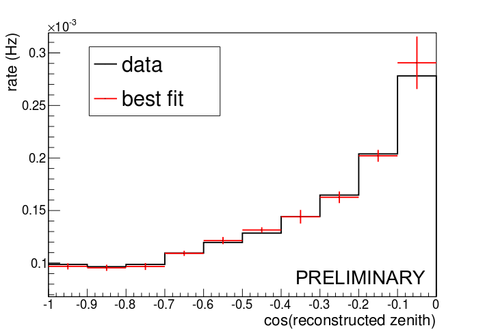
Figure 4: Data and MC expectation at best fit (physics parameters and pulls) in the low energy sample and for the high energy sample.

During May 2010 to May 2011, we collected $318.9$ days of high quality data, excluding periods of calibration runs, partial detector configurations and detector downtime. The low energy sample contained 719 events, while the high energy sample contained $39,638$ events after final cuts. In a first step, we evaluated the $\chi^{2}$ for the data collected by IceCube for two different physics hypotheses: the standard oscillation scenario represented by the world average best fit parameters and the non-oscillation case. With $\Delta\chi^{2}=30$, we rejected the non-oscillation hypothesis with a p-value of $10^{-8}$, corresponding to $5.6\sigma$. The significance was evaluated by a toy MC considering deviations from a $\chi^{2}$ distribution (both hypotheses do not correspond to the minimum $\chi^{2}$).

In a second step, the $\chi^{2}$ was evaluated as a function of the oscillation parameters. The best fit is given by $\Delta m^{2}_{23}=2.5\cdot 10^{-3}$eV$\texttwosuperior$ and $\sin^{2}2\theta_{23}=1$, with an absolute $\chi^{2}=11.3$ and 18 degrees of freedom (20 bins, 2 fitted parameters). The value of the absolute $\chi^{2}$ corresponds to a goodness-of-fit p-value of $0.88$. This indicates a good agreement of data to MC within the assumed uncertainties. All pulls on the systematic uncertainties are within the $1\sigma$ uncertainty range. The data as a function of zenith together with the statistical $1\sigma$ range of the MC expectation corrected for the pulls is shown in Fig. 4. The result is in good agreement with other experiments, which measured the atmospheric oscillations with a high resolution at lower energies[13].

The two dimensional confidence regions of the oscillation parameters in this measurement were determined from the $\Delta\chi^{2}$ around the best fit with two degrees of freedom ($68\%$ CL: $\Delta\chi^{2}=2.30$ and $90\%$ CL: $\Delta\chi^{2}=4.61$), see Fig. 3. The confidence regions of the individual parameters were determined by marginalization analogous to a profile likelihood method. We obtain $68\%$ CL intervals of $\Delta m^{2}_{23}=(2.5\pm 0.6)\cdot 10^{-3}$ eV² and $\sin^{2}2\theta_{23}>0.92$ using $\Delta\chi^{2}$ with one degree of freedom.

The analysis of IceCube data presented here provided the first significant detection of atmospheric neutrino oscillations with a high-energy neutrino telescope. In future, a significant improvement of the resolution of IceCube on the atmospheric neutrino oscillations is expected by the inclusion of the reconstructed neutrino energy in the analysis, by the use of new reconstruction methods which are more efficient at lower energies and by the inclusion of two additional dedicated DeepCore strings which started data taking in May 2011.

References

- [1] J. Beringer, et al., Phys.Rev. D86 (2012) 010001.
- [2] R. Abbasi, et al., Astropart.Phys. 35 (2012) 615–624.
- [3] A. Achterberg, et al., Astropart.Phys. 26 (2006) 155–173.
- [4] O. Schulz, S. Euler, D. Grant, et al., Proceedings of the 31st ICRC, Lodz, Poland (2009) contribution 1237.
- [5] J. Ahrens, et al., Nucl.Instrum.Meth. A524 (2004) 169–194.
- [6] M. Honda, T. Kajita, K. Kasahara, S. Midorikawa, T. Sanuki, Phys.Rev. D75 (2007) 043006.
- [7] Y. Yoon, H. Ahn, P. Allison, M. Bagliesi, J. Beatty, et al., Astrophys.J. 728 (2011) 122.
- [8] G. Fogli, E. Lisi, A. Marrone, D. Montanino, A. Palazzo, Phys.Rev. D66 (2002) 053010.
- [9] M. Ackermann, et al., J. Geophys. Res. 111 D13203.
- [10] D. Chirkin, et al., Proceedings of the 32nd ICRC, Beijing, China (2011), contribution 333.
- [11] G. Barr, S. Robbins, T. Gaisser, T. Stanev, P. Lipari (2003) 1411–1414.
- [12] S. Adrian-Martinez, et al., Phys.Lett. B714 (2012) 224–230.
- [13] http://www numi.fnal.gov/PublicInfo/forscientists.html.
- [14] F. An, et al., Phys.Rev.Lett. 108 (2012) 171803.
- [15] J. Ahn, et al., Phys.Rev.Lett. 108 (2012) 191802.
- [16] R. Abbasi, et al., Phys.Rev. D84 (2011) 082001.
- [17] R. Abbasi, et al., Nucl.Instrum.Meth. A618 (2010) 139–152.