Localized states in the conserved Swift-Hohenberg equation with cubic nonlinearity

Abstract

The conserved Swift-Hohenberg equation with cubic nonlinearity provides the simplest microscopic description of the thermodynamic transition from a fluid state to a crystalline state. The resulting phase field crystal model describes a variety of spatially localized structures, in addition to different spatially extended periodic structures. The location of these structures in the temperature versus mean order parameter plane is determined using a combination of numerical continuation in one dimension and direct numerical simulation in two and three dimensions. Localized states are found in the region of thermodynamic coexistence between the homogeneous and structured phases, and may lie outside of the binodal for these states. The results are related to the phenomenon of slanted snaking but take the form of standard homoclinic snaking when the mean order parameter is plotted as a function of the chemical potential, and are expected to carry over to related models with a conserved order parameter.

I Introduction

Spatially localized structures (hereafter LS) are observed in a great variety of pattern-forming systems. Such states include spot-like structures found in reaction-diffusion systems CRT00 and in a liquid light-valve experiment BCR09 , isolated spikes observed in a ferrofluid experiment RB05 and localized buckled states resulting from the buckling of slender structures under compression HPCWWBL00 . Related states are observed in fluid mechanics, including convection bkam06 ; BK:08b ; Blanchflower99 and shear flows sgb10 . In other systems, such as Faraday waves, the LS oscillate in time, either periodically or with a more complex time-dependence, forming structures referred to as oscillons laf96 ; rlc11 . This is also the case for oscillons in granular media UMS:96 and in optics AFO09 . Other examples of LS include localized traveling waves Kolodner88 ; Barten91 and states called “worms” observed in electroconvection Dennin96 ; Riecke98 . In many of these systems the use of envelope equations removes the (fast) time-dependence and maps such time-dependent structures onto equilibria.

Many of the structures mentioned above are examples of “dissipative solitons” PBA10 in which energy loss through dissipation is balanced by energy input through spatially homogeneous forcing. Others (e.g., RB05 ; HPCWWBL00 ) correspond to local minima of an underlying energy or Lyapunov functional. This is the case for systems whose dynamics are of gradient type, provided only that the energy is bounded from below. On finite domains with null boundary conditions such systems evolve to steady states which may or may not correspond to LS. However, in generic systems supporting dissipative solitons no Lyapunov function will be present and the evolution of the system may be nonmonotonic.

In either system type, time-independent LS are found in regions of parameter space in which a time-independent spatially homogeneous (i.e., uniform) state coexists with a time-independent spatially periodic state. Within this region there is a subregion referred to as the snaking or pinning region Pom:86 in which a great variety of stationary LS are present. In the simplest, one-dimensional, case the LS consist of a segment of the periodic state embedded in a homogeneous background; segments of the homogeneous state embedded in periodic background may be thought of as localized hole states LH. Steady states of this type lie on a pair of intertwined branches that snake back and forth across the snaking region, one of which consists of reflection-symmetric LS with a peak in the center, while the other consists of similar states but with a dip in the center, and likewise for the holes. Near the left edge of the snaking region each LS adds a pair of new cells, one at either end, and these grow to full strength as one follows the LS across the snaking region to its right edge, where both branches turn around and the process repeats. Thus, as one follows the LS branches towards larger $L^{2}$ norm, both types of LS gradually grow in length, and all such structures coexist within the snaking region. On a finite interval the long LS take the form of holes in an otherwise spatially periodic state but on the real line, the LS and LH remain distinct although both occupy the same snaking region. The LS branches are, in adition, interconnected by cross-links resembling the rungs of a ladder, consisting of asymmetric LS bukn07 . In generic systems posed on the real line states of this type drift, either to the left or the right, depending on the asymmetry, but in systems with gradient dynamics the asymmetric states are also time-independent. These, along with bound states of two, three, etc LS/LH are also present within the snaking region bukn07 .

The above behavior is typical of nonconserved order parameter fields. However, an important subclass of gradient systems possesses a conserved quantity, and in such systems the order parameter field has a fixed mean value. Systems of this type arise frequently in fluid convection and other applications CM01 ; LBK11 ; BBKK12 and are distinguished from the standard scenario summarised above by the following properties FCS07 ; dawe08 : (i) the snaking becomes slanted (sometimes referred to as “sidewinding”), (ii) LS may be present outside of the region of coexistence of the homogeneous and periodic states, (iii) LS are present even when the periodic states bifurcate supercritically, i.e., when the coexistence region is absent entirely. The slanting of the snakes-and-ladders structure is a finite size effect: in a finite domain expulsion of the conserved quantity from the LS implies its shortage outside, a fact that progressively delays (to stronger forcing) the formation events whereby the LS grow in length. The net effect is that LS are found in a much broader region of parameter space than in nonconserved systems.

The above properties are shared by many of the models arising in dynamical density functional theory (DDFT) and related phase field models of crystalline solids. The simplest such phase field crystal (PFC) model PFC_review (see below) leads to the so-called conserved Swift-Hohenberg (cSH) equation. This equation was first derived, to the authors’ knowledge, as the equation governing the evolution of binary fluid convection between thermally insulating boundary conditions K:89 ; for recent derivations in the PFC context see Refs. vBVL09 ; ARTK12 ; PFC_review . In this connection the PFC model may be viewed as probably the simplest microscopic model for the freezing transition that can be constructed. In this model the transition from a homogeneous state to a periodic state corresponds to the transition from a uniform density liquid to a periodic crystalline solid. The LS of interest in this model then correspond to states in which a finite size portion of the periodic crystalline phase coexists with the uniform density liquid phase, and these are expected to be present in the coexistence region between the two phases. Some rather striking examples of LS in large two-dimensional systems include snow-flake-like and dendritic structures, e.g., Refs. PFC_review ; tegz09 ; tegz09b ; tegz09c ; tams08 . In fact, as shown below, the LS are also present at state points outside of the coexistence region. However, despite the application of the cSH (or PFC) equation in this and other areas, the detailed properties of the LS described by this equation have not been investigated. In this paper we make a detailed study of the properties of this equation in one spatial dimension with the aim of setting this equation firmly in the body of literature dealing with spatially localized structures. Our results are therefore interpreted within both languages, in an attempt to make existing understanding of LS accessible to those working on nonequilibrium models of solids, and to use the simplest PFC model to exemplify the theory. In addition, motivated by Refs. tegz09 ; tegz09b ; tegz09c ; tams08 , we also describe related results in two (2d) and three (3d) dimensions, where (many) more types of regular patterns are present and hence many more types of LS. Our work focuses on ‘bump’ states (also referred to as ‘spots’) which are readily found in direct numerical simulations of the conserved Swift-Hohenberg equation as well as in other systems BCR09 .

Although the theory for these cases in 2d and 3d is less well developed LSAC08 ; ALBKS10 continuation results indicate that some of the various different types of LS can have quite different properties. For example, the bump states differ from the target-like LS formed from the stripe state that can also be seen in the model. In particular, spots in the nonconserved Swift-Hohenberg equation in the plane bifurcate from the homogeneous state regardless of whether stripes are subcritical or supercritical LS09 , see also Ref. MS10 . The key question, hitherto unanswered, is whether two-dimensional structures in the plane snake indefinitely and likewise for three-dimensional structures.

The paper is organized as follows. In Sec. II we describe the conserved Swift-Hohenberg equation and its basic properties. In Sec. III we describe the properties of LS in one spatial dimension as determined by numerical continuation. In Sec. IV we describe related results in two and three spatial dimensions, but obtained by direct numerical simulation of the PFC model. Since this model has a gradient structure, on a finite domain all solutions necessarily approach a time-independent equilibrium. However, as we shall see, the number of competing equilibria may be very large and different equilibria are reached depending on the initial conditions employed. In Sec. V we put our results into context and present brief conclusions.

II The conserved Swift-Hohenberg equation

II.1 Equation and its variants

We write the cSH (or PFC) equation in the form

$$\partial_{t}\phi(\mathbf{x},t)=\alpha\nabla^{2}\frac{\delta F[\phi]}{\delta\phi(\mathbf{x},t)},$$ (1)

where $\phi(\mathbf{x},t)$ is an order parameter field that corresponds in the PFC context to a scaled density profile, $\alpha$ is a (constant) mobility coefficient and $F[\phi]$ denotes the free energy functional

$$F[\phi]\equiv\int d\mathbf{x}\left[\frac{\phi}{2}[r+(q^{2}+\nabla^{2})^{2}]\phi+\frac{\phi^{4}}{4}\right].$$ (2)

Here $\mathbf{x}=(x,y,z)$, $\nabla=(\partial_{x},\partial_{y},\partial_{z})^{T}$ is the gradient operator, and subscripts denote partial derivatives. It follows that the system evolves according to the cSH equation

$$\partial_{t}\,\phi\,=\,\alpha\nabla^{2}\left[r\phi+(\nabla^{2}+q^{2})^{2}\phi+\phi^{3}\right].$$ (3)

Equation (3) is sometimes called the derivative Swift-Hohenberg equation MaCo00 ; Cox04 ; many papers use a different sign convention for the parameter $r$ (e.g., EKHG02 ; Achi09 ; GDL09 ; SHP06 ; BRV07 ; OhSh08 ; MKP08 ; tegz09 ; vBVL09 ). In this equation the quartic term in $F[\phi]$ may be replaced by other types of nonlinearity, such as $f_{23}=-b_{2}\phi^{3}/3+\phi^{4}/4$ MaCo00 ; Cox04 ; tegz09 ; vBVL09 without substantial change in behavior. Related but nonconserved equations $\partial_{t}\phi=-\tilde{\alpha}\delta F[\phi]/\delta\phi$ with nonlinear terms of the form $f_{23}$ BuKn06 or $f_{35}=-b_{3}\phi^{4}/4+\phi^{6}/6$ bukn07 have also been extensively studied, subject to the conditions $b_{2}>27/38$ (resp., $b_{3}>0$) required to guarantee the presence of an interval of coexistence between the homogeneous state $\phi=0$ and a spatially periodic state. Note that in the context of nonconserved dynamics BuKn06 ; bukn07 one generally selects a nonlinear term $g_{\mathrm{nl}}$ directly, although this term is related to $f_{\mathrm{nl}}$ through the relation $g_{\mathrm{nl}}\equiv-df_{\mathrm{nl}}/d\phi$, i.e., $g_{23}$ or $g_{35}$. As we shall see below, in the conserved case, having the nonlinear term $f_{23}$ describes the generic case and the role of the coefficient $b_{2}$ is effectively played by the value of $\phi_{0}$, which is the average value of the order parameter $\phi(\mathbf{x})$.

Equation (3) can be studied in one, two or more dimensions. In one dimension with $g_{23}$ the equation was studied by Matthews and Cox MaCo00 ; Cox04 as an example of a system with a conserved order parameter; this equation is equivalent to Eq. (3) with imposed nonzero mean $\phi$. A weakly localized state of the type that is of interest in the present paper is computed in MaCo00 and discussed further in Cox04 .

II.2 Localized states in one spatial dimension

We first consider Eq. (3) in one dimension, with $\alpha=1$ and $q=1$, i.e.,

$$\partial_{t}\,\phi\,=\,\partial^{2}_{x}\left[r\phi+(\partial^{2}_{x}+1)^{2}\phi+\phi^{3}\right].$$ (4)

This equation is reversible in space (i.e., it is invariant under $x\rightarrow-x$). Moreover, it conserves the total “mass” $\int_{0}^{L}\phi\,dx$, where $L$ is the size of the system. In the following we denote the average value of $\phi$ in the system by $\phi_{0}\equiv\langle\phi\rangle$ so that perturbations ${\tilde{\phi}}\equiv\phi-\phi_{0}$ necessarily satisfy $\langle{\tilde{\phi}}\rangle=0$, where $\langle\cdots\rangle\equiv L^{-1}\int_{0}^{L}(\cdots)\,dx$.

Steady states ($\partial_{t}\,\phi\,=\,0$) are solutions of the fourth order ordinary differential equation

$$0=r\phi+(\partial_{xx}+1)^{2}\phi+\phi^{3}-\mu,$$ (5)

where $\mu\equiv\delta F[\phi]/\delta\phi$ is an integration constant that corresponds to the chemical potential.

Each solution of this equation corresponds to a stationary value of the underlying Helmholtz free energy

$$\tilde{F}=\int_{0}^{L}\left[(1+r)\frac{\phi^{2}}{2}+\frac{\phi^{4}}{4}-(\partial_{x}\phi)^{2}+\frac{1}{2}(\partial_{xx}\phi)^{2}\right]\,dx.$$ (6)

We use the free energy to define the grand potential

$$\Omega=\tilde{F}-\int_{0}^{L}\mu\phi\,dx$$ (7)

and will be interested in the normalized free energy density $f=(\tilde{F}[\phi(x)]-\tilde{F}[\phi_{0}])/L$ and in the density of the grand potential $\omega=\Omega/L=\tilde{F}[\phi(x)]/L-\mu{\phi_{0}}$. We also use the $L^{2}$ norm

$$||\delta{\phi}||=\sqrt{\frac{1}{L}\int_{0}^{L}(\phi-\phi_{0})^{2}\,dx}$$ (8)

as a convenient measure of the amplitude of the departure of the solution from the homogeneous background state $\phi=\phi_{0}$.

Linearizing Eq. (4) about the steady homogeneous solution $\phi=\phi_{0}$ using the ansatz $\delta\phi(x,t)\equiv\phi(x,t)-\phi_{0}=\epsilon\exp(\beta t+ikx)$ with $\epsilon\ll 1$ results in the dispersion relation

$$\beta=-k^{2}\,[r+(1-k^{2})^{2}+3\phi_{0}^{2}].$$ (9)

It follows that in an infinite domain, the threshold for instability of the homogeneous state corresponds to $r_{c}^{\infty}=-3\phi_{0}^{2}$. In a domain of finite length $L$ with periodic boundary conditions (PBC), the homogeneous state is linearly unstable for $r<r_{n}$, where

$$r_{n}=-(1-k_{n}^{2})^{2}-3\phi_{0}^{2},$$ (10)

and $k_{n}\equiv 2\pi n/L$, $n=1,2,\dots$. Standard bifurcation theory with PBC shows that for $L<\infty$ each $r_{n}$ corresponds to a bifurcation point creating a branch of periodic solutions that is uniquely specified by the corresponding integer $n$. For those integers $n$ for which $r_{n}>-9/2$ the branch of periodic states bifurcates supercritically (i.e., towards smaller values of $|\phi_{0}|$); for $r_{n}<-9/2$, the bifurcation is subcritical (i.e., the branch bifurcates towards larger values of $|\phi_{0}|$). Since each solution can be translated by an arbitrary amount $d$ (mod $L$), each bifurcation is in fact a pitchfork of revolution. Although the periodic states can be computed analytically for $r\approx r_{n}$, for larger values of $|r-r_{n}|$ numerical computations are necessary. In the following we use the continuation toolbox AUTO DKK91 ; AUTO07P to perform these (and other) calculations. For interpreting the results it is helpful to think of $r$ as a temperature-like variable which measures the undercooling of the liquid phase.

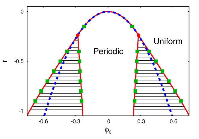
Figure 1: (color online) The phase diagram for the 1d PFC model (3) when $q=1$. The red solid lines are the coexistence curves between the periodic and uniform phases calculated using a two mode approximation ARTK12 . The green squares show the coexistence values calculated from simulations ARTK12 . The red circles are the tricritical points. The blue dashed line shows the curve of marginal stability of the uniform state within linear stability theory.

Before we can discuss LS in the above model, it is helpful to refer to the phase diagram appropriate to a one-dimensional setting (Fig. 1). As shown in Ref. ARTK12 the tricritical point is located at $(\phi_{0b},r_{b}^{\mathrm{max}})=(\pm\sqrt{3/38},-9/38)$. For $r>r_{b}^{\mathrm{max}}$ there exists no thermodynamic coexistence zone between the homogeneous and periodic states. Such a region is only present for $r<r_{b}^{\mathrm{max}}$ and is limited by the binodal lines that indicate the values of $\phi_{0}$ for which the homogeneous and periodic solutions at fixed $r$ have equal chemical potential and pressure (i.e., equal grand potential). Thus for $r<r_{b}^{\mathrm{max}}$ the transition from the homogeneous to the periodic state is of first order. The binodals can either be calculated for specific domain sizes and periods of the periodic structure or for an infinite domain. In the latter case the period of the periodic state is not fixed but corresponds to the period that minimizes the Helmholtz free energy at each $(\phi_{0},r)$ ARTK12 . We remark that with this choice of parameters the tricritical point is not the point at which the bifurcation to the periodic state changes from supercritical to subcritical. As already mentioned, the latter occurs at $(\phi_{0},r)=(\pm\sqrt{3/2},-9/2)$, i.e., at values of $r$ much smaller than $r_{b}^{\mathrm{max}}$. Further discussion of this point may be found in the conclusions.

III Results for the conserved Swift-Hohenberg equation

III.1 Families of localized states

Since Eq. (4) represents conserved gradient dynamics based on an energy functional that allows for a first order phase transition between the homogeneous state and a periodic patterned state, one may expect the existence of localized states (LS) to be the norm rather than an exception. In the region between the binodals, where homogeneous and periodic structures may coexist, the value of $\phi_{0}$, i.e., the amount of ‘mass’ in the system, determines how many peaks can form.

As in other problems of this type we divide the LS into three classes. The first class consists of left-right symmetric structures with a peak in the middle. Structures of this type have an overall odd number of peaks and we shall refer to them as odd states, hereafter LS_odd. The second class consists of left-right symmetric structures with a dip in the middle. Structures of this type have an overall even number of peaks and we refer to them as even states, hereafter LS_even. Both types have even parity with respect to reflection in the center of the structure. The third class consists of states of no fixed parity, i.e., asymmetric states, LS_asym. The asymmetric states are created from the symmetric states at pitchfork bifurcations and take the form of rungs on a ladder-like structure with interconnections between LS_odd to LS_even. In view of the gradient structure of Eq. (4) the asymmetric states are likewise stationary solutions of the equation.

We now address the following questions:
1. Do localized states exist outside the binodal region? Can they form the energetic minimum outside the binodal region?
2. How does the bifurcational structure of the localized states change with changes in the temperature-like parameter $r$? How does the transition from tilted or slanted snaking to no snaking occur? What is the behavior of the asymmetric localized states during this process?

Answers to these and other questions can be obtained by means of an in-depth parametric study. In the figures that follow we present bifurcation diagrams for localized states as a function of the mean order parameter value $\phi_{0}$ for a number of values of the parameter $r$. All are solutions of Eq. (5) that satisfy periodic boundary conditions on the domain $0\leq x\leq L$, and are characterized by their $L^{2}$ norm $||\delta\phi||$, chemical potential $\mu$, free energy density $f$, and grand potential density $\omega$ as defined in Sec. II.2.

In Fig. 2 we show the results for $r=-0.9$ for $L=100$. Figure 2(a) shows $||\delta\phi||$ as a function of $\phi_{0}$: the classical bifurcation diagram. For these parameter values, as $\phi_{0}$ is increased the homogeneous (liquid) phase first becomes unstable to perturbations with mode number $n=16$ (i.e., 16 bumps), followed closely by bifurcations to modes with $n=15$ and $n=17$. All other modes bifurcate at yet smaller values of $|\phi_{0}|$ and are omitted. All three primary bifurcations are supercritical. The figure also reveals that the $n=16$ branch undergoes a secondary instability already at small amplitude; this instability creates a pair of secondary branches of spatially localized states, LS_odd (solid line) and LS_even (dashed line). With increasing amplitude these branches undergo slanted snaking as one would expect on the basis of the results for related systems with a conservation law dawe08 ; LBK11 . The LS_odd and LS_even branches are in turn connected by ladder branches consisting of asymmetric states LS_asym, much as in standard snaking BuKn06 . Sample solution profiles for these three types of LS are shown in Fig. 3. The snaking ceases when the LS have grown to fill the available domain; in the present case the LS_odd and LS_even branches terminate on the same $n=16$ branch that created them in the first place. Whether or not this is the case depends in general on the domain length $L$, as discussed further in Ref. BBKM08 .

The key to the bifurcation diagram shown in Fig. 2(a) is evidently the small amplitude bifurcation on the $n=16$ branch. This bifurcation destabilises the $n=16$ branch that would otherwise be stable and is a consequence of the presence of the conserved quantity $\phi_{0}$ MaCo00 . As $L$ increases, the bifurcation moves down to smaller and smaller amplitude, so that in the limit $L\rightarrow\infty$ the periodic branch is entirely unstable and the LS bifurcate directly from the homogeneous state. Since the LS bifurcate subcritically it follows that such states are present not only when the primary pattern-forming branch is supercritical but moreover are present below the onset of the primary instability.

Figure 2(b) shows the corresponding plot of the free energy density $f$ as a function of $\phi_{0}$. This figure demonstrates that throughout much of the range of $\phi_{0}$ the localized states have a lower free energy than the extended periodic states. In this range the LS are therefore energetically favored. Figure 2(c) shows the corresponding plot of the chemical potential $\mu$ while Fig. 2(d) shows the grand potential density $\omega$. Of these Fig. 2(c) is perhaps the most interesting since it shows that the results of Fig. 2(a), when replotted using $(\phi_{0},\mu)$ to characterize the solutions, in fact take the form of standard snaking, provided one takes the chemical potential $\mu$ as the control parameter and $\phi_{0}$ as the response. In this form the bifurcation diagram gives the values of $\phi_{0}$ that are consistent with a given value of the chemical potential $\mu$ (recall that $\phi_{0}$ is related to the total particle number density).

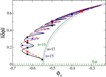
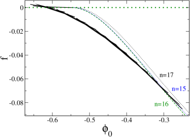
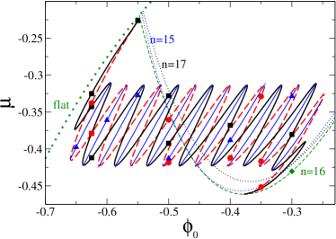
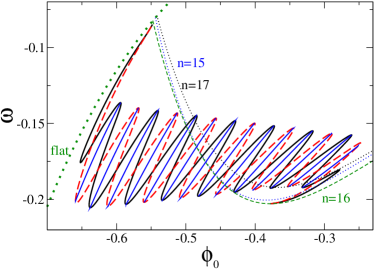
(a) (b) (c) (d)

Figure 2: (color online) Characteristics of steady state (localized) solutions of the one-dimensional conserved Swift-Hohenberg equation (4) as a function of the mean order parameter $\phi_{0}$ for a fixed domain size of $L=100$ and $r=-0.9$. The various solution profiles are characterized by their (a) $L^{2}$ norm $||\delta\phi||$, (b) free energy density $f$, (c) chemical potential $\mu$, and (d) grand potential density $\omega$. The thick green dotted line, labeled ‘flat’, corresponds to the homogeneous solution $\phi(x)=\phi_{0}$. Periodic solutions with $n=16$ peaks are shown as a thin green dashed line, whereas the nearby thin blue and black dotted lines represent the $n=15$ and $n=17$ solutions, respectively. The thick solid black and dashed red lines that bifurcate from the $n=16$ periodic solution represent symmetric localized states with a maximum (LS_odd) and a minimum (LS_even) at their center, respectively. Both terminate on the $n=16$ solution. The 14 blue solid lines that connect the LS_odd and LS_even branches of symmetric localized states correspond to asymmetric localized states (LS_asym). Together these three sets of branches of localized states form a tilted snakes-and-ladders structure. Typical order parameter profiles along the three LS branches are shown in Fig. 3, and correspond to locations indicated in panels (a) and (c) by filled black squares (LS_odd), red circles (LS_even), blue triangles (LS_asym) and green diamond (periodic solution with $n=16$).

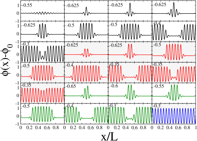
Figure 3: (Color online) A selection of steady state profiles $\phi(x)-\phi_{0}$ for $r=-0.9$ and values of $\phi_{0}$ in the range $-0.65\leq\phi_{0}\leq-0.3$ (the number in each panel indicates the corresponding value of ${\phi}_{0}$). Going from top left to bottom right we first show nine LS_odd solutions, i.e., symmetric localized states with an odd number of maxima (in black), then eight LS_even solutions, i.e., symmetric localized states with an even number of maxima (in red), followed by six LS_asym solutions, i.e., asymmetric localized states (in green). The final plot is the $n=16$ periodic solution for ${\phi}_{0}=-0.3$ (in blue). The solutions on the symmetric branches correspond to locations indicated in Fig. 2(a) and are shown in order, starting from the bifurcation point that creates them and continuing to larger norm $||\delta\phi||$. The color coding corresponds to that used in Figs. 2(a,c): LS_odd (filled black squares), LS_even (red circles), LS_asym (blue triangles) and periodic (green diamond).

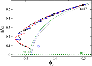
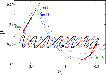
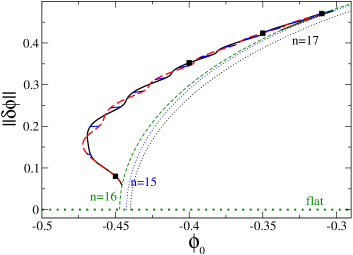
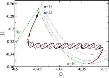
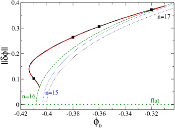
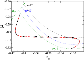
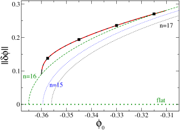
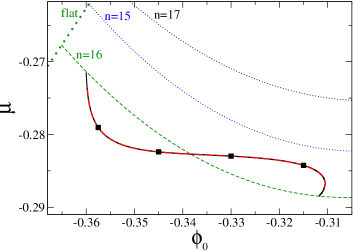
(a) (b) (c) (d) (e) (f) (g) (h)

Figure 4: (color online) The norm (left) and chemical potential (right) of the homogeneous, periodic and localized steady state solutions as a function of the mean order parameter $\phi_{0}$, for a fixed domain size of $L=100$ and several values of $r>-0.9$. In (a,b) $r=-0.7$, (c,d) $r=-0.6$, (e,f) $r=-0.5$, and (g,h) $r=-0.4$. The line styles are as in Fig. 2. Typical order parameter profiles along the branches of symmetric localized states with an odd number of maxima (black lines) are shown in Fig. 5, and correspond to locations indicated in the panels by filled black squares.

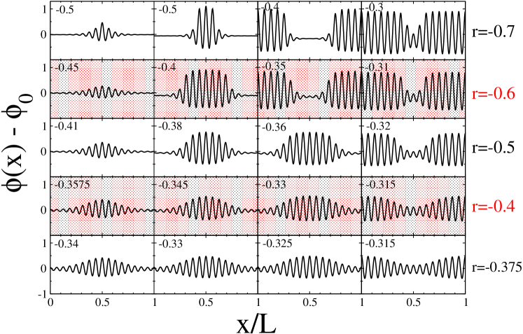
Figure 5: (Color online) A selection of steady state profiles $\phi(x)-\phi_{0}$ along the LS_odd branches shown in Fig. 4 for $r=-0.7$ (1st row), $r=-0.6$ (2nd row), $r=-0.5$ (3rd row), $r=-0.4$ (4th row), and $r=-0.375$ (last row), for various values of ${\phi}_{0}$, as indicated in the top left corner of each panel. The solutions in each row are shown in order, starting from near the bifurcation point that creates them and continuing to larger norm $||\delta\phi||$. The locations of the profiles are indicated in Fig. 4 by the filled black squares. The bifurcation diagram for $r=-0.375$ (not shown in Fig. 4) is qualitatively the same as that for $r=-0.4$.

We now show how the bifurcation diagrams evolve as the temperature-like parameter $r$ changes. We begin by showing the bifurcation diagrams for decreasing values of $|r|$. In the Appendix we use amplitude equations to determine the direction of branching of the localized states. Here we discuss the continuation results.

The bifurcation diagram for $r=-0.7$ (Fig. 4(a,b)) resembles that for $r=-0.9$ (Fig. 2) although the snaking structure has moved towards smaller $|\phi_{0}|$ and is now thinner. In addition, it is now the second saddle-node on the LS_odd branch that lies farthest to the left, and not the first. For $r=-0.6$ (Fig. 4(c,d)), the branches of localized states still form a tilted snakes-and-ladders structure, but the saddle-nodes on the LS_odd and LS_even branches are now absent, i.e., both solution branches now grow monotonically. The resulting diagram has been called “smooth snaking” DL10 . However, despite the absence of the saddle-nodes on the LS_odd and LS_even branches the interconnecting ladder states consisting of asymmetric states still remain. This continues to be the case when $r=-0.5$ (Fig. 4(e,f)) although the structure has moved to yet larger $\phi_{0}$ and the snake has become even thinner. Finally, for $r=-0.4$ (Fig. 4(g,h)), the snake is nearly dead, and only tiny wiggles remain. The bifurcation of the localized states from the $n=16$ periodic state is now supercritical (see Appendix) but the LS branches continue to terminate on the same branch at larger amplitude, and do so via a single saddle-node at the right (Fig. 4(h)). Sample profiles along the resulting LS_odd branches are shown for several values of $r$ in Fig. 5. We note that a change of $r$ has a profound effect on the transition region between the homogeneous background state and the periodic state: with decreasing $|r|$ the LS become wider and the localized periodic structure looks more and more like a wave packet with a smooth sinusoidal modulation of the peak amplitude.

As the ‘temperature’ $r$ decreases even further, the bifurcation diagrams remain similar to those displayed in Fig. 2 until just before $r=-1.5$, where substantial changes take place and the complexity of the bifurcation diagram grows dramatically. This is a consequence of the appearance of other types of localized states that we do not discuss here. Likewise, we omit here all bound states of the LS described above. These are normally found on an infinite stack of isolas that are also present in the snaking region bukn09 ; KLSW:11 .

III.2 Tracking the snake

In Fig. 6 we show, for $-1.5<r<-0.4$, the result of tracking all the saddle-node bifurcations visible in the previous bifurcation diagrams in the $(\phi_{0},r)$ plane, while Fig. 7 shows an enlargement of the region $-1<r<-0.35$ together with the result of tracking the tertiary pitchfork bifurcations to the asymmetric states.

Figure 6 shows that the saddle-nodes annihilate pairwise in cusps as $r$ increases. The annihilations occur first for smaller $\phi_{0}$ and later for larger $\phi_{0}$, and occur alternately on LS_odd and LS_even. Above the locus of the cusps the snaking is smooth, although as shown in Fig. 7 the tertiary ladder states remain. The thick green curve in Fig. 7 represents the locus of the secondary bifurcation from the $n=16$ periodic state to LS and shows that on either side the bifurcation to LS is subcritical for sufficiently negative $r$ but becomes supercritical at larger $r$, cf. Fig. 4(h) and Appendix.

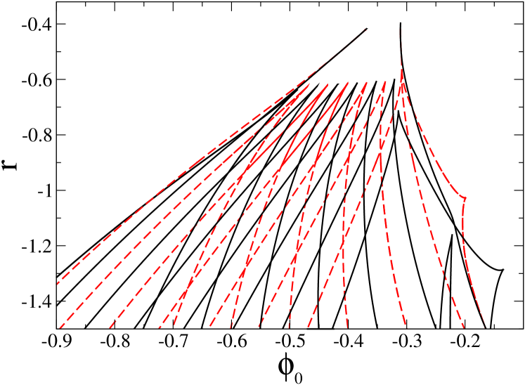
Figure 6: (color online) Loci of saddle-node bifurcations on the branches of symmetric localized states in the $(\phi_{0},r)$ plane for $r>-1.5$. Saddle-nodes annihilate pairwise as $r$ increases (solid black lines: LS_odd; dashed red lines: LS_even).

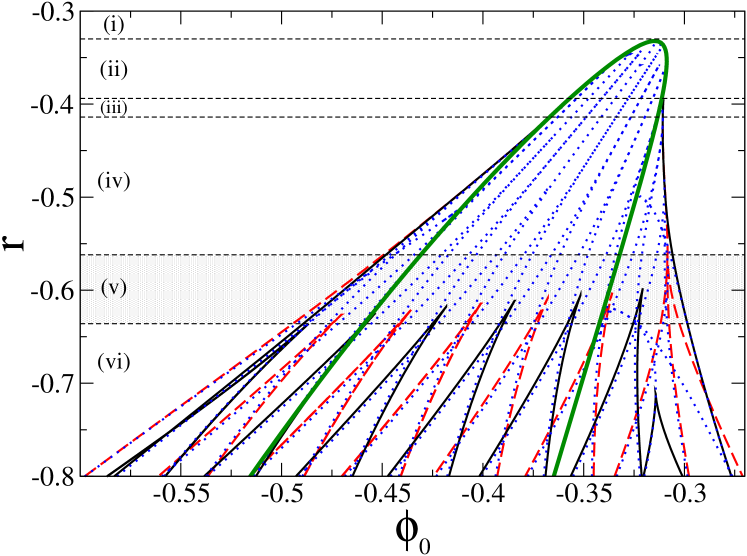
Figure 7: (color online) Loci of the saddle-node bifurcations on the branches of symmetric localized states in the $(\phi_{0},r)$ plane (solid black lines: LS_odd; dashed red lines: LS_even) together with the bifurcations to asymmetric localized states (dotted blue lines) for $r>-1.5$. The thick green curve represents the locus of secondary bifurcation from the periodic $n=16$ state to localized states and shows that on either side the bifurcation to LS is subcritical for sufficiently negative $r$ but becomes supercritical at larger $r$.

One may distinguish six intervals in $r$ with different types of behavior. These depend on the system size, but the results in Fig. 7 for $L=100$ are representative:

• For $r>-0.33$: no LS exist, the only nontrivial states are periodic solutions.

• For $-0.33>r>-0.39$: branches of even and odd symmetric LS are present, and appear and disappear via supercritical secondary bifurcations from the branch of periodic solutions. With decreasing $r$, more and more branches of asymmetric LS emerge from these two secondary bifurcation points.

• For $-0.39>r>-0.41$: both branches of symmetric LS emerge subcritically at large $\phi_{0}$ and supercritically at small $\phi_{0}$.

• For $-0.41>r>-0.56$: both branches of symmetric LS emerge subcritically at either end. Further branches of asymmetric LS emerge with decreasing $r$ either from the two secondary bifurcation points or from the saddle-node bifurcations on the branches of symmetric LS, but the symmetric LS still do not exhibit snaking, i.e., no additional folds are present on the branches of symmetric LS.

• For $-0.56>r>-0.64$ (highlighted by the grey shading in Fig. 7): pairs of saddle-nodes appear successively in cusps as $r$ decreases, starting at larger $\phi_{0}$. Thereafter saddle-nodes appear alternately on branches of even and odd symmetric LS. The appearance of the cusps is therefore associated with the transition from smooth snaking to slanted snaking.

• For $-0.64>r$: The slanted snake is fully developed. Only one further pair of saddle-node bifurcations appears in the parameter region shown in Fig. 7. With decreasing $r$ the snaking becomes stronger; each line in Figs. 6 and 7 that represents a saddle-node bifurcation crosses more and more other such lines, i.e., more and more different states are possible at the same values of $\phi_{0}$. Furthermore, the subcritical regions (outside the green curve in Fig. 7) become larger.

III.3 Relation to binodal lines

From the condensed matter point of view, where the cSH/PFC equation represents a model for the liquid (homogeneous) and solid (periodic) phases, one is particularly interested in results in the thermodynamic limit $L\to\infty$. As mentioned above in the context of the phase diagram in Fig. 1, the binodal lines correspond to values of $(\phi_{0},r)$ at which the homogeneous state and the minimum energy periodic state coexist in the thermodynamic limit. These are defined as pairs of points at which the homogeneous state and the periodic state have the same ‘temperature’ (i.e., same $r$ value), the same chemical potential $\mu$ and the same pressure $p=-\omega$, and are displayed as the blue dash-dot lines in Fig. 8. For a given value of $r$, these two lines give the values of $\phi_{0}$ of the coexisting homogeneous (lower $\phi_{0}$) and periodic (higher $\phi_{0}$) states. Note that when plotted with the resolution of Fig. 8, the binodals are indistinguishable from the coexistence lines between the finite size $L=100$, $n=16$ periodic solution and the homogeneous state. Figure 8 also displays the line (green solid line) at which the $L=100$ localized states bifurcate from the $n=16$ branch of periodic solutions. For $r<-0.4$ the LS bifurcations are subcritical implying that the localized states are present outside the green solid line. Figure 8 shows the loci of the outermost saddle-node bifurcations on the branches of symmetric LS that result (dashed lines to the left and to the right of the green solid line for $r<-0.4$). The most striking aspect of Fig. 8 is that for $r\lesssim-1$ these lines actually cross and exit the region between the two binodal lines, indicating that in the PFC model one can find stable LS outside of the binodal. Although these are not the lowest free energy states (we have checked this for $r\gtrsim-1.5$), this remarkable fact points towards the possibility of metastable nanocrystals existing outside of the binodal. We must mention, however, that these structures have been found in a finite size system with $L=100$; we have not investigated their properties for larger system sizes $L$.

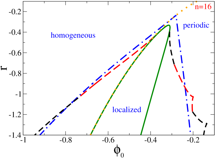
Figure 8: (color online) Loci in the $(\phi_{0},r)$ plane computed for $L=100$ of (i) the primary bifurcation from the homogeneous state to the $n=16$ periodic branch (dotted orange line); (ii) the bifurcation of the localized states from the $n=16$ periodic branch (solid green line); (iii) the outermost saddle-node bifurcations on the branches of symmetric localized states (long-dashed red and short-dashed black lines); and (iv) the binodals between the periodic and homogeneous states (dot-dashed blue lines). The latter coincide with the binodals for the $n=16$ periodic state and the homogeneous state to within the resolution of the figure. Figures 6 and 7 show how the loci of the outermost saddle-node bifurcations of localized states fit into the overall picture.

III.4 Stability

Although we have not computed the stability properties of the different localized states with respect to infinitesimal perturbations, we can use the principles of bifurcation theory to deduce the likely stability properties. In the reference bifurcation diagram in Fig. 2(a) the homogeneous state (liquid) is stable for large negative $\phi_{0}$, and for a system with $L=100$ loses stability to the $n=16$ mode as $\phi_{0}$ increases. Since the bifurcation is supercritical, the $n=16$ periodic state is initially stable. The LS that bifurcate from it subcritically will both be unstable. The single bump state is likely to be once unstable and it therefore acquires stability at the first saddle-node on the left, remaining stable until the first crosslink where a second (phase) eigenvalue becomes unstable. The first (amplitude) eigenvalue becomes unstable at the saddle-node on the right so that the portion of LS_odd with negative slope is twice unstable. These instabilities are then undone so that the LS_odd above the second crosslink are again stable. The transition to smooth snaking that occurs with decreasing $r$ eliminates instabilities associated with the first eigenvalue but not the second.

The LS_even states are initially twice unstable but both eigenvalues stabilize near the first saddle-node on the left, so that LS_even is stable on the part of the branch with positive slope, below the second crosslink etc. Thus the connecting LS_asym are unstable. Once again, the transition to smooth snaking that occurs with decreasing $r$ eliminates instabilities associated with the amplitude eigenvalue but not those associated with the phase eigenvalue. One can check that in this case the connecting LS_asym remain unstable with the LS_odd stable between the second and third crosslinks (Fig. 4(c)), and unstable between the third and fourth crosslinks. Likewise the LS_even are stable above the left saddle-node and below the second crosslink; they are unstable between the second and third crosslinks and acquire stability at the third crosslink etc (Fig. 4(c)). Note that as a result of these stability assignments there is at least one LS state that is stable at all $\phi_{0}$ values between the leftmost and rightmost saddle-nodes.

IV Localized states in two and three dimensions

IV.1 Numerical algorithm

To perform direct numerical simulations (DNS) of the conserved Swift-Hohenberg equation in higher dimensions we use a recently proposed algorithm GoNo12 that has been proved to be unconditionally energy-stable. As a consequence, the algorithm produces free-energy-decreasing discrete solutions, irrespective of the time step and the mesh size, thereby respecting the thermodynamics of the model even for coarse discretizations. For the spatial discretization we employ Isogeometric Analysis HCB05 , which is a generalization of the Finite Element Method. The key idea behind Isogeometric Analysis is the use of Non-Uniform Rational B-Splines (NURBS) instead of the standard piecewise polynomials used in the Finite Element Method. With NURBS Isogeometric Analysis gains several advantages over the Finite Element Method. In the context of the conserved Swift-Hohenberg equation, the most relevant one is that the Isogeometric Analysis permits the generation of arbitrarily smooth basis functions that lead to a straightforward discretization of the higher-order partial derivatives of the conserved Swift-Hohenberg equation GCBH08 . For the time discretization we use an algorithm especially designed for the conserved Swift-Hohenberg equation. It may be thought of as a second-order perturbation of the trapezoidal rule which achieves unconditional stability, in contrast with the trapezoidal scheme. All details about the numerical algorithms may be found in GoNo12 .

IV.2 Two dimensions

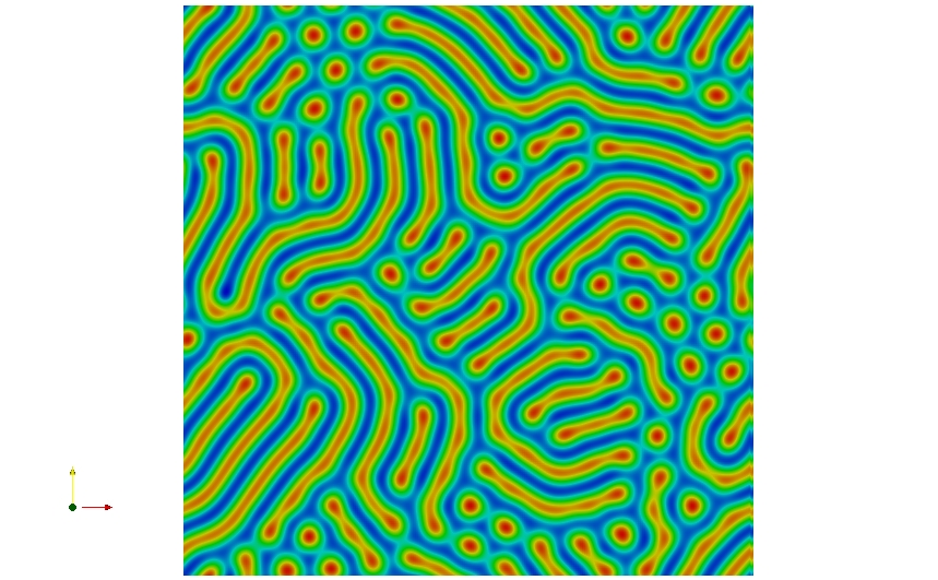
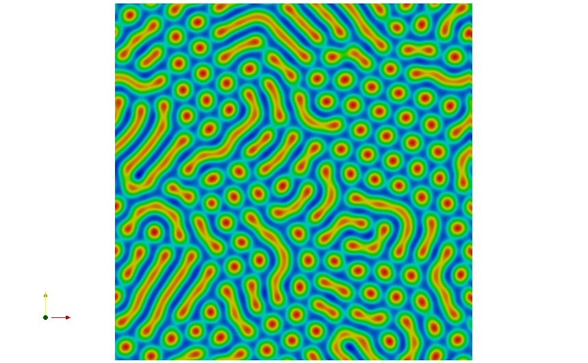
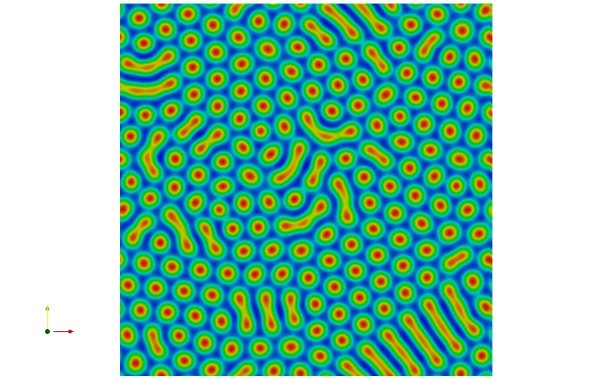
xx

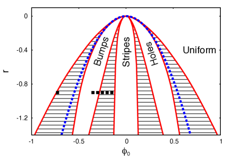
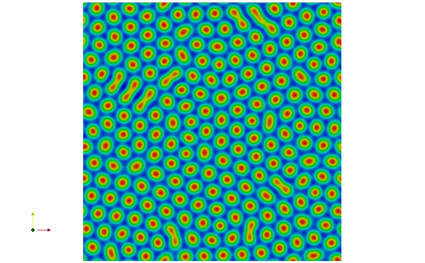
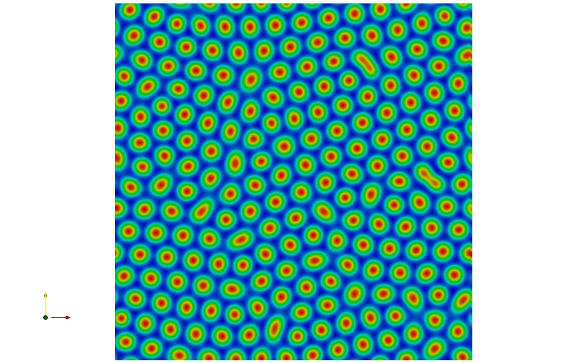
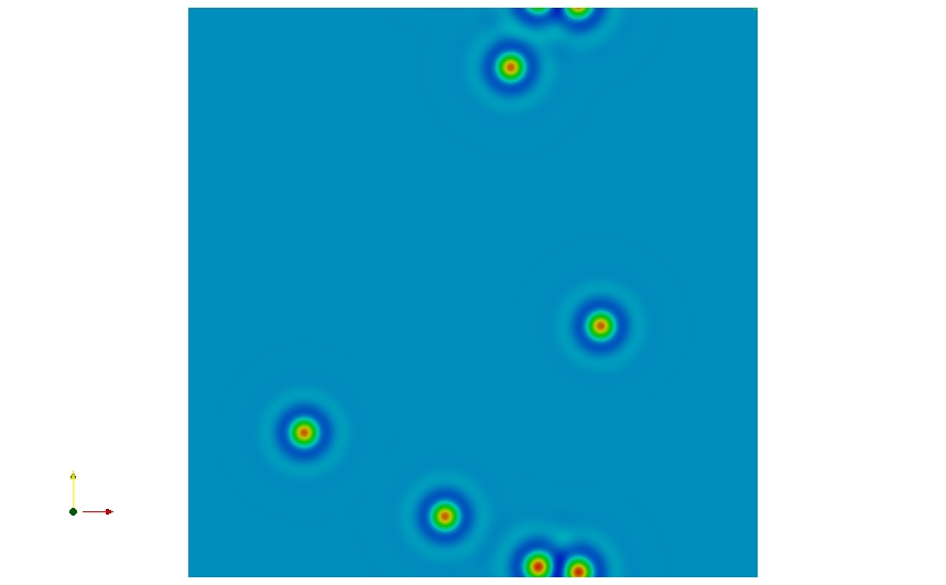
xx

Figure 9: (color online) Phase diagram for the conserved Swift-Hohenberg equation, Eq. (3), in two dimensions when $q=1$. The red solid lines show the various coexistence curves, the blue dotted line shows the limit of linear stability and the grey striped areas show phase coexistence regions. The small panels show steady solutions at $r=-0.9$ and selected mean order parameter values $\phi_{0}$ indicated by the black squares. From top to bottom left $\phi_{0}=-0.15$, $-0.2$ and $-0.25$, while from top to bottom right $\phi_{0}=-0.3$, $-0.35$ and $-0.725$. Additional solutions that detail the transition occurring between the last two panels are shown in Fig. 10. The domain size is $100\times 100$.

As in one spatial dimension, the phase diagram for two-dimensional structures helps us to identify suitable parameter values where LS are likely to occur. The phase diagram in Fig. 9, determined numerically ARTK12 , shows three distinct phases, labeled ‘bumps’, ‘stripes’ and ‘holes’. In view of the fact that $\phi(x)=\phi_{0}+\delta\phi(x)$, bumps and holes correspond to perturbations $\delta\phi(x)$ with opposite signs; both have hexagonal coordination. In addition, the phase diagram reveals four regions of thermodynamic coexistence (hatched in Fig.9), between bumps and the uniform state, between bumps and stripes, between stripes and holes, and between holes and the uniform state, respectively.

Examples of results obtained by DNS of Eq. (3) starting from random initial conditions are displayed in the side panels of Fig. 9. These six panels show results for fixed $r=-0.9$. For small values of $|\phi_{0}|$ the system forms a labyrinthine lamellar-like stripe state; the stripes pinch off locally into bumps as $|\phi_{0}|$ is increased, leading to the formation of inclusions of bumps in a background stripe state. The pinching tends to occur first at the ends of a stripe and then proceeds gradually inwards. In other cases, free ends are created by the splitting of a stripe into two in a region of high curvature. The formation of bumps tends to take place at grain boundaries, and once bump formation starts, it tends to spread outward from the initial site. For $\phi_{0}=-0.2$ the areas covered by stripes and bumps are comparable and for larger values of $|\phi_{0}|$ the bump state dominates. By $\phi_{0}=-0.3$ the stripes are almost entirely gone and the state takes the form of a crystalline solid with hexagonal coordination but having numerous defects. As $|\phi_{0}|$ increases further, vacancies appear in the solid matrix and for large enough $|\phi_{0}|$ the solid “melts” into individual bumps or smaller clusters, as further detailed in Fig. 10.

Figure 10 shows further results from a scan through decreasing values of $\phi_{0}$ at $r=-0.9$. We focus on the relatively small range $\phi_{0}=-0.45$ to $\phi_{0}=-0.675$, where localized states occur. These reveal a gradual transition from a densely packed solid-like structure to states with a progressively increasing domain area that is free of bumps, i.e., containing the homogeneous state. The bumps percolate through the domain until approximately $\phi_{0}=-0.575$. For smaller values of $\phi_{0}$ the order parameter profiles resembles a suspension of solid fragments in a liquid phase; the solid is no longer connected. As $\phi_{0}$ decreases further the characteristic size of the solid fragments decreases, as the solid fraction falls.

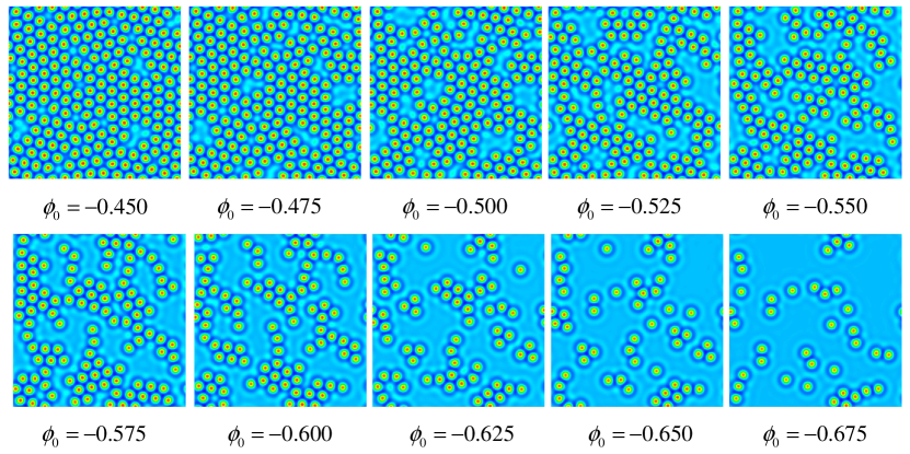
Figure 10: (color online) Steady-state solutions of the conserved Swift-Hohenberg equation, Eq. (3), in two dimensions for $r=-0.9$ and different values of $\phi_{0}$ in the range $-0.675<\phi_{0}<-0.45$, where localized states occur. The corresponding value of $\phi_{0}$ is indicated below each panel. The domain size is $100\times 100$.

IV.3 Three dimensions

In three dimensions, Eq. (3) exhibits a large number of steady state spatially periodic structures. These include those with the symmetries of the simple cubic lattice, the face-centered cubic lattice and the body-centered cubic lattice Callahan . Although we do not calculate the phase diagram for the three-dimensional (3d) system, numerical simulations in 3d reveal that a lamellar (parallel ‘sheets’) state is energetically preferred for small $\phi_{0}$. Slices through these structures resemble the stripes observed in 2d. As $|\phi_{0}|$ increases, the lamellae pinch off, much as in two dimensions, and progressively generate a 3d disordered array of bumps (Fig. 11). This solid-like state is far from being a perfect crystal, however, and with increased $|\phi_{0}|$ develops vacancies which eventually lead to its dissolution, just as in two dimensions.

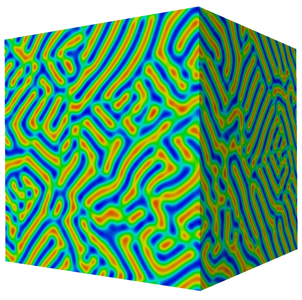
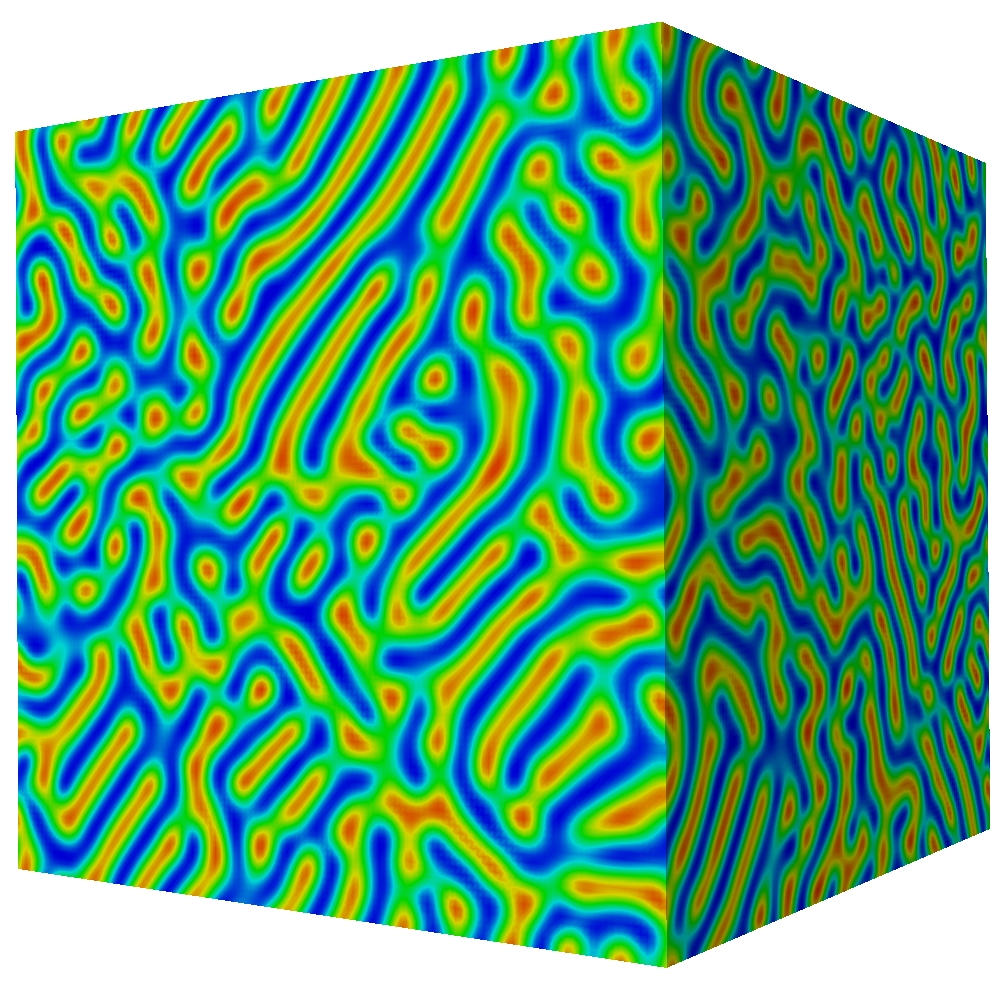
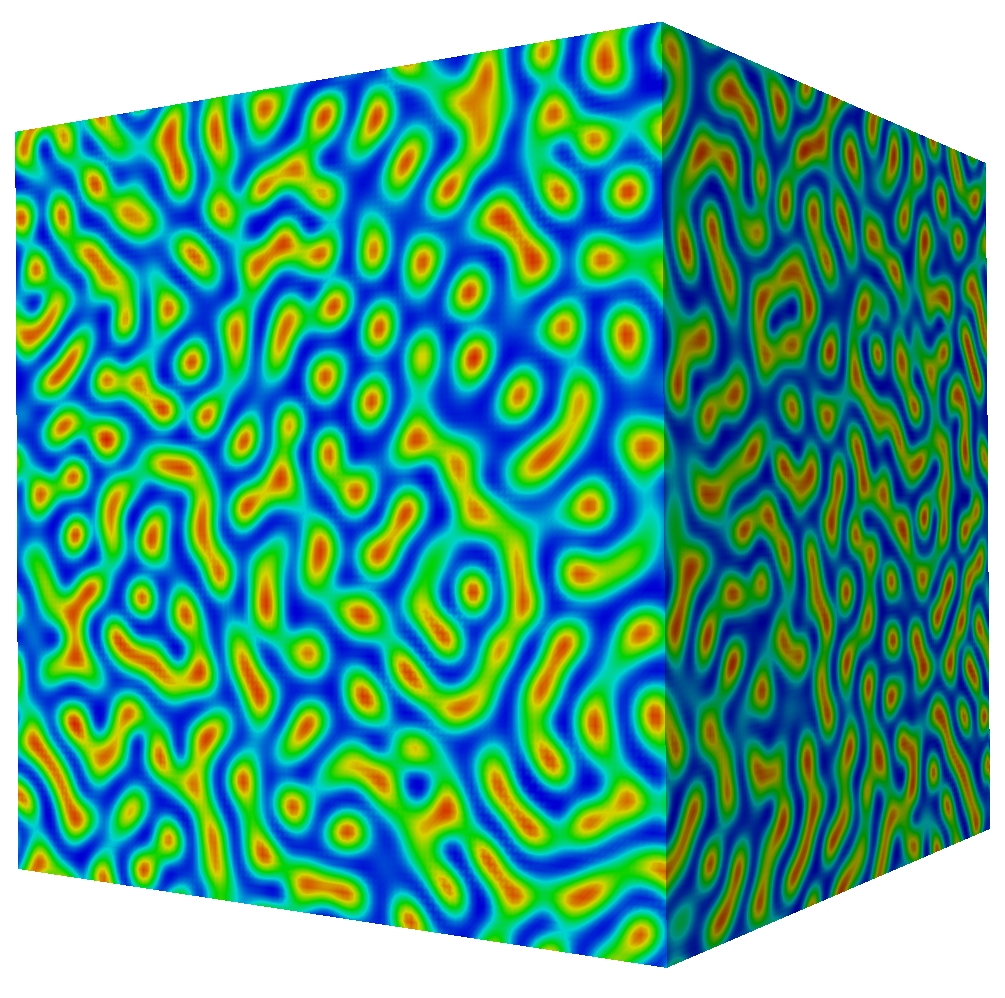
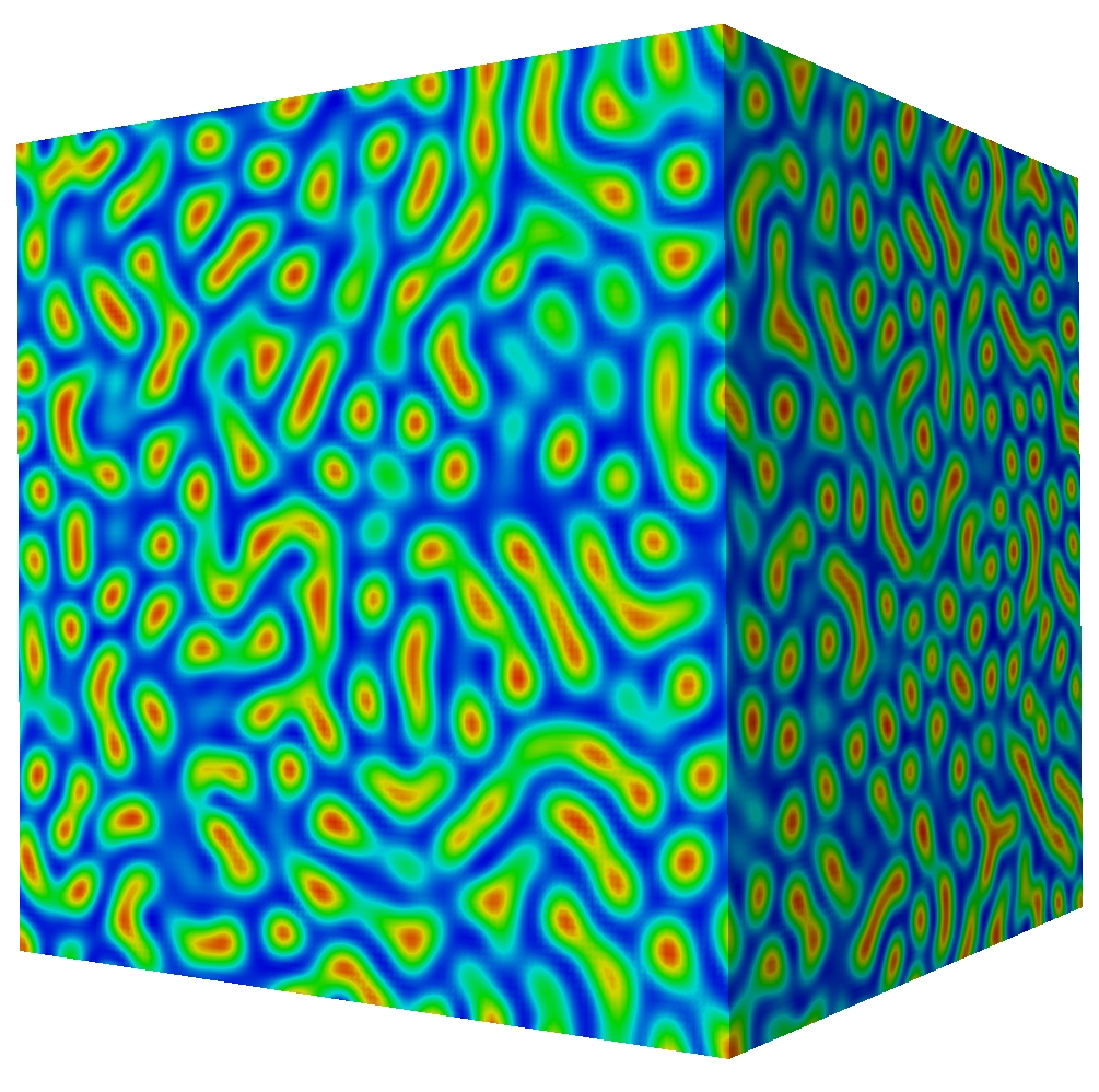
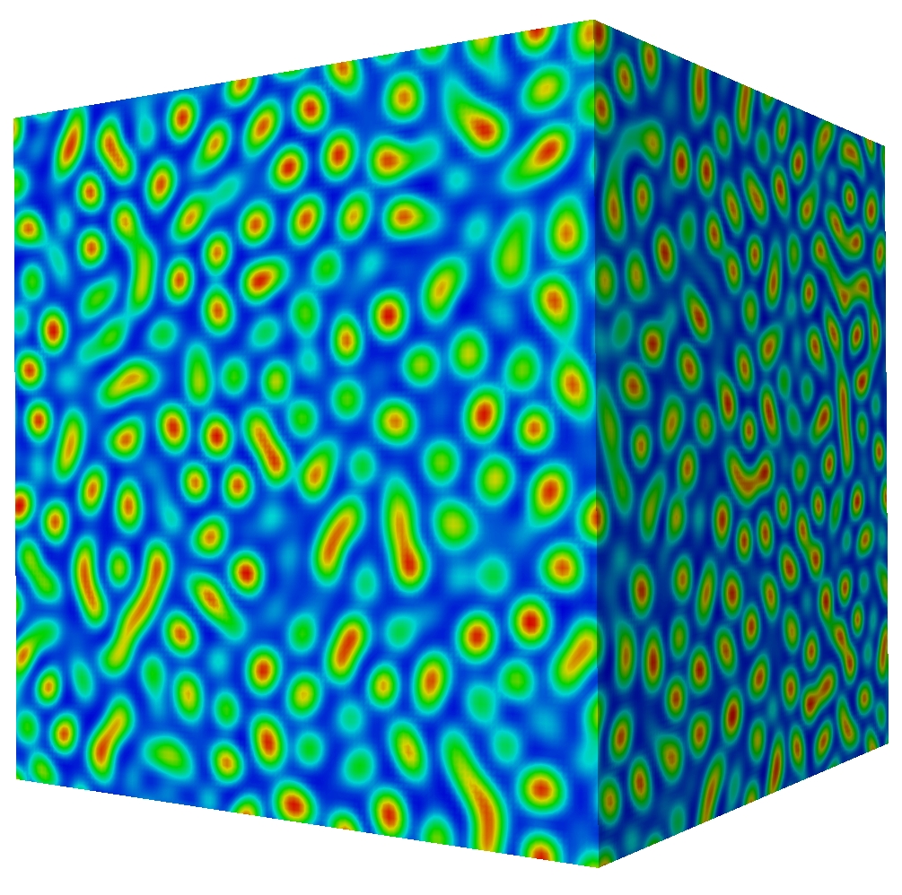
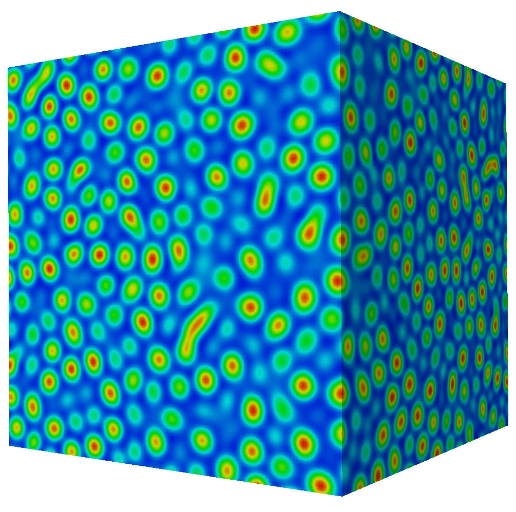
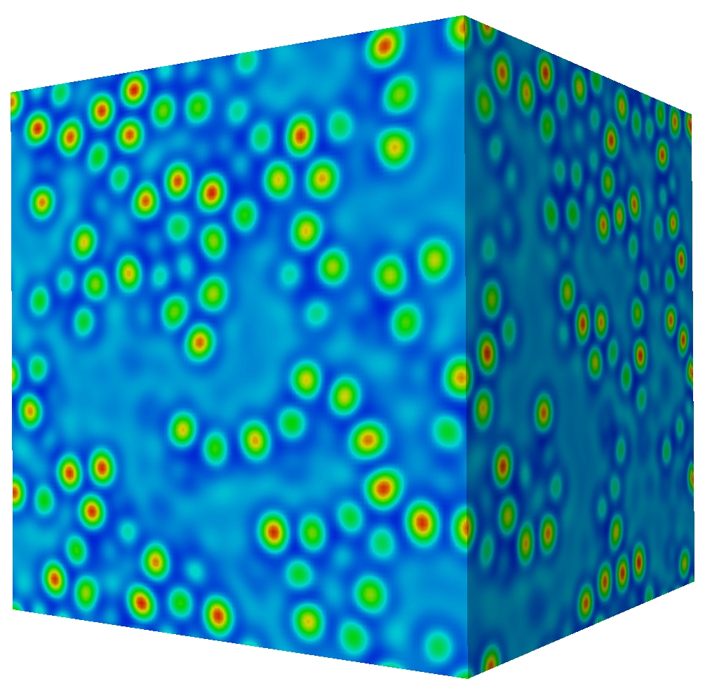
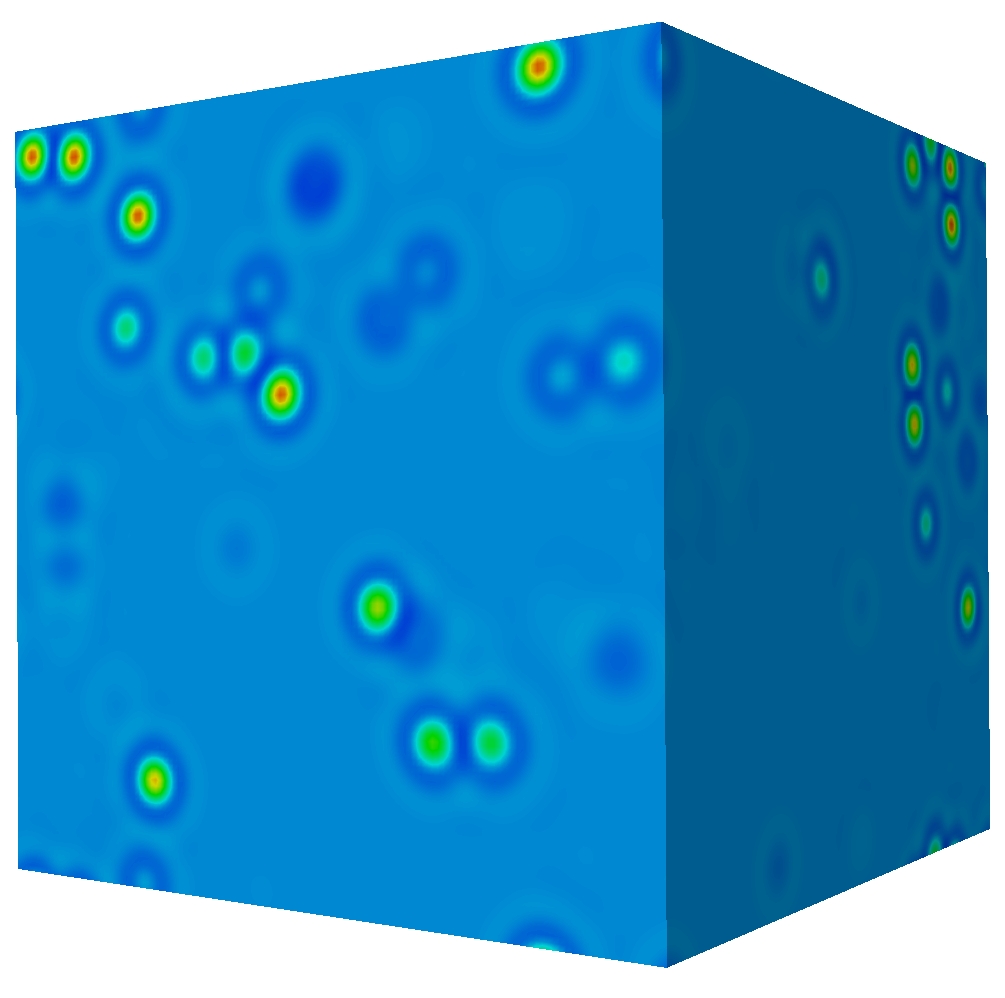
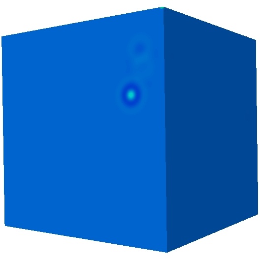
Figure 11: (color online) Steady-state localized solutions of Eq. (3) in three dimensions for $r=-0.9$ and different mean order parameter values $\phi_{0}$: from top left to bottom right $\phi_{0}=0.025,0.125,0.225,0.325,0.425,0.525,0.625,0.725$ and $0.750$. The domain size is $100\times 100\times 100$.

In Fig. 12 we superpose the 2d and 3d DNS results for $r=-0.9$ on the 1d bifurcation diagrams for $r=-0.9$ and system size $L=100$ (Fig. 2). The 2d order parameter profiles are calculated on a domain with area $L^{2}=100^{2}$ and the 3d results have a system volume $L^{3}=100^{3}$. In Fig. 12(a) we display the $L^{2}$ norm $||\delta\phi||$, in (b) the chemical potential $\mu$, in (c) the mean free energy $(F-F_{0})/L^{d}$, and in (d) the mean grand potential $\omega=F/L^{d}-\phi_{0}\mu$. In each plot the connected (violet) squares correspond to results from 2d calculations such as those displayed in Figs. 9 and 10 and the connected green triangles correspond to 3d results such as those displayed in Fig. 11. It is from examining the figures in panels (c) and (d) that one can most easily discern the reason for the main differences between the 1d results and the 2d and 3d results: we see (particularly in the 2d results) that the chemical potential $\mu$ and the pressure $p=-\omega$ have regions where these measures are roughly flat as a function of $\phi_{0}$ and regions where they increase as a function of $\phi_{0}$. We also see that these increases in some places relate to features in the 1d results but in other places they do not have any relation to what one sees from the 1d results. This is because in 2d and 3d the system displays phases that are not seen in 1d (cf. Figs. 1 and 9). To understand the origin of these roughly flat portions, we recall that in the thermodynamic limit $L\to\infty$ two states are said to be at coexistence if the ‘temperature’ $r$, the chemical potential $\mu$ and the pressure $p=-\omega$ is the same for both states. These quantities do not change in value as one takes the system across the coexistence region by increasing the average density in the system (or equivalently $\phi_{0}$). This is because the additional surface excess free energy terms (surface tension terms that are present because both coexisting phases are in the system) do not contribute in the thermodynamic limit. This is in turn a consequence of the fact that these surface terms scale as $L^{(d-1)}$, whereas the bulk volume terms scale as $L^{d}$, where $d$ is the dimensionality of the system. Thus, regions where these measures are approximately flat are in a coexistence region between two phases – this can be confirmed for the 2d results by comparing the ranges of $\phi_{0}$, where the results for $\mu$ and $\omega$ are approximately flat, with the coexistence regions in Fig. 9. The observation that the 2d curves in Fig. 12 are not completely flat indicates that the interfacial (surface tension) terms between the different phases in the LS state do contribute to the free energy, and is thus a finite size effect. Note that it might be possible to distribute the LS in such a way that they percolate throughout the whole system so that the contribution from the interfaces scales as $L^{d}$. If this is the case, the above argument does not apply.

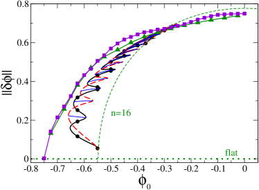
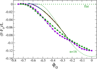
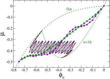
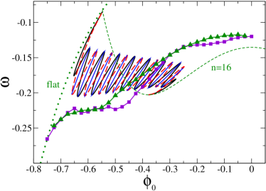
(a) (b) (c) (d)

Figure 12: (color online) Characteristics of steady-state localized solutions of the conserved Swift-Hohenberg equation for $r=-0.9$, as a function of the mean order parameter $\phi_{0}$ on fixed one, two and three-dimensional domains of size $L^{d}$, $d=1,2,3$, and $L=100$. The various solution profiles are characterized by their (a) $L^{2}$ norm $||\delta\phi||$, (b) chemical potential $\mu$, (c) mean free energy $(F-F_{0})/L^{d}$, and (d) mean grand potential $\omega=F/L^{d}-\phi_{0}\mu$. The connected (violet) square and (green) triangle symbols correspond to 2d calculations (for sample profiles see Figs. 9 and 10) and 3d calculations (for sample profiles see Fig. 11). For comparison we also show the 1d results from Fig. 2 for the periodic (i.e., stripe) state with $n=16$ bumps, green dashed) and the various 1d localized states. The thick green dotted line corresponds to the homogeneous solution $\phi(\mathbf{x})=\phi_{0}$.

V Discussion and conclusions

The conserved Swift-Hohenberg equation is perhaps the simplest example of a pattern-forming system with a conserved quantity. Models of this type arise when modelling a number of different systems, with the PFC model being one particular example. Other examples include binary fluid convection between thermally insulating boundaries K:89 , where this equation was first derived, convection in an imposed magnetic field (where the conserved quantity is the magnetic flux CM01 ; LBK11 ) and two-dimensional convection in a rotating layer with stress-free boundaries (where the conserved quantity is the zonal velocity CM01 ; BBKK12 ). Models of a vibrating layer of granular material are also of this type (here the conserved quantity is the total mass DL10 ). It is perhaps remarkable that all these distinct systems behave very similarly. In particular, they all share the following features: (i) strongly subcritical bifurcations forming localized structures so that the resulting LS are present outside of the bistability region between the homogeneous and periodic states; (ii) presence of LS even when the periodic branch is supercritical; (iii) organization of LS into slanted snaking; and (iv) the transition from slanted snaking to smooth snaking whereby the LS grow smoothly without specific bump-forming events (referred to as ‘nucleation’ events in the pattern formation literature .) These properties of the system can all be traced to the fact that the conserved quantity is necessarily redistributed when an instability takes place or a localized structure forms. This fact makes it harder for additional LS to form and as a result the system has to be driven harder for this to occur, leading to slanted snaking. Bistability is no longer required since the localized structures are no longer viewed as inclusions of a periodic state within a homogeneous background or vice versa. These considerations also explain why the bifurcation diagrams in these systems are sensitive to the domain size, and it may be instructive, although difficult, to repeat some of our calculations for larger domain sizes.

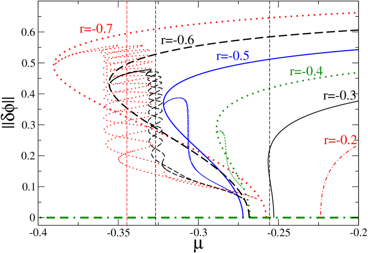
Figure 13: (color online) The $L^{2}$ norm $||\delta\phi||$ for the homogeneous, periodic and localized steady state solutions of the conserved Swift-Hohenberg equation (3) as a function of the chemical potential $\mu$, for a fixed domain size of $L=100$ and various $r$. The horizontal thick dot-dashed green line corresponds to the homogeneous solution $\phi(x)=\phi_{0}$. Periodic solutions with $n=16$ peaks are labeled by the corresponding $r$ values, whereas the branches that bifurcate from the periodic solution branches represent the two types of symmetric localized states (LS_odd and LS_even): $r=-0.7$ (dotted red lines), $r=-0.6$ (dashed black lines), $r=-0.5$ (solid blue lines), $r=-0.4$ (dotted green lines), $r=-0.3$ (solid black line) and $r=-0.2$ (dashed red line). The dashed vertical lines indicate the corresponding coexistence chemical potential values for $r=-0.7$, $-0.6$ and $-0.3$, respectively.

Of particular significance is the observation that the slanted snaking found when the LS norm $||\delta\phi||$ is plotted as a function of the mean order parameter $\phi_{0}$ for fixed $r$ (Figs. 2 and 4(a,b)) is ‘straightened’ out when the same solution branches are displayed as a function of $\mu$ (see Fig. 13). The snaking is then vertically aligned and centred around the coexistence chemical potential values (referred to as Maxwell points in Ref. BuKn06 ) as known from the non-conserved Swift-Hohenberg equation BuKn06 . In this representation the periodic states typically bifurcate subcritically from the homogeneous state (Fig. 13), in contrast to the supercritical transitions found when $\phi_{0}$ is used as the bifurcation parameter (Figs. 2 and 4). It is also worth noting that the thermodynamic tricritical point at $(\phi_{0b},r_{b}^{\mathrm{max}})=(\pm\sqrt{3/38},-9/38)$ discussed in Sec. II.2 (see also the last paragraph of the Appendix) corresponds to the transition from a subcritical to a supercritical primary bifurcation in the representation of Fig. 13, i.e., when $\mu$ is used as the bifurcation parameter. This transition takes place between the solid black line for $r=-0.3$ and the dashed red line for $r=-0.2$ in Fig. 13 and implies that the linear stability properties of identical periodic solutions differ, depending on whether the permitted perturbations preserve $\mu$ (and hence permit $\phi_{0}$ to vary) or vice versa, and this is so for the localized states as well. In particular, when $\mu$ is used as the control parameter, the differences identified in Sec. III.2 between cases (i)-(iv) where the LS branches do not snake, and cases (v)-(vi) where they do snake disappear. In Fig. 13 snaking over $\mu$ is clearly visible for $r=-0.7$, $-0.6$ and $-0.5$. There is no snaking for $r=-0.4$, most likely due to finite size effects, or for larger $r$.

The thermodynamic reason that the snaking becomes straightened when displayed as a function of the chemical potential $\mu$ is related to the issues discussed at the end of Sec. IV. For a system with $(\phi_{0},r)$ chosen so that it is in the coexistence region (e.g., between the homogeneous and the bump states) and size $L$ large enough to be considered to be in the thermodynamic limit $L\to\infty$, the chemical potential does not vary when $\phi_{0}$ is changed and neither does the grand potential $\omega=-p$. This is because the free energy contribution from interfaces between the coexisting phases (the interfacial tension) scales with the system size $\sim L^{(d-1)}$, and hence is negligible compared to the bulk contributions which scale $\sim L^{d}$. As $\phi_{0}$ is varied so as to traverse the coexistence region, new bumps are added or removed from the bump state (LS). For a (thermodynamically) large system, the resulting changes in the free energy are negligible, although this is no longer true of a finite size system. Furthermore, the interfacial free energy contribution between the two phases varies depending on the size of the bumps right at the interface and the size of these bumps depends on the value of $\phi_{0}$. The difference between the maximal interfacial energy and the minimal value determines the width of the snake. All of these contributions have leading order terms that scale $\sim L^{-1}$. In a related situation, the variation in the chemical potential as the density is varied in a finite-size system containing a fluid exhibiting gas-liquid coexistence is discussed in Refs. MSE06 ; SVB09 ; BBVT12 . It is instructive to compare, for example, Fig. 3 in Ref. BBVT12 and Fig. 12(c) of the present paper.

We mention that the steady states of the nonconserved Swift-Hohenberg equation studied, e.g., in Refs. BuKn06 ; BBKM08 , correspond to solutions of Eq. (5) with the nonlinearity $g_{23}$ but $\mu=0$ (see Sec. II.1). These always show vertically aligned snaking when the LS norm $||\delta\phi||$ is plotted as a function of $r$ (adapting $\phi_{0}$). However, when $\mu=0$ no localized states are present with the pure cubic nonlinearity employed in Eq. (5). To find such states $\mu$ must be fixed at a value sufficiently far from zero; the resulting LS then exhibit vertically aligned snaking when plotted as a function of $r$ BuKn06 .

The domain size we have used, $L=100$, is moderately large. It contains of the order of 16 wavelengths of the primary structure-forming instability. Because the equation is simpler than the hydrodynamic equations for which similar behavior was observed, the results we have been able to obtain are substantially more complete, even in one dimension, than was possible elsewhere. In particular, we have been able to compute the rungs of asymmetric LS and to study their behavior as the system transitions from slanted snaking to smooth snaking as $r$ increases towards zero. The extension of our results to two and three spatial dimensions is necessarily incomplete, although the transition to clusters of bumps followed by isolated bumps as the total “mass” decreases is not surprising. However, the transition from a connected structure to a disconnected one (the “percolation” threshold) in two and three dimensions deserves a much more detailed study than we have been able to provide.

In this connection we mention two experimental systems exhibiting a transition from a solid-like phase to a gas-like phase of individual spots. This is the gaseous discharge system studied by H.-G. Purwins and colleagues astrov01 ; PBA10 and the liquid crystal light valve experiment of S. Residori and colleagues BCR09 . In both these systems a crystal-like structure of spots with hexagonal coordination was observed to melt into a ‘gas’ of individual spots as a parameter was varied. This two-dimensional process leads to states resembling those found here in Figs. 9 and 10 although the stripe-like structures were typically absent. In these two systems the spots in the ‘gas-phase’ are mobile unlike in the cSH equation indicating absence of variational structure. However, both systems are globally coupled, by the imposed potential difference in the discharge system and the feedback loop in the liquid crystal light valve experiment, raising the possibility that the global coupling in these systems plays a similar role to the role played by the conserved order parameter in the cSH equation.

We should also mention that some of the localized states observed in Figs. 10 and 11 raise some concern about the validity of the PFC as a model for solidification and freezing – we refer in particular to the order parameter profiles displayed at the bottom right of these figures. These show that in both 2d and 3d the PFC predicts the existence of steady states with isolated single bumps. Recall that in the standard interpretation of the PFC, the bumps correspond to frozen particles whilst the homogeneous state corresponds to the uniform liquid state. Such profiles could perhaps be a signature of the dynamical heterogeneity that is a feature of glassy systems, but there are problems with this interpretation – the glass transition is a collective phenomenon – single particles do not freeze on their own whilst the remainder of the particles around them remain fluid! We refer readers interested in the issue of the precise interpretation of the order parameter in the PFC to the discussion in the final section of Ref. RATK12 . We should also point out that although these structures correspond to local minima of the free energy (i.e., they are stable) they do not correspond to the global minimum. These states occur for state points where the global free energy minimum corresponds to the uniform homogeneous state.

All the results presented here have been obtained for the generic conserved Swift-Hohenberg equation, Eq. (1), with the energy functional in Eq. (2). We believe that our main results provide a qualitative description of a number of related models in material science that are of a similar structure and describe systems that may show transitions between homogeneous and patterned states characterized by a finite structure length. In particular, we refer to systems that can be described by conserved gradient dynamics based on an underlying energy functional that features a local double-well contribution, a destabilizing squared gradient term and a stabilizing squared Laplacian term. The latter two terms may themselves result from a gradient expansion of an integral describing nonlocal interactions such as that required to reduce DDFT models to the simpler PFC model vBVL09 ; ARTK12 .

Other systems, where the present results may shed some light, include diblock copolymers and epitaxial layers. The time evolution equation for diblock copolymers OoSh87 ; Paqu91 ; TeNi02 ; Glas10 ; Glas12 is of fourth order like the nonconserved SH equation but contains a global coupling term that is related to mass conservation. The equation emerges from a nonlocal term in the energy functional Leib80 ; OhKa86 . The global coupling results in an evolution towards a state with a given mean value for the density order parameter $\phi_{0}$ if the initial value is different from $\phi_{0}$ or in a conservation of mass as the system evolves if the initial value coincides with the imposed $\phi_{0}$. Although this differs from the formulation using a conserved Swift-Hohenberg equation, the steady versions of the diblock-copolymer equation and of the conserved Swift-Hohenberg equation are rather similar: they only differ in the position of the nonlinearity. Up to now no systematic study of localized states exists for the diblock-copolymer equation, although Ref. Glas12 discusses their existence and gives some numerical examples for a profile with a single bump in rather small systems (see their Fig. 5). Since in the diblock-copolymer system the order parameter is a conserved quantity, we would expect the snaking of localized states for fixed $\phi_{0}$ to be slanted similar to our Fig. 2, instead of being vertical, corresponding to a standard snake, where all the saddle-node bifurcations are vertically aligned, as sketched in Fig. 6 of Glas12 .

Finally, we briefly mention a group of model equations that are derived to describe the evolution of the surface profile of epitaxially strained solid films including, e.g., the self-organization of quantum dots GDV03 . The various evolution equations that have been employed account for the elasticity (linear and nonlinear isotropic elasticity, as well as misfit strain) of the epitaxial layer and the (isotropic or anisotropic) wetting interaction between the surface layer and the solid beneath. The evolution equations we wish to highlight are of sixth order SDV93 ; Savi03 ; GLSD04 ; Thie10 much like the conserved Swift-Hohenberg equation investigated here. Other models, however, are of fourth order only XiE02 ; SRF03 or contain fully nonlocal terms (resulting in integro-differential equations) XiE04 ; LGDV07 . However, even the sixth order models often contain additional nonlinear terms in the derivatives (see, for instance, Eq. (5) of Ref. GDV03 ). Localized state solutions of these equations have to our knowledge not yet been studied systematically, although some have been obtained numerically (Fig. 5 of GDV03 ). Future research should investigate how the characteristics of the localized states analysed here for the conserved Swift-Hohenberg equation differ from those in specific applied systems such as diblock copolymers or epitaxial layers.

Appendix

In this Appendix we determine the direction of branching of the localized states when they bifurcate from the branch of periodic states. When the domain is large this bifurcation occurs when the amplitude of the periodic states is small and hence is accessible to weakly nonlinear theory.

We begin with Eq. (4) which may be written

$$\phi_{t}=\alpha\partial_{x}^{2}[(r+q^{4})\phi+\phi^{3}+2q^{2}\partial_{x}^{2}\phi+\partial_{x}^{4}\phi].$$ (11)

This equation has the homogeneous solution $\phi=\phi_{0}$. We let $\phi=\phi_{0}+\psi$, obtaining

$$\psi_{t}=\alpha\partial_{x}^{2}[(r+q^{4}+3\phi_{0}^{2})\psi+3\phi_{0}\psi^{2}+\psi^{3}+2q^{2}\partial_{x}^{2}\psi+\partial_{x}^{4}\psi].$$ (12)

Linearizing and looking for solutions of the form $\psi\propto\exp(\beta t+ikx)$ we obtain the dispersion relation

$$\beta=-\alpha k^{2}[r+(q^{2}-k^{2})^{2}+3\phi_{0}^{2}]$$ (13)

The condition $\beta=0$ gives the critical wavenumbers

$$k_{c}^{2}=q^{2}\pm\sqrt{-r-3\phi_{0}^{2}}$$ (14)

Thus when $r=r_{c}\equiv-3\phi_{0}^{2}$ the neutral curve has maxima at both $k=0$ and $k_{c}=q$. When $r=-3\phi_{0}^{2}-\epsilon^{2}\nu$, where $\nu={\cal O}(1)$ and $\epsilon$ is a small parameter that defines how far $r$ is from $r_{c}$, then a band of wavenumbers near $k=q$ grows slowly with growth rate $\beta={\cal O}(\epsilon^{2})$, while wavenumbers near $k=0$ decay at the same rate. There is therefore time for these two disparate wavenumbers to interact and it is this interaction that determines the direction of branching.

These considerations suggest that we perform a two-scale analysis with a short scale $x={\cal O}(q^{-1})$ and a long scale $X=\epsilon x$, so that $\partial_{x}\rightarrow\partial_{x}+\epsilon\partial_{X}$ etc. We also write

$$\psi=\epsilon A(X,t)e^{iqx}+\epsilon^{2}B(X,t)+\epsilon^{2}C(X,t)e^{2iqx}+{\rm c.c.}+{\cal O}(\epsilon^{3}),$$ (15)

where the amplitudes $A$ and $C$ are complex and $B$ is real. Substituting, we obtain

$$A_{t}=-\epsilon^{2}\alpha q^{2}(-\nu A-4q^{2}A_{XX}+6\phi_{0}AB+6\phi_{0}CA^{*}+3|A|^{2}A)+{\cal O}(\epsilon^{3}),$$ (16)

$$B_{t}=\epsilon^{2}\alpha(q^{4}B_{XX}+6\phi_{0}|A|^{2}_{XX})+{\cal O}(\epsilon^{3}),$$ (17)

and

$$C_{t}=-4\alpha q^{2}(9q^{4}C+3\phi_{0}A^{2})+{\cal O}(\epsilon).$$ (18)

The last equation implies that the mode $C$ decays on an ${\cal O}(1)$ time scale to its asymptotic value, $C=-\phi_{0}A^{2}/3q^{4}+{\cal O}(\epsilon)$. The resulting equations may be written in the form

$$A_{t}=\nu A+4A_{XX}-\xi A\theta_{X}-3\biggl{(}1-\frac{\xi^{2}}{54}\biggr{)}|A|^{2}A+{\cal O}(\epsilon),$$ (19)

$$\theta_{t}=\theta_{XX}+\xi|A|^{2}_{X}+{\cal O}(\epsilon)$$ (20)

using the substitution $B=\theta_{X}$, and integrating Eq. (17) once to obtain an equation for $\theta$. In writing these equations we have absorbed $q$ into the length scale $X$ and $\epsilon^{2}\alpha q^{2}$ into the time scale $t$, and introduced the parameter $\xi\equiv 6\phi_{0}/q^{2}<0$. The resulting equation are equivalent to the equations studied by Matthews and Cox MaCo00 .

Equations (19)–(20) provide a complete description of the small amplitude behavior of Eq. (4). The equations inherit a gradient structure from Eq. (4),

$$A_{t}=-\frac{\delta F}{\delta A^{*}},\qquad\theta_{t}=-\frac{\delta F}{\delta\theta},$$ (21)

where

$$F[A,A^{*},\theta]=\int_{D}\biggl{\{}-\nu|A|^{2}+4|A_{X}|^{2}+\frac{1}{2}\theta_{X}^{2}+\xi|A|^{2}\theta_{X}+\frac{3}{2}\biggl{(}1-\frac{\xi^{2}}{54}\biggr{)}|A|^{4}\biggr{\}}\,dX.$$ (22)

We may write this energy in the form

$$F[A,A^{*},\theta]=\int_{D}\biggl{\{}-\nu|A|^{2}+4|A_{X}|^{2}+\frac{1}{2}\bigg{[}(\theta_{X}+\xi|A|^{2})^{2}+3\biggl{(}1-\frac{19\xi^{2}}{54}\biggr{)}|A|^{4}\biggr{]}\biggr{\}}\,dX,$$ (23)

implying that the free energy $F[A,A^{*},\theta]$ is not bounded from below once $\xi^{2}>54/19$ (equivalently $\phi_{0}^{2}>3q^{4}/38$). This is a reflection of the presence of subcritical branches. Indeed, the steady states of Eqs. (19)–(20) correspond to critical points of this energy and satisfy the nonlocal equation

$$4A_{XX}+(\nu-\langle|A|^{2}\rangle)A-3\biggl{(}1-\frac{19\xi^{2}}{54}\biggr{)}|A|^{2}A=0,$$ (24)

where $\langle(\cdots)\rangle\equiv L^{-1}\int_{0}^{L}(\cdots)\,dx$ and $L$ is the domain length. This equation demonstrates (i) that the primary bifurcation is subcritical when $\xi^{2}>54/19$ in agreement with Eq. (23), and (ii) that as $|A|$ increases the value of $\nu$ has to be raised in order to maintain the same value of the effective bifurcation parameter ${\nu}_{\rm eff}\equiv\nu-\langle|A|^{2}\rangle$. This is the basic reason behind the slanted structure in Fig. 2(a). Equations of this type arise in numerous applications hall ; Elmer88a ; Elmer88b ; BBKK12 and their properties have been studied in several papers Elmer88a ; norbury02 ; vega05 ; norbury07 . We mention, in particular, that unmodulated wavetrains bifurcate supercritically when $\xi^{2}<54$, a condition that differs from the corresponding condition $\xi^{2}<54/19$ for spatially modulated wavetrains.

Equations (19)–(20) possess the solution $(A,\theta)=(A_{0},0)$, where $|A_{0}|^{2}=\nu/[3(1-\xi^{2}/54)]$, corresponding to a spatially uniform wavetrain. This state bifurcates in the positive $\nu$ direction wherever $\xi^{2}<54$, or equivalently $\phi_{0}^{2}<3q^{4}/2$. In the following we are interested in the modulational instability of this state. We suppose that this instability takes place at $\nu=\nu_{c}$ and write $\nu=\nu_{c}+\delta^{2}{\tilde{\nu}}$, where $\delta\ll\epsilon$ is a new small parameter and ${\tilde{\nu}}={\cal O}(1)$. In addition, we write $A=A_{0}(1+{\tilde{A}})$, $\theta_{X}={\tilde{V}}$. Since the imaginary part of ${\tilde{A}}$ decays to zero we take ${\tilde{A}}$ to be real and write

$${\tilde{A}}=\delta{\tilde{A}}_{1}+\delta^{2}{\tilde{A}}_{2}+\delta^{3}{\tilde{A}}_{3}+\dots,\quad{\tilde{V}}=\delta{\tilde{V}}_{1}+\delta^{2}{\tilde{V}}_{2}+\delta^{3}{\tilde{V}}_{3}+\dots.$$ (25)

Finally, since the localized states created at $\nu_{c}$ are stationary, we set the time derivatives to zero and integrate Eq. (20) once obtaining

$${\tilde{V}}+\xi|A|^{2}+C(\delta)=0,$$ (26)

where $C=C_{0}+\delta C_{1}+\delta^{2}C_{2}+\delta^{3}C_{3}+\dots$ and the $C_{j}$ are determined by the requirement that the average of $V$ over the domain vanishes.

Substitution of the above expressions yields a sequence of ordinary differential equations which we solve subject to periodic boundary conditions. At ${\cal O}(1)$ we obtain $C_{0}=-\xi|A_{c}|^{2}$, where $A_{c}$ denotes the value of $A_{0}$ at $\nu=\nu_{c}$. At ${\cal O}(\delta)$ we obtain the linear problem

$$-2\nu_{c}{\tilde{A}}_{1}+4{\tilde{A}}_{1XX}-\xi{\tilde{V}}_{1}=0,\qquad{\tilde{V}}_{1}+2\xi|A_{c}|^{2}{\tilde{A}}_{1}=0,\qquad C_{1}=0,$$ (27)

and conclude that ${\tilde{A}}_{1}=A_{11}\cos\ell X$, ${\tilde{V}}_{1}=V_{11}\cos\ell X$, provided that $\nu_{c}=-2\ell^{2}[(1-\xi^{2}/54)/(1-19\xi^{2}/54)]$. Note that this quantity is positive when $54>\xi^{2}>54/19$ (equivalently $3q^{4}/2>\phi_{0}^{2}>3q^{4}/38$) and that it vanishes in the limit $\ell\rightarrow 0$, i.e., for infinite modulation length scale.

At ${\cal O}(\delta^{2})$ we obtain

$$-2\nu_{c}{\tilde{A}}_{2}+4{\tilde{A}}_{2XX}-\xi{\tilde{V}}_{2}=\xi{\tilde{A}}_{1}{\tilde{V}}_{1}+3\nu_{c}{\tilde{A}}_{1}^{2},\qquad{\tilde{V}}_{2}+\xi|A_{c}|^{2}(2{\tilde{A}}_{2}+{\tilde{A}}_{1}^{2})+C_{2}=0.$$ (28)

Thus ${\tilde{A}}_{2}=A_{20}+A_{22}\cos 2\ell X$, ${\tilde{V}}_{2}=V_{22}\cos 2\ell X$, where

$$A_{20}=-\frac{3}{4}\biggl{[}\frac{1-(13\xi^{2}/54)}{1-(\xi^{2}/54)}\biggl{]}A_{11}^{2},\qquad A_{22}=\frac{1}{4}A_{11}^{2},\qquad V_{22}=-\xi|A_{c}|^{2}A_{11}^{2},$$ (29)

together with

$$C_{2}=-\frac{1}{2}\xi|A_{c}|^{2}A_{11}^{2}-2\xi|A_{c}|^{2}A_{20}.$$ (30)

Finally, at ${\cal O}(\delta^{3})$ we obtain

$$-2\nu_{c}{\tilde{A}}_{3}+4{\tilde{A}}_{3XX}-\xi{\tilde{V}}_{3}=2{\tilde{\nu}}{\tilde{A}}_{1}+\xi({\tilde{A}}_{1}{\tilde{V}}_{2}+{\tilde{A}}_{2}{\tilde{V}}_{1})+\nu_{c}(6{\tilde{A}}_{1}{\tilde{A}}_{2}+{\tilde{A}}_{1}^{3}),$$ (31)

and

$${\tilde{V}}_{3}+\xi|A_{c}|^{2}(2{\tilde{A}}_{3}+2{\tilde{A}}_{1}{\tilde{A}}_{2})+C_{3}=-\frac{2\xi}{3(1-(\xi^{2}/54))}{\tilde{\nu}}{\tilde{A}}_{1}.$$ (32)

The direction of branching of solutions with ${\tilde{A}}\neq 0$ follows from the solvability condition for ${\tilde{A}}_{3}$, i.e., the requirement that the inhomogeneous terms contain no terms proportional to $\cos\ell X$. We obtain

$${\tilde{\nu}}+3\ell^{2}{\tilde{A}}_{11}^{2}\biggl{[}\frac{1-(13\xi^{2}/54)}{1-(19\xi^{2}/54)}\biggr{]}=0.$$ (33)

It follows that the localized states bifurcate in the positive $\nu$ direction (lower temperature) when $54/19<\xi^{2}<54/13$ and in the negative $\nu$ direction when $54/13<\xi^{2}<54$. The former requirement is equivalent to $3q^{4}/38<\phi_{0}^{2}<3q^{4}/26$, the latter to $3q^{4}/26<\phi_{0}^{2}<3q^{4}/2$. These results agree with the corresponding results for an equation similar to Eq. (24) obtained by Elmer Elmer88a (see also MaCo00 ; BBKK12 ).

In the above calculation we have fixed the parameter $\xi$ (equivalently $\phi_{0}$) and treated $r$ (equivalently $\nu$) as the bifurcation parameter. However, we can equally well do the opposite. Since the calculation is only valid in the neighborhood of the primary bifurcation at $r=-3\phi_{0}^{2}$, i.e., in the neighborhood of $\xi=-\sqrt{-12r}/q^{2}$, the destabilizing perturbation analogous to ${\tilde{\nu}}>0$ is now replaced by ${\tilde{\xi}}>0$ (cf. Fig. 1), implying that the direction of branching of localized states changes from subcritical to supercritical as $\xi^{2}$ decreases through $\xi^{2}=54/13$ (equivalently $\phi_{0}^{2}$ decreases through $\phi_{0}^{2}=3q^{4}/26$ or $r$ increases through $r=-9q^{4}/26\approx-0.35q^{4}$), in good agreement with the numerically obtained value $r\approx-0.41$ (for $q=1$) that is indicated in Fig. 7 by the horizontal line separating regions (iii) and (iv).

We next consider the corresponding results in the case when the chemical potential $\mu$ is fixed. In this case the constants $C_{j}$ vanish, and the ${\cal O}(\delta^{2})$ problem therefore has solutions of the form ${\tilde{A}}_{2}=A_{20}+A_{22}\cos 2\ell X$, ${\tilde{V}}_{2}=V_{20}+V_{22}\cos 2\ell X$, where

$$A_{20}=-\frac{3}{4}A_{11}^{2},\qquad V_{20}=\xi|A_{c}|^{2}A_{11}^{2},\qquad A_{22}=\frac{1}{4}A_{11}^{2},\qquad V_{22}=-\xi|A_{c}|^{2}A_{11}^{2}.$$ (34)

The nonzero $V_{20}$ contributes additional terms to the solvability condition at ${\cal O}(\delta^{3})$. The result corresponding to (33) is

$${\tilde{\nu}}+3\ell^{2}{\tilde{A}}_{11}^{2}\biggl{[}\frac{1-(\xi^{2}/54)}{1-(19\xi^{2}/54)}\biggr{]}=0.$$ (35)

This implies that the secondary LS branches are subcritical whenever the periodic branch is supercritical ($\xi^{2}<54$) and the secondary bifurcation is present ($\xi^{2}>54/19$). These results are consistent with Fig. 13 and moreover predict that the LS states are absent for $\xi^{2}<54/19$, i.e., for $\phi_{0}>-\sqrt{3/38}q^{2}$ or $r>-9q^{4}/38$ (cf. Fig. 13). This point is, of course, the thermodynamic tricritical point discussed in Sec. II.2.

Acknowledgement. The authors wish to thank the EU for financial support under grant MRTN-CT-2004-005728 (MULTIFLOW) and the National Science Foundation for support under grant DMS-1211953.

References

- (1) P. Coullet, C. Riera, and C. Tresser, “Stable static localized structures in one dimension,” Phys. Rev. Lett. 84, 3069–3072 (2000).
- (2) U. Bortolozzo, M. G. Clerc, and S. Residori, “Solitary localized structures in a liquid crystal,” New. J. Phys. 11, 093037 (2009).
- (3) R. Richter and I. V. Barashenkov, “Two-dimensional solitons on the surface of magnetic fluids,” Phys. Rev. Lett. 94, 184503 (2005).
- (4) G. W. Hunt, M. A. Peletier, A. R. Champneys, P. D. Woods, M. A. Wadee, C. J. Budd, and G. J. Lord, “Cellular buckling in long structures,” Nonlinear Dynamics 21, 3–29 (2000).
- (5) O. Batiste, E. Knobloch, A. Alonso, and I. Mercader, “Spatially localized binary-fluid convection,” J. Fluid Mech. 560, 149–158 (2006).
- (6) A. Bergeon and E. Knobloch, “Spatially localized states in natural doubly diffusive convection,” Phys. Fluids 20, 034102 (2008).
- (7) S. Blanchflower, “Magnetohydrodynamic convectons,” Phys. Lett. A 261, 74–81 (1999).
- (8) T. M. Schneider, J. F. Gibson, and J. Burke, “Snakes and ladders: localized solutions of plane Couette flow,” Phys. Rev. Lett. 104, 104501 (2010).
- (9) O. Lioubashevski, H. Arbell, and J. Fineberg, “Dissipative solitary waves in driven surface waves,” Phys. Rev. Lett. 76, 3959–3962 (1996).
- (10) J. Rajchenbach, A. Leroux, and D. Clamond, “New standing solitary waves in water,” Phys. Rev. Lett. 107, 024502 (2011).
- (11) P. B. Umbanhowar, F. Melo, and H. L. Swinney, “Localized excitations in a vertically vibrated granular layer,” Nature 382, 793–796 (1996).
- (12) T. Ackemann, W. J. Firth, and G.-L. Oppo, “Fundamentals and applications of spatial dissipative solitons in photonic devices,” in P. R. Berman, E. Arimondo, and C.-C. Lin, editors, “Advances in Atomic, Molecular and Optical Physics,” pages 323–421, Academic Press (2009).
- (13) P. Kolodner, D. Bensimon, and C. M. Surko, “Traveling-wave convection in an annulus,” Phys. Rev. Lett. 60, 1723–1726 (1988).
- (14) W. Barten, M. Lücke, and M. Kamps, “Localized traveling-wave convection in binary-fluid mixtures,” Phys. Rev. Lett. 66, 2621–2624 (1991).
- (15) M. Dennin, G. Ahlers, and D. S. Cannell, “Spatiotemporal chaos in electroconvection,” Science 272, 388–390 (1996).
- (16) H. Riecke and G. D. Granzow, “Localization of waves without bistability: Worms in nematic electroconvection,” Phys. Rev. Lett. 81, 333–336 (1998).
- (17) H.-G. Purwins, H. U. Boedeker, and S. Amiranashvili, “Dissipative solitons,” Adv. Phys. 59, 485–701 (2010).
- (18) Y. Pomeau, “Front motion, metastability and subcritical bifurcations in hydrodynamics,” Physica D 23, 3–11 (1986).
- (19) J. Burke and E. Knobloch, “Homoclinic snaking: Structure and stability,” Chaos 17, 037102 (2007).
- (20) S. M. Cox and P. C. Matthews, “New instabilities of two-dimensional rotating convection and magnetoconvection,” Physica D 149, 210–229 (2001).
- (21) D. Lo Jacono, A. Bergeon, and E. Knobloch, “Magnetohydrodynamic convectons,” J. Fluid Mech. 687, 595–605 (2011).
- (22) C. Beaume, A. Bergeon, H.-C. Kao, and E. Knobloch, “Convectons in a rotating fluid layer,” J. Fluid Mech. in press (2012).
- (23) W. J. Firth, L. Columbo, and A. J. Scroggie, “Proposed resolution of theory-experiment discrepancy in homoclinic snaking,” Phys. Rev. Lett. 99, 104503 (2007).
- (24) J. H. P. Dawes, “Localized pattern formation with a large-scale mode: Slanted snaking,” SIAM J. Appl. Dyn. Syst. 7, 186–206 (2008).
- (25) H. Emmerich, H. Löwen, R. Wittkowski, T. Gruhn, G. Tóth, G. Tegze, and L. Gránásy, “Phase-field-crystal models for condensed matter dynamics on atomic length and diffusive time scales: an overview,” Adv. Phys. 61, 665–743 (2012).
- (26) E. Knobloch, “Pattern selection in binary-fluid convection at positive separation ratios,” Phys. Rev. A 40, 1549–1559 (1989).
- (27) S. van Teeffelen, R. Backofen, A. Voigt, and H. Löwen, “Derivation of the phase-field-crystal model for colloidal solidification,” Phys. Rev. E 79, 051404 (2009).
- (28) A. J. Archer, M. J. Robbins, U. Thiele, and E. Knobloch, “Speed of solidification fronts in supercooled liquids: why rapid fronts lead to disordered glassy systems,” Phys. Rev. E 46, 031603 (2012).
- (29) G. Tegze, L. Granasy, G. I. Toth, F. Podmaniczky, A. Jaatinen, T. Ala-Nissila, and T. Pusztai, “Diffusion-controlled anisotropic growth of stable and metastable crystal polymorphs in the phase-field crystal model,” Phys. Rev. Lett. 103, 035702 (2009).
- (30) G. Tegze, G. Bansel, G. I. Toth, T. Pusztai, Z. Y. Fan, and L. Granasy, “Advanced operator splitting-based semi-implicit spectral method to solve the binary phase-field crystal equations with variable coefficients,” J. Comput. Phys. 228, 1612–1623 (2009).
- (31) G. Tegze, L. Granasy, G. I. Toth, J. F. Douglas, and T. Pusztai, “Tuning the structure of non-equilibrium soft materials by varying the thermodynamic driving force for crystal ordering,” Soft Matter 7, 1789–1799 (2011).
- (32) T. Pusztai, G. Tegze, G. I. Toth, L. Kornyei, G. Bansel, Z. Y. Fan, and L. Granasy, “Phase-field approach to polycrystalline solidification including heterogeneous and homogeneous nucleation,” J. Phys.-Condes. Matter 20, 404205 (2008).
- (33) D. J. B. Lloyd, B. Sandstede, D. Avitabile, and A. R. Champneys, “Localized hexagons patterns of the planar Swift-Hohenberg equation,” SIAM J. Appl. Dyn. Syst. 7, 1049–1100 (2008).
- (34) D. Avitabile, D. J. B. Lloyd, J. Burke, E. Knobloch, and B. Sandstede, “To snake or not to snake in the planar Swift-Hohenberg equation,” SIAM J. Appl. Dyn. Syst. 9, 704–733 (2010).
- (35) D. J. B. Lloyd and B. Sandstede, “Localized radial solutions of the Swift-Hohenberg equation,” Nonlinearity 22, 485–524 (2009).
- (36) S. G. McCalla and B. Sandstede, “Snaking of radial solutions of the multi-dimensional Swift-Hohenberg equation: a numerical study,” Physica D 239, 1581–1592 (2010).
- (37) P. C. Matthews and S. M. Cox, “Pattern formation with a conservation law,” Nonlinearity 13, 1293–1320 (2000).
- (38) S. M. Cox, “The envelope of a one-dimensional pattern in the presence of a conserved quantity,” Phys. Lett. A 333, 91–101 (2004).
- (39) K. R. Elder, M. Katakowski, M. Haataja, and M. Grant, “Modeling elasticity in crystal growth,” Phys. Rev. Lett. 88, 245701 (2002).
- (40) C. V. Achim, J. A. P. Ramos, M. Karttunen, K. R. Elder, E. Granato, T. Ala-Nissila, and S. C. Ying, “Nonlinear driven response of a phase-field crystal in a periodic pinning potential,” Phys. Rev. E 79, 011606 (2009).
- (41) P. Galenko, D. Danilov, and V. Lebedev, “Phase-field-crystal and Swift-Hohenberg equations with fast dynamics,” Phys. Rev. E 79, 051110 (2009).
- (42) P. Stefanovic, M. Haataja, and N. Provatas, “Phase-field crystals with elastic interactions,” Phys. Rev. Lett. 96, 225504 (2006).
- (43) R. Backofen, A. Ratz, and A. Voigt, “Nucleation and growth by a phase field crystal (PFC) model,” Philos. Mag. Lett. 87, 813–820 (2007).
- (44) H. Ohnogi and Y. Shiwa, “Instability of spatially periodic patterns due to a zero mode in the phase-field crystal equation,” Physica D 237, 3046–3052 (2008).
- (45) J. Mellenthin, A. Karma, and M. Plapp, “Phase-field crystal study of grain-boundary premelting,” Phys. Rev. B 78, 184110 (2008).
- (46) J. Burke and E. Knobloch, “Localized states in the generalized Swift-Hohenberg equation,” Phys. Rev. E 73, 056211 (2006).
- (47) E. Doedel, H. B. Keller, and J. P. Kernevez, “Numerical analysis and control of bifurcation problems (I) Bifurcation in finite dimensions,” Int. J. Bifurcation Chaos 1, 493–520 (1991).
- (48) E. J. Doedel and B. E. Oldeman, AUTO07p: Continuation and bifurcation software for ordinary differential equations, Concordia University, Montreal (2009).
- (49) A. Bergeon, J. Burke, E. Knobloch, and I. Mercader, “Eckhaus instability and homoclinic snaking,” Phys. Rev. E 78, 046201 (2008).
- (50) J. H. P. Dawes and S. Lilley, “Localized states in a model of pattern formation in a vertically vibrated layer,” SIAM J. Appl. Dyn. Syst. 9, 238–260 (2010).
- (51) J. Burke and E. Knobloch, “Multipulse states in the Swift-Hohenberg equation,” Discrete and Continuous Dyn. Syst. Suppl. pages 109–117 (2009).
- (52) J. Knobloch, D. J. B. Lloyd, B. Sandstede, and T. Wagenknecht, “Isolas of 2-pulse solutions in homoclinic snaking scenarios,” J. Dyn. Diff. Eq. 23, 93–114 (2011).
- (53) H. Gomez and X. Nogueira, “An unconditionally energy-stable method for the phase field crystal equation,” Comput. Meth. Appl. Mech. Eng. (2012), at press.
- (54) T. Hughes, J. Cottrell, and Y. Bazilevs, “Isogeometric analysis: CAD, finite elements, NURBS, exact geometry and mesh refinement,” Comput. Meth. Appl. Mech. Eng. 194, 4135–4195 (2005).
- (55) H. Gomez, V. Calo, Y. Bazilevs, and T. Hughes, “Isogeometric analysis of the Cahn-Hilliard phase-field model,” Comput. Meth. Appl. Mech. Eng. 197, 4333–4352 (2008).
- (56) T. K. Callahan and E. Knobloch, “Symmetry-breaking bifurcations on cubic lattices,” Nonlinearity 10, 1179–1216 (1997).
- (57) L. G. MacDowell, V. K. Shen, and J. R. Errington, “Nucleation and cavitation of spherical, cylindrical, and slablike droplets and bubbles in small systems,” J. Chem. Phys. 125, 034705 (2006).
- (58) M. Schrader, P. Virnau, and K. Binder, “Simulation of vapor-liquid coexistence in finite volumes: A method to compute the surface free energy of droplets,” Phys. Rev. E 79, 061104 (2009).
- (59) K. Binder, B. J. Block, P. Virnau, and A. Tröster, “Beyond the Van Der Waals loop: What can be learned from simulating Lennard-Jones fluids inside the region of phase coexistence,” American Journal of Physics 80, 1099–1109 (2012).
- (60) Y. A. Astrov and H.-G. Purwins, “Plasma spots in a gas discharge system: birth, scattering and formation of molecules,” Phys. Lett. A 283, 349–354 (2001).
- (61) M. J. Robbins, A. J. Archer, U. Thiele, and E. Knobloch, “Modeling the structure of liquids and crystals using one- and two-component modified phase-field crystal models,” Phys. Rev. E 85, 061408 (2012).
- (62) Y. Oono and Y. Shiwa, “Computationally efficient modeling of block copolymer and Bénard pattern formations,” Mod. Phys. Lett. B 1, 49–55 (1987).
- (63) G. C. Paquette, “Front propagation in a diblock copolymer melt,” Phys. Rev. A 44, 6577–6599 (1991).
- (64) T. Teramoto and Y. Nishiura, “Double gyroid morphology in a gradient system with nonlocal effects,” J. Phys. Soc. Jpn. 71, 1611–1614 (2002).
- (65) K. B. Glasner, “Spatially localized structures in diblock copolymer mixtures,” SIAM J. Appl. Math. 70, 2045–2074 (2010).
- (66) K. B. Glasner, “Characterising the disordered state of block copolymers: Bifurcations of localised states and self-replication dynamics,” Eur. J. Appl. Math. 23, 315–341 (2012).
- (67) L. Leibler, “Theory of microphase separation in block co-polymers,” Macromolecules 13, 1602–1617 (1980).
- (68) T. Ohta and K. Kawasaki, “Equilibrium morphology of block copolymer melts,” Macromolecules 19, 2621–2632 (1986).
- (69) A. Golovin, S. Davis, and P. Voorhees, “Self-organization of quantum dots in epitaxially strained solid films,” Phys. Rev. E 68, 056203 (2003).
- (70) B. Spencer, S. Davis, and P. Voorhees, “Morphological instability in epitaxially strained dislocation-free solid films - nonlinear evolution,” Phys. Rev. B 47, 9760–9777 (1993).
- (71) T. V. Savina, A. A. Golovin, S. H. Davis, A. A. Nepomnyashchy, and P. W. Voorhees, “Faceting of a growing crystal surface by surface diffusion,” Phys. Rev. E 67, 021606 (2003).
- (72) A. A. Golovin, M. S. Levine, T. V. Savina, and S. H. Davis, “Faceting instability in the presence of wetting interactions: A mechanism for the formation of quantum dots,” Phys. Rev. B 70, 235342 (2004).
- (73) U. Thiele, “Thin film evolution equations from (evaporating) dewetting liquid layers to epitaxial growth,” J. Phys.-Cond. Mat. 22, 084019 (2010).
- (74) Y. Xiang and W. E, “Nonlinear evolution equation for the stress-driven morphological instability,” J. Appl. Phys. 91, 9414–9422 (2002).
- (75) V. Shenoy, A. Ramasubramaniam, and L. Freund, “A variational approach to nonlinear dynamics of nanoscale surface modulations,” Surf. Sci. 529, 365–383 (2003).
- (76) Y. Xiang and W. E, “Misfit elastic energy and a continuum model for epitaxial growth with elasticity on vicinal surfaces,” Phys. Rev. B 69, 035409 (2004).
- (77) M. Levine, A. Golovin, S. Davis, and P. Voorhees, “Self-assembly of quantum dots in a thin epitaxial film wetting an elastic substrate,” Phys. Rev. B 75, 205312 (2007).
- (78) P. Hall, “Evolution equations for Taylor vortices in the small-gap limit,” Phys. Rev. A 29, 2921–2923 (1984).
- (79) F. J. Elmer, “Nonlinear and nonlocal dynamics of spatially extended systems: Stationary states, bifurcations and stability,” Physica D 30, 321–342 (1988).
- (80) F. J. Elmer, “Spatially pattern formation in fmr–an example for nonlocal dynamics,” Journal de Physique, Colloque C8 49, 1597–1598 (1988).
- (81) J. Norbury, J. Wei, and M. Winter, “Existence and stability of singular patterns in a Ginzburg-Landau equation coupled with a mean field,” Nonlinearity 15, 2077–2096 (2002).
- (82) J. M. Vega, “Instability of the steady states of some Ginzburg-Landau-like equations with real coefficients,” Nonlinearity 18, 1425–1441 (2005).
- (83) J. Norbury, J. Wei, and M. Winter, “Stability of patterns with arbitrary period for a Ginzburg-Landau equation with a mean field,” Euro. J. Applied Math. 18, 129–151 (2007).