Angular Momentum Transport by Acoustic Modes Generated in the Boundary Layer II: MHD Simulations.

Abstract

We perform global unstratified 3D magnetohydrodynamic simulations of an astrophysical boundary layer (BL) – an interface region between an accretion disk and a weakly magnetized accreting object such as a white dwarf – with the goal of understanding the effects of magnetic field on the BL. We use cylindrical coordinates with an isothermal equation of state and investigate a number of initial field geometries including toroidal, vertical, and vertical with zero net flux. Our initial setup consists of a Keplerian disk attached to a non-rotating star. In a previous work, we found that in hydrodynamical simulations, sound waves excited by shear in the BL were able to efficiently transport angular momentum and drive mass accretion onto the star. Here we confirm that in MHD simulations, waves serve as an efficient means of angular momentum transport in the vicinity of the BL, despite the magnetorotational instability (MRI) operating in the disk. In particular, the angular momentum current due to waves is at times larger than the angular momentum current due to MRI. Our results suggest that angular momentum transport in the BL and its vicinity is a global phenomenon occurring through dissipation of waves and shocks. This point of view is quite different from the standard picture of transport by a local anomalous turbulent viscosity. In addition to angular momentum transport, we also study magnetic field amplification within the BL. We find that the field is indeed amplified in the BL, but only by a factor of a few and remains subthermal.

1 Introduction

The mechanism of angular momentum transport in the boundary layers (BLs) of accreting compact objects and stars is an open problem that is both interesting from a physical point of view and important for modeling BL spectra from these sources (Narayan, 1992; Popham & Narayan, 1992, 1995; Inogamov & Sunyaev, 1999; Piro & Bildsten, 2004). In this work, we shall focus on the case of an accretion disk that does not undergo disruption by the magnetic field of an accreting opbject (for the case of magnetically disrupted disk see Ghosh & Lamb (1978), Koldoba et al. (2002)) and extends all the way to the surface of the compact object or star. Such a situation is expected to be naturally realized in weakly magnetized neutron stars producing Type-I X-ray bursts as well as during FU Orioni outbursts in pre-main sequence stars and dwarf nova outbursts in cataclysmic variables when the mass accretion rate is high.

Accretion of matter through the BL must be accompanied by the angular momentum transport in the layer, but the nature of this transport has remained elusive. The BL is linearly stable to the magnetorotational instability (MRI; Velikhov (1959); Chandrasekhar (1960); Balbus & Hawley (1991)) that is thought to give rise to anomalous viscosity in the bulk of well-ionized accretion disks, because the angular velocity, $\Omega$, necessarily increases with radius in this region. Of course linear stability does not imply a nonturbulent flow. Turbulence, once generated by some nonlinear mechanism, can persist without decaying in certain classes of rotating, linearly stable hydrodynamical flows (Lesur & Longaretti, 2005). However transport mechanisms, both magnetic and hydrodynamic involving an anomalous viscosity have never been definitively demonstrated to operate inside the BL.

Recently Belyaev & Rafikov (2012) and Belyaev et al. (2012a, b) showed both theoretically and computationally that non-axisymmetric acoustic modes are excited in the BL when it is thin in comparison with the stellar radius. These acoustic modes manifest themselves as sound waves that propagate away from the boundary layer, efficiently transporting angular momentum into both the star and the disk and driving accretion. However, the studies of Belyaev & Rafikov (2012), Belyaev et al. (2012a, b) were purely hydrodynamical, and it is the purpose of the present study to check their results on angular momentum transport by waves generated in the BL in the presence of a magnetic field.

There are several reasons why the MHD case could be fundamentally different from the hydrodynamical case. First, the presence of a seed magnetic field in the disk leads to turbulence generated by the MRI. Potentially, the turbulence could interact with the acoustic modes in the disk, modifying their properties or washing them out completely. Second, magnetic field advected into the BL by accreting gas will be amplified by the shear present there (Pringle, 1989; Armitage, 2002). A strongly magnetized BL could have different properties than an unmagnetized one, again influencing the properties of acoustic modes. Third, magnetic field in the BL can give rise to other MHD effects such as the Tayler-Spruit dynamo (Tayler, 1973; Spruit, 1999, 2002), which may produce additional momentum transport in the BL (Piro & Bildsten, 2007).

One of our aims in this work is to determine the extent to which a magnetic field affects the properties of and angular momentum transport by waves generated in the BL. We find that in the presence of a magnetic field, the acoustic modes studied by Belyaev et al. (2012a, b) become magnetosonic modes. However, when the ratio of gas pressure to magnetic pressure $\beta\gg 1$, the magnetic field has only a weak, $\mathcal{O}\left(\beta^{-1}\right)$ effect on the dynamics of acoustic modes. In our simulations, $\beta$ is indeed large, and we find that magnetosonic modes play an important role in angular momentum transport in the BL and its vicinity.

Previously, Armitage (2002) and Steinacker & Papaloizou (2002) each performed MHD simulations of the BL. However, these studies did not reveal the importance of the transport by waves, and we discuss our work in relation to theirs in §8. Also, Heinemann & Papaloizou (2009a), Heinemann & Papaloizou (2009b), Heinemann & Papaloizou (2012) studied angular momentum transport by spiral density waves in MRI turbulent disks, which were sourced by vorticity generated in non-linear MRI turbulence. However, the mechanism for driving these waves is entirely different from the mechanism for generating the magnetosonic modes discussed here. The latter are sourced by shear in the BL and launched away from it into both the star and the disk.

There have also been a number of other analytical and numerical studies of disk wave phenomena in the vicinity of the innermost stable circular orbit of a black hole and near the BL (Li et al., 2003; Li & Narayan, 2004; Lai & Tsang, 2009; Tsang & Lai, 2009a, b, c; Fu & Lai, 2012). However, these studies were primarily addressing the possible connection between the non-axisymmetric modes and quasi-periodic oscillations observed in accreting objects, whereas our main focus is on the fundamental nature of the angular momentum transport within the BL. Moreover, with the exception of Tsang & Lai (2009b) and Li & Narayan (2004), these studies did not include a magnetic field.

The paper is organized as follows. In §2, we discuss the technical aspects of our numerical model, and in §3 we introduce notation and define quantities used throughout the paper when discussing angular momentum transport. Then, in §4 we talk about angular momentum transport by MRI in the disk and show that our results agree with previous studies of the MRI. §6 discusses how acoustic modes studied by Belyaev et al. (2012a, b) are modified by the presence of a magnetic field, becoming magnetosonic modes. Finally, §7 discusses angular momentum transport by these magnetosonic modes in the star, BL, and inner disk.

2 Numerical Model

We begin by summarizing the equations and the numerical model used in our simulations. In this paper, we use a numerical model that is identical to the one presented in Belyaev et al. (2012b), except for the addition of a magnetic field. Thus, we will only briefly summarize the aspects of the numerical model that do not relate to the magnetic field, referring the reader to Belyaev et al. (2012b) for rest of the details.

2.1 Governing Equations and Nondimensional Quantities

For our simulations, we use Athena (Stone et al, 2008) to solve the MHD equations with an isothermal equation of state in cylindrical geometry. These equations are

$$\frac{\partial\rho}{\partial t}+\boldsymbol{\nabla}\cdot(\rho\boldsymbol{v}) = 0$$ (1)

$$\frac{\partial(\rho\boldsymbol{v})}{\partial t}+\boldsymbol{\nabla}\cdot(\rho\boldsymbol{v}\boldsymbol{v}) = -\boldsymbol{\nabla}\left(P+\frac{B^{2}}{2\mu}\right)+\frac{1}{\mu}(\boldsymbol{B}\cdot\boldsymbol{\nabla})\boldsymbol{B}-\rho\boldsymbol{\nabla}\Phi$$ (2)

$$\frac{\partial\boldsymbol{B}}{\partial t} = \boldsymbol{\nabla}\times(\boldsymbol{v}\times\boldsymbol{B})$$ (3)

$$P = \rho s^{2}.$$ (4)

Here, $\boldsymbol{v}$ is the velocity, $\rho$ is the density, $P$ is the pressure, $\Phi$ is the gravitational potential, $s$ is the sound speed, and $\boldsymbol{B}$ is the magnetic field. We also use $\varpi$ throughout this work to denote the cylindrical radius.

Adoption of an isothermal equation of state is equivalent to assuming fast cooling to a set temperature. Although this is not a realistic assumption, it allows us to simply attain a quasi-steady state and focus on exploring the effect of a magnetic field on the dynamics of the BL.

We nondimensionalize quantities by setting the radius of the star to $\varpi_{\star}=1$, the Keplerian angular velocity in the disk just above the surface of the star to $\Omega_{K}(\varpi_{\star})=1$, the density in the disk, initially a constant, to $\rho=1$, and the magnetic permeability to $\mu=1$. Finally, we define a characteristic Mach number for our simulations as $M=1/s$. This corresponds to the true Mach number of fluid rotating at the Keplerian velocity at $\varpi=\varpi_{\star}$.

2.2 Summary of Aspects of the Numerical Model not Relating to the Magnetic Field

The simulation setup consists of a radially stratified, unrotating star attached to a Keplerian disk via a thin interfacial region. The simulations are performed in cylindrical geometry with an isothermal equation of state and are not vertically stratified. The interfacial region smoothly connects the rotation profile of the star to that of the disk and is chosen to be as thin as possible, while still being resolved with $\sim 10$ cells. The highest density in the star is approximately $4\times 10^{6}$ the density in the disk. Thus, the inner regions of the star have a high enough inertia to avoid being spun up over the course of a simulation.

We do not incorporate self-gravity into our runs, but instead use a fixed gravitational potential $V=-1/\varpi$. We initialize each of our simulations to be in hydrostatic equilibrium and add random perturbations to the radial velocity from which instabilities develop. For additional information on aspects of our numerical model that do not pertain to the magnetic field see Belyaev et al. (2012b).

2.3 Initial Magnetic Field Configuration

We now discuss the initial magnetic field strengths and geometries used in our simulations. For all our simulations, we set $\boldsymbol{B}=0$ for $\varpi<\varpi_{\star}$ (an unmagnetized star), and initialize one of three possible magnetic field geometries for $\varpi\geq\varpi_{\star}$:

$$\boldsymbol{B}(\varpi\geq\varpi_{\star},z)=\left\{\begin{array}[]{lc}\frac{B_{0}}{\varpi}\hat{\boldsymbol{z}},&\text{NVF}\\ B_{0}\hat{\boldsymbol{\phi}},&\text{NAF}\\ \frac{B_{0}}{\varpi}\sin\left[\frac{2\pi}{\lambda_{\varpi}}(\varpi-\varpi_{\star})\right]\hat{\boldsymbol{z}},&\text{ZNF}\end{array}\right..$$ (8)

NVF simulation have a constant vertical magnetic flux through any radius, NAF simulations have a constant azimuthal magnetic flux, and ZNF simulations have on average zero net flux. For the ZNF simulation, we set $\lambda_{\varpi}=\Delta z/2$, where $\Delta z$ is the extent of the simulation domain in the vertical direction. Thus, we have a rapid variation of the field in the radial direction, which allows comparison with shearing box ZNF simulations.

In all of our runs, we use an initial value of $B_{0}=.002$ in units for which the magnetic permeability is $\mu=1$. Defining the plasma parameter $\beta$ as

$$\beta\equiv\frac{\rho s^{2}}{B^{2}/2\mu}$$ (9)

the initial value of $\beta$ using $B_{0}$ for a baseline is $\beta_{0}\approx 6200$. Note that in the NVF and ZNF simulations, $\beta$ varies as a function of position and $\beta_{0}$ specifies the minimum initial value of $\beta$ in the disk.

The particular value of $B_{0}=.002$ is motivated by two considerations. The first is the need to resolve the wavelength of the fastest growing mode of the MRI in the case of a pure vertical field (NVF simulations), and the second is the need to fit several wavelengths of the fastest growing mode within the simulation domain.

For a global disk simulation in which the domain has constant width and resolution in the $z$ direction, these two criteria are generally at odds with one another. This is because the $z$-wavelength of the fastest growing axisymmetric mode for constant vertical field in a Keplerian disk is given by Balbus & Hawley (1991)

$$\lambda_{z,\text{MRI}}=\sqrt{\frac{16}{15}}\frac{2\pi B}{\Omega\sqrt{\rho}}.$$ (10)

For a Keplerian disk with constant $B_{z}$ field and constant $\rho$, $\lambda_{z,\text{MRI}}\propto\varpi^{3/2}$. For our NVF field geometry, the magnetic field strength falls off as $1/\varpi$ so $\lambda_{z,\text{MRI}}\propto\varpi^{1/2}$. This is a weaker dependence than for a constant field and is the main reason we use a constant flux criterion in the NVF case, rather than simply using a constant field.

For the ZNF case, we no longer have to worry about fitting the vertical wavelength of the fastest growing mode within the simulation domain, since the field strength varies as a function of radius and the MRI grows on all scales. The same goes for NAF simulations, because instability manifests itself differently if the initial field is azimuthal rather than vertical. In the former case, the most unstable modes are non-axisymmetric ones that undergo transient exponential growth in the shearing sheet approximation (Balbus & Hawley, 1992; Tagger et al., 1992) or pure exponential growth in a global disk analysis (Matsumoto & Tajima, 1995; Coleman et al., 1995; Ogilvie & Pringle, 1996; Terquem & Papaloizou, 1996). In a shearing sheet analysis, the modes which undergo the most vigorous growth are the ones that have the largest values of $k_{z}$ for a given value of $k_{x}$ and $k_{y}$ (Balbus & Hawley, 1992; Hawley et al., 1995). Thus, resolution of these modes in a simulation is limited by the grid resolution, but their vertical wavelength is always able to fit within the vertical extent of the simulation domain.

2.4 Simulation Parameters

The only physical parameter varied across simulations in this study is the initial field geometry. In principle, other parameters such as the Mach number, the vertical extent of the simulation domain, the presence of vertical stratification, etc., would also have an important effect on the dynamics of the BL. However, it is computationally expensive to undertake an exhaustive parameter study, so we limit ourselves to varying only the initial field geometry in this exploratory work. This allows us to explore the major effects a magnetic field has on BL dynamics with no added frills. We mention that Belyaev et al. (2012a, b) have already explored how varying the dimensionality (2D/3D), stratification (stratified/unstratified), and Mach number affects the outcome of hydrodynamic BL simulations.

Some important parameters that are fixed across different runs are the Mach number, set to $M=9$; the vertical extent of the simulation domain, set to $\Delta z=s/\Omega_{K}(\varpi_{\star})=1/9$; the $\phi$ extent of the simulation domain, set to $\Delta\phi=2\pi/7$; and the $\phi$ resolution set to $N_{\phi}=384$ cells. Table 1 lists important numerical parameters that vary from simulation to simulation.

The specific choice of $\Delta\phi=2\pi/7$, represents a compromise between computational resources and simulating a wedge that spans a wide enough azimuthal angle. Also, setting $\Delta\phi=2\pi/7$, we resolve all modes having $m$ a multiple of seven. The $m=14$ mode happens to be close to a geometric resonance (equations (44)-(45) of Belyaev et al. (2012b)) for $M=9$, which means its amplitude is enhanced relative to modes with a similar $m$ number. Therefore, the $m=14$ mode typically peaks in our simulations, simplifying the analysis, since we can study a single dominant mode rather than a superposition of modes having similar amplitudes. Note that the finite extent of our simulations in the azimuthal direction precludes us from exploring the Tayler-Spruit dynamo (Tayler, 1973; Spruit, 1999, 2002) in the BL, which would require long azimuthal wavelength to be resolved. However, the very existence in the BL of this dynamo previously shown to operate only in the incompressible limit should be seriously questioned in a highly dynamic, compressible environment such as the BL.

The boundary conditions we use are periodic in the $z$ and $\phi$ directions, and do-nothing at the inner radial boundary. A do-nothing boundary condition means that the fluid quantities retain their initial values on the boundary for the duration of the simulation. This is preferred over an open (outflow) boundary condition for the inner boundary, since it ensures that the star does not slowly “drift” out of the simulation domain. It is also preferred to a reflecting boundary condition, since it is (partially) transparent to outgoing waves (Belyaev et al., 2012b).

At the outer radial boundary, we implement two different types of boundary conditions. The first type, which we call OBC0, is simply an open (outflow) boundary condition. The second type, OBC1, is a do-nothing boundary condition, just like at the inner radial boundary. In simulations implementing an outer do-nothing boundary condition, we initialize a nonmagnetic “buffer zone” between a fiducial radius in the disk $\varpi_{\text{B,max}}$ and the outer boundary. The magnetic field is initialized to be zero in the region $\varpi_{\text{B,max}}\leq\varpi\leq\varpi_{\text{out}}$, where $\varpi_{\text{out}}$ denotes the radius of the outer boundary. In all of our simulations implementing OBC1, $\varpi_{\text{B,max}}=4$.

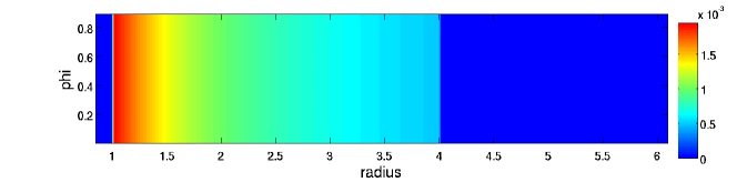
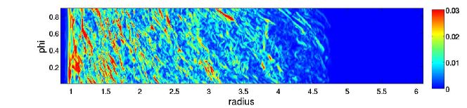
Figure 1: Panels a,b show the magnitude of the magnetic field in simulation M9d at times $t=0$ and $t=500$, respectively.

To demonstrate the buffer zone more clearly, we plot the magnetic field magnitude from simulation M9d at $t=0$ and $t=500$ in panels a and b of Fig. 1. In panel a, the field decays $\propto 1/\varpi$ between the star at $\varpi=1$ and the buffer zone at $\varpi=\varpi_{\text{B,max}}=4$. In the region $\varpi_{\text{B,max}}<\varpi<\varpi_{\text{out}}$, the field is initially set to zero. In panel b, magnetic field has penetrated into the buffer zone, as a result of the natural evolution of the MHD equations, but has not yet reached the outer boundary. In general, simulations implementing OBC1 are stopped before the magnetic field can diffuse through the buffer zone and reach the outer boundary. This allows us to run simulations for a long time, without having to worry about the effect of magnetic field at the outer boundary on the rest of the simulation domain.

label	B type	outer BC	$\varpi$-range	$N_{\varpi}$	$N_{z}$	$t_{\text{run}}$
M9a	NVF	OBC0	(.85, 6.1)	4096	128	450
M9b	NAF	OBC0	(.85, 7.85)	6144	64	450
M9c	ZNF	OBC0	(.85, 6.1)	4096	128	450
M9d	NVF	OBC1	(.85, 6.1)	4096	64	800
M9e	NAF	OBC1	(.85, 6.1)	4096	48	1000
M9f	ZNF	OBC1	(.85, 6.1)	4096	64	1800

Table 1: Summary of simulation parameters for MHD simulations. The columns from left to right are: simulation label, initial field geometry (net vertical flux, net azimuthal flux, or zero net flux), outer boundary condition, radial extent of the simulation domain, number of grid points in the radial direction, number of grid points in the vertical direction, and the total time for which the simulation was run.

3 Angular Momentum Transport: Equations

In this section, we introduce the notation used throughout this paper when discussing angular momentum transport. When analyzing simulation results, we perform both density weighted and volume weighted averages of quantities over the $z$ and $\phi$ directions. A volume weighted average is denoted by an overline:

$$\overline{f}\equiv\frac{1}{\Delta z\Delta\phi}\int dzd\phi f,$$ (11)

where $\Delta z$ and $\Delta\phi$ are the extents of the simulation domain in the $z$ and $\phi$ dimensions respectively. A density weighted average is denoted by angle brackets:

$$\langle f\rangle\equiv\frac{1}{\Delta z\Delta\phi\Sigma_{0}}\int dzd\phi\rho f,$$ (12)

where $\Sigma_{0}=\overline{\rho}$ is the volume weighted average density.

For ideal MHD, the one dimensional equation of angular momentum transport can be formulated in terms of density weighted and volume weighted averages as (Balbus & Papaloizou, 1999)

$$\frac{\partial}{\partial t}\left(\varpi^{2}\Sigma_{0}\Omega\right)+\frac{1}{\varpi}\frac{\partial}{\partial\varpi}\left(\varpi^{3}\Omega\Sigma_{0}\langle v_{\varpi}\rangle+\varpi^{2}\overline{T_{\varpi\phi}}\right) = 0,$$ (13)

where $\Omega\equiv\langle v_{\phi}\rangle/\varpi$ is the density-weighted angular velocity, and $T_{\varpi\phi}$ is the $\varpi$, $\phi$ component of the stress tensor

$$T_{\varpi\phi}\equiv\rho v_{\varpi}\left(v_{\phi}-\varpi\Omega\right)-\frac{B_{\varpi}B_{\phi}}{\mu}.$$ (14)

The first term in the space derivative in equation (13) equals the advected angular momentum current, $C_{A}$, divided by $2\pi$, and the second term equals the stress angular momentum current, $C_{S}$, divided by $2\pi$. For a steady state disk, $C_{A}+C_{S}=0$, although the disks in our simulations are not in steady state, and undergo temporal evolution.

The stress current, $C_{S}$, can be further decomposed into hydrodynamical and magnetic terms

$$C_{S,H}(\varpi,t) \equiv 2\pi\varpi^{2}\Sigma_{0}\langle v_{\varpi}\left(v_{\phi}-\varpi\Omega\right)\rangle$$ (15)

$$C_{S,B}(\varpi,t) \equiv -2\pi\varpi^{2}\overline{\frac{B_{\varpi}B_{\phi}}{\mu}}$$ (16)

$$C_{S} = C_{S,H}+C_{S,B}.$$ (17)

Note that $C_{S}$ includes contributions to the stress from both waves and the action of turbulence.

Finally, we define an $\alpha$ parameter to parametrize the angular momentum transport rate by turbulent viscosity. There are many possible definitions for $\alpha$, especially in the context of the BL (Narayan, 1992; Popham & Narayan, 1995), but the ones used in this work are

$$\alpha(\varpi,t) \equiv \frac{\overline{T_{\varpi\phi}}}{\overline{P}}=\frac{\overline{T_{\varpi\phi}}}{\Sigma_{0}s^{2}}$$ (18)

$$\alpha_{\nu}(\varpi,t) \equiv \frac{\overline{T_{\varpi\phi}}}{\Sigma_{0}sHd\Omega/d\ln\varpi}.$$ (19)

The first form of $\alpha$ is just the ratio of the stress to the pressure. The second is the $\alpha$ for a turbulent anomalous viscosity (Shakura & Sunyaev, 1973; Lynden-Bell & Pringle, 1974), where $H$ is the vertical scale of the problem. In an astrophysical disk, $H=s/\Omega$ and increases radially for constant $s$. Our simulations, however, are in cylindrical geometry and $H=\Delta z$, where $\Delta z$, the extent of the simulation domain in the vertical direction, is a constant.

Analogous to the splitting of $C_{S}$ into hydrodynamical and magnetic terms (equation [17]), it is useful to split $\alpha$ into hydrodynamical and magnetic components:

$$\alpha_{H}(\varpi,t) \equiv \frac{\langle v_{\varpi}\left(v_{\phi}-\varpi\Omega\right)\rangle}{s^{2}}$$ (20)

$$\alpha_{B}(\varpi,t) \equiv -\frac{\overline{B_{\varpi}B_{\phi}}}{\mu\Sigma_{0}s^{2}}$$ (21)

$$\alpha = \alpha_{H}+\alpha_{B}.$$ (22)

Although $\alpha$ is a useful parametrization of angular momentum transport by MRI turbulence in the disk, it is not applicable to transport by waves. In the latter case, the relevant quantity is $C_{S}$ (Belyaev et al., 2012b), and since angular momentum is transported by both waves and MRI turbulence in our simulations, we need to consider both $C_{S}$ and $\alpha$ when analyzing results.

Another useful parameter we refer to often when analyzing simulations is $\beta$ (equation [9]), and from now on we take

$$\beta(\varpi,t)\equiv\frac{\Sigma_{0}s^{2}}{\overline{B^{2}}/2\mu}.$$ (23)

4 Angular Momentum Transport by MRI in the Disk

In this section, we focus on angular momentum transport in the disk and show that we obtain resolved MRI turbulence in our simulations. Thus, this section serves as a check of our simulations against previous work, and the reader who is primarily interested in new results about wave transport of angular momentum may choose to skip ahead to the next section.

4.1 Magnetic Pitch Angle

The primary diagnostic we use to check that the disk reaches a resolved quasi-steady state of MRI turbulence is the magnetic pitch angle

$$\theta_{B}\equiv\frac{\sin^{-1}\left(\alpha_{B}\beta\right)}{2}.$$ (24)

Equation (24) gives an approximation for the angle of the magnetic field with respect to the $\phi$ direction if $B_{\phi}\gg B_{\varpi}$ and $B_{\varpi}\gg B_{z}$ (Guan et al., 2009). Sorathia et al. (2012) found that $\theta_{B}$ was a particularly good indicator of convergence, since it varies monotonically with resolution and converges to a value of $\theta_{B}\approx 13^{\circ}$ in resolved simulations. A similar indicator of convergence is the relation $\alpha\beta\approx 1/2$ (Guan et al., 2009; Hawley et al., 2011; Sorathia et al., 2012). However, $\alpha$ includes both hydrodynamical and magnetic stresses, whereas $\alpha_{B}$ is calculated using only magnetic stresses. We find in our simulations that the hydrodynamical stress due to waves is non-negligible in the disk, but waves do not contribute to the magnetic stress. Thus, a diagnostic based on $\alpha_{B}$ is strongly preferred to one based on $\alpha$, when assessing the convergence of MRI turbulence in a simulation that includes a BL.

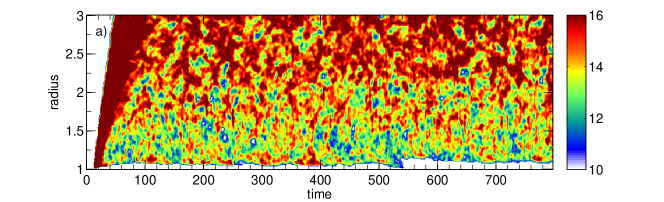
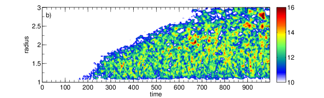
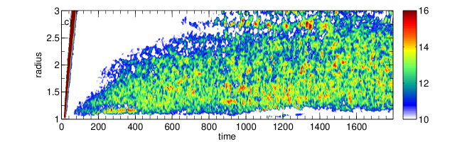
Figure 2: Panels a,b,c show $\theta_{B}$ for simulations M9d (NVF), M9e (NAF), and M9f (ZNF). The band on the left hand side of panel c is due to a transient burst of activity that occurs when the MRI first goes nonlinear. Note the different scale on the time axis in the figures.

Fig. 2 shows radius time plots of $\theta_{B}$ for simulations M9d,e,f in the annulus $1\leq\varpi\leq 3$. Ignoring the region near $\varpi=\varpi_{\star}=1$ where the rotation profile is strongly non-Keplerian, we see that $\theta_{B}\approx 12-14^{\circ}$ in the disk proper for the NAF and ZNF simulations (panels b and c) once MRI turbulence is fully developed. In the NVF simulations, $\theta_{B}\approx 12-14^{\circ}$ in the inner disk, but rises with radius. Nevertheless, the values of $\theta_{B}$ observed in our simulations are in good agreement with Sorathia et al. (2012). This gives us confidence that we have properly resolved the MRI in the disk.

4.2 Convergence Across Different Resolutions

The second diagnostic of convergence we perform is a measurement of the r.m.s. volume weighted average of $B_{\varpi}$, $B_{\phi}$, and $B_{z}$ for simulations with the same initial magnetic field geometry, but having a different resolution. Panels a,b,c of Fig. 3 show r.m.s. averages of $B_{\varpi}$, $B_{\phi}$, and $B_{z}$ at $t=400$ for NVF simulations (M9a,d), NAF simulations (M9b,e), and ZNF simulations (M9c,f), respectively. We see that the NVF and NAF simulations are converged, although the magnetic field in the outer disk of the NAF simulation is still approaching a steady state. The reason why we did not perform the convergence study at a later time is that it was too expensive to run the high resolution simulations beyond a time of $t=450$.

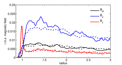
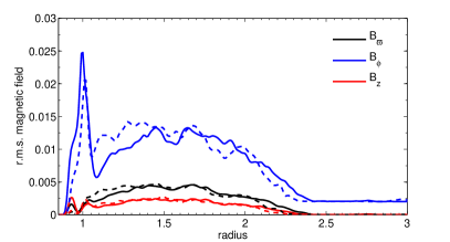
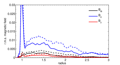
Figure 3: The volume weighted r.m.s magnetic field components at $t=400$ for NVF simulations (panel a), NAF simulations (panel b), and ZNF simulations (panel c). In each case, the solid line is the simulation with the higher z-resolution.

In the ZNF case, magnetic field components for the low resolution simulation have a higher amplitude than for the high resolution simulation, and we have checked that this is true at all times, not just at $t=400$. However, in (§4.1) we showed that MRI turbulence is resolved in ZNF simulations based on the pitch angle indicator.

Taken together, these two pieces of information suggest that MRI turbulence in our ZNF simulations is resolved, but that for a given simulation, the r.m.s field strength in the saturated state of MRI turbulence is influenced by the effective numerical viscosity and resistivity, which depend on the grid resolution (Fromang & Papaloizou, 2007). In order to make the results of ZNF simulations independent of resolution, we could add explicit viscosity and resistivity (Fromang et al., 2007).

However, given the exploratory nature of this paper, the exact value of the viscous and resistive coefficients is of secondary importance. What is more important is that for a given value of these coefficients, MRI turbulence is properly resolved, which is indeed the case according to the pitch angle indicator of §4.1.

4.3 The Value of $\alpha$ due to MRI Turbulence in the Disk

The most important parameter that characterizes transport by MRI turbulence in the disk is $\alpha$. However, $\alpha$ in our simulations is not a constant and is a function of both time and radius. One reason for this is that the timescale for instability is longer in the outer parts of the disk than in the inner parts, so the inner parts reach a quasi-steady state faster. However, even in the quasi-steady state, we find $\alpha\propto\varpi^{-3/2}$, which is not a surprising scaling, and implies a constant value of $\alpha_{\nu}$ (equation [19]). The reason $\alpha$ and $\alpha_{\nu}$ have a different radial dependence in simulations is that the height of the simulation domain, $\Delta z$ is fixed, whereas the scale height in a Keplerian disk goes as $H=s/\Omega\propto\varpi^{3/2}$ for constant $s$. Thus, we define

$$\alpha_{\text{eff}}\equiv\alpha\varpi^{3/2}.$$ (25)

Since, $s/\Omega=\Delta z$ at $\varpi=\varpi_{\star}=1$, $\alpha_{\text{eff}}$ can be thought of as the “effective” value of $\alpha$ for a Keplerian disk, based on our simulation results. The assumption here is that the angular momentum transport rate is proportional to the vertical scale of the problem, which is fixed for our simulations but goes as $H\propto\varpi^{3/2}$ for a Keplerian disk with a constant value of $s$.

Another complication to measuring the $\alpha$ due to MRI turbulence is the presence of waves emitted from the BL, which contribute to the value of $\alpha$ in the disk. Therefore, rather than showing $\alpha_{\text{eff}}$ directly, we show $\alpha_{\text{B,eff}}$, which is simply the component of $\alpha_{\text{eff}}$ that is due to magnetic stresses (i.e. $\alpha_{\text{B,eff}}=\alpha_{B}\varpi^{3/2}$). As mentioned in §4.1, $\alpha_{\text{B}}$ is insensitive to waves, which contribute primarily to the hydrodynamical stress. Studies of the MRI typically find that $\alpha\approx 5/4\alpha_{B}$ (Sorathia et al., 2012), which also roughly holds for our simulations.

Fig. 4 shows radius time plots of $\alpha_{\text{B,eff}}$ for simulations M9d,e,f. Once a quasi-steady state has been reached, the value of $\alpha_{\text{B,eff}}$ for the NVF simulation (M9d) is $\alpha_{\text{B,eff}}\approx.02-.03$, for the NAF simulation (M9e) is $\alpha_{\text{B,eff}}\approx.0075-.0125$, and for the ZNF simulation (M9f) is $\alpha_{\text{B,eff}}\approx.004-.01$. These values of $\alpha$ are consistent with those obtained by Steinacker & Papaloizou (2002) in their BL simulations. However, the value of $\alpha$ in ZNF simulations does depend on the resolution, for the same reasons as the r.m.s. magnetic field value depends on the resolution (§4.2).

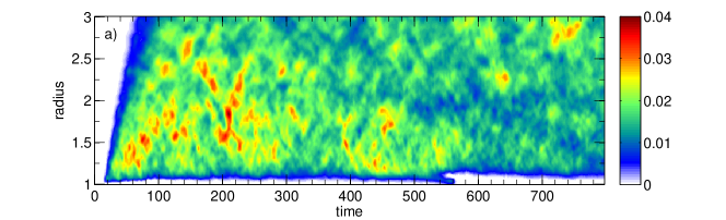
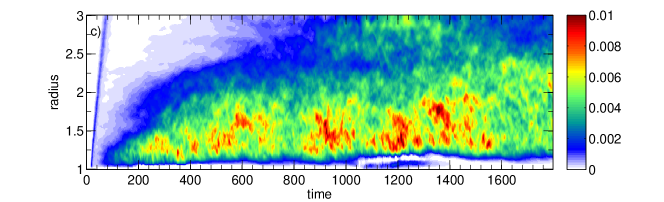
Figure 4: Panels a,b,c show $\alpha_{\text{B,eff}}$ for simulations M9d,e,f respectively. Note the different scale on the time axis in the figures.

5 Magnetic Field Amplification in the BL

It has been speculated that the strong shear present in the BL can amplify the magnetic field to the point that $\beta<1$ (Pringle, 1989). Armitage (2002) observed amplification of the field in the BL in MHD simulations with an isothermal equation of state, but found $\beta^{-1}\lesssim.1-.2$, everywhere throughout the simulation domain, including the BL. His setup assumed initial net vertical field and is most similar to our NVF model.

We also observe amplification of the $B_{\phi}$ field component in the BL in our simulations, although the amplification is highly time-variable. Referring back to Fig. 3, we see a bump in $B_{\phi}$ within the BL for the ZNF case (panel c), which clearly indicates shear amplification of the $B_{\phi}$ component. There are also bumps in $B_{z}$ and $B_{\phi}$ in panels a and b of Fig. 3, respectively. However, since panels a and b correspond to simulations having net vertical and azimuthal flux, respectively, the bump in $B_{z}$ and $B_{\phi}$ within the BL is due, at least in part, to a combination of flux freezing and compression of accreted material from the disk on the surface of the star (§7.1).

To disentangle amplification of magnetic field due to flux freezing and compression from shear amplification, we plot the maximum (in $\varpi$) of the r.m.s averaged field (in $z$ and $\phi$) as a function of time in Fig. 5 for simulations M9d,e,f. We see that the NVF and ZNF simulations (black and red curves) exhibit peaks, and the NVF simulation (black curve), in particular, has one large peak at $t\approx 560$. The NAF simulation (blue curve), on the other hand, exhibits a steady increase and contains small local peaks. The steady increase can be understood as compression of advected azimuthal field within the BL.

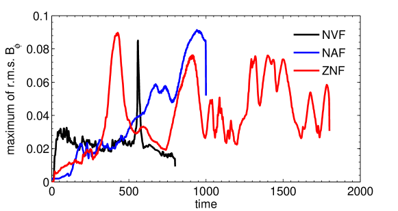
Figure 5: Plot of the maximum (in $\varpi$) of the r.m.s average (in $z$ and $\phi$) of $B_{\phi}$ as a function of time for simulations M9d,e,f (NVF, black curve; NAF, blue curve; ZNF, red curve). The spikes correspond to transient shear amplification of the $B_{\phi}$ component of the field within the BL.

The peaks in Fig. 5 are due to transient shear amplification of the field in the BL, and the baseline level in the NVF simulations (black curve) is simply set by the value of $B_{\phi}$ in the saturated state of MRI turbulence in the disk. Fig. 6 shows the r.m.s value of $B_{\phi}$ as a function of radius from simulation M9d at times $t=400$ when there is little or no amplification and $t=560$, which corresponds to the peak in the black curve in Fig. 5. From Fig. 6 it is clear that amplification of the field does indeed take place in the BL and that it is time-dependent. The cause for the time-dependency has not been explored, but it is possible that it is related to the re-excitation of acoustic modes within the BL (§7).

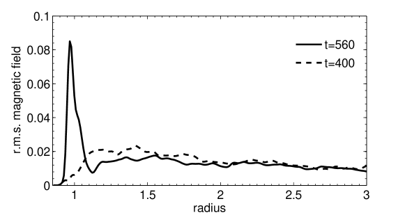
Figure 6: Plot of the r.m.s average (in $z$ and $\phi$) of $B_{\phi}$ for simulation M9d (NVF) at two different points in time. The dashed line corresponds to $t=400$ when there is little shear amplification of the magnetic field in the BL and the solid line to $t=560$ when shear amplification reaches a maximum in time.

Although there is field amplification in the BL in our simulations, the field always remains strongly subthermal, consistent with the findings of Armitage (2002). Fig. 7 shows radius-time plots of $\beta^{-1}$ (equation [9]) for simulations M9d,e,f, respectively. If magnetic pressure and thermal pressure are comparable, then $\beta\sim 1$ and if thermal pressure dominates magnetic pressure, $\beta\gg 1$. In the figures, $\beta^{-1}\lesssim.06$ for all time and throughout the entire simulation domain, which implies a significantly subthermal field.

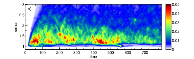
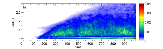
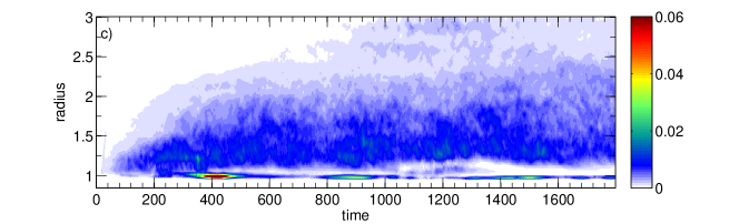
Figure 7: Panels a,b,c show radius time plots of $\beta^{-1}$ from simulations M9d,e,f respectively. There is evidence for amplification of the magnetic field in the BL, but the field remains strongly subthermal.

6 Acoustic Modes in the MHD context

Before beginning a discussion of angular momentum transport by waves in the BL and the star, we first show that waves are indeed present in our simulations. The waves being referred to are the MHD analogs of the acoustic modes discussed by Belyaev et al. (2012a, b) in the hydrodynamical case. We start by discussing how the hydrodynamical dispersion relation is modified in the presence of a magnetic field and then discuss simulation results.

6.1 Modification to the Hydrodynamical Dispersion Relation

Belyaev et al. (2012b) found that for the isothermal BL, there were three branches of acoustic modes, and they found dispersion relations that matched simulation results for each of these three branches. However, their results were for the pure hydro case, and we comment on how they should be modified to account for the presence of a magnetic field in the disk.

It is natural to expect that the major modification to the dispersion relation of the acoustic modes in the limit of $\beta\gg 1$ is the replacement of the sound speed with the magnetosonic speed.

$$v_{\text{ms}} = \sqrt{s^{2}+v_{A}^{2}}$$ (26)

$$= s\sqrt{1+\frac{2}{\gamma}\beta^{-1}}$$ (27)

where $v_{A}$ is the Alfvén speed, and $\gamma=1$ for an isothermal equation of state.

In reality, the situation is slightly more complicated, and the dispersion relation depends on the jump in magnetic field across the BL. We show this explicitly in Appendix A, where we derive an analytic dispersion relation for the 2D modes of a compressible vortex sheet (Miles, 1958; Gerwin, 1968; Belyaev & Rafikov, 2012) in the presence of a magnetic field that is perpendicular to the plane of the modes. This is not a realistic setup, but it highlights how the hydrodynamical dispersion is modified when a magnetic field is introduced.

The main result of the analysis, in the context of astrophysical BLs, is that in the limit of $\beta\gg 1$, the dispersion relation for the model system is only modified by terms of $\mathcal{O}\left(\beta^{-1}\right)$. This result, which may be expected to hold for more general field configurations, shows that when gas pressure dominates magnetic pressure, acoustic modes should still be present, and their properties should only be slightly modified as compared to the hydro case. In a typical astrophysical context, such as in MRI turbulence, the magnetic field is subthermal, meaning $\beta>1$. As we have shown in §5, the same is also true inside the BL, meaning that the modes present in the layer and its vicinity are essentially acoustic modes, weakly modified by a magnetic field.

In addition to magnetosonic waves, an ideal fluid in the presence of a magnetic field also supports Alfvén and slow waves. One may wonder whether there are also modes of the system that correspond to a coupling of these waves in the disk across the BL to either gravity or sound waves in the star. This subject is beyond the scope of the present work. However, we mention that in our simulations, the modes that show up most clearly are the analogs of the acoustic modes discussed by Belyaev et al. (2012a, b). Thus, it is natural to expect that these magnetosonic modes are the most important ones for transporting angular momentum in the presence of a magnetic field, when $\beta\gg 1$.

6.2 Simulation Results

We observe excitation of magnetosonic modes in our simulations, which persist, typically, for the duration of the simulation. Fig. 8 shows both the simple vertical average and the cross-section through the $z=0$ plane of both $\varpi\sqrt{\rho}v_{\varpi}$ and the magnetic field magnitude for simulation M9f at time $t=1000$. The dominant mode in Fig. 8 is the $m=14$ lower branch mode. It appears prominently in $\varpi\sqrt{\rho}v_{\varpi}$ (panels a and b), but only weakly in the magnetic field magnitude (panels c and d). The measured pattern speed of the $m=14$ mode from simulations is $\Omega_{P}\approx.4$, which is in good agreement with the theoretically predicted pattern speed for the $m=14$ lower branch mode, $\Omega_{P}=.415$ (Belyaev et al., 2012b).

We also point out that the mode depicted in Fig. 8 is effectively two-dimensional, since there is not much difference between the vertically averaged image of $\varpi\sqrt{\rho}v_{\varpi}$ (panel a) and the cross-sectional slice (panel b). The magnetic field, on the other hand, exhibits much more vertical structure (panels c and d), which is indicative of turbulence.

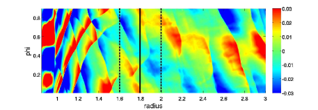
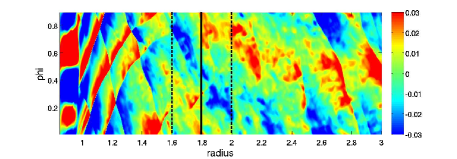
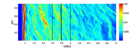
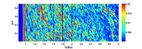
Figure 8: Snapshots at $t=1000$ from simulation M9f. Panel a) shows the simple vertical average of $\varpi\sqrt{\rho}v_{\varpi}$, and b) shows a slice through the $z=0$ plane of $\varpi\sqrt{\rho}v_{\varpi}$. Panel c) shows the simple vertical average of the magnetic field magnitude and d) shows a slice through the $z=0$ plane of the magnetic field magnitude. The dashed lines mark the edges of the evanescent region for the $m=14$ lower branch mode, and the solid line marks the location of the corotation radius in the disk for that mode.

The lower branch has an evanescent region in the disk around the corotation radius and waves incident on the evanescent region are reflected back towards the BL. The edges of this evanescent region are located approximately at the Lindblad radii, which are implicitly defined by the condition $\Omega(\varpi_{\text{LR}})=\Omega_{P}\pm\kappa(\varpi_{\text{LR}})/m$, where $\kappa$ is the epicyclic frequency. The dashed lines in Fig. 8 show the edges of the evanescent region, as predicted by hydrodynamical theory assuming a Keplerian rotation profile, and the solid line shows the corotation radius of the mode in the disk. Even though we now have MRI turbulence in the disk, shocks still reflect off inner edge of the evanescent region. This fact, together with the agreement between the measured pattern speed and that from hydrodynamical theory, means hydrodynamical theory provides a good description of the properties of magnetosonic modes even in the presence of MRI turbulence in the disk. As argued earlier, this can be attributed to the fact that $\beta^{-1}\ll 1$ in the simulations, so the magnetic field does not significantly affect the properties of acoustic modes.

Although the hydrodynamical and MHD cases exhibit many similarities, some differences are apparent. The first difference is that MHD simulations are typically “noisier” than hydro runs (Belyaev et al., 2012a, b) with a superposition of modes present. The second difference is that unlike the hydrodynamical case, there can be significant wave action tunneling through the evanescent region in MHD runs.

The presence of a superposition of acoustic modes in the disk is a generic feature, independent of initial magnetic field geometry. In addition to the lower branch, which is persistent in all of our simulations for $t\gtrsim 60$, we also observe the upper branch at the beginning of some simulations, but only in transience. Fig. 9 shows the upper branch at $t=40$ in simulation M9c. The mode depicted in the figure has $m=14$ and a measured pattern speed of $\Omega_{P}=.84$. This agrees well with the theoretically predicted pattern speed for this mode, which is $\Omega_{P}=.87$.

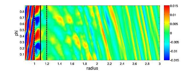
Figure 9: Image of the simple vertical average of $\varpi\sqrt{\rho}v_{\varpi}$ at $t=40$ for simulation M9c. The $m=14$ upper branch mode is clearly present in the image. The magnetic field is not shown, since at this time, the MRI instability has not yet fully developed. The dashed lines mark the edges of the evanescent region for the $m=14$ upper mode, and the solid line shows the corotation radius for that mode.

7 Angular Momentum Transport by Waves in the BL, Star, and Inner Disk

Having shown that magnetosonic modes are present in our simulations and have similar properties to the acoustic modes discussed in Belyaev et al. (2012b), we now show that they are able to transport angular momentum in the star and inner disk just as in hydrodynamical simulations.

7.1 Density Gap in the Inner Disk and Accretion onto the Star

We begin our discussion of wave transport of angular momentum by showing the evolution of the density profile. Fig. 10 shows radius time plots of $\Sigma_{0}(\varpi,t)$ in simulations M9d,e,f. In each case, a gap in the density develops in the inner disk in the vicinity of the BL ($\varpi\gtrsim 1$). The gap is opened up relatively rapidly, over a time of $\lesssim 10$ orbits, and in panels a and c, gap formation is followed at a later time by gap deepening. Concentrating on panel c, after the initial gap opening event at $t\approx 200$, the density profile of the gap stays approximately constant, until $t\approx 1100$ when it undergoes substantial gap deepening. For $t>1100$, the gap is gradually filled in by the action of turbulent viscosity in the disk.

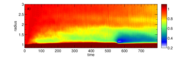
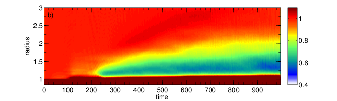
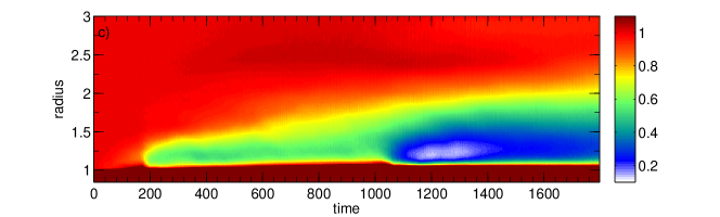
Figure 10: Panels a,b,c show radius time plots of $\Sigma_{0}$ from simulations M9d,e,f (NVF, NAF, ZNF) respectively. A density gap in the disk near $\varpi=1$ develops in all of the simulations and in panels a and c gap deepening is observed at a later time.

Belyaev et al. (2012b) also observed gap formation in their hydrodynamical simulations, which was driven by angular momentum transport by acoustic modes. Consistent with their results, we find that magnetosonic modes are responsible for opening up the gap in our MHD simulations, and we discuss the link between acoustic modes and the gap in the inner disk in more detail in §7.2.

Material gets removed from the inner part of the disk between the BL and the wave reflection point at the inner Lindblad resonance by the action of magnetosonic modes. In this region gas orbits the star faster than the pattern of acoustic modes, and every time a fluid element encounters a weak shock (into which modes evolve) it loses angular momentum and moves towards the star, giving rise to continuing accretion. Fig. 11 shows plots of the instantaneous mass accretion rate through radius $\varpi$, $\dot{M}(\varpi)$, for simulations M9d,e,f (panels a,b,c) and for a $M=9$ hydro simulation from Belyaev et al. (2012b) (panel d). The solid curves correspond to periods when magnetosonic/acoustic modes are excited to a high amplitude (high shock accretion rate) and the dashed curves to periods when their amplitude is not as high (low shock accretion rate). Each of the solid curves in panels a-c corresponds to one of the gap formation or opening events in Fig. 10.

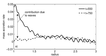
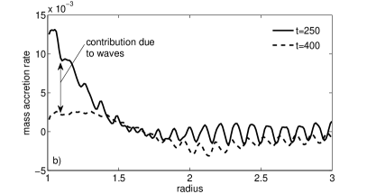
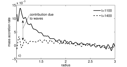
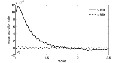
Figure 11: Panels a, b, c show plots of the instantaneous mass accretion rate, $\dot{M}$, from simulations M9d,e,f (NVF, NAF, ZNF) at the times indicated in the legends. Panel d shows the mass accretion rate for an $M=9$ hydro simulation considered in Belyaev et al. (2012b) (their 3D9a simulation). The solid and dashed lines show $\dot{M}$ during periods when acoustic modes have relatively high and low amplitudes, respectively. The large spike in accretion rate in the inner disk for the solid curves as compared to the dashed ones is caused by shock accretion in the inner disk due excitation of modes to a high amplitude.

In panels a-c, the dashed and solid curves converge to approximately the same value of $\dot{M}$ in the outer disk in Fig. 11, but the solid curves have a significantly higher amplitude than the dashed ones in the inner disk ($\varpi\gtrsim 1$). The extra contribution to $\dot{M}$ for the solid curves in the inner disk in panels a-c is provided by magnetosonic modes, and the base level of $\dot{M}$ in the outer disk is due to MRI turbulence.

Evidence for this assertion is provided by considering panel d of Fig. 11. Since the simulation corresponding to panel d is hydrodynamical, there is no MRI in the disk. This explains why the dashed line is everywhere approximately zero, since in the absence of waves excited to a high amplitude or MRI, there is no efficient mechanism for angular momentum transport in the disk. On the other hand, the shape and amplitude of the solid curve in the inner disk in panel d are similar to those of the solid curves in panels a-c. This shows that in the MHD case, the mass accretion rate in the inner disk due to shocks can dominate that due to MRI, during periods when modes are excited to a high amplitude.

Indeed, we can write the following expression for the combined mass accretion rate close to the star (interior to the evanescent region in the disk) driven by both the MRI and shocks:

$$\dot{M}=\frac{\Sigma s^{2}}{\Omega}\left[4\pi\alpha q\frac{\partial\ln\left(\alpha qs^{2}\Sigma\varpi^{2}\right)}{\partial\ln\varpi}+\frac{m}{3(2-q)}\left(1+\frac{\Delta\Sigma}{\Sigma}\right)^{-2}\left(\frac{\Delta\Sigma}{\Sigma}\right)^{3}\right],$$ (28)

where $q(\varpi)\equiv-d\ln\Omega/d\ln\varpi$ is the local shear rate ($q=3/2$ for a Keplerian disk but is a function of $\varpi$ for a general rotation profile), $m$ is the azimuthal wavenumber of the mode, and $\Delta\Sigma/\Sigma$ is the density contrast across the shock (mode) fronts. The first term in brackets is the contribution from MRI ($\alpha$ here is solely due to MRI) and can derived using the results of Lynden-Bell & Pringle (1974) and Rafikov (2012). The second term is the contribution from magnetosonic waves following from Belyaev et al. (2012a), namely from their equation (B7). For a characteristic azimuthal wavenumber of $m\sim 15-30$ and MRI viscosity $\alpha\lesssim 10^{-2}$ (see Fig. 4) measured in our simulations, one finds that both transport mechanisms provide comparable contribution to $\dot{M}$ if $\Delta\Sigma/\Sigma\sim 0.2$.

However, during periods of strong wave excitation $\Delta\Sigma/\Sigma$ increases and the wave term strongly dominates $\dot{M}$ because of the steep (cubic) dependence of $\dot{M}$ upon $\Delta\Sigma/\Sigma$. For instance, the amplitude of the $m=14$ magnetosonic mode changes by a factor of $\approx 5$ in simulation M9f between $t=900$ and $t=1100$. This results in a predicted mass accretion rate due to shocks in the inner disk that is higher by approximately two orders of magnitude at $t=1100$ as compared to $t=900$.

This effect of enhanced mass accretion rate by shocks during periods when magnetosonic modes are excited to a high amplitude is demonstrated by the solid curves in Fig. 11. Equation (28) also explains the characteristic spatial dependence of $\dot{M}$ on $\varpi$: approximate conservation of the wave angular momentum flux (neglecting for the moment dissipation at the shock fronts) results in (see equation (25) of Belyaev et al. (2012a))

$$\frac{\Delta\Sigma}{\Sigma}\propto\left[\frac{|\Omega(\varpi)-\Omega_{P}|}{\Sigma s^{3}\varpi}\right]^{1/2}.$$ (29)

This expression shows that $\Delta\Sigma/\Sigma$ is highest near the BL, where $|\Omega(\varpi)-\Omega_{P}|$ is large and goes to zero in the evanescent region where $\Omega=\Omega_{P}$. This explains why during the high wave amplitude episodes, when mass accretion is clearly dominated by dissipation of acoustic modes, $\dot{M}$ is largest near the BL, but rapidly decays to small value as $\varpi$ approaches the evanescent region in the disk.

Note that inside the BL MRI does not operate, $\alpha=0$, and the first term in equation (28) vanishes, leaving wave dissipation as the only means of mass transport. On the other hand, in the disk outside the corotation radius, waves do not contribute to transport and second term in equation (28) disappears. Thus, MRI remains the only mass transport mechanism outside the resonant cavity in which the pattern of standing acoustic modes exists, in agreement with the picture outlined in Belyaev et al. (2012a) and Belyaev et al. (2012b).

7.2 Angular Momentum Transport due to Waves and MRI

In this section, we connect the density gap in the inner disk to magnetosonic modes and discuss angular momentum transport in the star, BL, and inner disk more generally.

Fig. 12 shows radius time plots of the angular momentum current, $C_{S}$, from simulations M9d,e,f. In the disk, far away from the BL, angular momentum transport is due primarily to MRI turbulence (§4), and $C_{S}$ is approximately constant at a given radius once the MRI has saturated. We note that the striations appearing in $C_{S}$ are caused by waves. The striations in the panels of Fig. 12 are predominantly downward sloping in the inner disk, indicating inward propagating waves. These waves are excited at the “front” of MRI turbulence which propagates radially outward through the disk over the course of the simulation. Although potentially a nuisance, these waves do not play a major role in angular momentum transport in our simulations.

In contrast to the outer disk, where the value of $C_{S}$ at a given radius is approximately constant in time once MRI turbulence has saturated, $C_{S}$ varies by more than an order of magnitude in the star and inner disk over the course of a simulation. This implies a mechanism of angular momentum transport that is decoupled from MRI turbulence. As we shall shortly demonstrate, this mechanism is transport of angular momentum by magnetosonic modes. Given this fact, we can directly link magnetosonic modes to the gap formation and deepening events in Fig. 10, since these are simultaneous with the periods when $C_{S}$ is large in the BL and star in Fig. 12.

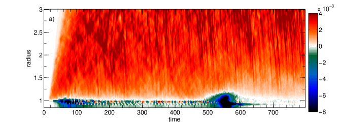
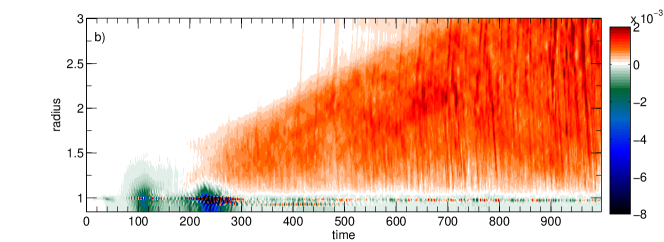
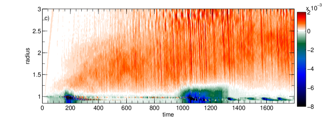
Figure 12: Panels a,b,c show radius time plots of the angular momentum current $C_{S}$ from simulations M9d,e,f (NVF, NAF, ZNF) respectively. Notice that $C_{S}$ changes sign in the vicinity of the BL with $C_{S}<0$ for $\varpi\lesssim 1$ and $C_{S}>0$ for $\varpi\gtrsim 1$.

In addition to waves dominating angular momentum transport in the star and BL, we find that they also contribute significantly to angular momentum transport in the inner disk. Fig. 13 shows $C_{S}$ and $\Omega$ superimposed on the same plot for simulations M9d,e,f at times $t=550$, 250, and 1100, when the angular momentum current due to waves is high in each simulation. The dashed vertical line denotes the radius at which $C_{S}=0$, and for an anomalous viscosity model, $C_{S}=0$ and $d\Omega/d\varpi=0$ occur at the same radius (equation [19]). However, we see in Fig. 13 that the radius at which $C_{S}=0$ is significantly displaced into the disk compared to the radius at which $d\Omega/d\varpi=0$. This implies that $C_{S}$ contains a contribution due to waves in the disk, since $C_{S}<0$ for outgoing waves up to the corotation radius in the disk, which is located at $\varpi_{\text{cr}}\approx 1.8$ ($m=14$ mode) in each of the panels in Fig. 13.

We conclude that when waves are excited to a high amplitude, they significantly modify the profile of $C_{S}$ in the inner disk compared to what is expected for a turbulent viscosity model. In particular, if both magnetosonic modes and anomalous viscosity contribute appreciably to $C_{S}$, then the radius at which $C_{S}=0$ in the disk is neither at the corotation radius of the mode, nor at the radius where $d\Omega/d\varpi=0$, but somewhere in between.

We also mention that the variation of $C_{S}$ with radius in the star and BL in each of the panels in Fig. 13 is consistent with $C_{S}(\varpi)$ for the lower branch (Fig. 12 of Belyaev et al. (2012b)). Since the lower branch is directly observed in our simulations (§6), this provides further confirmation that angular momentum is transported by waves in the BL and star.

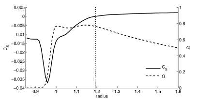
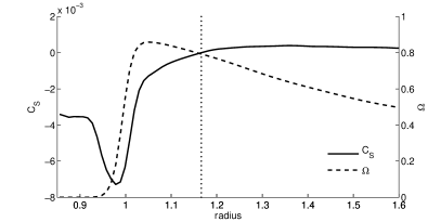
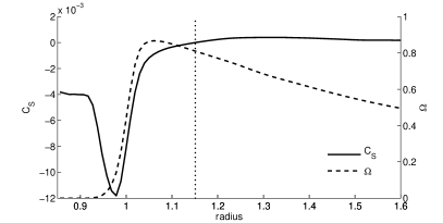
Figure 13: Panels a,b,c show plots of $C_{S}$ and $\Omega$ for simulations M9d,e,f at times $t=550$, 250, and 1100. The dashed vertical line denotes the radius at which $C_{S}=0$ and is significantly displaced into the disk relative to the radius at which $d\Omega/d\varpi=0$. In general, when angular momentum in the disk is transported by both a magnetosonic mode and turbulent viscosity, the location at which $C_{S}=0$ occurs between the radius at which $d\Omega/d\varpi=0$ and the corotation radius of the mode, $\varpi_{\text{cr}}\approx 1.8$ in this example.

7.3 Hydrodynamical Nature of Angular Momentum Transport in the Star and BL

Having established that magnetosonic modes transport angular momentum in the BL and star, and also influence transport in the inner disk, we now demonstrate that the mechanism of angular transport by acoustic modes is essentially hydrodynamical in nature. This provides evidence for the argument presented in §6.1 that when $\beta\gg 1$, the properties of acoustic modes are not significantly affected by the magnetic field, and the results of Belyaev et al. (2012b) are valid.

To show that stresses in the BL are hydrodynamical, we split $C_{S}$ into magnetic and nonmagnetic components (equation [17]). Fig. 14 shows $C_{S,B}$ and $C_{S,H}$ for each of simulations M9d,e,f, and several things are immediately apparent. The first is that $C_{S,B}$ is several times larger than $C_{S,H}$ in the disk, which is consistent with the fact that the magnetic stress is several times the hydrodynamical stress for MRI turbulence (Sorathia et al., 2012). The second is that $C_{S,B}$ vanishes going into the star and there is no bump in $C_{S,B}$ within the BL. This means that magnetic stresses are not important for transport in the BL. This is consistent with the results of Pessah & Chan (2012), who found that in the shearing sheet approximation, the magnetic stress oscillates about zero for a rising rotation profile ($d\Omega/d\varpi>0$), as in the BL. The third is that $|C_{S,H}|\gg|C_{S,B}|$ in the star and BL, which is definitive proof that a hydrodynamical mechanism of angular momentum transport operates there – namely acoustic modes weakly modified by a magnetic field.

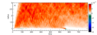
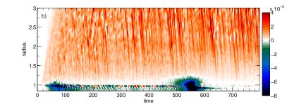
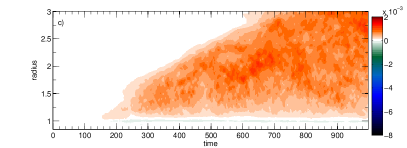
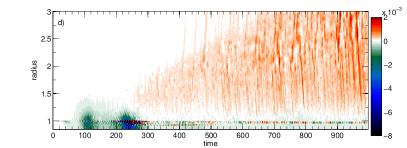
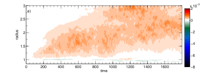
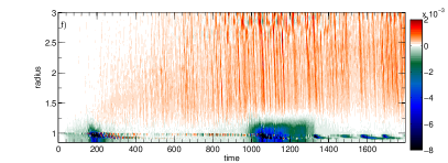
Figure 14: Panels a,c,e show radius time plots of $C_{S,B}$ from simulations M9d,e,f (NVF, NAF, ZNF) respectively, and panels b,d,f show radius time plots of $C_{S,H}$ from simulations M9d,e,f. The scale, colormap, and axes labels for each simulation (M9d,e,f) are the same as in Fig. 12. Notice that $C_{S,B}$ vanishes inside the star, and there is no bump in $C_{S,B}$ within the BL. On the other hand, $C_{S,H}$, is large inside the BL and is both large and approximately constant (spatially) within the star, which suggests transport by waves.

7.4 Boundary Layer Width

Belyaev et al. (2012a) and Belyaev et al. (2012b) found that in hydro simulations the BL settled to a radial width of $6-7$ radial scale heights ($h_{s}\equiv s^{2}/g(\varpi_{\star})$). Using their definition for the BL as the region in which

$$0.1<\langle v_{\phi}(\varpi)\rangle/v_{K}(\varpi)<0.9,$$ (30)

we confirm that after the initial gap opening event, the BL in our MHD simulations also settles down to a radial width of 6-7 radial scale heights (Fig. [15]). However, the BL undergoes widening events that are coincident with gap deepening events (§7.1) and the periods when $C_{S}$ is large in the star and BL (§7.2). Stochastic widening events were also observed by Belyaev & Rafikov (2012) in 2D hydro simulations, and it appears that in both hydro and MHD cases these events are mediated by the action of shocks on the fluid in the inner disk.

The fact that the BL widening events occur simultaneously with gap deepening events, suggests a common origin, implying that magnetosonic modes play a critical role in regulating the width of the BL. However, given the occurrence of stochastic widening events in the simulations, the width of the BL is time-variable and it is not possible to assign a single number to it. Nevertheless, what the simulations suggest is that the BL initially settles down to a steady state width of 6-7 radial scale heights and is subsequently widened, during periods when magnetosonic modes are excited to a high amplitude.

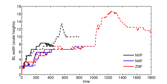
Figure 15: Boundary layer width in units of scale height $s^{-2}$ (defined implicitly in equation [30]) as a function of time, for each of our simulations. The black, blue, and red curves correspond to NVF, NAF, and ZNF simulations respectively. The solid lines correspond to simulations with the higher resolution for a given magnetic field geometry.

7.5 Physical Origin for Gap Deepening Events and Associated Phenomena

We now discuss in more detail the physical mechanism behind gap deepening events (§7.1). These events are coincident with increased angular momentum current in the vicinity of the BL (§7.2), increased mass accretion rate in the inner disk (§7.1), and BL widening events (§7.4). The physical origin of all of these phenomena appears to be re-excitation of magnetosonic modes to a high-amplitude. Although it is difficult to determine the cause of this re-excitation, it is straightforward to understand the effect it has on the flow.

Magnetosonic waves emitted from the BL steepen and shock in the disk (Fig. 8), which leads to a transfer of energy from the wave to the fluid (Goodman & Rafikov, 2001; Belyaev et al., 2012b). For weak shocks, the rate of energy dissipation in the shock per unit mass and mass accretion rate are both proportional to $(\Delta\Sigma/\Sigma_{\text{pre}})^{3}$ (Larson, 1990; Belyaev et al., 2012a), where $\Delta\Sigma\ll\Sigma_{\text{pre}}$ is the jump in density across the shock front and $\Sigma_{\text{pre}}$ is the preshock density. Since $\Delta\Sigma$ is proportional to the amplitude of the magnetosonic mode (just after it has shocked), even a modest change in the amplitude of the mode by a factor of a few results in greatly enhanced energy dissipation and mass accretion rates. For instance, the amplitude of the $m=14$ magnetosonic mode changes by a factor of $\approx 5$ in simulation M9f between $t=900$ and $t=1100$. This results in a predicted mass accretion rate due to shocks in the inner disk that is higher by approximately two orders of magnitude at $t=1100$ as compared to $t=900$.

During periods when magnetosonic modes are excited to high amplitudes, shocks in the inner disk slow down matter so efficiently that sharp density gradients appear in the BL vicinity. Associated increased radial pressure support results in a formation of a “dip” in the angular velocity profile. Panel c of Fig. 16 shows $\Omega(\varpi)$ at various times for simulation M9f. The time $t=900$ is before acoustic modes are excited to a high amplitude, $t=1100$ is the time of largest excitation, and $t=1600$ is after acoustic modes have waned in amplitude. Associating these times with panel c of Fig. 12, it is clear they correspond to the periods before, during, and after the excitation event.

The dip in the rotation profile in panel c of Fig. 16 is most prominent at $t=1100$. Notice that the dip occurs in the inner disk, beyond the region of largest shear, which occurs in the BL. This is most apparent in panels a and b of Fig. 16, which show the $z$ components of the vorticity and potential vorticity. The vorticity and potential vorticity are defined by ${\boldsymbol{\omega}}\equiv\boldsymbol{\nabla}\times\boldsymbol{v}$ and ${\boldsymbol{\omega}}_{\text{pot}}\equiv\boldsymbol{\nabla}\times\boldsymbol{v}/\Sigma$, respectively.

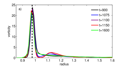
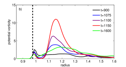
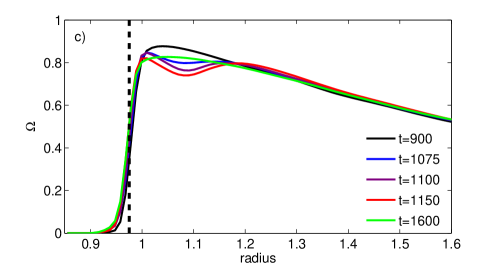
Figure 16: Panels a,b,c show plots of the vorticity, potential vorticity, and angular velocity, respectively, for simulation M9f (ZNF). The dashed black curve is the corotation resonance in the BL for the dominant mode during the period of time in question. Each of the curves corresponds to a time that is before, during, or after the period when magnetosonic modes are excited to a high amplitude ($1000\lesssim t_{\text{high}}\lesssim 1250$). The dip in the angular velocity in panel c around $t=1100$ is due to the action of shocks. This dip shows up as the second peak (with respect to radius) in panels a and b. The first corresponds to the BL.

The first of the two peaks shown in panels a and b of Fig. 16 corresponds to the BL and is suppressed in the potential vorticity as compared to the vorticity due to the rise in density into the star. The second peak corresponds to the dip in $\Omega$ shown in panel c and is enhanced in the potential vorticity as compared to the vorticity, due to the drop in density in the inner disk (e.g. Fig. 10). For reference, the corotation resonance of the $m=14$ lower branch mode within the BL, which is dominant throughout the period in question, is shown by the dashed vertical line.

The second peak in panels a and b of Fig. 16 is only prominent during the period when magnetosonic modes are excited to a large amplitude. The fact that it is well-separated from the BL, implies that magnetosonic modes transfer their energy to the fluid and drive accretion primarily through shocks in the inner disk. This is in contrast to transfer of energy and angular momentum through nonlinear wave damping at the corotation resonance, which does not appear to be a significant factor in creating the density gap in the inner disk and associated phenomena. However, we speculate that the amplitude of magnetosonic modes themselves is determined by wave-fluid interaction at the corotation resonance within the BL. Thus, it is quite possible this resonance plays an integral role in pumping magnetosonic modes up to high amplitudes, which is a prerequisite to achieving high accretion rates due to shocks in the inner disk.

8 Discussion

We have shown that even in the presence of MRI turbulence in the disk, waves dominate angular momentum transport in the BL, and influence transport in the inner disk. The importance of waves for angular momentum transport in the BL was previously shown by Belyaev et al. (2012b) for the purely hydrodynamical case.

We find that when a magnetic field is introduced, the acoustic modes discussed by Belyaev et al. (2012b) become magnetosonic modes. These magnetosonic modes have a dispersion relation that differs from the dispersion relation for acoustic modes by factors that are $\mathcal{O}(\beta^{-1})$. Since the field in our simulations is highly subthermal ($\beta^{-1}\lesssim.06$) everywhere, including the BL, the hydrodynamical theory of Belyaev et al. (2012b) remains a good approximation to the dynamics of magnetosonic modes in our simulations.

Unlike MRI turbulence, which can be parametrized by an anomalous viscosity, the transport of energy and angular momentum in the BL is a non-local process, as has been emphasized in Belyaev et al. (2012b). Energy and momentum are carried away from the BL by acoustic waves weakly modified by magnetic field into both the star and the disk and can be deposited far away from the BL. This has important implications for stellar spinup, heating of the star, disk and the BL itself, and for observational manifestations of the BL phenomenon (Belyaev et al., 2012b). In the MHD case, additional dissipation is produced in the disk due to the operation of MRI but, as one can infer from Fig. 4 where $\alpha_{B}$ is seen to vanish in the BL, the MRI-generated heat is unlikely to penetrate into the BL and affect its structure.

Amplification of the magnetic field in the BL that we see in our simulations (§5) is consistent with earlier theoretical expectations (Pringle, 1989) but does not result in efficient magnetically-mediated transport of angular momentum in this region. Our study is in agreement with the analytical work of Pessah & Chan (2012), who analyzed the evolution of MHD modes in presence of shear with $\partial\Omega/\partial\varpi>0$ and demonstrated that although the energy density of these modes can be amplified significantly, their associated stresses oscillate around zero, rendering them inefficient at transporting angular momentum. As a consequence, angular momentum transport in the BL is mediated by quasi-acoustic modes, and in particular shock dissipation of these modes in the inner disk.

Previously, Steinacker & Papaloizou (2002), Armitage (2002) performed isothermal MHD simulations of the BL, and the setup of Armitage (2002) in particular was nearly identical to ours. Therefore, a natural question that arises is why did these authors not observe acoustic modes and recognize their importance for angular momentum transport in the BL? Interestingly, the answer to this question may be that the modes were in fact observed in these early simulations, but their presence and significance were not fully appreciated.

For instance, Fig. 3 of Armitage (2002) shows an image of relative density perturbation averaged over the z-dimension. The density fluctuations in the image exhibit a leading/trailing mode pattern that looks strikingly similar to the lower mode trapped between the BL and the evanescent region in the disk, see Fig. 8. Note that $\Delta\Sigma/\Sigma\propto\Sigma^{-1/2}$ for an acoustic mode propagating into the star by angular momentum conservation, see equation (29), which explains why the amplitude of density fluctuations rapidly decreases going into the star in Fig. 3 of Armitage (2002).

It is harder to comment on whether Steinacker & Papaloizou (2002) observed acoustic modes, since they used a different initial setup than ours and prescribed a rotation profile for the BL region in their simulations. In contrast, the profile of $\Omega$ in the BL is naturally established in our simulations due to action of the sonic instability early on in the simulations (Belyaev et al., 2012a, b), which widens the initial interfacial region into a self-consistent BL. Nevertheless, it is quite possible that Steinacker & Papaloizou (2002) also observed acoustic modes excited in the BL, as they briefly mentioned the presence of “stochastic spiral patterns” in their simulations, which could well have been the manifestation of acoustic modes (e.g. see Fig. 7 of Steinacker & Papaloizou (2002)).

Another important question that arises is given that we have used an isothermal equation of state, what might be expected for a more realistic equation of state? As discussed in Belyaev et al. (2012b) one pathology of the isothermal equation of state is that the Brunt-Väisälä frequency, $N^{2}=(\gamma-1)g^{2}/s^{2}$, is equal to zero. This means that our computational model does not support gravity waves and in a real star with nonzero Brunt-Väisälä frequency, magnetosonic waves in the disk could couple to gravity waves in the star increasing the number of possible modes in the star-BL-disk system.

Another difference is that the sound speed is not constant in a real star and is an inverse function of the radius. This means that the cutoff frequency below which sound waves do not propagate is also an inverse function of the radius and without a damping process, such as radiative damping, waves propagating into the star would reflect back towards the BL. A simple way to model this effect in simulations would be to introduce a reflecting wall at the inner boundary of the simulation domain. Glatzel (1988), Belyaev & Rafikov (2012) found analytically that for the case of a supersonic shear layer with a linear velocity profile, instability was present for both reflecting wall and radiation boundary conditions. Therefore, although reflection at an inner boundary would likely modify the details of angular momentum transport by waves, in particular the spinup rate of the star and possibly the wavelength of the dominant mode, magnetosonic modes would still be excited in such a system.

Appendix A Dispersion Relation for the Compressible Vortex Sheet in the Presence of a Constant Magnetic Field that is Oriented Perpendicular to the Motion

Here we present the dispersion relation for modes of the compressible vortex sheet with wavevectors lying in the $x$-$y$ plane, when a $z$-directed magnetic field is present. Under this set of assumptions, the $\boldsymbol{B}\cdot\boldsymbol{\nabla}\boldsymbol{B}$ term in the MHD equations is zero, which means Alfvén waves are not permitted, the slow wave is null, and only the fast magnetosonic wave survives. In fact, in such a setup the magnetic field simply provides pressure support and behaves as though it were a fluid with an effective adiabatic index of $\gamma_{B}=2$. Although this is not a realistic description for astrophysical boundary layers, it gives us a flavor for how the dispersion relation of acoustic modes is modified when a weak magnetic field is introduced. In particular, it shows that for a weak magnetic field, the corrections to the dispersion relation are small and are of order $\mathcal{O}\left(\beta^{-1}\right)$.

Since all fluid quantities in our setup are independent of $z$ we are essentially studying a 2D problem. In that case, the ideal MHD equations with an adiabatic equation of state can be formulated as

$$\frac{\partial\rho}{\partial t}+\boldsymbol{\nabla}\cdot(\rho\boldsymbol{v}) = 0,$$ (A1)

$$\frac{\partial(\rho\boldsymbol{v})}{\partial t}+\boldsymbol{\nabla}\cdot(\rho\boldsymbol{v}\boldsymbol{v}) = -\boldsymbol{\nabla}\left(P+\frac{B_{z}^{2}}{2\mu}\right),$$ (A2)

$$P = K\rho^{\gamma},$$ (A3)

$$B_{z} = \sigma\rho,$$ (A4)

where, we have replaced the induction equation (3) with the frozen-in law (A4) and introduced the “magnetization” of the fluid per unit mass, $\sigma$. Equations (A1-A4) can be simplified to

$$\frac{\partial\rho}{\partial t}+\boldsymbol{\nabla}\cdot(\rho\boldsymbol{v}) = 0,$$ (A5)

$$\frac{\partial(\rho\boldsymbol{v})}{\partial t}+\boldsymbol{\nabla}\cdot(\rho\boldsymbol{v}\boldsymbol{v}) = -\boldsymbol{\nabla}\left(K\rho^{\gamma}+\frac{\sigma^{2}}{2\mu}\rho^{2}\right).$$ (A6)

Written in this form, it is clear that for our setup the magnetic field behaves in the same manner as a fluid with $\gamma_{B}=2$.

We now describe the compressible vortex sheet setup, following the notation of Belyaev & Rafikov (2012). The velocity profile of the model setup is given by

$$V_{y}(x)=\left\{\begin{array}[]{lr}\bar{V}_{y},\ x>0\\ -\bar{V}_{y},\ x<0,\end{array}\right.$$ (A9)

where $\bar{V}_{y}$ is a constant, and a velocity discontinuity is present at $x=0$. For $x>0$, the density, magnetization, and sound speed are constant and are given by $\rho_{+}$, $\sigma_{+}$, and $s_{+}$, respectively. Similarly, for $x<0$ these parameters are constant as well and are given by $\rho_{-}$, $\sigma_{-}$, and $s_{-}$, respectively.

Using the techniques laid down in (Gerwin, 1968; Alexakis et al., 2002; Belyaev & Rafikov, 2012), it is a straightforward if lengthy exercise to derive the dispersion relation for linearized perturbations of this system. Thus, we omit the derivation and simply state the dispersion relation, which is

$$\epsilon^{2}\left[(M_{\text{ms}}+\varphi)^{2}\epsilon^{-1}(1+\delta)^{-1}-1\right]\left(M_{\text{ms}}-\varphi\right)^{4}=\left[(M_{\text{ms}}-\varphi)^{2}-1\right]\left(M_{\text{ms}}+\varphi\right)^{4}.$$ (A10)

Here, $\epsilon\equiv\rho_{+}/\rho_{-}$ is the density contrast across the vortex sheet, $\varphi\equiv\omega/k_{y}s_{+}$ is the dimensionless phase speed, $M_{\text{ms}}\equiv\bar{V}_{y}/\sqrt{s_{+}^{2}+v_{A,+}^{2}}$ is the magnetosonic Mach number, and $\delta$ is defined through the relation

$$\epsilon(1+\delta) = \frac{s_{-}^{2}+v_{A,-}^{2}}{s_{+}^{2}+v_{A,+}^{2}}.$$ (A11)

As in the text, $v_{A}$ denotes the Alfvén velocity.

Equation (A10) is identical to equation (39) of Belyaev & Rafikov (2012) for the unmagnetized case, except that the Mach number has been replaced by the magnetosonic Mach number, and there is an additional factor of $(1+\delta)^{-1}$. The first of these modifications, the replacement of the Mach number with the magnetosonic Mach number, is to be expected and was argued for in the text. The second is harder to anticipate and a nonzero $\delta$ can be thought of as coming from a difference in the effective $\gamma$ of the fluid across the vortex sheet. The effective $\gamma$ of the fluid is a suitably weighted combination of $\gamma$ and $\gamma_{B}$.

The major point of equation (A10) as regards astrophysical BLs is to show that for a weak magnetic field, the dispersion relation for the compressible vortex sheet is only modified up to terms of $\mathcal{O}\left(v_{A}^{2}/s^{2}\right)$ (i.e. $\mathcal{O}\left(\beta^{-1}\right)$). Since the dispersion relation for the three wave branches of acoustic modes discussed in §6 is simply related to the dispersion relation for the compressible vortex sheet (Belyaev et al., 2012a), we reason that properties of acoustic modes are also only modified by terms of $\mathcal{O}\left(\beta^{-1}\right)$ in the presence of a magnetic field. Since $\beta$ tends to be large in our simulations, even in the BL, we reason that the magnetic field due to MRI perturbs the acoustic modes, but does not modify them in a fundamental way.

It is possible that our NVF and NAF simulations would also exhibit re-excitation of magnetosonic modes if we were to run them for longer. Ultimately, however, re-excitation cannot occur indefinitely without replenishment of the material in the inner disk. This is because each excitation of the acoustic modes further depletes the gap in the inner disk, and eventually the inner disk becomes completely depleted of material. Since the density gap is opened up very quickly (in $\lesssim 10$ orbits), it is likely that excitation events occur on the timescale for material from the outer disk to replenish the density gap. This is of order the viscous timescale for the MRI turbulence in the disk, $t_{\nu}\equiv\Delta_{\varpi}^{2}/\nu_{\text{turb}}$, where $\Delta_{\varpi}$ is the width of the density gap. Using equation() for $\nu_{\text{turb}}$, the viscous timescale in our simulations is $t_{\nu}\sim 8000(\Delta_{\varpi}/\varpi_{\star})^{2}(.01/\alpha)$. This is beyond the reach of our simulations, and we would need an order of magnitude speed up to study the gap filling process and re-excitation of acoustic modes at the same resolution as used here.

In this work, we have discussed angular momentum transport in the BL by acoustic modes in the presence of a magnetized disk with MRI turbulence. One natural question that arises is why weren’t these modes observed before by Armitage (2002) or Steinacker & Papaloizou (2002). Interestingly, the answer to this question may be that the modes were in fact observed in these early simulations, but their importance for angular momentum transport was not fully realized.

For instance, Fig. 3 of Armitage (2002) shows an image of $\delta\Sigma/\Sigma_{0}$ averaged over the z-dimension. The density fluctuations in the image exhibit a pattern that looks strikingly similar to the “lower mode” discussed in this work and by Belyaev et al. (2012a). Note that $\delta\Sigma/\Sigma_{0}\propto\Sigma_{0}^{-1/2}$ for an acoustic mode propagating into the star by angular momentum conservation which explains why the amplitude of density fluctuations rapidly decreases going into the star in Fig. 3 of Armitage (2002).

It is harder to comment on whether Steinacker & Papaloizou (2002) observed acoustic modes, since they used a different initial setup than ours that prescribed a rotation profile for the BL region in their simulations. In contrast, the BL in our simulations is self-consistently established due to action of the sonic instability early on in the simulations which widens the initial interfacial region into a self-consistent BL. Nevertheless, it is quite possible that Steinacker & Papaloizou (2002) observed acoustic modes excited in the BL, as they briefly mentioned the presence of “stochastic spiral patterns” in their simulations, which could well have been the manifestation of acoustic modes (e.g. see Fig. 7 of Steinacker & Papaloizou (2002)).

Thus, we emphasize that it is not that we have done anything special to amplify the presence of acoustic modes in our simulations. Rather, these acoustic modes are self-consistently generated and should be present in any simulation of the BL with a supersonic drop in azimuthal velocity across it regardless of the details of the simulation. It seems plausible that previous studies observed these modes, but simply did not comment on their importance for angular momentum transport within the BL.

One possible explanation why the waves only operate at a large amplitude for short periods of time in our simulations is that the waves are self-regulating. Their amplitude diminishes after they open up the density gap in the inner disk, since if they were to keep the same amplitude, they would entirely deplete the inner disk of material. Subsequently, it is possible that the amplitude of the waves is set by accretion rate of material from the outer to the inner disk due to the action of MRI turbulence. At this point, this is only a conjecture since our simulations are not run for long enough to observe significant filling of the inner gap.

A.1 Relation to Previous Work

The computational techniques and methodology we use in this paper are similar to those adopted in Armitage (2002); Steinacker & Papaloizou (2002); Belyaev et al. (2012a, b). Consequently, we will leverage the results of those papers heavily in our work, and we take a moment to discuss the context of our paper in relation to these publications.

Armitage (2002) and Steinacker & Papaloizou (2002) both studied magnetic boundary layers using 3D MHD simulations in cylindrical geometry with an isothermal equation of state. Thus, the numerical model and methodology used by those authors is similar to the one we use here. Armitage (2002) was primarily interested with the amplification of the toroidal component of the field in the boundary layer by the large shear generated there, and Steinacker & Papaloizou (2002) were primarily interested in calculating transport coefficients for the BL and studying diffusion of magnetic flux into the BL. In this paper, we touch on both of these topics, and because a decade has passed since these last studies were performed, we are able to use a significantly higher resolution than these authors due to the increase in computational power. However, we do not perform a resolution study in this paper. Rather, we run the simulations at the maximum possible resolution and leverage the results of Armitage (2002); Steinacker & Papaloizou (2002) where appropriate to comment on convergence.

Nevertheless, our work is not simply a rehashing of what has been done by Armitage (2002); Steinacker & Papaloizou (2002) at a higher resolution - far from it. Belyaev et al. (2012a, b) have shown that nonaxisymmetric acoustic modes excited in the BL by shear instabilities can effectively transport angular momentum. Thus, the primary focus of this work is understanding whether these acoustic modes can survive if MRI turbulence is present in the disk and whether they are still important for angular momentum transport in the BL if the disk is magnetized. The answer to both questions, we find, is yes.

Appendix B Derivation of $\alpha-\beta$ Relation

We derive the relation (LABEL:alphabetaeq) up to constants of order unity. We begin by writing the MHD turbulent stress as

$$\tau_{\varpi\phi}=\overline{\rho\delta v_{\varpi}\delta v_{\phi}-\frac{B_{\varpi}B_{\phi}}{\mu}},$$ (B1)

where the first term is the Reynold’s stress, the second term is the magnetic stress and the overline denotes a simple average over $\phi$ and $z$. The first assumption we make is that the Reynold’s stress is some fraction $f<1$ of the magnetic stress. This is reasonable and simulations yield $f\sim 1/3-1/4$. Equation (B1) can then be written as

$$\tau_{\varpi\phi}=-(1+f)\overline{\frac{B_{\varpi}B_{\phi}}{\mu}}.$$ (B2)

Next, we assume that the magnetic stress is a fraction $g<1$ of the square of the magnetic field strength and that the magnetic stress is positive (outward transport). In this case, equation (B2) becomes

$$\tau_{\varpi\phi}=g(1+f)\overline{\frac{B^{2}}{\mu}}.$$ (B3)

From now on, we omit the overline for simplicity, and write

$$\tau_{\varpi\phi}=g(1+f)\frac{B^{2}}{\mu}.$$ (B4)

Now, the viscous stress can be expressed as

$$\tau_{\varpi\phi}=-\nu\rho\varpi\frac{d\Omega}{d\varpi}.$$ (B5)

Assuming a turbulent viscosity, $\nu_{\text{turb}}$, in the form (18), and equating the stresses in equations (B5) and (B4), we can write

$$g(1+f)\frac{B^{2}}{\mu}=-\alpha sH\rho\frac{d\Omega}{d\ln\varpi}.$$ (B6)

Equation (B6) can be written in terms of $\beta$ (equation [9]) as

$$2g(1+f)\beta^{-1}\left(-\frac{d\ln\Omega}{d\ln\varpi}\right)^{-1}=\alpha H\left(\frac{\Omega}{s}\right).$$ (B7)

For a Keplerian disk, this is

$$\frac{4g(1+f)}{3}\beta^{-1}=\alpha H\left(\frac{\Omega}{s}\right).$$ (B8)

Now, if as in a real disk we have $H=s/\Omega$, then we have

$$\frac{4g(1+f)}{3}\beta^{-1}=\alpha,$$ (B9)

which implies that $4g(1+f)/3\approx 1/2$, if we are to have $\alpha\approx\beta^{-1}/2$ as found by (citations). However, if we have as in the simulations $H=\Delta z$, where $\Delta z$ is a constant, then the right hand side of equation (B9) cannot be simplified, and the proper relation is

$$\frac{4g(1+f)}{3}\beta^{-1}=\alpha\Delta z\left(\frac{\Omega}{s}\right).$$ (B10)

Setting $4g(1+f)/3\approx 1/2$, we arrive at equation (LABEL:alphabetaeq).

References

- Alexakis et al. (2002) Alexakis, A., Young, Y., & Rosner, R. 2002, Phys. Rev. E, 65, 026313
- Armitage (2002) Armitage, P. J. 2002, MNRAS, 330, 895
- Balbus & Hawley (1991) Balbus, S. A., & Hawley, J. F. 1991, ApJ, 376, 214
- Balbus & Hawley (1992) Balbus, S. A., & Hawley, J. F. 1992, ApJ, 400, 610
- Balbus & Papaloizou (1999) Balbus, S. A., & Papaloizou, J. C. B. 1999, ApJ, 521, 650
- Belyaev & Rafikov (2012) Belyaev, M. A., & Rafikov, R. R. 2012, ApJ, 752 115
- Belyaev et al. (2012a) Belyaev, M. A., Rafikov, R. R., & Stone, J. M. 2012, ApJ, 760, 22
- Belyaev et al. (2012b) Belyaev, M. A., Rafikov, R. R., & Stone, J. M. 2012, arXiv:1212.0580
- Chandrasekhar (1960) Chandrasekhar, S. 1960, Proc. Natl. Acad. Sci., 46, 253
- Coleman et al. (1995) Coleman, C. S., Kley, W., & Kumar, S. 1995, MNRAS, 274, 171
- Fromang & Papaloizou (2007) Fromang, S., & Papaloizou, J. 2007, A&A, 476, 1113
- Fromang et al. (2007) Fromang, S., Papaloizou, J., Lesur, G., & Heinemann, T. 2007, A&A, 476, 1123
- Fu & Lai (2012) Fu, W., & Lai, D. 2012, arXiv:1212.2215
- Gerwin (1968) Gerwin, R. A. 1968, Reviews of Modern Physics, 40, 652
- Ghosh & Lamb (1978) Ghosh, P., & Lamb, F. K. 1978, ApJ, 223, L83
- Glatzel (1988) Glatzel, W. 1988, MNRAS, 231, 795
- Goodman & Rafikov (2001) Goodman, J., & Rafikov, R. R. 2001, ApJ, 552, 793
- Guan et al. (2009) Guan, X., Gammie, C. F., Simon, J. B., & Johnson, B. M. 2009, ApJ, 694, 1010
- Hawley et al. (1995) Hawley, J. F., Gammie, C. F., & Balbus, S. A. 1995, ApJ, 440, 742
- Hawley et al. (2011) Hawley, J. F., Guan, X., & Krolik, J. H. 2011, ApJ, 738, 84
- Heinemann & Papaloizou (2009a) Heinemann, T., & Papaloizou, J. C. B. 2009, MNRAS, 397, 52
- Heinemann & Papaloizou (2009b) Heinemann, T., & Papaloizou, J. C. B. 2009, MNRAS, 397, 64
- Heinemann & Papaloizou (2012) Heinemann, T., & Papaloizou, J. C. B. 2012, MNRAS, 419, 1085
- Inogamov & Sunyaev (1999) Inogamov, N. A., & Sunyaev, R. A. 1999, Astronomy Letters, 25, 269
- Koldoba et al. (2002) Koldoba, A. V., Romanova, M. M., Ustyugova, G. V., & Lovelace, R. V. E. 2002, ApJ, 576, L53
- Lai & Tsang (2009) Lai, D., & Tsang, D. 2009, MNRAS, 393, 979
- Landau & Lifshitz (1959) Landau, L. D., & Lifshitz, E. M. 1959, Course of theoretical physics, Oxford: Pergamon Press, 1959
- Larson (1990) Larson, R. B. 1990, MNRAS, 243 588
- Lesur & Longaretti (2005) Lesur, G., & Longaretti, P.-Y. 2005, A&A, 444, 25
- Li et al. (2003) Li, L.-X., Goodman, J., & Narayan, R. 2003, ApJ, 593, 980
- Li & Narayan (2004) Li, L.-X., & Narayan, R. 2004, ApJ, 601, 414
- Lynden-Bell & Pringle (1974) Lynden-Bell, D., & Pringle, J. E. 1974, MNRAS, 168, 603
- Matsumoto & Tajima (1995) Matsumoto, R., & Tajima, T. 1995, ApJ, 445, 767
- Miles (1958) Miles, J. W. 1958, Journal of Fluid Mechanics, 4, 538
- Narayan (1992) Narayan, R. 1992, ApJ, 394, 261
- Narayan & Popham (1993) Narayan, R., & Popham, R. 1993, Nature, 362, 820
- Ogilvie & Pringle (1996) Ogilvie, G. I., & Pringle, J. E. 1996, MNRAS, 279, 152
- Pessah & Chan (2012) Pessah, M. E., & Chan, C.-k. 2012, ApJ, 751, 48
- Piro & Bildsten (2004) Piro, A. L., & Bildsten, L. 2004, ApJ, 610, 977
- Piro & Bildsten (2007) Piro, A. L., & Bildsten, L. 2007, ApJ, 663, 1252
- Popham & Narayan (1992) Popham, R., & Narayan, R. 1992, ApJ, 394, 255
- Popham & Narayan (1995) Popham, R., & Narayan, R. 1995, ApJ, 442, 337
- Pringle (1989) Pringle, J. E. 1989, MNRAS, 236, 107
- Rafikov (2012) Rafikov, R. R. 2012, arXiv:1205.5017
- Shakura & Sunyaev (1973) Shakura, N. I., & Sunyaev, R. A. 1973, A&A, 24, 337
- Sorathia et al. (2012) Sorathia, K. A., Reynolds, C. S., Stone, J. M., & Beckwith, K. 2012, ApJ, 749, 189
- Spruit (1999) Spruit, H. C. 1999, A&A, 349, 189
- Spruit (2002) Spruit, H. C. 2002, A&A, 381, 923
- Steinacker & Papaloizou (2002) Steinacker, A., & Papaloizou, J. C. B. 2002, ApJ, 571, 413
- Stone et al (2008) Stone, J. M., Gardiner, T. A., Teuben, P., Hawley, J. F., & Simon, J. B. 2008, ApJS, 178, 137
- Tagger et al. (1992) Tagger, M., Pellat, R., & Coroniti, F. V. 1992, ApJ, 393, 708
- Tayler (1973) Tayler, R. J. 1992, MNRAS, 161, 365
- Terquem & Papaloizou (1996) Terquem, C., & Papaloizou, J. C. B. 1996, MNRAS, 279, 767
- Tsang & Lai (2009a) Tsang, D., & Lai, D. 2009, MNRAS, 393, 992
- Tsang & Lai (2009b) Tsang, D., & Lai, D. 2009, MNRAS, 396, 589
- Tsang & Lai (2009c) Tsang, D., & Lai, D. 2009, MNRAS, 400, 470
- Velikhov (1959) Velikhov, E. P. 1959 J. Exptl. Theoret. Phys., 36, 1398