Effects of coating rate on morphology of copper surfaces

Abstract

We have used standard fractal analysis and Markov approach to obtain further insights on roughness and multifractality of different surfaces. The effect of coating rates on generating topographic rough surfaces in copper thin films with same thickness has been studied using atomic force microscopy technique (AFM). Our results show that by increasing the coating rates, correlation length (grain sizes) and Markov length are decreased and roughness exponent is decreased and our surfaces become more multifractal. Indeed, by decreasing the coating rate, the relaxation time of embedding the particles is increased.

I Introduction

Surface, which is the first interface of a material, has an important role in the interaction of matter with environment. Physical and chemical properties of the surfaces are not only determined by the material properties but also to a significant degree by the topography. No surface is perfectly flat and every surface depending on the scale it is observed, has a certain amount of roughness. Surface roughness is one of the important properties of the surfaces that affect many other properties of the surface like adhesion, friction and contact, reflection or scattering Paillet ; Yaish ; adhesion ; adfric ; friction ; light ; Mahdavi . The roughness effect appears in various devices such as field emission devices Karabutov , sensors sensor , self-cleaning materials selfclean . It should be noted that roughness is not an intrinsic property of the surface. Indeed, it depends on the scale of observation. In other words, when we observe a surface from different scales different roughness could be obtained.

In this article, we investigate the effect of coating rate on statistical properties of our prepared surfaces. These surfaces have the same composition and have been prepared in the same condition. Coating rates of these samples differ while final thickness of the samples is the same ($250nm$). We have considered copper thin films. Copper thin films have different applications in various technologies such as optics and laser science, because of the high reflection power of copper in red and infrared region of spectrum. Glass substrates were used in this survey because of smoothness. In Tab. I, the experimental conditions of two selected thin layers are given. AFM measurements of these samples were carried out and the exported data was used for further calculations. The topography of the samples was investigated using Park Scientific Instruments (model Autoprobe CP). The images were collected in a constant force mode and digitized into $256\times 256$ pixels with scanning frequency of $0.6$ Hz. A rough surface can be described mathematically as $h(x)$, where $h(x)$ is the surface height of a rough surface with respect to a smooth reference surface defined by a mean surface height and $x$ is the position vector on the surface.

To study the effect of topography and scaling properties of the thin films, the standard fractal analysis is used Barabasi ; mahsa2 . When long-range correlations are absent in $h(x)$, short-range correlations may exist. In this case, it can be more suitable to study multifractality by Markov analysis Fazeli ; Friedrich . Fazeli at al. showed how Markov processes play a fundamental role in probing rough surfaces and characterizing their topography. They explained tip convolution in AFM images by non-Markovian properties in the AFM images reported. Our results show that by increasing the coating rates, correlation length (grain sizes) and Markov length are decreased, roughness exponent is decreased and our surfaces get more multifractal which means that our probability density functions get more non-Gaussian.

The paper is organized as follows. Standard fractal method and Markov analysis are described in Section II. Data description and analysis based on these methods for two selected copper thin films are given in Section III. In Section IV, we present our conclusion.

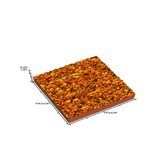
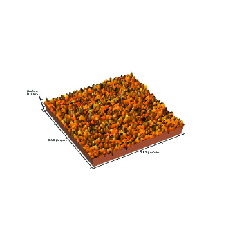
Figure 1: (Color online) Atomic force microscopy (AFM) surface images of two samples: (a) sample $1$ represents a surface with roughness $5.2nm$ and (b) sample $2$ represents a surface with roughness $3.6nm$.

II Statistical quantities

II.1 standard fractal analysis

For a sample of size $L$, roughness is defined by $w(L)=(\langle(h-\overline{h})^{2}\rangle)^{1/2}$ Barabasi , where $\langle\cdots\rangle$ denotes an spatial averaging samples, respectively. For simplicity, without losing the generality of the subject, we can assume that the mean height of the surface is zero, $\overline{h}=0$.

Roughness is one of the scaling properties of the surface. Roughness scales by size of the system as $w(L)\sim L^{\alpha}$, where $\alpha$ is the roughness exponent. The common procedure to measure the roughness exponent of a rough surface is based on a second moment of height difference function defined as $S^{2}(l)=\langle|h(x+l)-h(x)|^{2}\rangle$. This is equivalent to the statistics based on the height-height correlation function $C(l)=<h(x+l)h(x)>$ for stationary surfaces, i.e. $S^{2}(l)=2(w^{2}-C(l))$. The second order height difference function $S^{2}(l)$, scales with $l$ as $l^{\xi_{2}}$ where $\alpha=\xi_{2}/2$.

Assuming statistical translational invariance, different moments of the height difference functions $S^{q}(l)=<|h(x+l)-h(x)|^{q}>$, (qth moment of the increment of the rough surface height fluctuation $h(x)$) will depend only on the space difference of heights $l$, and has a power-law behavior if the process has the scaling property

$$S^{q}(l)=<|h(x+l)-h(x)|^{q}>\propto S^{q}(L_{0})\left({l\over\L_{0}}\right)^{\xi(q)},$$ (1)

where $L_{0}$ is the fixed largest length scale of the system, $<\cdot\cdot\cdot>$ denotes a statistical average (for non-overlapping increments of length $l$), $q$ is the order of the moment (we take here $q>0$), and $\xi_{q}$ is the exponent of the height difference function. The main property of a multifractal process is its characterization by a non-linear $\xi_{q}$ function of $q$. Monofractals are the generic result of the linear behavior. For instance, for Brownian motion (Bm) $\xi_{q}=q/2$, and for fractional Brownian motion (fBm) $\xi_{q}\propto q$.

II.2 Markov analysis

For better understanding the multifractality features, it can be useful to investigate the multifractality by Markov analysis. When long-range correlations are absent in $h(x)$, short-range correlations may exist. In this case, it can be more suitable to study multifractality by this approach. As a measure of surface roughness and to check the multifractal nature of rough surfaces, we check the Markovian nature of the increments which is defined by $h_{l}(x)=h(x+l)-h(x)$ depending on the length scale $l$.

First, we check whether $h_{l}(x)$ represents a Markov process Friedrich ; Waechter ; Jafari ; Peinke ; Shayeganfar ; Shayaganfar2. If so, we estimate the Markov Length scale (ML); the minimum length interval over which $h_{l}(x)$ can be represented by a Markov process. For a Markov process, knowledge of $P(h_{2},l_{2}|h_{1},l_{1})$ is sufficient for generating the entire statistics of $h_{l}(x)$, encoded in the n-point PDF that satisfies a master equation that, in turn, is reformulated by a Kramers-Moyal (KM) expansion,

$${\partial\over\partial l}p(h,l|h_{0},l_{0})=\sum_{k=1}^{\infty}\left(-{\partial\over\partial h}\right)^{k}[D_{k}(h,l)p(h,l|h_{0},l_{0})].$$ (2)

In order to obtain the drift ($D_{1}$) and diffusion coefficient ($D_{2}$)) for Eq. (2) we proceed in a well defined way like it was already expressed by Kolmogorov Friedrich1 ; Friedrich2 ; Waechter . The conditional moments $D_{k}(h,l)$ for finite step sizes $\Delta x$ are directly estimated from the data via moments of the conditional probabilities.

$$D_{k}(h,l)=\lim_{\Delta x\rightarrow 0}{l\over k!\Delta x}\int_{-\infty}^{\infty}(h^{\prime}-h)^{k}p(h^{\prime},l-\Delta x|h,l)d{h^{\prime}}.$$ (3)

For a general stochastic process, all the KM coefficients may be nonzero. However, provided that $D_{4}(h,l)$ vanishes or is small compared to the first two coefficients Risken , truncation of the KM expansion after the second term is meaningful in the statistical sense. For our samples, $D_{4}(h,l)$ is two orders of magnitude less than $D_{2}(h,l)$. Thus, we truncate the KM expansion after the second term, reducing it to a Fokker-Planck (FP) equation. According to the Ito calculus Risken , the FP equation is equivalent to a Langevin equation,

$${\partial\over\partial l}h(l)=D_{1}(h,l)+\sqrt{D_{2}(h,l)}f(l),$$ (4)

where $f(l)$ is a random force with zero mean and Gaussian statistics, $\delta$ -correlated in h, i.e., $<f(l)f(l^{\prime})>=2\delta(l-l^{\prime})$. $D_{1}$ is drift and $D_{2}$ is diffusion coefficients. To better clarify these variables ($D_{1}$ and $D_{2}$), we can pay attention to the Langvin equation (Eq. 4). Here, $D_{1}$ indicates an average height difference by walking on the surface ($\delta h=D_{1}\delta l$) and $D_{2}$ plays the role of the variance (uncertainty) of this height hanging ($f(l)D_{2}\delta l=\delta h$). To establish a relation between Markov approach and fractal distributions we start with the Fokker-Planck equation for PDF of the height increments

$$\Delta x{\partial\over\partial\Delta x}p(h,l)=[-{\partial\over\partial h}D_{1}(h,l)+{\partial^{2}\over\partial h^{2}}D_{2}(h,l)]p(h,l),$$ (5)

with the corresponding Langevin equation given by Eq. (4). It can be shown that for any series with the type of the correlations that is described by the self-affine distributions, the drift and diffusion coefficients of the increment series are given by Friedrich1 ; Friedrich2

$$D_{1}(h,l)\simeq-Hh$$

$$D_{2}(h,l)\simeq bh^{2}$$ (6)

where $H$ is the Hurst exponent which refers to the first moment exponent and $b$ indicates the strength of the multi-fractality. It means if $b=0$ in this case we find the samples mono-fractal. Thus, using Eqs. (5), we obtain the evolution of the moments of height difference function, $S_{q}(l)\equiv\langle|Deltah(l)|^{q}\rangle=\langle|h(x+l)-h(x)|^{q}\rangle$, as follows

$$-l{\partial\over\partial l}\langle|\Delta h(l)|^{q}\rangle=q\langle|\Delta h(l)|^{q-1}D_{1}(\Delta h,l)\rangle$$

$$+q(q-1)\langle|\Delta h(l)|^{q-2}D_{2}(\Delta h,l)\rangle$$ (7)

Then, by substituting Eq. (6) in Eq. (7) the scaling behavior of the moments of the height difference function are written as $S_{q}(l)\sim(l)^{\xi_{q}}$ then,

$$\xi_{q}=Hq-bq(q-1),$$ (8)

which establishes a direct link between the scaling exponents $\xi_{q}$ and the results obtained for the drift and diffusion coefficients.

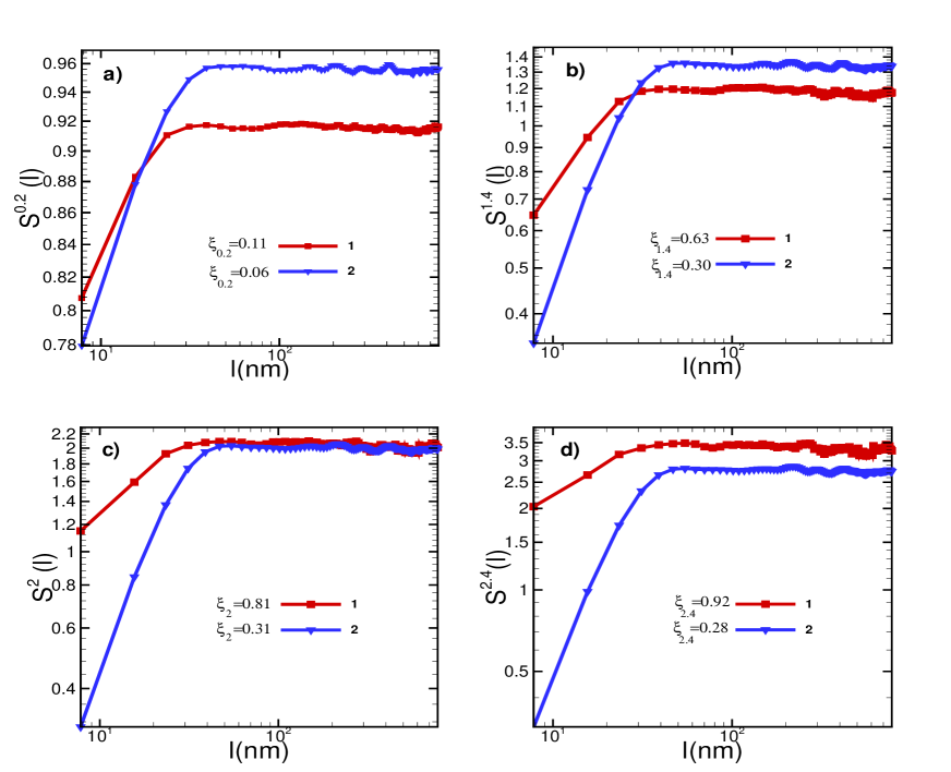
Figure 2: (Color online) Height difference functions of two samples (1 ($w=5.2nm$) and 2 ($w=3.6nm$)) for different moments q’s ((a) $q=0.2$, (b) $q=1.4$, (c) $q=2$ and (d) $q=2.4$), versus distance.

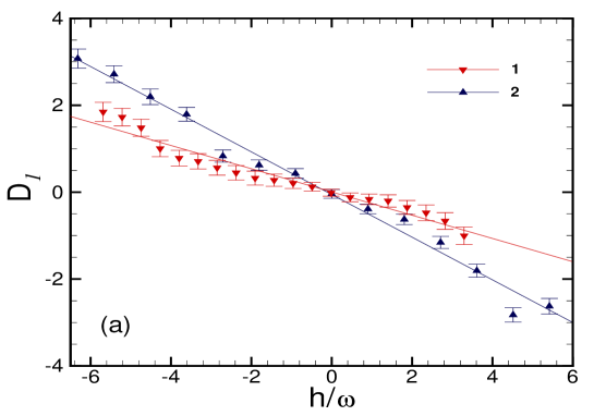
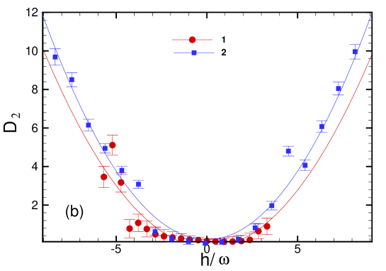
Figure 3: (Color online) Drift and diffusion coefficients of the two samples (1 ($w=5.2nm$) and 2 ($w=3.6nm$)) versus height which is normalized by roughness ($w$).

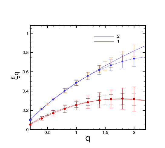
Figure 4: (Color online) Exponents of the qth moments of the height difference function of the two samples (1 ($w=5.2nm$) and 2 ($w=3.6nm$)) vs q. The errors from markovian methods are shown with the same color as the curves but the errors from the direct method are shown with different colors (black (sample 1) and orange (sample 2).

III Discussion and Results

In order to check the effect of coating rate on statistical properties of surfaces we have used samples of the same material (copper thin films) and equal thickness ($250nm$) which have been prepared in the same condition except their coating rates. We have chosen two of these samples ($1$ and $2$) typically for drawing the plots. In table I, experimental conditions of these selected thin layers are given. AFM method was used for obtaining microstructural data from the surfaces (Figs. 2a and 2b). Scaling properties were obtained using AFM images. In order to better explain the scaling properties of these surfaces, two points should be noted.

(a) Roughness is not an intrinsic property of the surface. Indeed, it depends on the scale of observation. In other words, when we observe a surface from various scales different roughness could be obtained.

(b) All information about the roughness is not included in the second moment of the height difference function mahsa2 . They used the concept of the higher moments to obtain further insights on roughness. They showed how these concepts could explain a rough surface for the purpose of suitable application and how experimental parameters can affect its properties.

Roughness of the two selected samples is different because of different coating rates. Normally, roughness is defined by root mean square of the height fluctuation (rms), however, roughness is not only determined from the second moment of the height fluctuation difference but also the other moments play role in the determination of the roughness which we call ”generalized roughness”. Fig. 2 (a-d) typically presents qth moment ($0.2,1.4,2$ and $2.4$) of the samples’ height fluctuation versus distance. Fig. 2 (c) presents second moment of the samples’ height difference function. The slope of each curve yields the roughness exponent of the corresponding surface. The scale of saturation limit in this curve is the correlation length. At scales larger than the correlation length the second moment saturates to a height $2w^{2}$. By increasing the order of moment, $q$, we see that the height of saturation of the moment is increased which is an indication of the generalized roughness. As it can be seen from the figure, after a particularhubi moment ($q>2$) the height difference function of the first sample lies above the second one which represents that the concept of roughness that is obtained from higher moments are larger for the sample $1$. In other words, higher moments focus on large height differences that occur in large scales. Thus, in large scales, sample $1$ is rougher than the second sample. It should be noted that the reported roughness in Tab. I presents the roughness for the largest scale which is the size of the system.

When we have fractal systems, their $\xi_{q}$ is a linear function of $q$ and this means that they are the same in their scaling behavior but for systems which are multifractal this behavior changes and the behavior of $\xi_{q}$ deviates from the simple linear relation with respect to $q$. As can be seen in Fig. 2, the scaling length, which is used to find the exponents $\xi_{q}$, is small. Thus, in order to find the behavior of the exponents of the height difference function moments we have used the Markov analysis too. In addition, this method helps us to better understand the multifractality of the surfaces under study. To use this approach we estimate the Markov Length scale (ML), the minimum length interval over which $h_{l}(x)$ can be represented by a Markov Process. To estimate the Markov length we have used Chapman Kolmogorov test. More detailed discussions of this test can be found in the appendix of Fazeli . The drift and diffusion coefficients, $D_{1}$ and $D_{2}$, were estimated directly from the data. They are well-represented by the approximates,

$$D_{1}(h,l)=\left\{\begin{array}[]{ll}-0.51\pm 0.01h,&\hbox{sample 1;}\\ -0.26\pm 0.03h,&\hbox{sample 2.}\end{array}\right.$$ (9)

and

$$D_{2}(h,l)=\left\{\begin{array}[]{ll}0.13\pm 0.01h^{2},&\hbox{sample 1;}\\ 0.10\pm 0.01h^{2},&\hbox{sample 2.}\end{array}\right.$$ (10)

Comparing Markov length scale and correlation length, ML is obtained directly from the joint PDF but the correlation length is obtained from height-height correlation function, which is the distance at which the correlation function falls to $1/e$ of its initial value. The Markov length scale of samples $1$ and $2$ are $1$ pixel ($7.8nm$) and $2$ pixel ($15.6nm$), respectively. Correlation length scale of samples $1$ and $2$ are $30nm$ and $47nm$, respectively. We summarized these quantities in Tab. I. For sample $2$, since its Markov length is other than one, we have considered the size effect for diffusion coefficient. The calculated diffusion coefficient for this sample is the one with the correction term. Non-negligible corrections have to be employed in order to get reliable estimates of diffusion coefficient for finite Markov length, $\Delta$ PRLkantz .

$$D_{2}(h,l,\Delta)=\frac{D_{2}(h,l)-(\Delta D_{1}(h,l))^{2}}{2\Delta(1+\Delta{D^{{}^{\prime}}_{1}}(h,l))}.$$ (11)

By obtaining the drift and diffusion coefficients (Fig. 3), the $\xi_{q}$ behavior from both standard fractal and Markov analysis has been calculated. Fig. 4 shows the results from both methods. The curves with error-bars are the ones calculated from the Markov analysis and the other two curves are from standard method. The equation for the $\xi_{q}$ for the two samples from the Markov analysis are $\xi(q)=(0.26\pm 0.03)q-0.10\pm 0.01q(q-1)$ for sample $1$ and $\xi(q)=(0.51\pm 0.01)q-0.13\pm 0.01q(q-1)$ for sample$2$.

As can be seen in Fig. 4, $\xi_{q}$ of both of our samples deviate from lines and the one which has larger root mean square (sample $1$) deviates more. Higher moments have more information from the larger fluctuations, which in correlated systems larger fluctuations appear in the larger scales. Here, $\xi_{q}$ of our samples shows how large scales play more effective role in the height fluctuation of sample $1$. This means that large moments of the rougher sample grow more with respect to the other sample. In other words, as can be seen in Fig. 2, in frame (a) the $q=0.2$ moment of height difference function of sample $1$ is below sample $2$ (after saturation length), but by increasing $q$ this behavior changes. Lower moments of sample $2$ are higher than sample $1$ and in the higher moments sample $1$ is higher. Lower moments describe the small height fluctuations in the surface.

To summarize, by increasing the coating rates, correlation length (grain sizes) and Markov length are decreased and roughness exponent is decreased and our surfaces become more multifractal.

Table 1: Experimental conditions and properties of the two selected copper thin layers: coating rate, coating time, thickness ($\tau$), Roughness ($w$), pixel’s size, correlation length ($l_{cor}$), roughness exponent ($\alpha$) and Markov length scale.

Sample	Coating rate ($\frac{nm}{sec}$)	$t(sec)$	$\tau(nm)$	$w(nm)$	Pixel’s size ($nm$)	$l_{cor}$ ($nm$)	$\alpha$	ML ($nm$)
$1$	1.9 $\pm$ 0.04	128 $\pm$ 1	250 $\pm$ 5	5.2 $\pm$ 0.2	7.8	31 $\pm$ 7.8	0.20 $\pm$ 0.01	7.8
$2$	1.7 $\pm$ 0.04	145 $\pm$ 1	250 $\pm$ 5	3.6 $\pm$ 0.2	7.8	47 $\pm$ 7.8	0.40 $\pm$ 0.01	15.6

IV Conclusion

Different conditions in particle deposition leads to the change in the topography of the surfaces. We have shown that by changing the coating rate properties of the surface differ. The average energy of the depositing particles is increased by raising the coating rate. In this case, the particles penetrate through the surface and this affects the roughness and multifractality of the surface.

References

- (1) M. Paillet, P. Poncharal, and A. Zahab, Phys. Rev. Lett. 94, 186801 (2005).
- (2) Y. Yaish, J.-Y. Park, S. Rosenblatt, V. Sazonova, M. Brink, P. L. McEuen, Phys. Rev. Lett. 92, 046401 (2004).
- (3) G. R. Jafari, S. M. Mahdavi, A. Iraji zad and P. Kaghazchi, Surface and Interface Analysis 37, 641 (2005).
- (4) B. N. J. Persson, O. Albohr, U. Tartaglino, A. I. Volokitin and E. Tosatti, J. Phys. Condens. Matter 17, R1 R62 (2005).
- (5) A. G. Peressadko, N. Hosoda, and B. N. J. Persson, Phys. Rev. Lett. 95, 124301 (2005).
- (6) B. N. J. Persson, J. Chem. Phys. 115, 3840 (2001).
- (7) J. A. Ogilvy, Theory of Wave Scattering from Random Rough Surfaces (Bristol: Institute of Physics Publishing 1991); A. G. Voronovich, Wave Scattering from Rough Surfaces 2nd updated edn (Heidelberg: Springer 1994).
- (8) A. V. Karabutov, V. D. Frolov, E. N. Loubnin, A. V. Simakin, G. A. Shafeev, Appl. Phys. A 76, 413 (2003).
- (9) M. Suchea, S. Christoulakis, K. Moschovis, N. Katsarakis, G. Kiriakidis, Thin Solid Films 515, 551 (2006).
- (10) J. Bico, C. Marzolin and D. Quere, Europhys. Lett. 47, 220 (1999).
- (11) A. L. Barabasi and H. E. Stanley, Fractal Concepts in Surface Growth (Cambridge University Press, New York, 1995); P. Meakin Fractals, Scaling and Growth Far From Equilibrium (Cambridge University Press, Cambridge, 1998).
- (12) M. Vahabi, G. R. Jafari, N. Mansour, R. Karimzadeh, J. Zamiranvari, J. Stat. Mech. P03002 (2008).
- (13) R. Friedrich and J. Peinke, Phys. Rev. Lett. 78, 863 (1997).
- (14) S. M. Fazeli, A. H. Shirazi and G. R. Jafari, New Journal of Physics 10, 083020 (2008).
- (15) G. R. Jafari, S. M. Fazeli, F. Ghasemi, S. M. Vaez Allaei, M. Reza Rahimi Tabar, A. Iraji zad, and G. Kavei, Phys. Rev. Lett. 91, 226101 (2003).
- (16) F. Ghasemi, M. Sahimi, J. Peinke, R. Friedrich, G. R. Jafari, and M. R. Rahimi Tabar, Phys. Rev. E 75, 060102(R) (2007).
- (17) F. Shayeganfar, S. Jabbari-Farouji, M. Sadegh Movahed, G. R. Jafari, and M. Reza Rahimi Tabar, Phys. Rev. E 80, 061126 (2009).
- (18) F. Shayeganfar, S. Jabbari-Farouji, M. Sadegh Movahed, G. Reza Jafari, M. Reza Rahimi Tabar, Phys. Rev. E 81, 061404 (2010).
- (19) H. Risken, The Fokker-Planck Equation, 2nd ed. (Springer, Berlin, 1989).
- (20) R. Friedrich, J. Peinke, and Ch. Renner, Phys. Rev. Lett 84, 5224 (2000).
- (21) Ch. Renner, J. Peinke, and R. Friedrich, J. Fluid. Mech. 433, 383 (2001).
- (22) M. Waechter, F. Riess, Th. Schimmel, U. Wendt, and J. Peinke, Eur. Phys. J. B 41, 259 (2004).
- (23) Mario Ragwitz and Holger Kantz, Phys. Rev. Lett 87, 254501 (2001).