Time-dependent localized Hartree-Fock potential

Abstract

By minimizing the difference between the left- and the right-hand sides of the many-body time-dependent Schrödinger equation with the Slater-determinant wave-function, we derive a non-adiabatic and self-interaction free time-dependent single-particle effective potential which is the generalization to the time-dependent case of the localized Hartree-Fock potential. The new potential can be efficiently used within the framework of the time-dependent density-functional theory as we demonstrate by the evaluation of the wave-vector and frequency dependent exchange kernel $f_{x}(q,\omega)$ and the exchange shear modulus $\mu_{x}$ of the homogeneous electron gas.

Time-dependent (TD) density-functional theory (DFT) Zangwill and Soven (1980); *Runge-84; *Gross-85 is in the perpetual search of effective single-particle potentials which accurately (in ideal - exactly) map the propagation of an interacting many-body system onto that of the non-interacting one. While the exchange-correlation (xc) functionals based on the Local-Density Approximation (LDA) Kohn and Sham (1965); Perdew and Wang (1992) and its semi-local refinement of the Generalized Gradient Approximation (GGA) Perdew and Yue (1986); Perdew et al. (1996a, b); *Perdew-96-e have proven very successful in the ground-state DFT, in TDDFT the usefulness of (semi-) local approaches is limited due to the fundamental spatial non-locality of the exact time-dependent xc functional Vignale (1995).

Beyond LDA and GGA, the concept of the optimized effective potential (OEP) Sharp and Horton (1953); Talman and Shadwick (1976) plays one of the key roles in the systematic non-heuristic construction of DFT. In the ground-state case, OEP is defined as a single-particle potential which minimizes the many-body Hamiltonian expectation value on the Slater-determinant wave-function. From the DFT perspective, OEP is the first term in the adiabatic connection series in the powers of the interaction constant (exact exchange) Görling and Levy (1994). The generalization of the OEP to the time-dependent case has been proposed Ullrich et al. (1995), which, however, is impractical for applications due to the formidable complexity of the integral equation involved.

In this work we propose and implement an alternative approach to the development of the time-dependent single-particle effective potential for many-body problems. This is based on the variational principle of the minimization of the difference between the left- and right-hand sides of the time-dependent Schrödinger equation, which principle we had introduced almost three decades ago Nazarov (1985). By this and with no further approximations or ad hoc assumptions, we derive a time-dependent effective potential with the following useful properties: (i) It satisfies the exact large-separation asymptotic condition and is self-interaction free; (ii) It is expressed in terms of an equation easily solvable for both a finite and an infinite periodic (or homogeneous) problems; (iii) In the static case, our effective potential reduces to the earlier known localized Hartree-Fock (HF) potential Della Sala and Gorling (2001). As an immediate application of this approach, we derive the dynamic exchange kernel $f_{x}(q,\omega)$ and the exchange shear modulus $\mu_{x}$ Qian and Vignale (2002) of the homogeneous electron gas (HEG).

Let us consider a $N$-electrons system with the Hamiltonian

$$\hat{H}(t)=\sum\limits_{i}\left[-\frac{1}{2}\Delta_{i}+v_{ext}(\mathbf{r}_{i},t)\right]+\sum\limits_{i<j}\frac{1}{|\mathbf{r}_{i}-\mathbf{r}_{j}|}.$$ (1)

The many-body wave-function $\Psi(t)$ satisfies the Schrödinger equation

$$i\dot{\Psi}(t)=\hat{H}(t)\Psi(t),$$

where the dot denotes the time derivative. We are asking the question: What is the potential $v_{eff}(\mathbf{r},t)$ such that the functional

$$\int\left|i\dot{\Psi}_{s}(t)-\hat{H}(t)\Psi_{s}(t)\right|^{2}d\mathbf{r}_{1}...d\mathbf{r}_{N}$$ (2)

is minimal at an arbitrary time $t$ for the wave-function $\Psi_{s}(t)$ being the Slater determinant built with the single-particle orbitals $\psi_{\alpha}(\mathbf{r},t)$ which satisfy the single-particle Schrödinger equation

$$i\dot{\psi}_{\alpha}(\mathbf{r},t)=\left[-\frac{1}{2}\Delta+v_{eff}(\mathbf{r},t)\right]\psi_{\alpha}(\mathbf{r},t).$$ (3)

Let us assume that the TD part of $v_{ext}(\mathbf{r},t)$ was absent at $t<0$, and we have already solved the static problem of determining $v_{eff}(\mathbf{r})$ at $t<0$ and the corresponding orbitals $\psi_{\alpha}(\mathbf{r},t)$ at $t\leq 0$. At $t=0$, the time-dependence of the potential is switched on. Knowing the orbitals $\psi_{\alpha}(\mathbf{r},0)$, we find $v_{eff}(\mathbf{r},0)$ which, determining $\dot{\psi}_{\alpha}(\mathbf{r},0)$ by Eq. (3), minimizes the functional (2) at $t=0$. We then find $\psi_{\alpha}(\mathbf{r},\Delta t)\approx\psi_{\alpha}(\mathbf{r},0)+\dot{\psi}_{\alpha}(\mathbf{r},0)\Delta t$, where $\Delta t$ is a small time increase. The procedure is repeated up to an arbitrary time $t$.

In the $\Delta t\rightarrow 0$ limit, this scheme reads: With fixed (but yet unknown) orbitals $\psi_{\alpha}(\mathbf{r},t)$, we are looking for the potential $v_{eff}(\mathbf{r},t)$ which, determining $\dot{\psi}_{\alpha}(\mathbf{r},t)$ by Eq. (3), minimizes the functional (2). This gives $v_{eff}(\mathbf{r},t)$ as a functional of the orbitals, and, finally, the orbitals themselves are found by the self-consistent solution of Eqs. (3). We note that a procedure of the minimization of the same functional (2) with respect to $\dot{\psi}_{\alpha}$ as independently varied functions retrieves the TD HF equations Nazarov (1985).

Since $\Psi_{s}(t)$ obviously satisfies the equation

$$i\dot{\Psi}_{s}(t)=\sum\limits_{i}\left[-\frac{1}{2}\Delta_{i}+v_{eff}(\mathbf{r}_{i},t)\right]\Psi_{s}(t),$$ (4)

the functional (2) can be rewritten as

$$\int\left[\sum\limits_{i}\tilde{v}(\mathbf{r}_{i},t)-\sum\limits_{i<j}\frac{1}{|\mathbf{r}_{i}-\mathbf{r}_{j}|}\right]^{2}\left|\Psi_{s}(t)\right|^{2}d\mathbf{r}_{1}...d\mathbf{r}_{N},$$ (5)

where $\tilde{v}=v_{eff}-v_{ext}$. Equating to zero the first variation of Eq. (5) with respect to $\delta\tilde{v}=\delta v$, we find

$$\begin{split}\int\left[\sum\limits_{i}\tilde{v}(\mathbf{r}_{i},t)-\sum\limits_{i<j}\frac{1}{|\mathbf{r}_{i}-\mathbf{r}_{j}|}\right]\left|\Psi_{s}(t)\right|^{2}\\ \times\sum\limits_{i}\delta\tilde{v}(\mathbf{r}_{i},t)d\mathbf{r}_{1}...d\mathbf{r}_{N}=0,\end{split}$$ (6)

which can be rewritten using the permutational symmetry of the wave-function as

$$\!\int\!\left[\sum\limits_{i}\tilde{v}(\mathbf{r}_{i},t)\!-\!\sum\limits_{i<j}\frac{1}{|\mathbf{r}_{i}\!-\!\mathbf{r}_{j}|}\right]\left|\Psi_{s}(t)\right|^{2}\delta\tilde{v}(\mathbf{r}_{1},t)d\mathbf{r}_{1}...d\mathbf{r}_{N}\!=\!0,$$

and, due to the arbitrariness of $\delta\tilde{v}$,

$$\int\left[\sum\limits_{i}\tilde{v}(\mathbf{r}_{i},t)-\sum\limits_{i<j}\frac{1}{|\mathbf{r}_{i}-\mathbf{r}_{j}|}\right]\left|\Psi_{s}(t)\right|^{2}d\mathbf{r}_{2}...d\mathbf{r}_{N}=0.$$ (7)

Straightforward but rather lengthy transformations carried out in Ref.  lead from Eq. (7) to the following equation for the exchange potential $v_{x}=\tilde{v}-v_{H}$, where $v_{H}(\mathbf{r})$ is the Hartree potential,

$$\begin{split}n(\mathbf{r},t)v_{x}(\mathbf{r},t)=\int\left[v_{x}(\mathbf{r}_{1},t)\!-\!\frac{1}{|\mathbf{r}-\mathbf{r}_{1}|}\right]|\rho(\mathbf{r},\mathbf{r}_{1},t)|^{2}d\mathbf{r}_{1}\\ +\int\frac{\rho(\mathbf{r},\mathbf{r}_{1},t)\rho(\mathbf{r}_{1},\mathbf{r}_{2},t)\rho(\mathbf{r}_{2},\mathbf{r},t)}{|\mathbf{r}_{1}-\mathbf{r}_{2}|}d\mathbf{r}_{1}d\mathbf{r}_{2},\end{split}$$ (8)

where

$$n(\mathbf{r},t)=\sum\limits_{\alpha=1}^{N}|\psi_{\alpha}(\mathbf{r},t)|^{2},$$ (9)

$$\rho(\mathbf{r},\mathbf{r}_{1},t)=\sum\limits_{\alpha=1}^{N}\psi_{\alpha}(\mathbf{r},t)\psi_{\alpha}^{*}(\mathbf{r}_{1},t)$$ (10)

are the particle density and the single-particle density-matrix, respectively . Equation (8) is our main result. We note that the only difference of Eq. (8) from the earlier known equation for the static localized HF potential (see Refs. Della Sala and Gorling, 2001 and Zhou and Chu, 2005 for spin-neutral and spin-polarized cases, respectively) is the time-dependence of all the quantities involved. It must, however, be emphasized that without the derivation from the time-dependent variational principle, the generalization of the static localized HF potential to the time-dependent case by just inserting the time variable into the static equation would have been ungrounded. Trivially, Eq. (8) reduces to the equation for the localized HF potential in the time-independent case.

Solution of Eq. (8) in the case of a few-body system does not present a difficult problem, as have already been pointed out in Ref. Della Sala and Gorling, 2001 in conjunction with the time-independent case: Due to Eq. (10), the kernel $|\rho(\mathbf{r},\mathbf{r}_{1},t)|^{2}$ of the integral equation (8) is a separable function with respect to $\mathbf{r}$ and $\mathbf{r}^{\prime}$ variables. Neither presents it a problem in the case of infinite periodic systems, when the equation reduces to the matrix one. We now apply the TD localized HF potential to obtain the wave-vector and frequency dependent exchange kernel $f_{x}(q,\omega)$ of HEG, which, being a fundamental quantity by itself, is also an important input in the theory of optical response of a weakly ingomogeneous interacting electron gas Nazarov et al. (2009).

Dynamic exchange kernel of HEG – In the case of HEG and a weak externally applied potential $\delta v_{ext}(\mathbf{r},t)=\delta v_{ext}(\mathbf{q},\omega)e^{i(\mathbf{q}\cdot\mathbf{r}-\omega t)}$, we linearize Eq. (8) with respect to the latter potential. The zero-order orbitals are plane-waves , and to the zeroth and first orders we have for the density-matrix

$$\begin{split}&\rho_{0}(\mathbf{r},\mathbf{r}_{1})=\frac{2}{V}\sum\limits_{\mathbf{k}}\int f(\epsilon_{\mathbf{k}})e^{i\mathbf{k}\cdot(\mathbf{r}-\mathbf{r}_{1})},\\ &\delta\rho(\mathbf{r},\mathbf{r}_{1},\omega)\!=\!\delta v_{s}(\mathbf{q},\omega)\,e^{i\mathbf{q}\cdot\mathbf{r}}\frac{2}{V}\!\sum\limits_{\mathbf{k}}\!\frac{f(\epsilon_{\mathbf{k}})\!-\!f(\epsilon_{\mathbf{k}+\mathbf{q}})}{\omega\!-\!\epsilon_{\mathbf{k}+\mathbf{q}}\!+\!\epsilon_{\mathbf{k}}\!+\!i\eta}e^{i\mathbf{k}\cdot(\mathbf{r}\!-\!\mathbf{r}_{1})},\end{split}$$ (11)

where $\epsilon_{\mathbf{k}}=k^{2}/2$ are free-particle eigenenergies, $f(\epsilon_{\mathbf{k}})$ are their occupation numbers, $\delta v_{s}(\mathbf{q},\omega)$ is the perturbation of the Kohn-Sham (KS) potential, $V$ is the normalization volume, and $\eta$ is an infinitesimal positive. After linearization, Eq. (8) yields

$$\begin{split}\frac{\delta v_{x}(q,\omega)}{\delta v_{s}(q,\omega)}=\frac{4\pi}{(2\pi)^{3}}\int\left[\frac{1}{\omega\!-\!\epsilon_{\mathbf{k}+\mathbf{q}}\!+\!\epsilon_{\mathbf{k}}\!+\!i\eta}-\frac{1}{\omega\!+\!\epsilon_{\mathbf{k}+\mathbf{q}}\!-\!\epsilon_{\mathbf{k}}\!+\!i\eta}\right]\frac{f(\epsilon_{\mathbf{k}})B(\mathbf{q},\mathbf{k})-f(\epsilon_{\mathbf{k}+\mathbf{q}})[f(\epsilon_{\mathbf{k}})-1]C(k)}{n_{0}-A(q)}d\mathbf{k},\end{split}$$ (12)

where

$$A(q)=\frac{2}{(2\pi)^{3}}\int f(\epsilon_{\mathbf{k}})f(\epsilon_{\mathbf{k}+\mathbf{q}})d\mathbf{k},$$ (13)

$$B(\mathbf{q},\mathbf{k})=\frac{2}{(2\pi)^{3}}\int\frac{f(\epsilon_{\mathbf{k}_{1}})f(\epsilon_{\mathbf{k}_{1}+\mathbf{q}})}{|\mathbf{k}-\mathbf{k}_{1}|^{2}}d\mathbf{k}_{1},$$ (14)

$$C(k)=\frac{2}{(2\pi)^{3}}\int\frac{f(\epsilon_{\mathbf{k}_{1}})}{|\mathbf{k}-\mathbf{k}_{1}|^{2}}d\mathbf{k}_{1}.$$ (15)

With the use of Eq. (12), the exchange kernel is now found as

$$\begin{split}&f^{h}_{x}(q,\omega)\equiv\frac{\delta v_{x}(q,\omega)}{\delta n(q,\omega)}=\\ &\frac{\delta v_{x}(q,\omega)}{\delta v_{s}(q,\omega)}\frac{\delta v_{s}(q,\omega)}{\delta n(q,\omega)}=\frac{\delta v_{x}(q,\omega)}{\delta v_{s}(q,\omega)}\left(\chi_{s}^{h}\right)^{-1}(q,\omega),\end{split}$$ (16)

where $\chi^{h}_{s}(q,\omega)$ is Lindhard density-response function Lindhard (1954)

$$\chi^{h}_{s}(q,\omega)=\frac{2}{V}\sum\limits_{\mathbf{k}}\frac{f(\epsilon_{\mathbf{k}})\!-\!f(\epsilon_{\mathbf{k}+\mathbf{q}})}{\omega\!-\!\epsilon_{\mathbf{k}+\mathbf{q}}\!+\!\epsilon_{\mathbf{k}}\!+\!i\eta}.$$ (17)

In Ref. , we evaluate integrals (13) and (15) analytically and reduce the integral (14) to a single-fold one.

It can be seen from Eqs. (12) and (16) that ${\rm Im}\,f_{x}$ is nonzero inside the single particle-hole excitation continuum only. This deficiency of $f_{x}$ derived from TD localized HF potential is not limited to HEG, but, as can be easily seen, persists for any extended (periodic) system. Therefore, such subtle effect as the high-frequency tail of ${\rm Im}\,f_{x}$ of HEG Sturm and Gusarov (2000) cannot be accounted for within the present approach. Instead, we will now show that $f_{x}$ derived from the TD localized HF potential significantly corrects the Lindhard dielectric function of HEG within the single particle-hole continuum.

In Fig. 1, the exchange kernel $f^{h}_{x}(q,\omega)$ obtained by the use of Eqs. (12) and (16) is plotted at $q=0.5\times k_{F}$ for $r_{s}=2$ and $5$. With the inclusion of $f_{x}$, the dielectric function of HEG can be written as

$$\epsilon^{h}(q,\omega)=1-\frac{4\pi}{q^{2}}\frac{\chi^{h}_{s}(q,\omega)}{1+\chi^{h}_{s}(q,\omega)f^{h}_{x}(q,\omega)}.$$ (18)

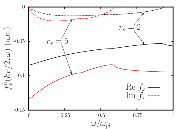
Figure 1: (color online) Exchange kernel $f^{h}_{x}(q,\omega)$, $q=0.5\times k_{F}$, of HEG of $r_{s}=2$ (black curves online) and $r_{s}=5$ (red curves online). Solid and dashed curves are real and imaginary parts of $f^{h}_{x}$.

In Fig. 2, the dielectric function of HEG of $r_{s}=5$ obtained through Eq. (18) is plotted together with the Lindhard dielectric function. From this we judge that dynamic exchange plays a significant role at this density and can hardly be considered as a weak perturbation.

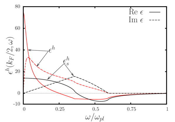
Figure 2: (color online) Dielectric function $\epsilon^{h}(q,\omega)$, $q=0.5\times k_{F}$, of HEG of $r_{s}=5$ evaluated by the use of EQ. (18) with the exchange kernel $f^{h}_{x}$ included (red curves online) and its Lindhard counterpart $\epsilon^{h}_{s}(q,\omega)$ (black curves online). Solid and dashed curves are real and imaginary parts of the dielectric function, respectively.

In Fig. 3, the static exchange kernel $f^{h}_{x}(q)$ is plotted for HEG of $r_{s}=5$ as a function of the wave-vector. We find a qualitative agreement with the Monte Carlo (MC) simulations of Ref. Moroni et al., 1995.

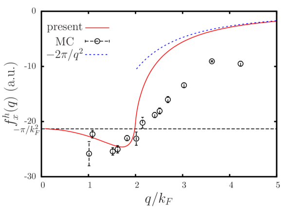
Figure 3: (color online) Static exchange kernel $f^{h}_{x}(q)$ of HEG of $r_{s}=5$. Solid line (red online) is the present result. Symbols with error bars are $f^{h}_{xc}(q)$ by MC simulations from Ref. Moroni et al. (1995). The dashed line (blue online) shows the asymptotic behavior at large $q$, as stipulated by Eq. (21).

The following limiting cases can be further worked out from Eqs. (12)-(15)

$$\lim_{q\rightarrow 0}f_{x}^{h}(q,\omega\neq 0)=-\frac{3\pi}{4k_{F}^{2}},$$ (19)

$$\lim_{q\rightarrow 0}\lim_{\omega\rightarrow 0}f_{x}^{h}(q,\omega)=-\frac{\pi}{k_{F}^{2}},$$ (20)

$$\lim_{q\rightarrow\infty}\lim_{\omega\rightarrow 0}f_{x}^{h}(q,\omega)=-\frac{2\pi}{q^{2}},$$ (21)

and since Qian and Vignale (2002)

$$\left[\lim_{\omega\rightarrow 0}\lim_{q\rightarrow 0}-\lim_{q\rightarrow 0}\lim_{\omega\rightarrow 0}\right]f_{x}^{h}(q,\omega)=\frac{4}{3}\frac{\mu_{xc}}{n^{2}},$$ (22)

where $\mu_{x}$ is the exchange contribution to the shear modulus of HEG, we can write by virtue of Eqs. (19), (20), and (22)

$$\mu_{x}=\frac{3\left(\frac{3}{2}\right)^{2/3}}{64\pi^{5/3}r_{s}^{4}}\approx\frac{0.0091}{r_{s}^{4}},$$ (23)

which is smaller than the high-density result of Ref. Conti and Vignale, 1999: $\mu_{xc}=\frac{3\left(\frac{3}{2}\right)^{2/3}}{40\pi^{5/3}r_{s}^{4}}\approx\frac{0,0146}{r_{s}^{4}}$. In Table 1, we compare $\mu_{x}$ obtained via Eq. (23) with $\mu_{xc}$ of Refs. Qian and Vignale, 2002, Böhm et al., 1996; *Conti-97; *Nifosi-97; *Nifosi-98, and Conti and Vignale, 1999.

Table 1: Exchange shear modulus $\mu_{x}$ in units of $2\omega_{pl}n$. Present results are shown together with those for $\mu_{xc}$ of Refs. Qian and Vignale, 2002 (QV), Böhm et al., 1996; *Conti-97; *Nifosi-97; *Nifosi-98 (NCT), and Conti and Vignale, 1999 (CV).

$r_{s}$	1	2	3	4	5
present	0.01102	0.01559	0.01909	0.02204	0.02464
QV	0.00738	0.00770	0.00801	0.00837	0.00851
NCT	0.0064	0.052	0.0037	0.0020	0.0002
CV	0.01763	0.02494	0.03054	0.03527	0.03943

In conclusion, within the well-defined procedure of the minimization of the difference between the left- and right-hand sides of the time-dependent Shrödinger equation, we have derived a time-dependent single-particle effective potential for a system of arbitrary number of electrons under the action of a time-dependent external field. This potential is non-local, non-adiabatic, and self-interaction free, and it satisfies the exact large-separation asymptotic condition. At the same time, our effective potential is comparatively easy for evaluation, which is in contrast to earlier known TD optimized effective potential. These properties open a way to efficiently use this potential within the context of time-dependent density-functional theory, as we demonstrate by the derivation of the exchange kernel $f_{x}(q,\omega)$ of the homogeneous electron gas.

I SUPPLEMENTAL MATERIAL
 
to the paper by V. U. Nazarov
 
“Time-dependent localized Hartree-Fock potential”

I.1 Derivation of Eq. (8).

Using the permutational symmetry, we can rewrite Eq. (7) as

$$\tilde{v}(\mathbf{r}_{1},t)\int\left|\Psi_{s}(t)\right|^{2}d\mathbf{r}_{2}...d\mathbf{r}_{N}+\int\left[(N-1)\tilde{v}(\mathbf{r}_{2},t)-\frac{(N-1)}{|\mathbf{r}_{1}-\mathbf{r}_{2}|}-\frac{(N-1)(N-2)}{2|\mathbf{r}_{2}-\mathbf{r}_{3}|}\right]\left|\Psi_{s}(t)\right|^{2}d\mathbf{r}_{2}...d\mathbf{r}_{N}=0,$$ (S.1)

or

$$\frac{\tilde{v}(\mathbf{r}_{1},t)n(\mathbf{r}_{1},t)}{N}+(N-1)\int\left[\tilde{v}(\mathbf{r}_{2},t)-\frac{1}{|\mathbf{r}_{1}-\mathbf{r}_{2}|}-\frac{N-2}{2|\mathbf{r}_{2}-\mathbf{r}_{3}|}\right]\left|\Psi_{s}(t)\right|^{2}d\mathbf{r}_{2}...d\mathbf{r}_{N}=0,$$ (S.2)

where $n(\mathbf{r},t)$ is the particle-density. Further simplifications give

$$\frac{\tilde{v}(\mathbf{r}_{1},t)}{N(N-1)}\!+\!\int\!\left[\tilde{v}(\mathbf{r}_{2},t)\!-\!\frac{1}{|\mathbf{r}_{1}-\mathbf{r}_{2}|}\right]\frac{\rho_{2}(\mathbf{r}_{1},\mathbf{r}_{2};\mathbf{r}_{1},\mathbf{r}_{2};t)}{n(\mathbf{r}_{1},t)}d\mathbf{r}_{2}-\frac{(N\!-\!2)}{2}\!\int\!\frac{\rho_{3}(\mathbf{r}_{1},\mathbf{r}_{2},\mathbf{r}_{3};\mathbf{r}_{1},\mathbf{r}_{2},\mathbf{r}_{3};t)}{n(\mathbf{r}_{1},t)|\mathbf{r}_{2}-\mathbf{r}_{3}|}d\mathbf{r}_{2}d\mathbf{r}_{3}\!=\!0,$$ (S.3)

where the $k$-particle density-matrix is

$$\rho_{k}(\mathbf{r}_{1},...\mathbf{r}_{k};\mathbf{r}_{1}^{\prime},...\mathbf{r}_{k}^{\prime};t)=\int\Psi_{s}(\mathbf{r}_{1}...\mathbf{r}_{k},\mathbf{r}_{k+1}^{\prime\prime}...\mathbf{r}_{N}^{\prime\prime},t)\Psi_{s}^{*}(\mathbf{r}_{1}^{\prime}...\mathbf{r}_{k}^{\prime},\mathbf{r}_{k+1}^{\prime\prime}...\mathbf{r}_{N}^{\prime\prime},t)d\mathbf{r}_{k+1}^{\prime\prime}...d\mathbf{r}_{N}^{\prime\prime}.$$ (S.4)

For the Slater determinant wave-function $\Psi_{s}(t)$ the equalities hold

$$\rho_{2}(\mathbf{r}_{1},\mathbf{r}_{2};\mathbf{r}_{1},\mathbf{r}_{2};t)=\frac{1}{N(N\!-1\!)}\left[n(\mathbf{r}_{1},t)n(\mathbf{r}_{2},t)-|\rho(\mathbf{r}_{1};\mathbf{r}_{2},t)|^{2}\right],$$ (S.5)

$$\begin{split}&\rho_{3}(\mathbf{r}_{1},\mathbf{r}_{2},\mathbf{r}_{3};\mathbf{r}_{1},\mathbf{r}_{2},\mathbf{r}_{3};t)=\frac{1}{N(N\!-1\!)(N\!-\!2)}\left[n(\mathbf{r}_{1},t)n(\mathbf{r}_{2},t)n(\mathbf{r}_{3},t)-n(\mathbf{r}_{2},t)|\rho(\mathbf{r}_{1};\mathbf{r}_{3},t)|^{2}\right.-n(\mathbf{r}_{3},t)|\rho(\mathbf{r}_{1};\mathbf{r}_{2},t)|^{2}\\ &-n(\mathbf{r}_{1},t)|\rho(\mathbf{r}_{2};\mathbf{r}_{3},t)|^{2}+\rho(\mathbf{r}_{1};\mathbf{r}_{2},t)\rho(\mathbf{r}_{2};\mathbf{r}_{3},t)\rho(\mathbf{r}_{3};\mathbf{r}_{1},t)\left.+\rho(\mathbf{r}_{1};\mathbf{r}_{3},t)\rho(\mathbf{r}_{3};\mathbf{r}_{2},t)\rho(\mathbf{r}_{2};\mathbf{r}_{1},t)\right],\end{split}$$ (S.6)

where

$$\rho(\mathbf{r};\mathbf{r}^{\prime},t)=N\rho_{1}(\mathbf{r};\mathbf{r}^{\prime},t)=\sum\limits_{\alpha}\psi_{\alpha}(\mathbf{r},t)\psi_{\alpha}^{*}(\mathbf{r}^{\prime},t).$$ (S.7)

Therefore

$$\begin{split}\tilde{v}(\mathbf{r}_{1},t)-V_{H}(\mathbf{r}_{1},t)\!-\!\int\!\left[\tilde{v}(\mathbf{r}_{2},t)\!-\!\frac{1}{|\mathbf{r}_{1}-\mathbf{r}_{2}|}\right]\frac{|\rho(\mathbf{r}_{1};\mathbf{r}_{2};t)|^{2}}{n(\mathbf{r}_{1},t)}d\mathbf{r}_{2}+\!\int\!\frac{n(\mathbf{r}_{2},t)|\rho(\mathbf{r}_{1};\mathbf{r}_{3},t)|^{2}}{n(\mathbf{r}_{1},t)|\mathbf{r}_{2}-\mathbf{r}_{3}|}d\mathbf{r}_{2}d\mathbf{r}_{3}\\ -\!\int\!\frac{\rho(\mathbf{r}_{1};\mathbf{r}_{2},t)\rho(\mathbf{r}_{2};\mathbf{r}_{3},t)\rho(\mathbf{r}_{3};\mathbf{r}_{1},t)}{n(\mathbf{r}_{1},t)|\mathbf{r}_{2}-\mathbf{r}_{3}|}d\mathbf{r}_{2}d\mathbf{r}_{3}+C(t)\!=\!0,\ \end{split}$$ (S.8)

where

$$V_{H}(\mathbf{r},t)=\int\frac{n(\mathbf{r}^{\prime},t)}{|\mathbf{r}-\mathbf{r}^{\prime}|}d\mathbf{r}^{\prime},$$ (S.9)

$$C(t)=\int\tilde{v}(\mathbf{r}_{2},t)n(\mathbf{r}_{2},t)d\mathbf{r}_{2}-\frac{1}{2}\!\int\!\frac{n(\mathbf{r}_{2},t)n(\mathbf{r}_{3},t)}{|\mathbf{r}_{2}-\mathbf{r}_{3}|}d\mathbf{r}_{2}d\mathbf{r}_{3}+\frac{1}{2}\!\int\!\frac{|\rho(\mathbf{r}_{2};\mathbf{r}_{3},t)|^{2}}{|\mathbf{r}_{2}-\mathbf{r}_{3}|}d\mathbf{r}_{2}d\mathbf{r}_{3}=0,$$ (S.10)

and the second equality in Eq. (S.10) follows from Eq. (S.8). Eqs. (S.8) and (S.10) give immediately Eq. (8).

I.2 Integrals (13)-(15).

For integrals (13) and (15) we have straightforwardly

$$A(q)=\frac{1}{48\pi^{2}}\Theta(2k_{F}-q)(2k_{F}-q)^{2}(4k_{F}+q),$$ (S.11)

$$C(k)=\frac{2}{(2\pi)^{3}}H(k,k_{F}),$$ (S.12)

where $\Theta(x)$ is the Heaviside’s step function and

$$H(k,p)=\frac{\pi}{k}\left[(p^{2}-k^{2})\log\left|\frac{p+k}{p-k}\right|+2kp\right].$$ (S.13)

For integral (14) we have

$$B(\mathbf{q},\mathbf{k})=\frac{2}{(2\pi)^{3}}\Theta(k_{F}-q)H(k,k_{F}-q)+\frac{2}{(2\pi)^{2}}\Theta(2k_{F}-q)\int\limits_{|k_{F}-q|}^{k_{F}}P\left(k,k_{1},\frac{k_{F}^{2}-k_{1}^{2}-q^{2}}{2k_{1}q},\frac{\mathbf{k}\cdot\mathbf{q}}{kq}\right)dk_{1},$$ (S.14)

where

$$\begin{split}P(k,k_{1},x,y)&=\frac{k_{1}}{2k}\left\{\log\left[\sqrt{k^{4}+4k^{2}k_{1}^{2}x^{2}+2kk_{1}\left(kk_{1}\left(2y^{2}-1\right)-2xy\left(k^{2}+k_{1}^{2}\right)\right)+k_{1}^{4}}+2kk_{1}x-y\left(k^{2}+k_{1}^{2}\right)\right]\right.\\ &\left.-\log\left((1-y)(k-k_{1})^{2}\right)\right\}\end{split}$$ (S.15)