Non-Gaussianity effect of petrophysical quantities by using q-entropy and multi fractal random walk

Abstract

The geological systems such as petroleum reservoirs is investigated by the entropy introduced by Tsallis and multiplicative hierarchical cascade model. When non-Gaussianity appears, it is sign of uncertainty and phase transition, which could be sign of existence of petroleum reservoirs. Two important parameters which describe a system at any scale are determined; the non-Gaussian degree, $q$, announced in entropy and the intermittency, $\lambda^{2}$, which explains a critical behavior in the system. There exist some petrophysical indicators in order to characterize a reservoir, but there is vacancy to measure scaling information contain in comparison with together, yet. In this article, we compare the non-Gaussianity in three selected indicators in various scales. The quantities investigated in this article includes Gamma emission (GR), sonic transient time (DT) and Neutron porosity (NPHI). It is observed that GR has a fat tailed PDF at all scales which is a sign of phase transition in the system which indicates high $q$ and $\lambda^{2}$. This results in the availability of valuable information about this quantity. NPHI displays a scale dependence of PDF which converges to a Gaussian at large scales. This is a sign of a separated and uncorrelated porosity at large scales. For the DT series, small $\lambda^{2}$ and $q$ at all scales are a hallmark of local correlations in this quantity.

Keywords: Tsallis entropy, Non-Gaussian degree, Intermittency.

I Introduction

In petroleum reservoirs in order to find the lithology, the well-logging technique has proved adequate for oil exploration and production. Parallel to the research of oil and gas fields, some features of petrophysical quantities obtained by well-logging could be analyzed and described in terms of the kind and content of the fluids within the pores. The quantities investigated in this research includes Gamma emission (GR), which is a measure of the natural radiation of the formation; sonic transient time (DT), which is a recording of the time required for a sound wave to travel through a formation; Neutron porosity (NPHI), which uses high-energy Neutrons that collide with various atoms of both the formation material and fluids, reporting the existence of Hydrogen in the pore space Fedi ; log1 ; log2 . These help us insight into the spatial heterogeneity of the properties of the large scale porous media, such as porosity, density, and the lithology at distinct length scales Jafari ; log3 ; log4 .

In geological systems external forces besides internal instabilities cause the system to become a complex system. In order to analyze geological systems the theory of complex systems needs to be implemented. In this theory the Probability density function (PDF), entropy, and the degree of non-Gaussianity is used. However the working parameter in this study is the entropy which is an important bases in thermodynamics. Entropy was introduced in $1865$ by Rudolf Julius Emmanuel Clausius a . Later Boltzmann showed that entropy could be expressed in terms of the probabilities related to the microscopic structures of the system b ; c .

When a system is in contact with a large reservoir, the Boltzmann-Gibbs entropy is obtained as:

$$S_{BG}=-k\sum_{i=1}^{w}P_{i}\ln P_{i},$$ (1)

where $P_{i}$ is the probability of the microscopic configuration $i$ d , and $k$ is the Boltzmann constant. So one can conclude that entropy is subject to the probabilities of possibilities in system, reflecting the information upon the physical system z .

It is well-known in the classical Boltzmann-Gibbs (BG) statistical mechanics that the Gaussian PDF under appropriate constraints, maximizes the BG entropy. BG statistics has been successful in explaining the behavior of systems in which short spatial/temporal interactions are significant k . Tsallis in $1988$ proposed an entropy for systems that may have a multifractal, scale-free or hierarchical structure in the occupancy of their phase space as in the form f

$$S_{q}=k\frac{1-\sum_{i=1}^{w}{P_{i}^{q}}}{q-1},$$ (2)

which generalizes $S_{BG}(\lim_{q\rightarrow{1}}S_{q}=S_{BG})$ g . Where $S_{q}$ is nonnegative, concave, experimentally robust (or Lesche-stable h ) and yield a finite entropy production per unit time i ; j . Note that the applicability of Tsalis entropy becomes important for systems with long-ranged correlations which involve strong interactions, glassy systems, fractal processes, some types of dissipative dynamics and other systems that in some way violate ergodicity.

The entropy of expression $(2)$ has been applied to a wide range of science such as physics, biology, chemistry, economics, geophysics Telesca1 ; Telesca2 ; Telesca3 and medicines k and references therein.

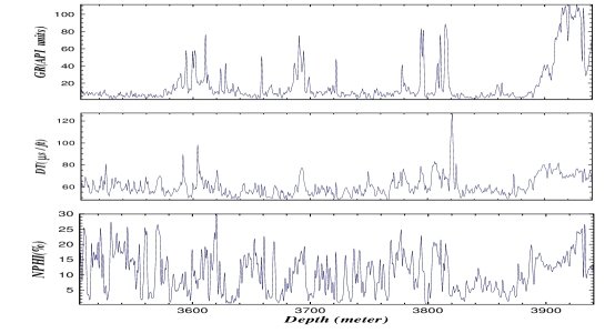
Figure 1: Three petrophysical quantities from up to down: Gamma ray (GR), sonic transient time (DT), Neutron porosity (NPHI) and depth that measured in space interval $15.4\,cm$ at depth $3504.5\,m$ to $3946.8\,m$ of a gas well in southwest of Iran.

We use well log data from a gas well in southwest of Iran. These data are Gamma ray radioactivity (GR), sonic transient time (DT) and Neutron porosity (NPHI) taken every $15.4\,cm$ at the depth interval of $3504.5-3946.8$ meters. The logged interval includes Asmari formation which is one of the main oil producer formations in Iran reservoirs and consists mainly of fractured carbonate, sand stone, shaly sand and a trace of anhydrate. Fig. $1$ shows GR, DT and NPHI data sets from the depth, $d$, of $3504.5\,m$ to $3946.8\,m$. Our analysis is based on the increment of the petrophysical quantities shown by $\varphi(d)$ in various scales, $s$, which $x(s)=\varphi(d+s)-\varphi(d)$.

In this article we describe the petrophysical quantities using the PDF and non-Gaussian degree, $q$, based on Tsallis entropy in section $2$. We explain the connection between entropy (less of information) and the non-Gaussian factor $\lambda^{2}$ (intermittency) for these data sets in section $3$ and the conclusions are stated in section $4$.

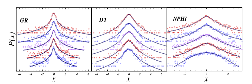
Figure 2: Increment petrophysical quantities PDF in various scales (from top to bottom) $s=15,75,225,450,900\,cm$. These estimations are fulfilled on petrophysical quantities such as Gamma emission (GR), sonic transient time (DT) and Neutron porosity (NPHI) that measured in space interval $15.4\,cm$ from a gas well in southwest of Iran. Solid lines are theoretical estimation achieved by fitting data sets to Eq. $(5)$.

II probability distribution function using entropy $S_{q}$

Since the Shannon entropy is the logarithm of the probability, the entropy is extensive. As known the Shannon entropy is considering all phenomenon based on the Boltzmanian probability distribution function (PDF). While, in general the experimental systems have no reason to obey the Boltzmanian distribution. Tsallis added a power of $q$ to the probability to be able to generalize the Shannon Entropy to all phenomenon, this causes the entropy not to be extensive. As the value of $q$ increases, the effects of the tails become more pronounced. Hence, in systems where $q$ is greater than unity the minority is more pronounced compared a Gaussian ($q=1$) system. In other words having the value of $q$ greater than unity, non-Gaussianity appears.

In order to determine the non-Gaussian degree of the system, $q$, it is essential to determine the probability distribution function analytically. Following the formalism of k ; m , we obtain the probability distribution function. Since the most probable distribution corresponds to the maximum entropy, the variational principle is applied to $S_{q}$. The continuous version of $S_{q}$ is stated as:

$$S_{q}=k\frac{1-\int{[P(x)]^{q}dx}}{q-1},$$ (3)

where $\int{P(x)dx}=1$ is the natural constraint corresponding to the normalization of Eq. $(3)$ and

$$\int{x\frac{[P(x)]^{q}}{\int{[P(x)]^{q}dx}}dx}\equiv\langle x\rangle_{q}=\overline{\mu}_{q},\,\,\,\,\ \int{(x-\overline{\mu}_{q})^{2}\frac{[P(x)]^{q}}{\int{[P(x)]^{q}dx}}dx}\equiv\langle(x-\overline{\mu}_{q})^{2}\rangle_{q}=\overline{\sigma}_{q},$$ (4)

are the natural constraints corresponding to the generalized and mean variance of $x$ respectively, see k .

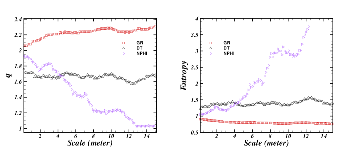
Figure 3: Left panel: the scale dependence of non-Gaussian degree, $q$, for the $3$ data sets. This estimation has been made by determining the PDF based on Tsallis entropy then exert $\chi^{2}$ test method. Right panel: representation of entropy vs. the scales by employing the definition of Tsallis entropy Eq. $(3)$ for GR (square), DT (delta) and NPHI (right triangle).

Implementing the Lagrange method in order to find the optimizing distribution under the constraints, we obtain k

$$P(x)=A_{q}[1+(q-1)B_{q}(x-\overline{\mu}_{q})^{2}]^{\frac{1}{1-q}}\ ,\ (q<3),$$ (5)

where

$$A_{q}=\left\{\begin{array}[]{ll}\frac{\Gamma(\frac{5-3q}{2-2q})}{\Gamma(\frac{2-q}{1-q})}\sqrt{\frac{1-q}{\pi}B_{q}}&\ \ \hbox{$q<1$}\\ \frac{\Gamma(\frac{1}{q-1})}{\Gamma(\frac{2-q}{2q-2})}\sqrt{\frac{q-1}{\pi}B_{q}}&\ \ \hbox{$q>1$}\end{array}\right.\ \ \ \&\ \ \ B_{q}=[(3-q)\overline{\sigma}_{q}^{2}]^{-1}.$$ (6)

In order to characterize the non-Gaussian degree of the system, $q$, the $\chi^{2}$ test method is employed. If $q$ is close to $1$, the PDF tends to be Gaussian, hence, an uncorrelated series is expected. On the other hand, the large value of the non-Gaussian factor $q$, illustrates strong correlations and similarity of neighbors in data sets which affects the behavior of the system. Therefore it can be concluded that high $q$ is a hallmark of having information about the system. For any $q$ a PDF could be plotted as shown in Fig. $2$. In Fig. $2$ the PDF is plotted using Eq. $(5)$ (solid curves) and the data sets (symbols), showing a satisfactory consistency. To state more specifically, in order to estimate $q$, we use the likelihood method which works by minimizing the parameter $\chi^{2}$ which defined as:

$$\chi^{2}(q)=\sum_{x}\frac{[P_{emperical}(x)-P(x,q)]^{2}}{\sigma^{2}_{emperical}(x)+\sigma^{2}_{q}(x)},$$ (7)

where $P_{empirical}(x)$ is computed directly from the empirical series and $P(x,q)$ is given by Eq. (5). $\sigma_{empirical}$ is the mean standard deviation of $P_{empirical}(x)$ and $\sigma_{q}$ is associated with the probability density function derived by Eq. (5). The global minimum value of $\chi^{2}$ corresponds to the best value of $q$. The best estimation of $q$, corresponding to Eq. (5), yields the PDF which fits well to the empirical PDF.

The entropy index $q$ versus the scales is shown in Fig. $3$ (left panel) for any specific petrophysical series. Note that the system is described by a specific $q$ for any scale. Taking a close look at Fig. $2$ and Fig. $3$ we deduce that the non-Gaussian PDF corresponds to large $q$, specially at small scales. This means that $q$ is showing the efficiency of non-Guassianity. As seen in the three panels of Fig. $2$, non-Gaussianity of GR is more pronounced in comparison to DT and NPHI. Hence, powerful correlations and large fluctuations in the series are observed which influence the other quantities and gives an insight to the formation of the system. However, it could be seen in the third panel which is for NPHI, that the PDF is non-Gaussian at small scales but tends to be Gaussian at large scales which corresponds to large and small values of $q$ respectively. As the values of $q$ in NPHI tends to $1$, no correlation exists, hence no information about the porosity would be available Jafari .

In the right panel of Fig. $3$, the entropy of the data sets are plotted vs. the scales. It is shown that the entropy of GR has its least value at all scales, meaning that we have fine information about the existence of shaly layers detected by gamma ray. Hence, the entropy decreases as the scale increases. Also it is shown that the entropy of NPHI is small at small scales which proves the existence of local correlation, but increases for large scales. This expresses the separated and uncorrelated porosity. Comparing Fig.$2$ and Fig. $3$ we deduce that small entropy corresponds to non-Gaussian PDF. note that this result is always true specially when the scale is small.

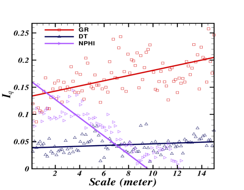
Figure 4: Relevance between difference information of petrophysical quantities contain GR (square), DT (delta), NPHI (right triangle) and scale according to Eq. $8$. Solid lines display linear fitting corresponding to the mentioned quantities.

In order to show the multifractal characteristic of the data sets the Tsalis difference information needs to be calculated n ; o

$$I_{q}(p:p_{0})=\frac{1}{1-q}[1-\int{p^{q}p_{0}^{1-q}dx}],$$ (8)

where transition is performed between states $p$ and $p_{0}$. Since the generalized entropy $S_{q}$ (Eq. $(2)$) has been introduced based on the concept of multifractals, so the degree of multifractality corresponds to the information evolution. Actually, because the phase space of a multifractal geometry is occupied heterogeneously, we expect high information rate in this system. In Fig.$4$, it is shown that the difference information received from GR is high and increasing when the scale becomes greater, that is a hallmark of strong multifractality across the scales. On the other hand, the difference information for NPHI is rapidly descending, meaning that the information at large scales is lost. Note that weak difference information for DT suggests that DT may be nearly monofractal s ; t .

III Connection between the non-Gaussian degree and intermittency

To describe the PDF of the velocity difference between two points in fully developed turbulent flows, Castaing et al. p introduced the following equation based on a log-normal cascade model q :

$$P_{\lambda,\sigma_{0}}(x)=\int_{0}^{\infty}\frac{1}{\sqrt{2\pi}\lambda}exp(-\frac{\ln^{2}(\sigma/\sigma_{0})}{2\lambda^{2}})\times\frac{1}{\sqrt{2\pi}\sigma}exp(\frac{-x^{2}}{2\sigma^{2}})d(\ln\sigma),$$ (9)

where $\lambda$, $\sigma_{0}$ are positive parameters. By taking the limit $\lambda\rightarrow 0$ in Eq. $(12)$, a Gaussian distribution is obtained. As verified in r , the shape of $P_{\lambda}$ is mainly determined by $\lambda^{2}=\langle(\delta\ln\sigma)^{2}\rangle$. In fact $\lambda^{2}$ quantifies how fatal the non-Gaussianity of data sets are u ; w ; w1 . As in the case where $q$ determined the non-Gaussian property, see Eq. $(6)$.

In Fig.$5$ the behavior of the entropy for data sets is plotted vs. $q$ and $\lambda^{2}$ in the left and right panels, respectively. since entropy is a measure of lack of information, the system with low entropy is eager to receive more information potential. This reveals that the non-Gaussian factor $\lambda^{2}$ is a sign of a sudden phase transient in the system. Meaning that the system has two phases which is a logical reason to get close to a petroleum reservoir. As seen for Gamma ray series in Fig.$5$, at high $\lambda^{2}$ the entropy tends to decrease to show the existence of global correlation with a strong interaction with environment. In fact the increase in the $\lambda^{2}$ leads to a non-Gaussian PDF. This confirms a high $q$ which results in having valuable information about the quantity. In contrast, there is high value of entropy at low $\lambda^{2}$ for NPHI which may be due to the Gaussian behavior and loss of the information of porosity.

IV Conclusions

There are systems in which long-ranged correlations give rise to strong interactions with environment and violate ergodicity. These systems can not be described by classical BG statistics. Thus another definition for entropy which is the basis of statistical mechanics was defined by Tsallis in $1988$. In this research the statistical mechanics based on the approach introduced by Tsallis was applied for analyzing petrophysical quantities which contain Gamma emission (GR), sonic transient time (DT) and Neutron porosity (NPHI). Based on the Tsallis entropy, we fitted the data sets to the probability density function (PDF) in order to obtain the non-Gaussian degree, $q$ of each series which is able to describe any system at any scale.

There exist various indicators to analysis the petroleum reservoirs. In this article, we have investigated the non- Gaussianity (uncertainly) in some indicators which could be appeared near the interface by two environments. Then, compared this effect in some indicators in various scales and measures the information contained in each indicators.

In Fig. $3$ we showed that large degree of $q$ relates to a fat-tailed PDF in Fig. $2$ which exhibits global correlation in the formation of the system. For the GR the fat tailed PDF was shown, however, for NPHI the fat tailed PDF was observed at small scales. This is due to the fact that the local correlation in NPHI exists. Hence, for DT and NPHI, $q$ and the efficiency of non-Gaussianity decreases.

Non-Gaussian PDF at large scales gives us information about the criticality in the system which results in the entropy decreases. The extremely increase of entropy for NPHI at large scales is due to the Gaussian behavior of PDF which causes separated and uncorrelated porosity. The non-Gaussian factor (intermittency) $\lambda^{2}$, which is also another important quantity is obtained from the Castaing equation. High $\lambda^{2}$ is a sign of two phases in the system which corresponds to a fat-tailed PDF or in other words a large $q$. This means that high $\lambda^{2}$ for GR at all scales gives us valuable information about the existence of global correlation and a sudden phase transition in this series. The difference information of the data sets was shown in Fig. $4$. we showed that GR has a high difference information specially at large scales. In addition, it was shown that GR exhibits a multifractal property, which is due to the fact that a high information rate in a system is present. While for DT, a monofractal property was exhibited which is due to the low information rate.

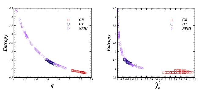
Figure 5: illustration of the entropy (Eq. ($2$)) for the data sets: GR (square), DT (delta), NPHI (right triangle) vs. non-Gaussian degree, $q$ in the right panel and the intermittency $\lambda^{2}$ defined by Castaing equation in log-normal cascade model (Eq. ($9$))in the left panel.

References

- (1) M. Fedi, D. Fiore, M. La Manna, Regularity analysis Applied to well (2005).
- (2) J. L. Jensen, L. W. Lake, P.W.M. Corbett, D.J. Goggin, Statistics for Petroleum Engineers and Geoscientists, 2nd ed., Prentice Hall, New Jersey, (2000).
- (3) M. Sahimi, Flow and Transport in Porous Media and Fractured Rock, 2nd ed., Wiley-VCH, Berlin, (2011).
- (4) G. Reza Jafari, Muhammad Sahimi, M. Reza Rahimi Tabar, M. Reza Rasaei, Phys. Rev. E 83, 026309 (2011).
- (5) R.B. Ferreira, V.M. Vieira, I. Gleria, M.L. Lyra, Physica A 388, 747 (2009).
- (6) M. Sahimi, S.E. Tajer, Phys. Rev. E 71 (2005) 046301.
- (7) E. Fermi, Thermodynamics, (Doubliday, New York) (1936).
- (8) C. Tsallis, Euro. Phys. J. A 40, 257 (2009).
- (9) L. Boltzmann , Lectures on Gas Theory, (Dover, New York) (1995).
- (10) K. Huang, Statistical Mechanics, (John Wiley and Sons, New York) (1963).
- (11) C. Tsallis, Introduction to Nonextensive Statistical mechanics, Approaching a Complex World, (Springer Science+Business Media, New York), (2009).
- (12) S. M. D. Queiros, L. G. Moyano, J. de Souza, C. Tsallis, Eur. Phys. J. B 55, 161 (2007).
- (13) C. Tsallic, J. Stat. Phys 52, 479 (1988).
- (14) E. M. F. Curdao, C. Tsallis, J. Phys. A 24, L69 (1991); Corrigenda 24, 3187 (1991); 25, 1019 (1992).
- (15) B. Lesche, J. Stat. Phys. 27, 419 (1982).
- (16) M.Gell-Mann, C. Tsallis Nonextensive entropy-Interdisciplinary Applications, (Oxford University Press, New York, 2004).
- (17) V. Latore, M. Baranger, Phys. Rev. Lett. 273, 97 (1999).
- (18) L. Telesca, Physica A 389, 1911 (2010).
- (19) L. Telesca, Terra Nova 22, 87 (2010)
- (20) L. Telesca, Tectonophysics 494, 155 (2010).
- (21) C. Tsallis, R. S. Mendes, A. R. Plastino, Phys. A 261, 534 (1998).
- (22) C. Tsallis, Phys. Rev. E 58, 1442 (1998).
- (23) R. G. Zaripov, Russian. Phys. J, 44, 1159 (2001).
- (24) H. Dashtian, G. R. Jafari, Z. Koohi, M. Masihi, M. Sahimi, Transport in Porous Media (2011).
- (25) H. Dashtian, G. R. Jafari, M. Sahimi, M. Masihi, Physica A 390, 2096 (2011).
- (26) B. Castaing, Y. Gagne, E. J. Hopfinger, Physica D 46, 177 (1990).
- (27) K. Kiyono, Z. R. Struzik, Y. Yamamoto, Phys. Rev. E 76, 041113 (2007).
- (28) B. Chabaud, A. Naert, J. Peinke, F. Chilla, B. Castaing, B. Hebral, Phys. Rev. Lett 73, 3227 (1994).
- (29) G. R. Jafari, M. Sadegh Movahed, P. Noroozzadeh, F. Ghasemi, M. Sahimi, M. R. Rahimi Tabar, International Journal of Modern Physics C 18, 1689 (2007).
- (30) F. Shayeganfar, S. Jabbari-Farouji, M.Sadegh Movahed, G. R. Jafari, M. Reza Rahimi Tabar, Phys. Rev. E 80, 061126 (2009).
- (31) F. Shayeganfar, S. Jabbari-Farouji, M. Sadegh Movahed, G. R. Jafari, M. R. Rahimi Tabar, Phys. Rev. E 81, 061404 (2010).