11email: sanjose@strw.leidenuniv.nl 22institutetext: Max Planck Institut für Extraterrestrische Physik, Giessenbachstrasse 2, 85478 Garching, Germany. 33institutetext: SRON Netherlands Institute for Space Research, PO Box 800, 9700 AV Groningen, The Netherlands 44institutetext: Kapteyn Astronomical Institute, University of Groningen, PO Box 800, 9700 AV Groningen, The Netherlands 55institutetext: Université de Bordeaux, Observatoire Aquitain des Sciences de l’Univers, 2 rue de l’Observatoire, BP 89, F-33270 Floirac Cedex, France 66institutetext: CNRS, LAB, UMR 5804, Laboratoire d’Astrophysique de Bordeaux, 2 rue de l’Observatoire, BP 89, F-33270 Floirac Cedex, France 77institutetext: Department of Astronomy, The University of Michigan, 500 Church Street, Ann Arbor, MI 48109-1042, USA 88institutetext: University of Waterloo, Department of Physics and Astronomy, Waterloo, Ontario, Canada 99institutetext: Max-Planck-Institut für Radioastronomie, Auf dem Hügel 69, 53121 Bonn, Germany 1010institutetext: National Research Council Canada, Herzberg Institute of Astrophysics, 5071 West Saanich Road, Victoria, BC V9E 2E7, Canada 1111institutetext: Department of Physics and Astronomy, University of Victoria, Victoria, BC V8P 1A1, Canada
Herschel-HIFI observations of high-J CO and isotopologues in star-forming regions: from low- to high-mass††thanks: Herschel is an ESA space observatory with science instruments provided by European-led Principal Investigator consortia and with important participation from NASA.
Abstract
Context.
Our understanding of the star formation process has traditionally been confined to certain
mass or luminosity boundaries because most studies focus only on
low-, intermediate-
or high-mass star-forming regions. Therefore, the processes that regulate the formation of these
different objects have not been effectively linked.
As part of the “Water In Star-forming regions with Herschel” (WISH) key program, water and other important
molecules, such as CO and OH, have been observed in 51 embedded young stellar objects (YSOs).
The studied sample covers a range of luminosities from to L⊙.
Aims. We analyse the CO line emission towards a large sample of embedded protostars in terms of both
line intensities and profiles.
This analysis covers a wide luminosity range in order to achieve a better understanding of
star formation without imposing luminosity boundaries. In particular, this paper aims to
constrain the dynamics of the environment in which YSOs form.
Methods. Herschel-HIFI spectra of the 12CO =10–9, 13CO =10–9 and
C18O =5–4, =9–8 and
=10–9 lines are analysed for a sample of 51 embedded protostars. In addition, JCMT spectra of
12CO =3–2 and C18O =3–2 extend this analysis to
cooler gas components.
We focus on characterising the shape and intensity of the CO emission line profiles
by fitting the lines with one or two Gaussian profiles.
We compare the values and results of these fits across the entire luminosity range
covered by WISH observations. The effects of
different physical parameters as a function of luminosity and the
dynamics of the envelope-outflow
system are investigated.
Results. All observed CO and isotopologue spectra show a strong linear correlation between
the logarithms of the line and bolometric luminosities across six orders of magnitude on both axes.
This suggests that the high- CO lines primarily trace the amount of dense gas associated with YSOs and
that this relation can be extended to larger (extragalactic) scales.
The majority of the detected 12CO line profiles can be decomposed into a broad and a narrow Gaussian component,
while the C18O spectra are mainly fitted with a single Gaussian.
For low- and intermediate-mass protostars, the width of the
C18O =9–8 line is roughly twice that of the C18O =3–2 line, suggesting increased
turbulence/infall in the warmer inner envelope. For high-mass protostars, the line widths are comparable
for lower- and higher- lines.
A broadening of the line profile is also observed from pre-stellar cores to embedded protostars, which is due
mostly to non-thermal motions (turbulence/infall).
The widths of the broad 12CO =3–2 and =10–9 velocity components
correlate with those of the narrow
C18O =9–8 profiles, suggesting that the entrained outflowing gas
and envelope motions are related independent of the mass of the protostar.
These results indicate that physical processes in protostellar envelopes have similar
characteristics across the studied luminosity range.
Key Words.:
Astrochemistry –– Stars: formation –– Stars: protostars –– ISM: molecules –– ISM: kinematics and dynamics –– line: profiles1 Introduction
The evolution of a protostar is closely related to the initial mass of the molecular core from which it forms and to the specific physical and chemical properties of the original molecular cloud (e.g., Shu et al. 1993; van Dishoeck & Blake 1998; McKee & Ostriker 2007). During the early stages of their formation, young stellar objects (YSOs) are embedded in large, cold and dusty envelopes which will be accreted or removed by the forming star. Depending on the mass of the star-forming region, the parameters and mechanisms that rule several processes of the star formation, such as driving agent of the molecular outflow and accretion rates, will vary.
Molecular outflows are crucial for removing angular momentum and mass from the protostellar system (see review by Lada 1999). They have been extensively studied for low-mass YSOs (e.g., Cabrit & Bertout 1992; Bachiller & Tafalla 1999) where they are better characterised than for massive protostars (e.g., Shepherd & Churchwell 1996; Beuther & Shepherd 2005). The reason is related to the short life-time (Mottram et al. 2011) and the large distances (few kpc) associated with massive YSOs. This means that outflows from massive stars are less well resolved than their low-mass counterparts. The agent that drives the molecular outflow, either jets or winds from the disk and/or stars (e.g., Churchwell 1999; Arce et al. 2007), might be different depending on the mass of the star-forming region. Therefore, the interaction of the outflow with the surrounding material and especially the resulting chemistry may differ across the mass range.
The accretion rates are also different depending on the mass of the forming star. Typical values for low-mass star formation are 10-7–10-5 M⊙ yr-1 (Shu 1977; Bontemps et al. 1996) whereas higher values are necessary in order to overcome radiation pressure and form massive stars within a free-fall time (e.g., Jijina & Adams 1996). These values range from 10-4 to 10-3 M⊙ yr-1 for sources with L⊙ (e.g., Beuther et al. 2002). In addition, for the low-mass sources, the accretion episode finishes before the protostar reaches the main sequence, while massive YSOs still accrete circumstellar material after reaching the hydrogen burning phase (Palla & Stahler 1993; Cesaroni 2005).
Another difference is that the ionising radiation created by main-sequence OB stars is much more powerful than that generated by a single low-mass protostar. Therefore, photon dominated regions (PDR) and Hii regions are formed in areas of massive star formation, affecting the kinematics, temperature and chemistry of the surrounding material (Hollenbach & Tielens 1999). In addition, the strength of stellar winds and their interaction with the envelope material is different depending on the stellar spectral type of the YSOs.
Because of these differences, the study of star formation has traditionally been restricted to mass boundaries, focused either on low-mass ( 3 M⊙) or high-mass ( 8 M⊙) YSOs. One of the goals of the “Water In Star-forming regions with Herschel” (WISH) key program (van Dishoeck et al. 2011) is to offer a complete description of the interaction of young stars with their surroundings as a function of mass. For this purpose, and in order to constrain the physical and chemical processes that determine star formation, water and other key molecules like CO have been observed for a large sample of embedded YSOs (51 sources). The targeted objects cover a vast range of luminosities (from 1 L⊙ to 105 L⊙) and different evolutionary stages (more details in Section 2.1). With the Heterodyne Instrument for the Far-Infrared (HIFI; de Graauw et al. 2010) on board the Herschel Space Observatory (Pilbratt et al. 2010), high spectral resolution data of high frequency molecular lines have been obtained. These can be used to probe the physical conditions, chemical composition and dynamics of protostellar systems (e.g., Evans 1999; Jørgensen et al. 2002; van der Wiel et al. 2013, submitted).
Due to its high, stable abundance and strong lines, CO is one of the most important and often used molecules to probe the different physical components of the YSO environment (envelope, outflow, disk). In particular, molecular outflows are traced by 12CO emission through maps in the line wings (e.g, Curtis et al. 2010). Its isotopologue C18O is generally thought to probe quiescent gas in the denser part of the protostellar envelope, whereas 13CO lines originate in the extended envelope and the outflow cavity walls (e.g., Spaans et al. 1995; Graves et al. 2010; Yıldız et al. 2012). In addition, CO has a relatively low critical densities, due to its small permanent dipole moment (0.1 Debye), and relatively low rotational energy levels, so this molecule is easily excited and thermalised by collisions with H2 in a typical star formation environment. For this reason, measurements of CO excitation provide a trustworthy estimate of the gas kinetic temperature. Moreover, integrated intensity measurements can be used to obtain column densities of warm gas, providing a reference to determine the abundances of other species, such as water and H2.
Most CO observations from ground-based sub-millimetre telescopes have been limited to low- rotational transitions (up to upper transition =3, i.e., upper-level energy 35 K), or mid- transitions (=6, with a of 100 K). Thanks to HIFI, spectrally resolved data for high- CO transitions ( up to 16, 600 K) are observable for the first time, so warm gas directly associated with the forming star is probed (e.g., Yıldız et al. 2010, 2012; Plume et al. 2012; van der Wiel et al. 2013, submitted). Therefore, a uniform probe of the YSOs over the entire relevant range of (from 10–600 K) is achieved by combining HIFI data with complementary spectra from single-dish ground-based telescopes. These observations are indispensable in order to ensure a self-consistent data set for analysis. Finally, the study of these lines in our Galaxy is crucial in order to compare them with the equivalent lines targeted in high-redshift galaxies which are often used to determine star-formation rates on larger scales.
In this paper we present 12CO =10–9, 13CO =10–9, C18O =5–4, =9–8 and =10–9 HIFI spectra of 51 YSOs. Complementing these data, 12CO and C18O =3–2 spectra observed with the James Clerk Maxwell Telescope (JCMT) are included in the analysis in order to use CO to its full diagnostic potential and extend the analysis to different regions of the protostellar environment with different physical conditions. Section 2 describes the sample, the observed CO data and the method developed to analyse the line profiles. A description of the morphology of the spectra, an estimation of the kinetic temperatures and correlations regarding the line luminosities of each isotopologue transition are presented in Section 3. These results are also compared to other YSO parameters such as luminosity and envelope mass. In Section 4 we discuss the results to constrain the dynamics of individual velocity components of protostellar envelopes, characterise the turbulence in the envelope-outflow system and consider high- CO as a dense gas tracer. Our conclusions are summarised in Section 5.
2 Observations
2.1 Sample
The sample discussed in this paper is drawn from the WISH survey and covers a wide range of luminosities and different evolutionary stages. A total of 51 sources are included in this study, which can be classified into three groups according to their bolometric luminosities, . The sub-sample of low-mass YSOs, characterized by 50 L⊙, is composed of 15 Class 0 and 11 Class I protostars (see Evans et al. 2009 for details of the classification). Six intermediate-mass sources were observed with 70 L⊙ 2103 L⊙. Finally, 19 high-mass YSOs with 103 L⊙ complete the sample. The bolometric luminosity of the sample members, together with their envelope masses (), distances () and source velocities () are summarised in Table 1. For more information about the sample studied in WISH, see van Dishoeck et al. (2011). Focusing on the evolutionary stages, the sub-sample of low-mass YSOs ranges from Class 0 to Class I, the intermediate-mass objects from Class 0 to Class I as well, and in the case of the high-mass sources, from (mid-IR-quiet/mid-IR-bright) massive young stellar objects (MYSOs) to ultra-compact H ii regions (UCH ii).
| Source | References | ||||
| (km s-1) | () | (kpc) | () | ||
| Low-mass: Class 0 | |||||
| L 1448-MM | 9.0 | 0.235 | 3.9 | 1 | |
| NGC 1333 IRAS 2A | 35.7 | 0.235 | 5.1 | 1 | |
| NGC 1333 IRAS 4A | 9.1 | 0.235 | 5.6 | 1 | |
| NGC 1333 IRAS 4B | 4.4 | 0.235 | 3.0 | 1 | |
| L 1527 | 1.9 | 0.140 | 0.9 | 1 | |
| Ced110 IRS4 | 0.8 | 0.125 | 0.2 | 1 | |
| BHR 71 | 14.8 | 0.200 | 2.7 | 1 | |
| IRAS 15398 | 1.6 | 0.130 | 0.5 | 1 | |
| L 483-MM | 10.2 | 0.200 | 4.4 | 1 | |
| Ser SMM 1 | 30.4 | 0.230 | 16.1 | 1 | |
| Ser SMM 4 | 1.9 | 0.230 | 2.1 | 1 | |
| Ser SMM 3 | 5.1 | 0.230 | 3.2 | 1 | |
| L 723-MM | 3.6 | 0.300 | 1.3 | 1 | |
| B 335 | 3.3 | 0.250 | 1.2 | 1 | |
| L 1157 | 4.7 | 0.325 | 1.5 | 1 | |
| Low-mass: Class I | |||||
| L 1489 | 3.8 | 0.140 | 0.2 | 1 | |
| L 1551 IRS 5 | 22.1 | 0.140 | 2.3 | 1 | |
| TMR 1 | 3.8 | 0.140 | 0.2 | 1 | |
| TMC 1A | 2.7 | 0.140 | 0.2 | 1 | |
| TMC 1 | 0.9 | 0.140 | 0.2 | 1 | |
| HH 46 | 27.9 | 0.450 | 4.4 | 1 | |
| IRAS 12496 | 35.4 | 0.178 | 0.8 | 1 | |
| Elias 29 | 14.1 | 0.125 | 0.3 | 1 | |
| Oph IRS 63 | 1.0 | 0.125 | 0.3 | 1 | |
| GSS 30 IRS1 | 13.9 | 0.125 | 0.6 | 1 | |
| RNO 91 | 2.6 | 0.125 | 0.5 | 1 | |
| Intermediate-mass | |||||
| NGC 7129 FIRS 2 | 9.8 | 430 | 1.25 | 50.0 | 2 |
| L1641 S3 MMS1 | 5.3 | 70 | 0.50 | 20.9 | 2 |
| NGC 2071 | 9.6 | 520 | 0.45 | 30.0 | 2 |
| Vela IRS 17 | 3.9 | 715 | 0.70 | 6.4 | 2 |
| Vela IRS 19 | 12.2 | 776 | 0.70 | 3.5 | 2 |
| AFGL 490 | 13.5 | 2000 | 1.00 | 45.0 | 2 |
| High-mass | |||||
| IRAS05358+3543 | 17.6 | 1.8 | 142 | 3 | |
| IRAS162724837 | 46.2 | 3.4 | 2170 | 3 | |
| NGC6334-I(N) | 3.3 | 1.7 | 3826 | 3 | |
| W43-MM1 | 98.8 | 5.5 | 7550 | 3 | |
| DR21(OH) | 3.1 | 1.5 | 472 | 3 | |
| W3-IRS5 | 38.4 | 2.0 | 424 | 3 | |
| IRAS180891732 | 33.8 | 2.3 | 172 | 3 | |
| W33A | 37.5 | 3.8 | 1220 | 3 | |
| IRAS181511208 | 32.8 | 3.0 | 153 | 3 | |
| AFGL2591 | 5.5 | 3.3 | 320 | 3 | |
| G3270.6 | 45.3 | 3.3 | 2044 | 3 | |
| NGC6334-I | 7.4 | 1.7 | 500 | 3 | |
| G29.960.02 | 97.6 | 6.0 | 768 | 3 | |
| G31.41+0.31 | 97.4 | 7.9 | 2968 | 3 | |
| G5.890.39 | 10.0 | 1.3 | 140 | 3 | |
| G10.47+0.03 | 67.3 | 5.8 | 1168 | 3 | |
| G34.26+0.15 | 58.0 | 3.3 | 1792 | 3 | |
| W51N-e1 | 59.5 | 5.1 | 4530 | 3 | |
| NGC7538-IRS1 | 56.2 | 2.7 | 433 | 3 |
Notes. See van Dishoeck et al. (2011) for the source coordinates.
References.
(1) Bolometric luminosities and envelope masses obtained from Kristensen et al. (2012).
(2) Envelope masses collected in Wampfler et al. (2013, in press).
(3) Bolometric luminosities (obtained from observations) and envelope masses calculated in
van der Tak et al. (2013, submitted).
2.2 HIFI observations
The sources were observed with the Heterodyne Instrument for the Far Infrared (HIFI) on the Herschel Space Observatory. The HIFI CO and isotopologue lines studied in this paper are: 12CO =10–9, 13CO =10–9, C18O =5–4, =9–8 and =10–9. The upper-level energies and frequencies of these lines together with the HIFI bands, main beam efficiencies (), beam sizes, spectral resolution and integration times are presented in Table 2. With the exception of the 12CO =10–9 line, all isotopologue line observations were obtained together with H2O lines. The 12CO =10–9 line was targeted for the low- and intermediate-mass sample but only for one high-mass object (W3-IRS5). The 13CO =10–9 and C18O =9–8 lines were observed for the entire sample, while C18O =5–4 only for the Class 0 and intermediate-mass protostars. C18O =10–9 was observed for all low-mass Class 0 sources, two low-mass Class I (Elias 29 and GSS 30 IRS1), one intermediate-mass YSO (NGC 7129) and the entire high-mass sub-sample.
Single-pointing observations were performed for all targets in dual-beam-switch (DBS) mode, chopping to a reference position 3 from the target. There is no contamination due to emission at the off position except for the 12CO =10–9 spectrum of NGC1333 IRAS2A and IRAS4A (see Yıldız et al. 2010 for more details). These spectra have been corrected and presented in this paper without contamination. In the case of W43-MM1, the absorption features found in the 13CO =10–9 spectrum are caused by H2O+ (Wyrowski et al. 2010).
HIFI has two backends: the Wide Band Spectrometer (WBS) and the High Resolution Spectrometer (HRS). Both spectrometers simultaneously measure two polarizations, horizontal (H) and vertical (V). For more details, see Roelfsema et al. (2012). The WBS has a constant spectral resolution of 1.1 MHz, whereas the HRS has different configuration modes with four possible spectral resolutions: 0.125, 0.25, 0.5 and 1.0 MHz. The spectral resolution for each of the studied HIFI lines is listed in Table 2. The WBS data present lower noise than the HRS data (factor of ) and provide a good compromise between noise and resolution. Therefore, the WBS data are the primary focus of this paper. HRS observations are only used for analysing the C18O =5–4 line for the low-mass sources because their narrow line profiles require the higher spectral resolution provided by these data.
The data reduction was performed using the standard HIFI pipeline in the Herschel Interactive
Processing Environment (HIPE111HIPE is a joint development by the Herschel Science Ground Segment
Consortium, consisting of ESA, the NASA Herschel Science Centre, and the HIFI, PACS and SPIRE consortia.)
ver. 8.2 (Ott 2010), resulting in absolute calibration on the corrected antenna temperature
scale, and velocity calibration with a precision of a few m s-1.
The version of the calibration files used is 8.0, released in February 2012.
The flux scale accuracy was estimated to be 10% for bands 1, 4 and 5.
Subsequently, the data were exported to
GILDAS-CLASS222http://www.iram.fr/IRAMFR/GILDAS/
for further analysis. The H and V polarizations were observed simultaneously
and the spectra averaged to improve the signal-to-noise ratio.
In order to avoid possible discrepancies between both signals, the two polarisations were inspected
for all the spectra presented in this paper with no differences 20% found.
Afterwards, line intensities were converted to main-beam brightness temperatures through the
relation (see Wilson et al. 2009
for further information about radio-astronomy terminology).
The main beam efficiency, , for each HIFI band was taken from Roelfsema et al. (2012)
and listed in Table 2.
The final step of the basic reduction was the subtraction of a
constant or linear baseline.
2.3 JCMT ground-based observations
Complementary data from the 15-m James Clerk Maxwell Telescope (JCMT) on Mauna Kea, Hawaii are also included in this paper, in particular for the high-mass sources for which 12CO =10–9 data are not available. Jiggle map observations of 12CO =3–2 and C18O =3–2 for a sub-sample of YSOs were obtained with the Heterodyne Array Receiver Program (HARP, Buckle et al. 2009) in August 2011 and summer 2012 (proposal M11BN07 and M12BN06). For the sources and transitions not included in the proposal, comparable data were obtained from the JCMT public archive. Four low-mass sources were observed with the 12-m Atacama Pathfinder Experiment Telescope, APEX, because these protostars are not visible from the JCMT (see Appendix B). Further information about the low-mass YSOs and data can be found in Yıldız et al. (2013, submitted).
The HARP instrument is a pixel receiver array, although during the observation period one of the receivers (H14) was not operational. The lines were observed in position-switching mode, with the off-positions carefully chosen in order to avoid contamination. For the most massive and crowded regions, test observations of the off-position were taken for this purpose. The spatial resolution of the JCMT at the observed frequencies is 14, with a main beam efficiency of 0.63333http://www.jach.hawaii.edu/JCMT/spectralline/General/status.html. This same value of was used for the data obtained from the JCMT archive because the small variations of this parameter ( 10) recorded over time are negligible compared to the calibration uncertainties of the JCMT (20, Buckle et al. 2009). Some of the spectra collected from the JCMT archive were observed in a lower spectral resolution setting. Therefore, for these data the spectral resolution is 0.4 km s-1 instead of 0.1 km s-1 (indicated in Table 2).
In the first step of the reduction process, the raw ACSIS data downloaded from the JCMT archive were transformed
from sdf format to fits format using the
Starlink444http://starlink.jach.hawaii.edu/starlink package for each and every pixel.
Next, the data were converted to CLASS format and the central spectrum was extracted after
convolving the map
to the same beam size as the 12CO =10–9 HIFI observations (20).
Line intensities were then converted to the main-beam brightness temperature scale and linear
baselines subtracted. Since this manuscript focuses on analysing and comparing the central spectrum
of the studied YSOs, the full JCMT spectral maps will be presented and discussed in a forthcoming paper.
| Mol. | Trans. | Frequency | Tel./Inst.-band | Beam | Spec. Resol. | Exposure time (min) | |||||
|---|---|---|---|---|---|---|---|---|---|---|---|
| (K) | (GHz) | size () | (km s-1) | LM0 | LMI | IM | HM | ||||
| 12CO | 3–2 | 33.2 | 345.796 | JCMT | 0.63 | 14 | 0.1/0.4 | 21 | 21 | 21 | 21 |
| 10–9 | 304.2 | 1151.985 | HIFI-5a | 0.64 | 20 | 0.13a | 10 | 7 | 10 | 20 | |
| 13CO | 3–2 | 31.7 | 330.588 | JCMT | 0.63 | 15 | 0.1/0.4 | 32 | 32 | 32 | 32 |
| 10–9 | 290.8 | 1101.350 | HIFI-4b | 0.74 | 21 | 0.14a | 40 | 30 | 40 | 42/59 | |
| C18O | 3–2 | 31.6 | 329.331 | JCMT | 0.63 | 15 | 0.1/0.4 | 39 | 39 | 24 | 24 |
| 5–4 | 79.0 | 548.831 | HIFI-1a | 0.76 | 42 | 0.07b | 60 | – | 31 | – | |
| 9–8 | 237.0 | 987.560 | HIFI-4a | 0.74 | 23 | 0.15a | 20 | 20 | 20 | 7 | |
| 10–9 | 289.7 | 1097.163 | HIFI-4b | 0.74 | 21 | 0.14a | 30c | 300 | 30 | 30 | |
Notes. LM0: low-mass Class 0 sources. LMI: low-mass Class I objects.
IM: intermediate-mass YSOs. HM: high-mass protostars.
(a) WBS data. (b) HRS data. (c) NGC1333 IRAS 2A, 4A and 4B were observed for 300 min each.
2.4 Decomposition method
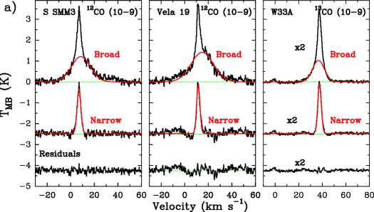
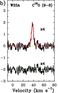
In order to quantify the parameters that fit each spectrum, the following procedure was applied to all spectra. First, the data were re-sampled to 0.27 km s-1 so that the results could be compared in a systematic manner. Then, the spectra were fitted with a single Gaussian profile using the IDL function mpfitfun, after which we plotted the residuals obtained from the fit to confirm whether the line profile hid an additional Gaussian component. For those sources whose profiles showed clear sub-structure, i.e., the residuals were larger than 3 sigma rms, a two Gaussian component fit was used instead. Examples of the decomposition procedure are shown in Fig. 1. The results of this process together with the rms and integrated intensity for all lines are presented in Tables 5 to 9 in Appendix A.
All HIFI lines are observed in emission and none of the HIFI spectra present clear infall signatures. Moreover, some CO lines show weak self-absorption features, which are of marginal significance and will not be discussed further. In addition, extremely high velocity (EHV) emission features have been identified. The EHV components are knotty structures spaced regularly and associated with shocked material moving at velocities of hundreds of km s-1 (e.g. Bachiller et al. 1990). These structures have been detected in the 12CO =10–9 spectra for the low-mass Class 0 sources L1448-MM and BHR 71 (Kristensen et al. 2011; Yıldız et al. 2013, submitted). These EHV components were not included in the study of the line profiles, so the residuals were analysed after fitting each of these features with a Gaussian function and subtracting them from the initial profile.
The method used for examining the data is similar to that introduced by Kristensen et al. (2010) for several water lines in some of the WISH low-mass YSOs, applied to high- CO in Yıldız et al. (2010) and extended in Kristensen et al. (2012) for the 557 GHz 110–101 water line profiles of the entire low-mass sample. The emission lines are classified as narrow or broad if the full width half maximum (FWHM) of the Gaussian component is lower or higher than 7.5 km s-1, respectively. This distinction is made because 7.5 km s-1 is the maximum width obtained in the single Gaussian fit of the HIFI C18O lines, which is considered as narrow and traces the dense warm quiescent envelope material (see Section 4 for further analysis and discussion).
The narrow component identified in the high- CO isotopologue lines is always seen in emission, unlike a component of similar width seen in the 110-101 line of water (Kristensen et al. 2012). The narrow components in high- CO and low- water probe entirely different parts of the protostar: the former traces the quiescent warm envelope material, the latter traces the cold outer envelope and ambient cloud. The broad emission in low- CO is typically narrower than in water and traces entrained outflow material. Only the highest- lines observed by HIFI trace the same warm shocked gas as seen in the water lines (Yıldız et al. 2013, submitted). To summarise, the components identified in the CO and isotopologue data cannot be directly compared to those observed in the H2O 110-101 lines because the physical and chemical conditions probed by water are different to those probed by CO (see Santangelo et al. 2012; Vasta et al. 2012).
In the analysis of the JCMT data, the FWHM of the broad velocity component for the complex 12CO =3–2 line profiles was disentangled by masking in each spectrum the narrower emission and self-absorption features. The width of the narrow C18O =3–2 lines was constrained by fitting these profiles with a single Gaussian. The results of these fits are presented in Table 10 in Appendix B.
3 Results
One of the aims of this paper is to characterise how the observed emission lines compare as a function of source luminosity. In order to simplify the comparison across the studied mass range, the main properties and parameters of the HIFI and JCMT lines, such as line morphology, total intensity and kinetic temperature, are presented in this section. A more detailed description of the line profiles is reserved for Appendices A and B (Figs. 15 to 19 show the HIFI spectra and Figs. 23 and 24 the JCMT data).
Further study and analysis of each sub-sample will be presented in several forthcoming papers. The CO lines for the low-mass sources and their excitation will be discussed by Yıldız et al. (2013, submitted). A review of the intermediate-mass sources focused on the water lines will be performed by McCoey et al. (in prep.). In the case of high-mass YSOs, low- H2O line profiles will be studied in detail by van der Tak et al. (2013, submitted).
In this manuscript a summary with the main characteristics of the studied emission line profiles is presented in Section 3.1. Section 3.2 describes the calculation of the line luminosity, , for each observed isotopologue together with its correlation with . Finally, in Section 3.3, an estimation of the kinetic temperature is obtained for two sources, an intermediate-mass and a high-mass YSO, and compared with values obtained for low-mass sources.
3.1 Characterisation of the line profiles
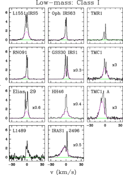
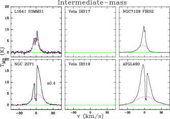
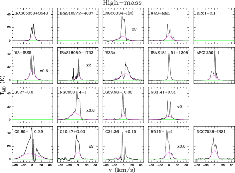
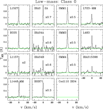
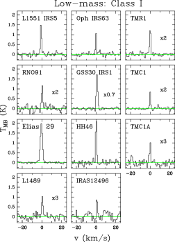
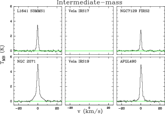
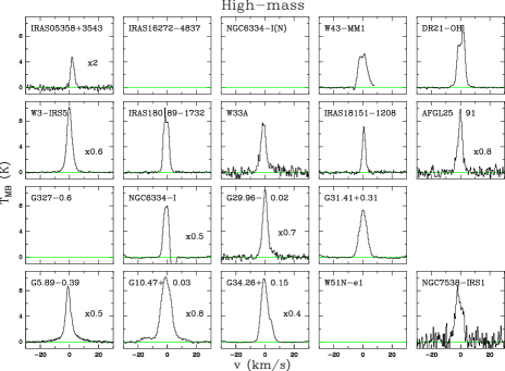
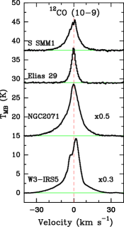
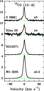
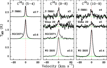
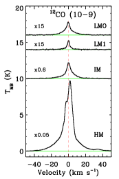
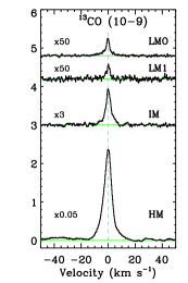
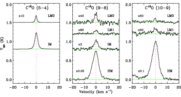
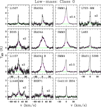
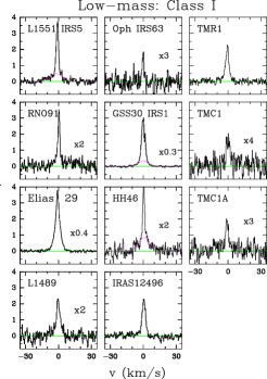
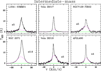
Figures 2 and 3 show characteristic profiles of each transition and YSO sub-type, so the line profiles can be compared across the luminosity range. 12CO =10–9 spectra present more intense emission lines than the other observed isotopologues and more complex line profiles. Two velocity components are identified and most of the 12CO =10–9 spectra can be well fitted by two Gaussian profiles (Fig. 1a). Weak self-absorption features are also observed in some sources, such as Ser SMM1. 13CO =10–9 profiles are weaker and narrower than 12CO =10–9 spectra. Some of the detected lines, especially for the high-mass sample, are fitted using two Gaussian components (Fig. 1a). In the case of the C18O =5–4 spectra, a weak broad velocity component is identified in 6 sources (indicated in Table 7), due to the long exposure time and the high reached for this transition. The width of this broad component is narrower by a factor of 2–3 than that detected for the 12CO and 13CO =10–9 lines. Similarly, two velocity components have been identified for the C18O =9–8 line in three high-mass sources: G10.47+0.03, W51N-e1 and G5.89-0.39 (see Fig. 19). These massive objects present the widest broad velocity components for both 13CO and C18O =10–9 spectra. The width of the broad C18O =9–8 component is slightly smaller than that identified in the 13CO =10–9 emission for each of these YSOs.
Two velocity components were previously identified in approximately half of the 20 deeply embedded young stars in the Taurus molecular cloud studied by Fuller & Ladd (2002) using lower- C18O observations. They found typical FWHM line widths of 0.6 and 2.0 km s-1 for the narrow and broad component respectively. These values are significantly narrower than the widths obtained from the HIFI data, so our interpretation and analysis of these components is different to that presented by Fuller & Ladd (2002). On the other hand, the bulk of C18O line profiles (especially =9–8 and =10–9 transitions) are generally well fitted by a single Gaussian (for an example, see Fig. 1b). Therefore, in our analysis only the narrow C18O component is considered for the three sources with two velocity component profile. Regarding the line intensity, the spectra of the observed high-mass YSOs have higher main beam temperatures than the spectra of the intermediate-mass objects, which in turn show stronger lines than the low-mass sources.
Another result obtained when we extend this characterisation to the JCMT data is the complexity of the 12CO =3–2 profiles compared to the 12CO =10–9 spectra (see Figs. 15 and 23 for comparison across the studied sample). The HIFI data probe warmer gas from inner regions of the molecular core and present simpler emission line profiles (with no deep absorptions and foreground emission features) than the lower- spectra. However, similar to the 12CO =10–9 line profiles, the 12CO =3–2 spectra can be decomposed into different velocity components. A broad velocity component is identified in 39 out of 47 sources, ranging from 7.4 to 53.5 km s-1 in width. For C18O, the shape of the =3–2 lines are very similar to those of the =9–8 lines (see Figs. 20 to 22 for examples).
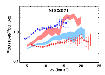
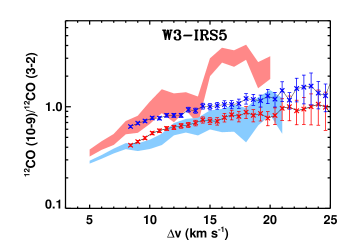
The FWHM of the 12CO =3–2 broad component for most of the high-mass sources is approximately double the width obtained for the 13CO =10–9 broad component (values in Tables 16 and 10). In the case of the one source for which a 12CO =10–9 observation was performed as part of WISH (W3-IRS5), the width of the broad component is similar to that calculated for the =3–2 spectrum (factor of 1.20.1) and is twice the width of the 13CO =10–9 emission line (see Fig. 2). Similar ratios were found by van der Wiel et al. (2013, submitted) for the high-mass source AFGL2591 as part of the CHESS (“Chemical HErschel Survey of Star-forming regions”) key program observations. For the intermediate-mass object NGC 2071, the 12CO =10–9 broad component is 1.70.1 larger than the width of the 13CO =10–9 broad component. This ratio is 1.50.4 for the one low-mass YSO for which a decomposition of the line profile can be performed in both transitions simultaneously (Ser SMM1). Thus, it appears that the 12CO =10–9 profile becomes increasingly broader compared to the 13CO =10–9 profile with increasing protostellar mass. The average ratio of the width of the broad component of the 12CO =10–9 line divided by the width of the broad component of the 12CO =3–2 line is approximately 1.00.1 for the intermediate-mass sources and 1.30.2 for the low-mass protostars.
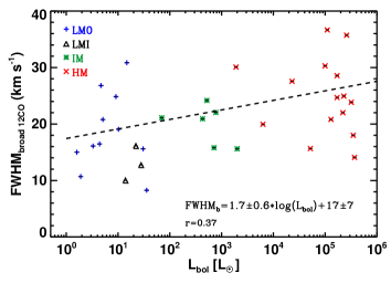
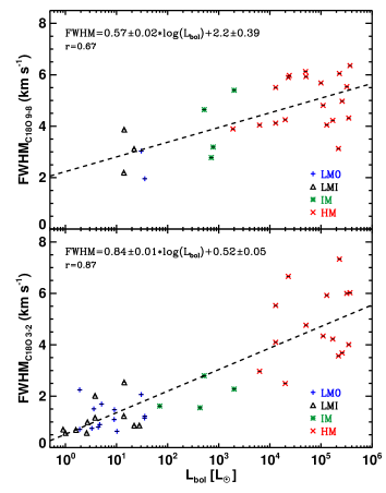
In order to compare the broad velocity component of the 12CO data with the narrow C18O line profiles across the entire studied luminosity range, the FWHM of the 12CO =3–2 spectra is used as a proxy for the FWHM of the 12CO =10–9 profiles for the high-mass sample. The widths of the fits obtained for the 12CO broad velocity components and the narrow C18O =9–8 and =3–2 lines are plotted versus their bolometric luminosities (Figs. 4 and 5). From the figure of the broad velocity component of the 12CO data we infer that the line-wings become broader from low- to high-mass. Low-mass Class 0 protostars characterised by powerful outflows, such as L1448, BHR 71 and L 1157, are the clear outstanding sources in the plot. The median FWHM of this component for each sub-group of protostars together with the calculated median of the FWHM values for the C18O =3–2 and =9–8 lines are summarised in Table 3. Even though there are only six intermediate-mass sources and the results could be sample biased, the trend of increasing width from low- to high-mass is consistent with the result obtained for intermediate-mass objects.
Regarding the C18O lines, Fig. 5 and Table 3 show a similar behaviour to that observed for the broad component of the 12CO but with less dispersion, i.e., the profiles become broader from low- to high-mass. This trend is statistically stronger for the =3–2 transition (the Pearson correlation coefficient is higher than that calculated for the =9–8 line widths) since the number of detections is higher for the low-mass sample. The C18O =3–2 spectra show slightly narrower profiles than the =9–8 line for the low- and intermediate-mass sources, with median values approximately half the values obtained for the =9–8 line (see Table 3). On the other hand, for the high-mass sources the median values are practically the same, and similar widths are measured for the high-mass sub-sample in both transitions. This result will be discussed further in Section 4.
| broad[12CO] | C18O =3–2 | C18O =9–8 | |
|---|---|---|---|
| (km s-1) | (km s-1) | (km s-1) | |
| LM0 | 17.8 | 1.2 | 2.5 |
| LMI | 12.7 | 0.9 | 3.1 |
| IM | 21.0 | 1.9 | 3.9 |
| HM | 24.8 | 4.3 | 5.0 |
Notes. LM0: low-mass Class 0 sources. LMI: low-mass Class I protostars.
IM: intermediate-mass YSOs. HM: high-mass objects.
3.2 Correlations with bolometric luminosity
The analysis and characterisation of the line profiles continue with the calculation of the integrated intensity of the emission line, W=. This parameter is obtained by integrating the intensity of each detected emission line over a velocity range which is defined using a rms cut.
In order to obtain a more accurate value of W for data with lower S/N, such as for the high- C18O lines from the low-mass sources, this parameter was approximated to the area of the fitted single Gaussian profile. The calculated integrated intensities of some sources were compared with measurements from previous independent studies. In the case of NGC 1333 IRAS2A/4A/4B (Yıldız et al. 2010), differences in are not larger than . The obtained values from all lines are given in Tables 5 to 9.
If the emission is optically thin, W is proportional to the column density of the specific upper level. In local thermal equilibrium (LTE), the variation of W with characterises the distribution of the observed species over the different rotational levels (see equation 15.28 from Wilson et al. 2009). In the case of the optically thin C18O =9–8 line, the total C18O column density, , is calculated for all sources in order to obtain the H2 column density, . The assumed excitation temperature, , is 75 K based on the work of Yıldız et al. (2010), which shows that 90% of the emission in the =9–8 transition originates at temperatures between 70 and 100 K. The column density is then obtained by assuming an C18O/H2 abundance ratio of 510-7. This ratio is obtained by combining the 16O/18O isotopologue abundance ratio equal to 540 (Wilson & Rood 1994), and the 12CO/H2 ratio as 2.710-4 (Lacy et al. 1994). The calculated values for C18O =9–8 are presented in Table 8.
The integrated intensity is converted to line luminosity, , in order to compare these results for sources over a wide range of distances. The CO and isotopologue line luminosities for each YSO is calculated using equation 2 from Wu et al. (2005) assuming a Gaussian beam and point source objects. If the emission would cover the entire beam, the line luminosities would increase by a factor of 2. The logarithm of this line luminosity, (), is plotted versus the logarithm of the bolometric luminosity, (), for 12CO =10–9, 13CO =10–9 and C18O =9–8 in Fig. 6. The errors are calculated from the rms of the spectrum and considering 20% distance uncertainty. A strong correlation is measured (Pearson correlation coefficient r 0.92) between the logarithms of and for all observed CO lines. The top plot of Fig. 6 shows for 12CO =10–9 emission for all the observed sources versus their . Only one high-mass source was observed as part of WISH in this line with HIFI (W3-IRS5) with the value of the integrated intensity for AFGL2591 obtained from van der Wiel et al. (2013, submitted). Even though this plot is mainly restricted to low- and intermediate-mass sources, a strong correlation is still detected over 5 orders of magnitude in both axes. Both low-mass Class 0 and Class I YSOs follow the same correlation, though the uncertainties of the calculated for these sources are higher than for the other types of protostars because the is lower. All high-mass objects were observed in 13CO =10–9, so the correlation between () and () (Fig. 6, middle) is confirmed and extends over almost 6 orders of magnitude in both axes. This correlation is also seen for C18O =9–8 but with higher dispersion (Fig. 6, bottom), and in the other observed transitions of this isotopologue.
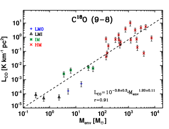
The values of the correlation coefficient and the fit parameters for all these molecular transitions are presented in Table 4. The correlation prevails for all transitions even if the values of integrated intensity are not converted to line luminosity. Therefore, () still correlates with () over at least 3 and 6 orders of magnitude on the y and x axis, respectively. Similar correlations are obtained when plotting the logarithm of versus the logarithm of the source envelope mass, , for all the targeted lines (see Fig. 7 for an example using the C18O =9–8 line). In these representations, the modelled envelope mass of the source is directly compared to , a tracer of the warm envelope mass. Therefore, the correlation is extended and probed by another proxy of the mass of the protostellar system.
Since the index of the fitted power-law exponents is 1 within the uncertainty of the fits (see Table 4), these correlations show that () is proportional to (). In the optically thin case, this correlation implies that the column density of warm CO increases proportionally with the mass of the young stellar object. This result can be applied to C18O because the emission lines of this isotopologue are expected to be optically thin. Assuming that 13CO =10–9 is optically thin as well, the column density would increase proportionally with the luminosity of the source, and practically with the same factor as the studied C18O transitions. Therefore, even though the conditions in low-, intermediate- and high-mass star-forming regions are different and distinct physical and chemical processes are expected to be more significant in each scenario (e.g., ionising radiation, clustering, etc.), the column density of CO seems to depend on the luminosity of the central protostar alone, showing a self-similar behaviour from low- to high-mass.
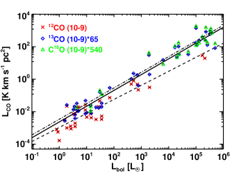
To test the optically thin assumption for 12CO =10–9 and especially for 13CO =10–9, the line luminosities for the 13CO =10–9 and the C18O =10–9 data were multiplied by a 12C/13C ratio of 65 (Vladilo et al. 1993)555 The 12C/13C ratio varies with galactocentric radius by up to a factor of 2 but this effect is minor and is ignored., and by a 16O/18O ratio of 540 (Wilson & Rood 1994), respectively. Therefore, the observed and predicted values of for 12CO =10–9 and 13CO =10–9, together with those of C18O =10–9 can be compared across the studied luminosity range (see Fig. 8). In the case of the 13CO =10–9 line, the values of the observed and predicted line luminosity are similar (20% in most of them), especially at lower luminosities. In addition, the slope of their fits are practically the same within the uncertainty, so a similar behaviour is proved. From these results we can assume that in general 13CO =10–9 is optically thin. For 12CO =10–9, the ratio of predicted to observed line luminosity (CO =10–9]/CO =10–9]) ranges from 0.8 to 12.5, for IRAS 15398 and W3-IRS5 respectively, and the average obtained is 3.3. Therefore, 12CO =10–9 is optically thick, at least at the line centre which dominates the intensity, and the relative value of the optical depth, , increases slightly with the mass of the protostar ( 1.5 for the low-mass sources, 2.0 for the intermediate and 3.4 for the high-mass object). This is in keeping with the expectation that massive YSOs form in the densest parts of the giant molecular clouds, GMCs.
Correcting for optical depth, CO =10–9] can be used to derive CO =10–9] because both species present a similar behaviour across the luminosity range (similar slopes in their fits). This relation can be used in the calculation of for those sources for which there are no 12CO =10–9 observations, that is, the high-mass sample. As highlighted before, using 13CO as a proxy for 12CO is restricted to comparisons of integrated intensities of the emission lines across the studied mass spectrum, and cannot be extended to the analysis of the line profile of 12CO and 13CO =10–9.

| Line | r | ||
|---|---|---|---|
| 12CO =10–9 | 2.9 0.2 | 0.84 0.06 | 0.92 |
| 13CO =10–9 | 4.4 0.2 | 0.97 0.03 | 0.98 |
| C18O =3–2 | 4.1 0.1 | 0.93 0.03 | 0.98 |
| C18O =5–4 | 3.5 0.2 | 0.78 0.08 | 0.93 |
| C18O =9–8 | 5.2 0.2 | 1.03 0.05 | 0.97 |
| C18O =10–9 | 5.2 0.3 | 0.96 0.06 | 0.96 |
3.3 Kinetic temperature
The ratio of the 12CO =10–9 and =3–2 line wings can be used to constrain the kinetic temperature of the entrained outflow gas if the two lines originate from the same gas. Yıldız et al. (2012) and (2013, submitted) have determined this for the sample of low-mass YSOs. Here we consider two sources to investigate whether the conditions in the outflowing gas change with increasing YSO mass: the intermediate-mass YSO NGC 2071 and the high-mass object W3-IRS5. The critical densities, , of the 12CO =3–2 and =10–9 transitions at 70 K are 2.0104 and 4.2105 cm-3, respectively. The values were calculated using equation 2 from Yang et al. (2010), the CO rate coefficients presented in their paper and considering only para-H2 collisions. The densities inside the HIFI beam for 12CO =10–9 (20) of both sources are higher than . Therefore, the emission is thermalised and can be directly constrained by the 12CO =10–9/=3–2 line wing ratios.
The observed ratios of the red and blue wings for these two sources as a function of absolute offset from the source velocity are presented in Fig. 9. These ratios are compared with the values calculated by Yıldız et al. (2013, submitted) from the 12CO =10–9 and =3–2 averaged spectra for the low-mass Class 0 sample (shaded regions). Since the emission is optically thin and we can assume LTE, the kinetic temperatures are calculated from the equation that relates the column density and the integrated intensity (Wilson et al. 2009). The obtained varies from 100 to 210 K. Both the observed line ratios as well as the inferred kinetic temperatures are similar to those found for the low-mass YSOs, where ranges from 70-200 K for Class 0. Although only a couple of higher-mass sources have been investigated, the temperatures in the entrained outflow gas seem to be similar across the mass range. Note that if part of the12CO =10–9 emission originates from a separate warmer component, the above values should be regarded as upper limits.
4 Discussion
The HIFI data show a variety of line profiles with spectra that can be decomposed into two different velocity components, such as the 12CO =10–9 lines, and spectra that show narrow single Gaussian profiles (C18O data). In addition, a strong correlation is found between the line and the bolometric luminosity for all lines. The next step is to analyse these results to better understand which physical processes are taking place.
Section 4.1 compares the narrow C18O lines and the 12CO broad velocity component in order to better understand the physics that these components are tracing and the regions of the protostellar environment they are probing. The dynamics of the inner envelope-outflow system is studied in Section 4.2. Finally, the interpretation of CO as a dense gas tracer is discussed in Section 4.3.
4.1 Broad and narrow velocity components
The broad velocity component identified in most of the 12CO =3–2 and =10–9 spectra is related to the velocity of the entrained outflowing material, so the wings of 12CO can be used as tracers of the outflow properties (Cabrit & Bertout 1992; Bachiller & Tafalla 1999). However, there are different effects that should be taken into account when this profile component is analysed, such as the viewing angle of the protostar and the S/N. The former could alter the width of the broad component due to projection or even make it disappear if the outflow is located in the plane of the sky. Low S/N could also hide the broad component for sources with weak emission. Moreover, the broad velocity component should be weaker if the emission lines come from sources at later evolutionary stages since their outflows become weaker and less collimated (see reviews of Bachiller & Tafalla 1999; Richer et al. 2000; Arce et al. 2007).
In order to compare the line profiles of all observed CO lines for each type of YSO and avoid the effects of inclination and observational noise playing a role in the global analysis of the data, an average spectrum of each line for each sub-type of protostar has been calculated and presented in Figs. 10 and 11. Regarding the low-mass sample, we observe a striking decrease in the width of the broad component from Class 0 to Class I. This result shows the decrease of the outflow force for more evolved sources in the low-mass sample is reflected in the average spectra (Bontemps et al. 1996).
A narrow velocity component has been defined as a line profile that can be fitted by a Gaussian function with a FWHM smaller than 7.5 km s-1 (see Section 2.4 for more details). Since C18O lines are expected to trace dense quiescent envelope material, high- transitions are probing the warm gas in the inner envelope. The average C18O spectra for each type of YSO are compared in Fig. 11. The FWHM of the emission lines increases from low- to high-mass protostars (see Fig. 5 and Table 3). An explanation for this result could be that for massive regions, the UV radiation from the forming OB star ionises the gas, creating an Hii region inside the envelope which increases the pressure on its outer envelope. This process may lead to an increase in the turbulent velocity of the envelope material (Matzner 2002), thus broadening the narrow component. Therefore, our spectra are consistent with the idea that in general, turbulence in the protostellar envelopes of high-mass objects is expected to be stronger than for low-mass YSOs (e.g. Herpin et al. 2012).
Higher rotational transitions trace material at higher temperatures and probe deeper and denser parts of the inner envelope. For the low- and intermediate-mass sources, the FWHM of the C18O =3–2 spectra are generally half that obtained for the C18O =9–8 and slightly smaller than those obtained for the =5–4 transition. However, for the high-mass YSOs the values of the FWHM are similar for the =3–2 and =9–8 transitions. In order to understand which kind of processes (thermal or non-thermal) dominate in the inner regions of the protostellar envelope traced by our observations, the contribution of these two processes to the line width is calculated. The aim is to explain whether the broadening of high- emission lines is caused by thermal or non-thermal motions.
In the case of the =3–2 lines, the upper energy level is 31 K, so the thermal line width, , is 0.12 km s-1 for C18O at this temperature. Comparing this value with the measured FWHM of the C18O =3–2 spectra in Table 10, we conclude that thermal motions contribute less than 5% to the total observed line width, . Therefore, the line width is dominated by non-thermal motions . The C18O =9–8 line profiles trace warmer gas (up to 300 K) with respect to =3–2 increasing the thermal contribution. However, even at 300 K is 0.68 km s-1, which means that is larger than 0.93 even for the low-mass sources. Thus, non-thermal motions predominate over thermal ones in the studied regions of the protostellar envelopes. These motions are assumed to be independent of scale and do not follow the traditional size-line width relation (Pineda et al. 2010). Therefore, these results are not biased by the distance of the source.
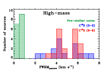
This analysis can be compared to pre-stellar cores, in which the line profiles are closer to being dominated by thermal motions. For this purpose, the line width values calculated for our data are compared to those of Jijina et al. (1999). In that work, a database of 264 dense cores mapped in the ammonia lines =(1,1) and (2,2) is presented. Histograms in Fig. 12 compare the values of the line widths observed for pre-stellar cores with the observed line width of the C18O =3–2 and =9–8 data for the WISH sample of protostars for low- (top) and for high-mass (bottom) objects. We observe that also for pre-stellar cores, the line widths are larger for more massive objects. From these histograms and following the previous discussion, we conclude that the broadening of the line profile from pre-stellar cores to protostars is due to non-thermal motions rather than thermal increase. Therefore, non-thermal processes (turbulence or infall motions) are crucial during the evolution of these objects and these motions increase with mass.

4.2 CO and dynamics: turbulence versus outflow
12CO and C18O spectra trace different physical structures originating close to the protostar (e.g. Yıldız et al. 2012). The broad wings of the 12CO =10–9 and =3–2 data are optically thin and trace fast-moving gas, that is, emission from entrained outflow material. On the other hand, the narrow C18O spectra probe the turbulent and infalling material in the protostellar envelope. The relationship between these two different components is still poorly understood.
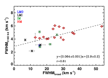
Following the discussion in 4.1, we compare the FWHM of the narrow component as traced by C18O =9–8 with the FWHM of the broad velocity component as traced by 12CO =10–9 or =3–2 for the sources detected in both transitions (see Fig. 13). The C18O =9–8 data were chosen for this comparison because this transition has been observed for the entire sample of YSOs, in contrast to C18O =5–4 and =10–9 transitions. A correlation is found (with a Pearson correlation coefficient 0.6), indicating a relationship between the fast outflowing gas and the quiescent envelope material.
Considering the scenario in which the non-thermal component is dominated by turbulence, the relation presented in Fig. 13 indicates that the increase of the velocity of the outflowing gas corresponds to an increase in the turbulence in the envelope material and this relation holds across the entire luminosity range. One option is that stronger outflows are injecting larger-scale movements into the envelope, which increases the turbulence. This effect is reflected as a broadening of the C18O line width. In addition, for the low-mass sources the width of the C18O =9–8 lines is larger than for the =3–2 spectra, indicating that the hotter inner regions of the envelope are more turbulent than its cooler outer parts. In the case of the high-mass object, the FWHMs of the C18O =9–8 and =3–2 lines are comparable, which could be partly caused because more luminous YSOs tend to be created in more massive and more turbulent molecular clouds (Wang et al. 2009).
Alternatively, infall processes could broaden the C18O profiles. Indeed, an increase in FWHM by at least 50% is found for C18O =9–8 compared with =3–2 in collapsing envelope simulations due to the higher infall velocities in the inner warm envelope (Harsono et al. 2013, submitted). If the non-thermal component was dominated by these movements, the sources with larger infall rates should have broader C18O line widths. These objects generally have larger outflow rates, i.e., higher outflow activity, (see Tomisaka 1998; Behrend & Maeder 2001) which shows up as a broadening of the 12CO wings since the amount of material injected into the outflow is larger. Therefore, we will observe the same result as in the previous scenario, that is, a broadening of the 12CO line wings for sources with stronger infalling motions. This relation would hold across the studied luminosity range.
Theoretically, large differences in the dynamics of the outflow-envelope system between low- and high-mass are expected since the same physical processes are not necessarily playing the same relevant roles in these different types of YSOs. However, Fig. 13 shows that the dynamics of the outflow and envelope are equally linked for the studied sample of protostars. With the current analysis we cannot disentangle which is the dominant motion in the non-thermal component of the line profile and thus, we cannot conclude if the infalling process makes the outflow stronger or if the outflow drives turbulence back into the envelope or a combined effect is at play.
4.3 High- CO as a dense gas tracer
The strictly linear relationships between CO high- line luminosity and bolometric luminosity presented in Figs. 6 to 8 require further discussion. The bolometric luminosity of embedded protostars is thought to be powered by accretion onto the growing star and is thus a measure of the mass accretion rate. A well-known relation of bolometric luminosity with the outflow momentum flux as measured from 12CO low- maps has been found across the stellar mass range (Lada & Fich 1995; Bontemps et al. 1996; Richer et al. 2000), so one natural explanation for our observed 12CO =10–9 correlation is that it reflects this same relation. However, the outflow wings contain only a fraction of the 12CO =10–9 emission, with the broad/narrow intensity ratios varying from source to source (Table 5, see also Yıldız et al. 2013, submitted, for the low-mass sources). Together with the fact that the relations hold equally well for 13CO and C18O high- lines, this suggests the presence of another underlying relation. Given the strong correlation with (Fig. 7), the most likely explanation is that the high- CO lines of all isotopologues trace primarily the amount of dense gas associated with the YSOs.
Can this relation be extended to larger scales than those probed here? Wu et al. (2005, 2010) found a linear relation between HCN integrated intensity and far-infrared luminosity for a set of galactic high-mass star forming regions on similar spatial scales as probed by our data. They have extended this relation to include extragalactic sources to show that this linear regime extends to the scales of entire galaxies, as first demonstrated by Gao & Solomon (2004). In contrast, the CO =1–0 line shows a superlinear relation with far-infrared luminosity (sometimes converted into star formation rate) and with the total (H I + H2) gas surface density with a power-law index of 1.4 (see Kennicutt & Evans 2012 for review). The data presented in this paper suggest that it is the mass of dense molecular gas as traced by HCN that controls the relation on large scales rather than the mass traced by CO =1–0 (see also Lada et al. 2012).
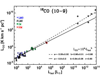
With the increased number of detections of 12CO =10–9 in local and high redshift galaxies with Herschel (e.g., van der Werf et al. 2010; Spinoglio et al. 2012; Kamenetzky et al. 2012; Meijerink et al. 2013) and millimeter interferometers (e.g., Wei et al. 2007; Scott et al. 2011), the question arises whether this line can serve as an equally good tracer of dense gas. As an initial test, we present in Fig. 14 our 12CO =10–9 - (assuming ) relation with these recent extragalactic detections included. As can be seen, the relation does indeed extend to larger scales. Given the small number statistics, the correlation has only limited meaning and this relation needs to be confirmed by additional data.
An alternative view has been presented by Krumholz & Thompson (2007) and Narayanan et al. (2008) who argue that the linearity for dense gas tracers is a coincidence resulting from the fact that these higher excitation lines are subthermally excited and probe only a small fraction of the total gas. They suggest that the relation should change with higher critical density tracers and even become sublinear with a power-law index less than 0.5 for transitions higher than =7–6 for CO. On the small scales probed by our data, we do not see this effect and the linear relations clearly continue to hold up to the =10–9 transition.
5 Conclusions
The analysis of the 12CO =3–2, =10–9, 13CO =10–9, C18O =3–2, =5–4, =9–8 and =10–9 line profiles allows us to study several fundamental parameters of the emission line, such as the line width and the line luminosity, and to constrain the dynamics of different physical structures of WISH protostars across a wide range of luminosities. Complementing the HIFI data, lower- observations from the JCMT are included in order to achieve a uniform picture of the interaction of YSOs with their immediate surroundings. Our results are summarised as follows:
-
A gallery of line profiles identified in the HIFI CO spectra is presented. 12CO and 13CO =10–9 line profiles can be decomposed into two different velocity components, where the broader component is thought to trace the entrained outflowing gas. This broad component weakens from the low-mass Class 0 to Class I stage. Meanwhile, the narrow C18O lines probe the bulk of the quiescent envelope material. The widths are dominated by non-thermal motions including turbulence and infall. The next step will be to constrain the contribution of these non-thermal mechanisms on the C18O line profiles by using radiative transfer codes such as RATRAN (Hogerheijde & van der Tak 2000).
-
The narrow C18O =9–8 line widths increase from low- to high-mass YSOs. Moreover, for low- and intermediate-mass protostars, they are about twice the width of the C18O =3–2 lines, suggesting increased turbulence/faster infall in the warmer inner envelope compared to the cooler outer envelope. For high-mass objects the widths of the =9–8 and =3–2 lines are comparable, suggesting that the molecular clouds in which these luminous YSOs form are more turbulent. Extending the line width analysis to pre-stellar cores, a broadening of the line profile is observed from these objects to protostars caused by non-thermal processes.
-
A correlation is found between the width of the 12CO =3–2 and =10–9 broad velocity component and the width of the C18O =9–8 profile. This suggests a link between entrained outflowing gas and envelope motions (turbulence and/or infalling) which holds from low- to high-mass YSOs. This means that the interaction and effect of outflowing gas and envelope material is the same across the studied luminosity range, indicative of the existence of an underlying common physical mechanism which is independent of the source mass.
-
A strong linear correlation is found between the logarithm of the line and bolometric luminosities across six orders of magnitude on both axes, for all lines and isotopologues. This correlation is also found between the logarithm of the line luminosity and envelope mass. This indicates that high- CO transitions (up to =10–9) can be used as a dense gas tracer, a relation that can be extended to larger scales (local and high redshift galaxies).
Acknowledgements.
The authors are grateful to the external referee Andrés Guzmán for his careful and detailed report and to the editor Malcom Walmsley for his useful last comments. These two reports helped to improve considerably this manuscript. We would also like to thank the WISH team for many inspiring discussions, in particular the WISH internal referees Gina Santangelo and Luis Chavarría. Astrochemistry in Leiden is supported by the Netherlands Research School for Astronomy (NOVA), by a Spinoza grant and grant 614.001.008 from the Netherlands Organisation for Scientific Research (NWO), and by the European Community’s Seventh Framework Programme FP7/2007-2013 under grant agreement 238258 (LASSIE). We would like to thanks the JCMT, which is operated by The Joint Astronomy Centre on Behalf of the Science and Technology Facilities Council of the United Kingdom, the Netherlands Organisation for Scientific Research, and the National Research Council of Canada. This research used the facilities of the Canadian Astronomy Data Centre operated by the National Research Council of Canada with support of the Canadian Space agency. HIFI has been designed and built by a consortium of institutes and university departments from across Europe, Canada and the United States under the leadership of SRON Netherlands Institute for Space Research, Groningen, The Netherlands and with major contributions from Germany, France and the US. Consortium members are: Canada: CSA, U.Waterloo; France: CESR, LAB, LERMA, IRAM; Germany: KOSMA, MPIfR, MPS; Ireland, NUI Maynooth; Italy: ASI, IFSI-INAF, Osservatorio Astrofisico di Arcetri- INAF; Netherlands: SRON, TUD; Poland: CAMK, CBK; Spain: Observatorio Astronómico Nacional (IGN), Centro de Astrobiología (CSIC-INTA). Sweden: Chalmers University of Technology - MC2, RSS GARD; Onsala Space Observatory; Swedish National Space Board, Stockholm University - Stockholm Observatory; Switzerland: ETH Zurich, FHNW; USA: Caltech, JPL, NHSC.References
- Arce et al. (2007) Arce, H. G., Shepherd, D., Gueth, F., et al. 2007, Protostars and Planets V, 245
- Bachiller et al. (1990) Bachiller, R., Martín-Pintado, J., Tafalla, M., Cernicharo, J., & Lazareff, B. 1990, A&A, 231, 174
- Bachiller & Tafalla (1999) Bachiller, R., & Tafalla, M. 1999, in The Origin of Stars and Planetary Systems, eds. Lada, C. J. & Kylafis, N. D. (Kluwer: Dordrecht), p. 227
- Behrend & Maeder (2001) Behrend, R., & Maeder, A. 2001, A&A, 373, 190
- Beuther et al. (2002) Beuther, H., Schilke, P., Sridharan, T. K., et al. 2002, A&A, 383, 892
- Beuther & Shepherd (2005) Beuther, H., & Shepherd, D. 2005, Cores to Clusters: Star Formation with Next Generation Telescopes, 105
- Bontemps et al. (1996) Bontemps, S., André, P., Terebey, S., & Cabrit, S. 1996, A&A, 311, 858
- Buckle et al. (2009) Buckle, J. V., Hills, R. E., Smith, H., et al. 2009, MNRAS, 399, 1026
- Cabrit & Bertout (1992) Cabrit, S., & Bertout, C. 1992, A&A, 261, 274
- Cesaroni (2005) Cesaroni, R. 2005, Massive Star Birth: A Crossroads of Astrophysics, 227, 59
- Churchwell (1999) Churchwell, E. 1999, in The Origin of Stars and Planetary Systems, eds. Lada, C. J. & Kylafis, N. D. (Kluwer: Dordrecht), p. 515
- Curtis et al. (2010) Curtis, E. I., Richer, J. S., Swift, J. J., & Williams, J. P. 2010, MNRAS, 408, 1516
- van Dishoeck & Blake (1998) van Dishoeck, E. F., & Blake, G. A. 1998, ARA&A, 36, 317
- van Dishoeck et al. (2011) van Dishoeck, E. F., Kristensen, L. E., Benz, A. O., et al. 2011, PASP, 123, 138
- Evans (1999) Evans, N. J., II 1999, ARA&A, 37, 311
- Evans et al. (2009) Evans, N., Calvet, N., Cieza, L., et al. 2009, arXiv:0901.1691
- Fuller & Ladd (2002) Fuller, G. A., & Ladd, E. F. 2002, ApJ, 573, 699
- Gao & Solomon (2004) Gao, Y., & Solomon, P. M. 2004, ApJS, 152, 63
- de Graauw et al. (2010) de Graauw, T., Helmich, F. P., Phillips, T. G., et al. 2010, A&A, 518, L6
- Graves et al. (2010) Graves, S. F., Richer, J. S., Buckle, J. V., et al. 2010, MNRAS, 409, 1412
- Harsono et al. (2013, submitted) Harsono, D., Visser, R., Bruderer, S., van Dishoeck, E. F., Kristensen, L. E., et al. 2013, submitted, A&A
- Herpin et al. (2012) Herpin, F., Chavarría, L., van der Tak, F., et al. 2012, A&A, 542, A76
- Hogerheijde & van der Tak (2000) Hogerheijde, M. R., & van der Tak, F. F. S. 2000, A&A, 362, 697
- Hollenbach & Tielens (1999) Hollenbach, D. J., & Tielens, A. G. G. M. 1999, Reviews of Modern Physics, 71, 173
- Jijina & Adams (1996) Jijina, J., & Adams, F. C. 1996, ApJ, 462, 874
- Jijina et al. (1999) Jijina, J., Myers, P. C., & Adams, F. C. 1999, ApJS, 125, 161
- Jørgensen et al. (2002) Jørgensen, J. K., Schöier, F. L., & van Dishoeck, E. F. 2002, A&A, 389, 908
- Kamenetzky et al. (2012) Kamenetzky, J., Glenn, J., Rangwala, N., et al. 2012, ApJ, 753, 70
- Kennicutt & Evans (2012) Kennicutt, R. C., Jr, & Evans, N. J., 2012, ARA&A, 50, 531
- Kristensen et al. (2010) Kristensen, L. E., Visser, R., van Dishoeck, E. F., et al. 2010, A&A, 521, L30
- Kristensen et al. (2011) Kristensen, L. E., van Dishoeck, E. F., Tafalla, M., et al. 2011, A&A, 531, L1
- Kristensen et al. (2012) Kristensen, L. E., van Dishoeck, E. F., Bergin, E. A., et al. 2012, A&A, 542, A8
- Krumholz & Thompson (2007) Krumholz, M. R., & Thompson, T. A. 2007, ApJ, 669, 289
- Lacy et al. (1994) Lacy, J. H., Knacke, R., Geballe, T. R., & Tokunaga, A. T. 1994, ApJ, 428, L69
- Lada & Fich (1995) Lada, C. J., & Fich, M. 1995, Revista Mexicana de Astronomia y Astrofisica Conference Series, 1, 93
- Lada (1999) Lada, C. J. 1999, in The Origin of Stars and Planetary Systems, eds. Lada, C. J. & Kylafis, N. D. (Kluwer: Dordrecht), p.143
- Lada et al. (2012) Lada, C. J., Forbrich, J., Lombardi, M., & Alves, J. F. 2012, ApJ, 745, 190
- Matzner (2002) Matzner, C. D. 2002, ApJ, 566, 302
- McCoey et al. (in prep.) McCoey, C. et al. 2013, in prep.
- Meijerink et al. (2013) Meijerink, R., Kristensen, L. E., Weiß, A., et al. 2013, ApJ, 762, L16
- McKee & Ostriker (2007) McKee, C. F., & Ostriker, E. C. 2007, ARA&A, 45, 565
- Mottram et al. (2011) Mottram, J. C., Hoare, M. G., Davies, B., et al. 2011, ApJ, 730, L33
- Narayanan et al. (2008) Narayanan, D., Cox, T. J., Shirley, Y., et al. 2008, ApJ, 684, 996
- Ott (2010) Ott, S. 2010, ASP Conf. Series, 434, 139
- Palla & Stahler (1993) Palla, F., & Stahler, S. W. 1993, ApJ, 418, 414
- Pilbratt et al. (2010) Pilbratt, G. L., Riedinger, J. R., Passvogel, T., et al. 2010, A&A, 518, L1
- Pineda et al. (2010) Pineda, J. E., Goodman, A. A., Arce, H. G., et al. 2010, ApJ, 712, L116
- Plume et al. (2012) Plume, R., Bergin, E. A., Phillips, T. G., et al. 2012, ApJ, 744, 28
- Richer et al. (2000) Richer, J. S., Shepherd, D. S., Cabrit, S., Bachiller, R., & Churchwell, E. 2000, Protostars and Planets IV, 867
- Roelfsema et al. (2012) Roelfsema, P. R., Helmich, F. P., Teyssier, D., et al. 2012, A&A, 537, A17
- Santangelo et al. (2012) Santangelo, G., Nisini, B., Giannini, T., et al. 2012, A&A, 538, A45
- Scott et al. (2011) Scott, K. S., Lupu, R. E., Aguirre, J. E., et al. 2011, ApJ, 733, 29
- Shepherd & Churchwell (1996) Shepherd, D. S., & Churchwell, E. 1996, ApJ, 472, 225
- Shu (1977) Shu, F. H. 1977, ApJ, 214, 488
- Shu et al. (1993) Shu, F., Najita, J., Galli, D., Ostriker, E., & Lizano, S. 1993, Protostars and Planets III, 3
- Spaans et al. (1995) Spaans, M., Hogerheijde, M. R., Mundy, L. G., & van Dishoeck, E. F. 1995, ApJ, 455, L167
- Spinoglio et al. (2012) Spinoglio, L., Pereira-Santaella, M., Busquet, G., et al. 2012, ApJ, 758, 108
- van der Tak et al. (2013, submitted) van der Tak, F. F. S., Chavarría, L., Herpin, F. et al. 2013, submitted, A&A
- Tomisaka (1998) Tomisaka, K. 1998, ApJ, 502, L163
- Vasta et al. (2012) Vasta, M., Codella, C., Lorenzani, A., et al. 2012, A&A, 537, A98
- Vladilo et al. (1993) Vladilo, G., Centurion, M., & Cassola, C. 1993, A&A, 273, 239
- Wampfler et al. (2013, in press) Wampfler, S. F., Bruderer, S., Karska, A. et al. 2013, in press, A&A
- Wang et al. (2009) Wang, K., Wu, Y. F., Ran, L., Yu, W. T., & Miller, M. 2009, A&A, 507, 369
- Wei et al. (2007) Wei, A., Downes, D., Neri, R., et al. 2007, A&A, 467, 955
- van der Werf et al. (2010) van der Werf, P. P., Isaak, K. G., Meijerink, R., et al. 2010, A&A, 518, L42
- van der Wiel et al. (2013, submitted) van der Wiel, M. H. D., Pagani, L., van der Tak, F. F. S., Doty, C. D. et al. 2013, submitted, A&A
- Wilson & Rood (1994) Wilson, T. L., & Rood, R. 1994, ARA&A, 32, 191
- Wilson et al. (2009) Wilson, T. L., Rohlfs, K., Hüttemeister, S. 2009, Tools of Radio Astronomy (Springer-Verlag: Berlin)
- Wu et al. (2005) Wu, J., Evans, N. J., II, Gao, Y., et al. 2005, ApJ, 635, L173
- Wu et al. (2010) Wu, J., Evans, N. J., II, Shirley, Y. L., & Knez, C. 2010, ApJS, 188, 313
- Wyrowski et al. (2010) Wyrowski, F., van der Tak, F., Herpin, F., et al. 2010, A&A, 521, L34
- Yang et al. (2010) Yang, B., Stancil, P. C., Balakrishnan, N., & Forrey, R. C. 2010, ApJ, 718, 1062
- Yıldız et al. (2010) Yıldız, U. A., van Dishoeck, E. F., Kristensen, L. E., et al. 2010, A&A, 521, L40
- Yıldız et al. (2012) Yıldız, U. A., Kristensen, L. E., van Dishoeck, E. F., et al. 2012, A&A, 542, A86
- Yıldız et al. (2013, submitted) Yıldız, U. A., Kristensen, L. E., van Dishoeck, E. F., San José-García, I. et al. 2013, submitted, A&A
Appendix A Characterisation of the HIFI data
The main characteristics of the HIFI data, together with the spectra are presented in this appendix. The description of the observed lines focuses first on 12CO =10–9 (Section A.1), where the main characteristics for the low-, intermediate- and high-mass sources are listed in this order. Next we discuss the 13CO =10–9 spectra (Section A.2), following the same structure, and finally all observed C18O lines (Section A.3) are presented.
A.1 12CO =10–9 line profiles
The 12CO =10–9 line was observed for the entire sample of low- and intermediate-mass YSOs and for one high-mass object (W3-IRS5). All the observed sources were detected and the emission profiles are the strongest and broadest among the targeted HIFI CO lines (see Fig. 15 and Table 5 for further information). Within the low-mass Class 0 sample, the main beam peak temperature, , ranges from 0.8 to 8.1 K. As indicated in Section 2.4, the emission in some sources (around 73 % of the detected lines of this sub-group) can be decomposed into two velocity components. The FWHM of the narrower component varies from 2.3 km s-1 to 9.3 km s-1, while the width of the broad component shows a larger variation, from 8.3 km s-1 to 41.0 km s-1. For the low-mass Class I YSOs, similar intensity ranges are found, with varying from 0.6 to 10.2 K. The Class I protostars present narrower emission lines than the Class 0 sources and only the 27 % of the emission line profiles can be decomposed into two velocity components. The narrow component ranges from 1.8 to 5.1 km s-1 and the broad component varies from 10.0 to 16.1 km s-1.
For the intermediate-mass protostars, the intensity increases and varies from =2.4 to 28.0 K. The profiles are broader and the distinction between the two different components is clearer than for the low-mass sources, so all profiles can be fitted with two Gaussian functions. The FWHM of the two identified velocity components varies from 2.7 to 7.6 km s-1 for the narrow component and from 15.6 to 24.3 km s-1 for the broad component.
Only W3-IRS5 was observed in 12CO =10–9 from the high-mass sample. The spectrum is presented in Appendix B, Fig. 22, together with other lines of this source. The profile is more intense than any of the low- and intermediate-mass sources (=48.5 K) and has the largest FWHM: 8.4 km s-1 for the narrower component and 28.6 km s-1 for the broad component.
Self-absorption features have been detected in 5 out of 33 observed 12CO =10–9 emission lines (the sources are indicated in Table 5). However, these features are weak and of the order of the rms of the spectrum, so no Gaussian profile has been fitted. No specific symmetry can be determined, that is, there is no systematic shift in the emission of the broad component relative to the source velocity (see Fig. 15 for comparison). Overall, the data do not show any infall signature.
| Source | rmsa | |||||||
|---|---|---|---|---|---|---|---|---|
| (mK) | (K km s-1) | (K) | (K) | (km s-1) | (km s-1) | (km s-1) | (km s-1) | |
| Low-mass: Class 0 | ||||||||
| L 1448-MMd | 91 | 21.5 | 0.4 | 0.9 | 10.3 | 6.0 | 41.0 | 4.8 |
| NGC 1333 IRAS 2A | 104 | 20.3 | 0.4 | 1.5 | 12.8 | 8.2 | 8.3 | 3.9 |
| NGC 1333 IRAS 4Ac | 105 | 45.5 | 1.8 | 10.3 | 24.8 | |||
| NGC 1333 IRAS 4B | 104 | 32.4 | 1.4 | 1.5 | 8.1 | 7.1 | 16.5 | 3.3 |
| L 1527c | 93 | 4.8 | 1.6 | 4.9 | 2.4 | |||
| Ced110 IRS4c | 127 | 4.9 | 1.6 | 4.2 | 2.5 | |||
| IRAS 15398 | 132 | 16.5 | 0.5 | 2.5 | 1.0 | 4.1 | 15.0 | 4.2 |
| BHR 71de | 111 | 9.9 | 0.2 | 0.6 | 8.5 | 5.4 | 30.8 | 9.3 |
| L 483-MM | 108 | 10.9 | 0.3 | 1.5 | 2.8 | 5.3 | 19.1 | 2.9 |
| Ser SMM 1e | 98 | 81.3 | 3.4 | 4.1 | 7.1 | 8.6 | 15.6 | 5.9 |
| Ser SMM 3 | 102 | 33.7 | 1.0 | 2.0 | 8.8 | 7.0 | 20.8 | 4.1 |
| Ser SMM 4 | 97 | 39.0 | 1.6 | 3.3 | 2.1 | 6.8 | 10.7 | 4.3 |
| L 723-MMc | 110 | 6.8 | 1.1 | 10.9 | 4.9 | |||
| B335 | 120 | 11.1 | 0.5 | 1.0 | 8.9 | 8.3 | 16.1 | 2.3 |
| L 1157 | 103 | 9.5 | 0.3 | 0.5 | 0.4 | 2.9 | 26.8 | 2.7 |
| Low-mass: Class I | ||||||||
| L 1489c | 123 | 5.8 | 0.9 | 7.0 | 4.9 | |||
| L 1551 IRS 5 | 113 | 15.9 | 0.4 | 3.1 | 4.2 | 6.2 | 16.1 | 2.5 |
| TMR 1 c | 113 | 9.3 | 1.8 | 5.5 | 3.9 | |||
| TMC 1Ac | 137 | 4.2 | 0.5 | 5.7 | 3.6 | |||
| TMC 1c | 119 | 2.7 | 0.4 | 5.2 | 4.4 | |||
| HH 46 | 127 | 9.5 | 0.4 | 1.7 | 6.0 | 5.6 | 12.7 | 1.8 |
| IRAS 12496c | 100 | 10.0 | 2.1 | 2.8 | 3.8 | |||
| GSS 30 IRS1e | 127 | 44.6 | 1.1 | 8.0 | 2.9 | 2.7 | 10.0 | 3.7 |
| Elias 29c | 120 | 47.0 | 7.8 | 4.2 | 5.1 | |||
| Oph IRS 63c | 124 | 1.0 | 0.5 | 2.6 | 2.1 | |||
| RNO 91c | 114 | 7.6 | 1.5 | 0.4 | 2.4 | |||
| Intermediate-mass | ||||||||
| L1641 S3 MMS1 | 100 | 31.4 | 0.8 | 1.4 | 5.5 | 5.3 | 21.1 | 7.0 |
| Vela IRS 19 | 110 | 42.2 | 1.3 | 2.1 | 14.9 | 11.5 | 22.0 | 3.3 |
| Vela IRS 17 | 107 | 94.0 | 1.9 | 11.3 | 5.6 | 3.9 | 15.8 | 4.6 |
| NGC 7129 FIRS 2e | 100 | 29.8 | 0.9 | 1.2 | 11.5 | 8.9 | 20.9 | 5.1 |
| NGC 2071 | 162 | 421.6 | 7.0 | 13.9 | 8.2 | 10.9 | 24.3 | 7.6 |
| AFGL 490 | 129 | 29.6 | 1.2 | 3.0 | 11.5 | 13.4 | 15.6 | 2.7 |
| High-mass | ||||||||
| W3IRS5e | 102 | 674.8 | 10.8 | 32.0 | 40.7 | 37.5 | 28.6 | 8.4 |
Notes. (a) In 0.27 km s-1 bins.
(b) Integrated over the entire line, not including “bullet” emission.
(c) Single Gaussian fit. (d) EHV emission features
removed from the spectra by using two additional Gaussian fit
profiles. (e) Self-absorption features detected.
A.2 13CO =10–9 line profiles
The observed 13CO =10–9 emission lines for the low- and intermediate-mass sources are less intense, narrower and have a lower S/N than the 12CO =10–9 spectra (Fig. 16). Table 6 contains the parameters obtained from the one or two Gaussian fit to the detected line profiles. In the case of the low-mass Class 0 spectra, three sources are not detected down to 17 mK rms in 0.27 km s-1 bins and the profile of only two sources (Ser SMM1 and NGC1333 IRAS4A) can be decomposed into two different velocity components. The ranges from 0.05 to 0.8 K and the FWHM of the narrow profiles varies from 0.7 to 6.8 km s-1, with the largest values corresponding to the broad velocity component being 13.2 km s-1 for NGC1333 IRAS4A. In the case of the Class I sample, four sources are not detected and none of the emission line profiles can be decomposed into two velocity components. The averaged intensity is lower than for the Class 0 objects, ranging from =0.05 to 0.52 K. The value of the line width also drops and the interval varies from 1.5 to 7.3 km s-1.
For the intermediate-mass YSOs, a better characterisation of the line profile is possible since the lines are stronger and have higher S/N than the low-mass objects with ranging from 0.1 to 2.7 K. Compared to the 12CO =10–9 profiles, the 13CO =10–9 lines are more symmetric and only the emission profile of one source can be decomposed into two different Gaussian components. Regarding the FWHM of the lines fitted by the narrow Gaussian, the interval goes from 4.3 to 6.1 km s-1.
Around 63 of the detected 13CO =10–9 emission lines (12 out of 19) for the high-mass YSOs can be decomposed into two distinct velocity components, whereas the decomposition of the profiles is only possible for 10% of the detected low-mass objects (2 out of 20) and for 17% of the detected intermediate-mass YSOs (1 out of 6). The reason for the lower percentage recorded for the low- and intermediate-mass sources could be caused by a lower S/N compared with the bright high-mass sources. The weakest line from the high-mass sample has a of 0.7 K and the most intense a of 20.8 K. The FWHM of the narrower component varies from 3.3 km s-1 to 7.2 km s-1. The width of the broad component presents a larger variation since the minimum value is 8.7 km s-1 and the maximum 21.9 km s-1. This component appears either red- or blue-shifted. There is no significant trend with evolution stage as probed by the presence of IR-brightness or ionising radiation (Fig. 16).
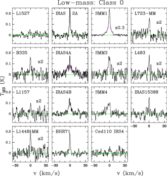
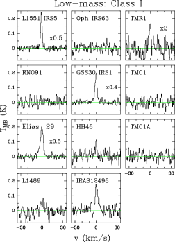
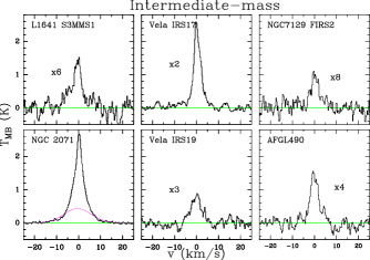
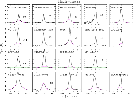
| Source | rmsa | |||||||
|---|---|---|---|---|---|---|---|---|
| (mK) | (K km s-1) | (K) | (K) | (km s-1) | (km s-1) | (km s-1) | (km s-1) | |
| Low-mass: Class 0 | ||||||||
| L 1448-MM | 20 | 0.2 | 0.1 | 4.7 | 1.6 | |||
| NGC 1333 IRAS 2A | 15 | 0.8 | 0.2 | 7.5 | 2.1 | |||
| NGC 1333 IRAS 4A | 23 | 1.1 | 0.07 | 0.09 | 5.7 | 6.7 | 13.2 | 0.7 |
| NGC 1333 IRAS 4B | 17 | 0.8 | 0.1 | 6.9 | 6.8 | |||
| IRAS 15398 | 24 | 0.2 | 0.16 | 5.0 | 1.1 | |||
| BHR 71 | 17 | 0.4 | 0.2 | –4.6 | 1.8 | |||
| L 483-MM | 16 | 0.3 | 0.1 | 5.0 | 2.4 | |||
| Ser SMM 1 | 22 | 4.0 | 0.2 | 0.5 | 7.6 | 8.3 | 10.6 | 2.4 |
| Ser SMM 3 | 20 | 0.3 | 0.1 | 7.2 | 4.0 | |||
| Ser SMM 4 | 25 | 0.6 | 0.1 | 5.7 | 6.0 | |||
| L 723-MM | 16 | 0.3 | 0.1 | 11.5 | 2.7 | |||
| B335 | 20 | 0.3 | 0.1 | 8.1 | 2.3 | |||
| L 1157 | 20 | 0.1 | 0.05 | 3.0 | 2.2 | |||
| Low-mass: Class I | ||||||||
| L 1489 | 32 | 0.4 | 0.05 | 7.8 | 7.3 | |||
| L 1551 IRS 5 | 29 | 1.3 | 0.47 | 6.5 | 2.4 | |||
| TMR 1 | 29 | 0.3 | 0.08 | 6.0 | 3.6 | |||
| HH 46 | 30 | 0.1 | 0.11 | 5.4 | 1.5 | |||
| IRAS 12496 | 28 | 0.8 | 0.15 | 3.1 | 4.2 | |||
| GSS 30 IRS1 | 33 | 2.0 | 0.46 | 2.8 | 3.4 | |||
| Elias 29 | 28 | 2.1 | 0.38 | 4.7 | 5.1 | |||
| Intermediate-mass | ||||||||
| L1641 S3 MMS1 | 38 | 1.8 | 0.2 | 4.7 | 6.1 | |||
| Vela IRS 19 | 41 | 1.1 | 0.2 | 12.1 | 5.9 | |||
| Vela IRS 17 | 43 | 4.9 | 0.8 | 0.4 | 4.4 | |||
| NGC 7129 FIRS 2 | 20 | 0.9 | 0.1 | –9.6 | 4.3 | |||
| NGC 2071 | 17 | 16.6 | 0.4 | 2.1 | 9.1 | 9.8 | 14.7 | 4.7 |
| AFGL 490 | 47 | 2.6 | 0.3 | –13.5 | 4.8 | |||
| High-mass | ||||||||
| IRAS05358+3543 | 18 | 6.2 | 0.2 | 0.7 | –15.1 | –15.9 | 15.4 | 3.7 |
| IRAS162724837 | 18 | 3.9 | 0.7 | –47.0 | 4.8 | |||
| NGC6334-I(N) | 23 | 13.8 | 0.5 | 1.3 | –5.7 | –3.8 | 13.3 | 4.4 |
| W43-MM1 | 38 | 4.5 | 0.8 | 98.4 | 5.8 | |||
| DR21(OH) | 18 | 52.2 | 0.9 | 5.7 | –1.9 | –3.3 | 16.0 | 5.8 |
| W3-IRS5 | 21 | 129.6 | 2.1 | 17.0 | –38.7 | –38.3 | 14.7 | 4.7 |
| IRAS180891732 | 27 | 8.3 | 1.4 | 33.0 | 4.6 | |||
| W33A | 19 | 11.4 | 0.5 | 1.1 | 36.8 | 37.7 | 11.7 | 3.5 |
| IRAS181511208 | 19 | 3.4 | 0.8 | 33.4 | 3.6 | |||
| AFGL2591 | 19 | 29.5 | 0.8 | 5.4 | –5.8 | –5.4 | 9.8 | 3.3 |
| G3270.6 | 25 | 12.8 | 1.8 | –44.8 | 6.6 | |||
| NGC6334-I | 23 | 57.7 | 0.7 | 7.2 | –6.7 | –6.8 | 17.8 | 5.4 |
| G29.960.02 | 46 | 31.3 | 0.6 | 4.6 | 96.9 | 98.8 | 13.6 | 4.6 |
| G31.41+0.31 | 52 | 17.4 | 2.5 | 96.8 | 6.1 | |||
| G5.890.39 | 34 | 133.7 | 2.6 | 6.2 | 10.5 | 9.4 | 21.9 | 5.9 |
| G10.47+0.03 | 200 | 26.2 | 1.8 | 66.8 | 10.0 | |||
| G34.26+0.15 | 59 | 58.8 | 1.3 | 6.7 | 58.0 | 57.7 | 12.0 | 5.0 |
| W51N-e1 | 50 | 70.2 | 1.3 | 5.0 | 58.6 | 57.1 | 18.6 | 7.2 |
| NGC7538-IRS1 | 24 | 41.0 | 2.0 | 5.3 | –59.8 | –57.6 | 8.7 | 3.5 |
Notes. (a) In 0.27 km s-1 bins.
(b) Integrated over the entire line.
A.3 C18O line profiles
Three transitions of C18O were obtained within WISH together with water observations: C18O =5–4, =9–8 and =10–9. Only Class 0 and intermediate-mass YSOs were observed in C18O =5–4, tracing regions with an upper energy level of 79 K (see Fig. 17). This line is obtained in parallel with a deep integration on the 548 GHz HO transition for 19 sources. Thus, the spectra have very high S/N with an rms of 9 mK for low-mass Class 0 sources and less than 20 mK for intermediate-mass YSOs in 0.27 km s-1 bins. The main characteristic of this transition is the narrow profile seen in all the emission lines for the narrower component, with a FWHM of less than 2.0 km s-1 for the low-mass sources, and 3.7 km s-1 for the intermediate-mass objects. In addition, other features are detected thanks to the high S/N, e.g. a weak broad velocity component for the low-mass objects NGC1333 IRAS 4A (Yıldız et al. 2010), L483, Ser SMM1 and Ser SMM4. This component is also identified in the C18O =5–4 line for the intermediate-mass sources NGC2071 (see Fig. 3) and Vela IRS19. The values of the single or two Gaussian fit of these lines are presented in Table 7.
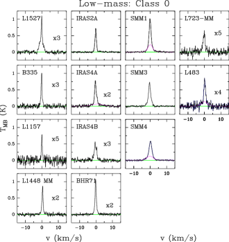

| Source | rmsa | |||||||
|---|---|---|---|---|---|---|---|---|
| (mK) | (K km s-1) | (K) | (K) | (km s-1) | (km s-1) | (km s-1) | (km s-1) | |
| Low-mass: Class 0 | ||||||||
| L 1448-MM | 4 | 0.47 | 0.37 | 5.1 | 1.3 | |||
| NGC 1333 IRAS 2A | 2 | 0.87 | 0.52 | 7.5 | 1.4 | |||
| NGC 1333 IRAS 4A | 4 | 0.68 | 0.03 | 0.32 | 7.9 | 6.9 | 7.8 | 1.3 |
| NGC 1333 IRAS 4B | 3 | 0.32 | 0.14 | 7.0 | 1.9 | |||
| L 1527 | 3 | 0.55 | 0.23 | 5.7 | 2.0 | |||
| BHR 71 | 3 | 0.63 | 0.37 | –4.7 | 1.4 | |||
| L 483-MM | 3 | 0.31 | 0.03 | 0.16 | 5.2 | 5.4 | 4.3 | 1.1 |
| Ser SMM 1 | 4 | 1.93 | 0.13 | 0.84 | 8.7 | 8.4 | 4.2 | 1.4 |
| Ser SMM 3 | 5 | 1.40 | 0.55 | 7.6 | 2.0 | |||
| Ser SMM 4 | 3 | 1.55 | 0.13 | 0.44 | 7.6 | 7.7 | 4.7 | 1.8 |
| L 723-MM | 5 | 0.19 | 0.09 | 10.0 | 1.9 | |||
| B335 | 4 | 0.26 | 0.22 | 8.2 | 1.2 | |||
| L 1157 | 4 | 0.15 | 0.09 | 2.6 | 1.3 | |||
| Intermediate-mass | ||||||||
| L1641 S3 MMS1 | 20 | 0.73 | 0.40 | 5.2 | 1.7 | |||
| Vela IRS 19 | 10 | 1.67 | 0.05 | 0.46 | 12.5 | 11.6 | 9.2 | 2.4 |
| Vela IRS 17 | 25 | 5.32 | 1.25 | 4.1 | 3.7 | |||
| NGC 7129 FIRS 2 | 4 | 0.55 | 0.18 | –9.9 | 2.3 | |||
| NGC 2071 | 5 | 7.29 | 0.55 | 1.33 | 8.9 | 9.6 | 7.4 | 2.0 |
| AFGL 490 | 14 | 3.55 | 1.04 | –13.3 | 2.7 |
Notes. (a) In 0.27 km s-1 bins.
(b) Integrated over the entire line.
For the =9–8 transition, 55% of the observed lines are detected, probably due to the lower caused by shorter exposure times than for the =5–4 line. The lines are detected in 5 out of 26 low-mass sources; 4 out of 6 intermediate-mass YSOs; and in all 19 high-mass protostars (see Fig. 18). The C18O =9–8 emission lines appear weak with median values of 0.10, 0.14 and 0.83 K for the low-, intermediate- and high-mass objects, respectively. Most of the emission line profiles of C18O =9–8 can be fitted by a single Gaussian with a FWHM from 2.0 km s-1 to 3.9 km s-1 for the low-mass objects; from 2.8 km s-1 to 5.4 km s-1 for the intermediate-mass sources; and from 3.1 to 6.4 km s-1 for the high-mass YSOs (values summarised in Table 8). Only a two Gaussian decomposition has been performed for three ultra-compact HII regions (G10.47+0.03, W51N-e1 and G5.89-0.39). For these objects, the broad velocity components are larger than 16 km s-1, as is shown in Fig. 18.
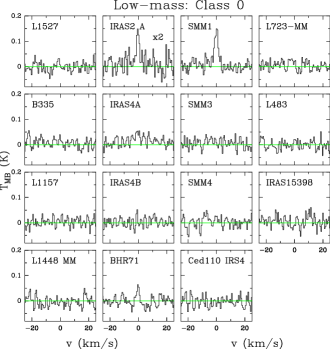
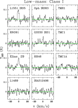
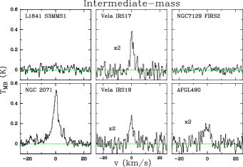
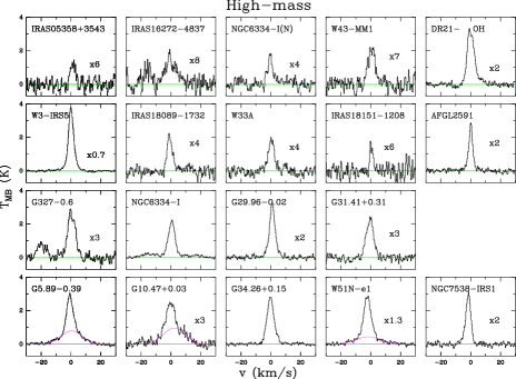
| Source | rmsa | c | |||
| (K km s-1) | (K) | (km s-1) | (mK) | (cm-2) | |
| Low-mass: Class 0 | |||||
| NGC 1333 IRAS 2A | 0.21 | 0.07 | 2.0 | 20 | 1.21021 |
| Ser SMM 1 | 0.70 | 0.13 | 3.0 | 23 | 4.11021 |
| Low-mass: Class I | |||||
| L 1551 IRS 5 | 0.22 | 0.10 | 3.1 | 24 | 1.31021 |
| GSS 30 IRS1 | 0.23 | 0.06 | 2.2 | 25 | 1.41021 |
| Elias 29 | 0.40 | 0.08 | 3.9 | 30 | 2.31021 |
| Intermediate-mass | |||||
| Vela IRS 19 | 0.37 | 0.11 | 3.2 | 24 | 2.21021 |
| Vela IRS 17 | 0.69 | 0.16 | 2.8 | 25 | 4.01021 |
| NGC 2071 | 2.97 | 0.41 | 4.6 | 25 | 1.71022 |
| AFGL 490 | 0.45 | 0.08 | 5.4 | 20 | 2.61021 |
| High-mass | |||||
| IRAS05358+3543 | 0.93 | 0.22 | 4.0 | 56 | 5.41021 |
| IRAS162724837 | 1.18 | 0.14 | 5.9 | 55 | 6.91021 |
| NGC6334-I(N) | 1.82 | 0.37 | 3.9 | 55 | 1.11022 |
| W43-MM1 | 1.81 | 0.29 | 5.9 | 49 | 1.01022 |
| DR21(OH) | 9.11 | 1.51 | 5.5 | 57 | 5.31022 |
| W3-IRS5 | 25.43 | 4.80 | 4.2 | 66 | 1.51023 |
| IRAS180891732 | 3.26 | 0.52 | 4.1 | 53 | 1.91022 |
| W33A | 3.17 | 0.43 | 4.8 | 46 | 1.91022 |
| IRAS181511208 | 0.60 | 0.24 | 4.2 | 54 | 3.51021 |
| AFGL2591 | 4.56 | 1.21 | 3.1 | 39 | 2.71022 |
| G3270.6 | 6.16 | 0.83 | 6.1 | 57 | 3.61022 |
| NGC6334-I | 10.97 | 2.00 | 5.0 | 54 | 6.41022 |
| G29.960.02 | 7.50 | 1.41 | 4.3 | 41 | 4.41022 |
| G31.41+0.31 | 5.26 | 0.73 | 6.0 | 36 | 3.11022 |
| G5.890.39d | 31.35 | 2.13 | 5.9 | 51 | 1.81023 |
| G10.47+0.03d | 5.71 | 0.53 | 6.4 | 79 | 1.11023 |
| G34.26+0.15 | 16.26 | 2.53 | 5.5 | 49 | 9.51022 |
| W51N-e1d | 15.22 | 1.83 | 5.7 | 48 | 8.91022 |
| NGC7538-IRS1 | 6.32 | 1.37 | 4.0 | 48 | 3.71022 |
Notes. (a) In 0.27 km s-1 bins.
(b) Integrated over the entire line.
(c) Column density of H2 calculated for an excitation temperature of 75 K and a C18O/H2
abundance ratio of 510-7.
(d) Two Gaussian fit. Only the values from the narrow velocity component are presented.
Finally, the C18O =10–9 transition was observed in 30 minute exposures for all low-mass Class 0 protostars, one intermediate-mass source and all high-mass YSOs. Additional deeper integrations of 300 minutes were obtained for NGC1333 IRAS 2A (as part of WISH) and for NGC1333 IRAS 4A, NGC1333 IRAS 4B, Elias 29 and GSS 30 IRS1 (as part of open-time programme OT2_rvisser_2) in parallel with deep HO searches. The line was detected in five low-mass sources and in all 19 high-mass objects (Fig. 19). This line appears close to the 1097 GHz H2O 3 transition. For most of the high-mass objects, the line profile of this water transition shows broad wings which extend few km s-1, so the C18O =10–9 emission line is found on top of the broad water red wing. In order to properly analyse the emission of this CO isotopologue, the line wings of the 1097 GHz water transition were fitted with a Gaussian profile, subtracted and the residuals plotted. With this method, the C18O =10–9 emission line for the high-mass sample has been isolated. The temperature of the gas that =10–9 traces is likely similar to that traced by the =9–8 transition, so the lines are also weak with median values of of 0.04 K for the low-mass protostars and 0.52 K for the high-mass objects. The FWHM of the one single Gaussian profile which fits these lines are slightly larger, ranging from 3.4 to 7.5 km s-1 for the high-mass sources (Table 9 for more details).
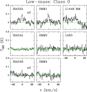
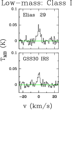
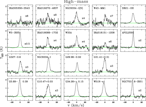
| Source | rmsa | |||
| (K km s-1) | (K) | (km s-1) | (mK) | |
| Low-mass: Class 0 | ||||
| NGC 1333 IRAS 2A | 0.34 | 0.04 | 10.7 | 8 |
| NGC 1333 IRAS 4B | 0.05 | 0.03 | 1.4 | 10 |
| Ser SMM 1 | 0.61 | 0.07 | 4.8 | 17 |
| Low-mass: Class I | ||||
| GSS 30 IRS1 | 0.12 | 0.04 | 3.1 | 8 |
| Elias 29 | 0.22 | 0.04 | 4.7 | 7 |
| High-mass | ||||
| IRAS05358+3543 | 0.42 | 0.10 | 3.8 | 26 |
| IRAS162724837 | 0.49 | 0.11 | 4.8 | 26 |
| NGC6334-I(N) | 2.31 | 0.28 | 7.5 | 20 |
| W43-MM1 | 0.92 | 0.12 | 5.3 | 23 |
| DR21(OH) | 7.94 | 1.08 | 6.0 | 33 |
| W3-IRS5 | 17.04 | 3.39 | 4.1 | 22 |
| IRAS180891732 | 1.54 | 0.30 | 4.5 | 28 |
| W33A | 1.72 | 0.30 | 4.3 | 22 |
| IRAS181511208 | 0.48 | 0.09 | 4.2 | 22 |
| AFGL2591 | 3.80 | 0.88 | 3.4 | 23 |
| G3270.6 | 3.03 | 0.42 | 5.8 | 34 |
| NGC6334-I | 10.09 | 1.55 | 5.3 | 28 |
| G29.960.02 | 5.79 | 1.02 | 4.5 | 30 |
| G31.41+0.31 | 3.98 | 0.52 | 6.1 | 38 |
| G5.890.39 | 11.59 | 2.08 | 7.0 | 27 |
| G10.47+0.03 | 3.44 | 0.47 | 7.1 | 26 |
| G34.26+0.15 | 11.80 | 1.73 | 6.0 | 29 |
| W51N-e1 | 10.49 | 1.48 | 6.8 | 52 |
| NGC7538-IRS1 | 3.95 | 0.88 | 3.9 | 37 |
Notes. (a) In 0.27 km s-1 bins.
(b) Integrated over the entire line.
Appendix B JCMT data
The central spectrum of the 12CO and C18O =3–2 spectral maps observed with the HARP instrument of the JCMT are presented in this section (see Figs. 23 and 24). These central spectra were convolved to a 20 beam in order to compare them with the HIFI data. The 12CO and C18O =3–2 spectra for the low-mass sources BHR 71, Ced110 IRS4, IRAS 12496 and HH 46 were observed with APEX because of their low declination. Similarly to the JCMT data, the central spectrum was convolved to a 20 beam. See Yıldız et al. (2013, submitted) for more information about the low-mass protostar observations.
The spectral maps are not presented in this paper because only the values of FWHM from the broad component for the 12CO =3–2 central spectrum were used in the analysis and discussion, together with the width and integrated intensity of the C18O =3–2 data. These values are presented in Table 10. Some spectra from these species are also plotted together with the HIFI data in the figures shown in this appendix in order to make a direct comparison of the lines for different types of protostars.
The 12CO =3–2 data show more complex line profiles than the =10–9, as indicated in Section 3.1, with intense self-absorption features and broad velocity components (see spectra from Fig. 23). More than 82% of the observed and detected lines (39 out of 47) present a broad velocity component, and the FWHM ranges from 7.4 to 53.3 km s-1, values corresponding to a low- and high-mass YSOs respectively.
On the other hand, the narrow C18O =3–2 spectra show single Gaussian emission profiles, similar to those from higher- transitions observed with HIFI. The FWHM of these data varies from 0.6 to 7.3 km s-1. The spectra is presented in Fig. 24 and the constrained values of FWHM and integrated intensity in Table 10.
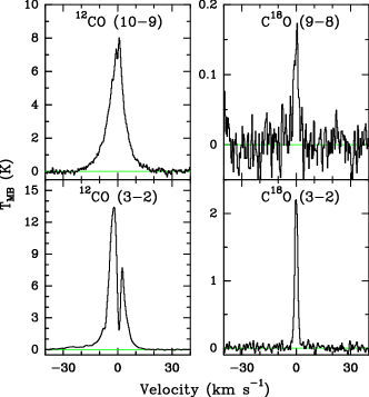
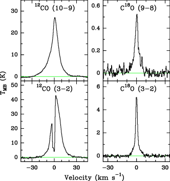
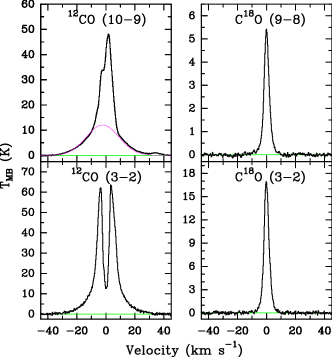
| Source | 12CO =3-2 | C18O =3-2 | |
|---|---|---|---|
| FWHMB | FWHM | ||
| (km s-1) | (km s-1) | (K km s-1) | |
| Low-mass: Class 0 | |||
| L 1448-MM | 18.5 | 1.1 | 1.5 |
| NGC 1333 IRAS2A | 13.8 | 1.2 | 2.8 |
| NGC 1333 IRAS4A | 20.1 | 1.5 | 2.5 |
| NGC 1333 IRAS4B | 16.2 | 0.8 | 1.6 |
| L 1527a | 0.7 | 1.5 | |
| Ced110 IRS4a | |||
| BHR 71 | 16.4 | 1.2 | 4.1 |
| IRAS 15398a | 0.7 | 0.8 | |
| L 483-MM | 10.2 | 0.6 | 1.2 |
| Ser SMM1 | 14.1 | 2.1 | 4.8 |
| Ser SMM4 | 14.2 | 2.3 | 6.0 |
| Ser SMM3 | 11.6 | 1.7 | 4.9 |
| L 723-MM | 13.2 | 1.5 | 1.0 |
| B 335a | 0.8 | 1.4 | |
| L 1157 | 18.9 | 0.9 | 0.6 |
| Low-mass: Class I | |||
| L 1489a | 2.0 | 0.7 | |
| L 1551-IRS5 | 10.4 | 0.9 | 2.3 |
| TMR1a | 1.2 | 1.1 | |
| TMC1 | 13.7 | 0.7 | 0.9 |
| TMC1A | 10.2 | 1.0 | 0.9 |
| HH46 | 12.8 | 0.9 | 3.2 |
| IRAS 12496 | 19.5 | 1.2 | 1.4 |
| Elias 29 | 7.8 | 2.5 | 5.3 |
| Oph IRS 63 | 8.5 | 0.6 | 1.1 |
| GSS 30-IRS1 | 7.4 | 1.2 | 3.7 |
| RNO 91 | 9.3 | 0.6 | 1.1 |
| Intermediate-mass | |||
| NGC 7129 FIRS2 | 18.2 | 1.6 | 5.1 |
| L1641 S3 MMS1 | 13.3 | 1.6 | 6.4 |
| NGC2071 | 25.5 | 2.8 | 14.1 |
| AFGL 490 | 37.4 | 2.3 | 13.2 |
| High-mass | |||
| IRAS05358+3543 | 20.0 | 3.0 | 7.7 |
| NGC6334-I(N) | 30.1 | ||
| W43-MM1 | 27.6 | 6.7 | 36.9 |
| DR21-OH | 5.5 | 49.8 | |
| W3-IRS5 | 24.7 | 4.2 | 76.1 |
| IRAS18089-1732 | 15.7 | 4.1 | 39.7 |
| W33A | 36.7 | 4.3 | 41.7 |
| IRAS18151-1208 a | 2.5 | 19.3 | |
| AFGL2591 | 22.0 | 3.6 | 45.9 |
| NGC6334-I | 35.7 | 3.7 | 50.3 |
| G29.96-0.02 | 18.0 | 4.0 | 65.9 |
| G31.41+0.31 | 24.9 | 7.3 | 44.5 |
| G5.89-0.39 | 53.5 | 4.8 | 95.0 |
| G10.47+0.03 | 14.1 | 7.0 | 82.2 |
| G34.26+0.15 | 23.9 | 6.0 | 153.2 |
| W51-e1 | 30.3 | ||
| NGC7538-IRS1 | 20.8 | 5.9 | 50.3 |
Notes. (a) No broad velocity component identified in the 12CO =3-2 convolved central spectrum.