One-loop photon-photon scattering in a thermal, deconfining SU(2) Yang-Mills plasma
Niko Krasowski and Ralf Hofmann^∗

Institut für Theoretische Physik

Universität Heidelberg

Philosophenweg 16

69120 Heidelberg, Germany

For a deconfining thermal SU(2) Yang-Mills plasma we discuss the role of (anti)calorons in introducing non-thermal behavior effectively described in terms of Planck’s quantum of action $\hbar$. This non-thermality cancels exactly between the ground-state estimate and its free quasiparticle excitations. Kinematic constraints in 4-vertex scattering and the counting of radial loop variables versus the number of independent constraints on them are re-visited. Next, we consider thermal 2$\rightarrow$ 2 one-loop scattering of the modes remaining massless upon the (anti)caloron induced adjoint Higgs mechanism (thermal ground state after spatial coarse graining). Starting with stringent analytical arguments, we are able to exclude the contribution to photon-photon scattering from diagrams containing at least one three-vertex and, in a next step, a vast majority of all possible configurations involving two four-vertices. By numerical analysis we show that the remaining contribution of the overall S channel is severely suppressed compared to that of the T and U channels, meaning that the creation of a pair of massive vector modes by a pair of photons and vice versa practically does not occur in the Yang-Mills plasma. For the T and U channels the domain of loop integration represents less than $10^{-7}$ times the volume of the unconstrained integration region. The thus introduced photon-photon correlation should affect the Cosmic Microwave Background’s polarisation at low redshift. An adaption of the here-developed methods to the analysis of irreducible bubble diagrams could prove the conjecture of hep-th/0609033 on the termination of the loop expansion of thermodynamical quantities at a finite irreducible order.

^∗email: r.hofmann@thphys.uni-heidelberg.de

1 Introduction

Effective, indeterministic behavior, inherent to scattering amplitudes in quantum Yang-Mills theory, appears to be associated with the presence of classical field configurations of finite action and nontrivial topology in 4D Euclidean spacetime [1, 2, 3, 4]. For SU(2) Yang-Mills thermodynamics a concrete argument in favor of this idea was put forward recently [5, 6]. Namely, in its deconfining phase an adjoint Higgs mechanism, caused by calorons and anicalorons of topological charge modulus unity, which, upon spatial coarse graining [7], effectively materialize in terms of an inert scalar field $\phi$, splits the Yang-Mills mass spectrum into two degenerate modes propagating on their quasiparticle mass-shell (unitary gauge) and a massless mode (photon) whose off-shellness is constrained by $|\phi|$ (Coulomb gauge) [8]. Moreover, (anti)caloron mediated 4-vertices (and 3-vertices) are pointlike in the effective theory because four-momentum transfer through them is restricted by $|\phi|$ in all Mandelstam variables. The present paper intents to investigates the consequences of these constraints for photon-photon scattering in the effective theory for the deconfining phase. However, before performing the according analysis, we would like to elaborate on the argument for and the implied consequences of (anti)caloron mediation of scattering in effective Yang-Mills vertices. To do so, we work in units where $c$, the speed of light in vacuum, is set to unity but Boltzmann’s constant $k_{B}$ and Planck’s quantum of action $\hbar$ are dimensionful.

Due to Feynman [9, 10] and Schwinger [11] the fundamental Yang-Mills partition function $Z$ is representable in fundamental variables as follows

$$Z\equiv\mbox{tr }e^{-\frac{\beta}{k_{B}}\mathcal{H}}=\sum_{n}\langle\left.n\right|\mbox{tr }e^{-\frac{\beta}{k_{B}}\mathcal{H}}\left|n\right.\rangle=\int_{A_{\mu}\left(0,\mathbf{x}\right)=A_{\mu}\left(\beta,\mathbf{x}\right)}\mathcal{D}A\,\mbox{e}^{-\frac{1}{k_{B}}\int_{0}^{\beta}d\tau^{\prime}\,d^{3}x\,\mathcal{L}_{E}\left[A_{\mu}\right]}\,.$$ (1)

where $\beta\equiv T^{-1}$, $T$ denotes temperature, $\mathcal{H}$ represents the Hamiltonian of quantum Yang-Mills theory, the functional integration is over gauge-inequivalent, periodic field configurations, and $\mathcal{L}_{E}$ refers to the classical Euclidean action density. In evaluating partition function (1), a simplification occurs if the quantum states $|n\rangle$ are taken to be (gauge-inequivalent) energy eigenstates of ${\cal H}$ with eigenvalues $E_{m}$. Formally, the partition function then reads

$$Z=\sum_{m}M(m)e^{-\frac{\beta E_{m}}{k_{B}}}\,.$$ (2)

Here $M(m)$ denotes the degeneracy of $E_{m}$. Resorting to a represention of the Hilbert space in field variables, ${\cal H}$ is a gauge-invariant functional of gauge field $A_{\mu}$ and its conjugate momentum $\Pi_{\mu}$ whose quantization conditions (equal-time commutators of $A_{\mu}$ and $\Pi_{\mu}$) involve $\hbar$. In a Euclidean spacetime, the operator $\mbox{e}^{-\frac{\beta}{k_{B}}{\cal H}}$ formally evolves a state $|n\rangle$ in $\tau^{\prime}$ – a variable of dimension inverse temperature $T^{-1}$ – from $\tau^{\prime}=0$ to $\tau^{\prime}=\beta\equiv 1/T$ if $\tau^{\prime}$ and time $\tau$ are related as

$$\tau^{\prime}=\frac{k_{B}}{\hbar}\tau\ \ \ \ \mbox{or}\ \ \ \ \tau=\frac{\hbar}{k_{B}}\tau^{\prime}\,.$$ (3)

Now, neither the macroscopic concept time ($\tau$) nor the macroscopic concept temperature ($\tau^{\prime}$) ought to depend on the values of $\hbar$ and $k_{B}$. As a consequence, Eq. (3) implies that in the formal limit $\hbar\to 0$ also $k_{B}\to 0$ such that

$$\frac{\hbar}{k_{B}}=\mbox{const}\,.$$ (4)

Quantity $\langle n|\mbox{e}^{-\frac{\beta}{k_{B}}{\cal H}}|n\rangle$ thus represents the formal persistence amplitude for state $|n\rangle$ under (Euclidean) time evolution from $\tau=0$ to $\tau=\frac{\hbar}{k_{B}T}$.

If the world were purely thermal and Euclidean (no reference to a Wick rotated version of temporal evolution acting on a quantum state in Minkowski spacetime) on subatomic length scales then the concept of action would be inappropriate, and energy per temperature in units of $k_{B}$ would occur naturally in exponential weights representing the Yang-Mills spectrum. Conversely, if the subatomic world were purely Minkowskian and non-thermal then one would consider a summation over field ‘trajectories’ whose action in units of $\hbar$ weights their contributions to the temporal evolution of a given quantum state. Interestingly, thermal Quantum Yang-Mills theory emerges as an interplay of these two concepts. For example, the notion of the thermal ground state invokes the fact that the former point of view is related to the latter by representing effective variables nonlocally in terms of fundamental ones: The periodicity of these fundamental (classical, Euclidean) configurations (calorons and anticalorons) is a consequence of identification (3) which rests on temporal evolution of quantum states. Collectively, however, nontrivial, temporal periodicity collapses to a mere choice of gauge on the effective-theory level [8]. Alternatively, the occurrence of effective quantum corrections, expanded in powers of $\hbar$, is demanded by isolated action of (anti)calorons. In this context, hinging on adiabatic slowness to render Euclidean signature irrelevant, the physics of (anti)caloron constituents (monopole-antimonopole pair) can be interpreted classically [12, 13].

For the deconfining phase of SU(2) Yang-Mills thermodynamics we have in [5, 6] identified the Euclidean action of relevant calorons or anticalorons [14, 15, 16, 17] with $\hbar$. The according chain of arguments relies on a Minkowskian interpretation of free but effectively massive (adjoint Higgs mechanism) one-loop fluctuations about the ground-state estimate. Here the contribution of quasiparticles to the pressure, expressed by a Matsubara sum in Euclidean spacetime, is cast into a continuous integration by employing Cauchy’s integral theorem. Because of Minkowskian on-shellness (inertness of the adjoint scalar field $\phi$ [18]) only the Bose weighted part in the propagator contributes to the loop integration. Thermodynamic consistency (linking of thermodynamical quantities by Legendre transformations motivated by the left part of Eq. (1)) and a dimensional counting in effective interaction monomials with appropriately normalized field variables [19] determines the effective coupling $e$ in units of $\hbar^{-1/2}$ [5, 6]. Finally, one appeals to the observation that (anti)caloron radii $\rho\sim|\phi|^{-1}$ dominate the spatial coarse-graining – generating the field $\phi$ [7, 18] – to justify the use of $e$ in the formula $S=\frac{8\pi^{2}}{e^{2}}$ for the Euclidean action of the fundamental field configurations caloron or anticaloron with topological charge modulus unity. As an immediate consequence, pointlike effective vertices, introducing perturbations into thermally weighted Minkowskian on-shell propagation in terms of free plane waves, occur because these vertices effectively interpolate the incoming and the scattered wave through spatially unresolved (anti)calorons subject to a Euclidean time dependence. Here, the irreconcilability of Euclidean and Minkowskian time evolution within a vertex, represents the cause of effective indeterminism in the outcome of the scattering event: Wick rotation of a caloron’s time dependence generates a field configuration which is far from the nearest classical solution to the Minkowskian Yang-Mills equations. Effectively parametrized by $\hbar$, the action of isolated (anti)calorons thus introduces disorder to equilibrated Minkowskian plane-wave propagation. In this sense (anti)calorons behave non-thermally, resolving the following paradox associated with the ground-state estimate: While the latter, describing the interacting (anti)calorons in terms of the field $\phi$ and an effective, pure-gauge configuration $a_{\mu}^{\tiny\mbox{gs}}$, obeys an equation of state $P^{\tiny\mbox{gs}}=-\rho^{\tiny\mbox{gs}}$ it does exhibit a finite heat capacity. In other words, the ground state’s entropy density $s^{\tiny\mbox{gs}}$, given as

$$s{\tiny\mbox{gs}}\equiv\frac{1}{T}(P{\tiny\mbox{gs}}+\rho{\tiny\mbox{gs}})\,,$$ (5)

vanishes although $\rho^{\tiny\mbox{gs}}=4\pi T\Lambda^{3}$ is temperature dependent, $\Lambda$ denoting the Yang-Mills scale [8]. At finite temperature this violates the third law of thermodynamics. Therefore, a thermodynamical interpretation of the ground-state physics alone is not admissible. That this estimate does not behave thermodynamically by itself is, however, not a surprise because of the de-thermalizing effect of (anti)calorons constituting the thermal ground state. Modulo small radiative corrections, see below, the overall Yang-Mills system is thermodynamical, however: between the ground state and its quasiparticle excitations the $T$ dependence of the effective coupling $e$ cancels non-thermality [20]. When, at the critical temperature $T_{c^{\prime}}$ (lowest attainable temperature in the preconfining phase [8]), quasiparticles disappear entirely the thermal ground state would represent the entire thermal partition function which, by the above entropy argument, does not make sense. Indeed, the onset of the Hagedorn transition at $T_{c^{\prime}}$ explicitly violates a thermodynamical description of the Yang-Mills system [20]. Note that except for the limit $T\searrow T_{c}$ [8], where radiative corrections vanish [8], non-thermal effects are ubiquitous also in the deconfining and preconfining phases: there are small radiative corrections in the former phase, associated with fixed or resummed loop orders [21, 22, 23] which are triggered by isolated (anti)calorons, while supercooling and a related ground-state tunneling take place in the latter phase [20].

To conclude this discussion, we may simply state that the (deeply physical) demand for periodicity of any field configuration contributing to the reformulation of the partition function in terms of the functional integral in Eq. (1) is an extrapolation of the free-field case which introduces in principle non-thermal behavior: While the Minkowskian on-shell propagation of free plane waves becomes Bose-Einstein weighted as a consequence of this prescription it also allows for the contribution of topologically charged field configurations (calorons and anticalorons) which ultimately (low-temperature situation) destroy spatial translation invariance and which introduce an over-exponentially rising density of states in the confining phase. As long as the collective effect of (anti)calorons gives rise to spatially homogeneous effects only (e.g., energy density of the ground state or quasiparticle masses) thermodynamics is kept intact by cancellations of non-thermal effects between ground state and massive excitations, enabled by a proper tuning of the coupling (deconfining phases). Radiative corrections, however, are mediated by isolated (anti)caloron action, altering the propagation behavior of every single plane wave in a non-thermal way. We believe that this is the cause for the large-angle anomalies in the temperature fluctuations of the Cosmic Microwave Background presently discussed.

The present paper is organized as follows. In Sec. 2 we review the effective theory together with its constraints in unitary-Coulomb gauge, and we re-revisit the counting of constraints in dependence on loop order in irreducible diagrams subject to 4-vertices only. Sec. 3 discusses how these constraints apply to exclude certain one-loop diagrams potentially contributing to the photon-photon scattering amplitude. Moreover, a technology is developed that allows to systematically discriminate a number of channel combinations for the two 4-vertices in the remaining diagrams in this amplitude. For the remaining possibilities, where no further analytical assessment can be made, a Monte-Carlo simulation of the domain of integration is performed, and a selected hit is investigated further in view of its embedding into the extremely fillamented algebraic variety comprising a part of the domain of integration. The last section summarizes our results and gives conclusions.

2 Effective theory, notational conventions, and constraints

For the benefit of the reader we re-visit briefly the effective theory for deconfining SU(2) Yang-Mills thermodynamics and discuss its constraints on 4-vertices, see also [6, 18]. We also discuss an (inessential) correction to the counting of constraints for irreducible diagrams that arise solely from 4-vertices. From now on we work in supernatural units $\hbar=k_{B}=c=1$.

2.1 Effective action

The effective action for the deconfining phase emerges upon a spatial coarse-graining over free, trivial-holonomy (anti)calorons of charge modulus unity and plane-wave fluctuations [7]. While the topologically nontrivial sector of gauge-field configurations yields an inert, adjoint scalar field $\phi$ coarse-graining over interactions within the topologically trivial sector is determined by perturbative renormalizability to contribute to the effective action for the coarse-grained, topologically trivial gauge field $a_{\mu}$ in the same form as the fundamental Yang-Mills action [24, 25]. Moreover, the appearance of mixed operators of mass dimension higher than four, involving both fields $a_{\mu}$ and $\phi$, is excluded because momentum transfer to the field $\phi$ is impossible [18]. Thus the unique (Euclidean) density of effective action ${\cal L}_{\mbox{\tiny eff}}[a_{\mu}]$ is given as

$${\cal L}_{\mbox{\tiny eff}}[a_{\mu}]=\mbox{tr}\,\left(\frac{1}{2}\,G_{\mu\nu}G_{\mu\nu}+(D_{\mu}\phi)^{2}+\frac{\Lambda^{6}}{\phi^{2}}\right)\,,$$ (6)

where $G_{\mu\nu}=\partial_{\mu}a_{\nu}-\partial_{\nu}a_{\mu}-ie[a_{\mu},a_{\nu}]\equiv G_{\mu\nu}^{a}\,t_{a}$ denotes the field strength, $D_{\mu}\phi=\partial_{\mu}\phi-ie[a_{\mu},\phi]$, and $e$ is the effective gauge coupling yet to be determined. ${\cal L}_{\mbox{\tiny eff}}$ in Eq. (6) yields a highly accurate tree-level ground-state estimate and, as easily deduced in unitary gauge $\phi=2|\phi|\,t_{3}$, a tree-level mass $m=2\,e|\phi|=2\,e\sqrt{\frac{\Lambda^{3}}{2\pi T}}$ for propagating gauge modes $a_{\mu}^{1,2}$. Because the mass of these modes is generated by a summation of a Dyson series of up to infinitely many local interactions with the field $\phi^{2}$ the off-shellness inducing absorption or emission of effective, propagating modes is forbidden: these processes would introduce momentum transfer to the inert field $\phi$. As a consequence, massive modes propagate thermally on their mass shell [18]. Massless modes (photons), on the other hand, may be off their mass shell at most by $|\phi|^{2}$ [8]. Finally, thermodynamical consistency of the system’s ground-state estimate and its free quasiparticles yields the value $e=\sqrt{8}\pi$ almost everywhere. The exception is a narrow, logarithmic pole at $T_{c}=13.87\,\frac{\Lambda}{2\pi}$.

Considering radiative corrections, the effective 3- and 4-vertices are given as

$$\Gamma_{[3]\,abc}^{\alpha\beta\gamma}= \,e(2\pi)^{4}\delta(p_{A}+p_{B}+p_{C})\epsilon_{abc}\times\left[g^{\alpha\beta}\left(p_{B}-p_{A}\right)^{\gamma}\right.$$

$$\left.+g^{\beta\gamma}\left(p_{C}-p_{B}\right)^{\alpha}+g^{\gamma\alpha}\left(p_{A}-p_{C}\right)^{\beta}\right]\,,$$ (7)

$$\Gamma_{[4]\,abcd}^{\alpha\beta\gamma\delta}= -\mathrm{i}e^{2}(2\pi)^{4}\delta(p_{A}+p_{B}+p_{C}+p_{D})\times\left[\epsilon_{abe}\epsilon_{cde}(g^{\alpha\gamma}g^{\beta\delta}-g^{\alpha\delta}g^{\beta\gamma})\right.$$

$$\left.+\epsilon_{ace}\epsilon_{bde}(g^{\alpha\beta}g^{\gamma\delta}-g^{\alpha\delta}g^{\beta\gamma})+\epsilon_{ade}\epsilon_{bce}(g^{\alpha\beta}g^{\gamma\delta}-g^{\alpha\gamma}g^{\beta\delta})\right]\,,$$ (8)

compare with Fig. 1.

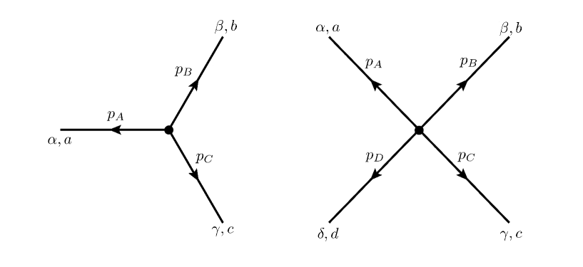
Figure 1: Yang-Mills vertices, $p_{X}$ being a four-momentum, greek letters are Lorentz indices, lower case latin letters denote Lie-Algebra indices.

In the present paper, no explicit reference to propagators is made except for the above mentioned fact that massive modes always are on-shell. Let us now set up our notational conventions.
Vertices. Vertices are discussed on different levels. Some arguments require only formulas that are valid independently of the sort of attached gauge modes. In such cases we just use the symbols $p_{1}$, $p_{2}$ etc. for four-momenta. On a level, where we would like to distinguish between massive and massless modes, we use $R$, $S$, $P$ for the four-momenta of the massive modes and $p$, $q$ for the four-momenta of photons. In applications to the actual scattering process we employ $a$ and $b$ to indicate the four-momenta of incoming photons. Outgoing photons are labeled by $c$ and $d$. Four-momenta of internal, massive (loop) modes are denoted by $u$ and $v$.
Feynman diagrams. In general, the propagation of massive particles is indicated by double lines in Feynman diagrams while massless modes are represented by single lines (except for Fig. 2 where a wavy line is used).
Scattering channels. An overall channel in photon-photon scattering is labeled by the Mandelstam variable S,T or U (captial letters). On the other hand, for scattering channels associated with a given 4-vertex Mandelstam variables are in lower case letters. In this way, one specific configuration can be written in a short-hand notation. For example, “Stu” describes overall S-channel scattering with the t-channel realized at the first 4-vertex and the u-channel at the second 4-vertex.

2.2 3-vertex

At the 3-vertex, given as in Eq. (7), a photon always connects to two massive modes .

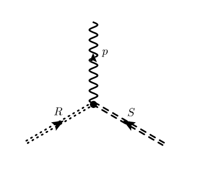
Figure 2: Two different massive modes (dashed and dotted) and a massless one (wavy) at a 3-vertex.

For later use let us now check whether the photon can be an external, on-shell particle of positive energy . Because of four-momentum conservation and the on-shellness of the massive modes the following conditions apply:

$$R^{2}=S^{2} =m^{2}\,,$$

$$p^{2} =0\,,$$

$$(R+S)^{2} =p^{2}=0\,.$$ (9)

The energy of the massive particles can be positive or negative, depending on the direction of energy flow in the loop of the overal scattering diagram, see Fig. 3.

Figure 3: Box diagram (left) and penguin diagram (right). Both possibilities are excluded to contribute to photon-photon scattering.

Therefore, one has

$$2m^{2}\pm 2\sqrt{\left|\mathbf{R}\right|+m^{2}}\sqrt{\left|\mathbf{S}\right|^{2}+m^{2}}-2\mathbf{R}\mathbf{S} =0$$

$${\mbox{upon squaring}}\,\Rightarrow\;\;\left(\left|\mathbf{R}\right|^{2}+m^{2}\right)\left(\left|\mathbf{S}\right|^{2}+m^{2}\right)-m^{4}-\left(\mathbf{R}\mathbf{S}\right)^{2}+2m^{2}\mathbf{R}\mathbf{S} =0$$

$$\Rightarrow\;\;m^{2}\left(\left|\mathbf{R}\right|^{2}+\left|\mathbf{S}\right|^{2}+2\left|\mathbf{R}\right|\left|\mathbf{S}\right|\cos\measuredangle(\mathbf{R},\mathbf{S})\right)$$

$$+|\mathbf{R}|^{{}^{2}}\left|\mathbf{S}\right|^{2}\left(1-\cos^{2}\measuredangle(\mathbf{R},\mathbf{S})\right) =0\,.$$ (10)

The minimal value of each summand in the last equation of (10) is zero: The first summand vanishes for $\cos\measuredangle(\mathbf{R},\mathbf{S})=-1$ and $\left|\mathbf{R}\right|=\left|\mathbf{S}\right|$, the second summand is zero for $\cos\measuredangle(\mathbf{R},\mathbf{S})=\pm 1$. So the only configuration satisfying Eq. (10) is $\measuredangle(\mathbf{R},\mathbf{S})=\pi$ and equal energy of the photons. Since in a loop integral the thus allowed integration over angular variables is over a hypersurface of measure zero we conclude that 3-vertices do not contribute to the overall one-loop scattering of photons.

2.3 Constraints on 4-vertex

It is easy to show that the 4-vertex is invariant under a permutation of the legs attached to it [26]. This implies that the 4-vertex does not distinguish between Mandelstam variables $s,t,$ and $u$ in mediating 2$\to$2 scattering. The according constraints, however, do. It is also straightforward to demonstrate that, modulo leg permutation, only the two diagrams depicted in Fig. 4 take place.

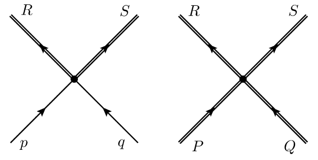
Figure 4: Photon-photon to massive-massive and massive-massive to massive-massive scattering. These are the cases that need to be distinguished in all scattering channels.

In the effective theory one has [8]

$$s=\left|\left(p_{1}+p_{2}\right)^{2}\right|=\left|\left(p_{3}+p_{4}\right)^{2}\right|\leq\left|\phi\right|^{2}\,,$$ (11)

$$t=\left|\left(p_{1}-p_{3}\right)^{2}\right|=\left|\left(p_{2}-p_{4}\right)^{2}\right|\leq\left|\phi\right|^{2}\,,$$ (12)

$$u=\left|\left(p_{2}-p_{3}\right)^{2}\right|=\left|\left(p_{1}-p_{4}\right)^{2}\right|\leq\left|\phi\right|^{2}\,$$ (13)

for a scattering amplitude mediated by a 4-vertex with momentum labeling as defined in Fig. 5.

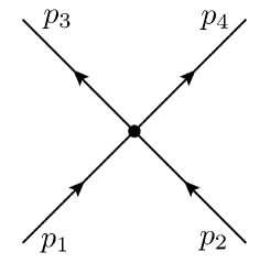
Figure 5: Scattering due to a 4-vertex.

Specializing to the situation of Fig. 4 and introducing $x\in\{p,P\}$ to cover both diagrams, we have

$$s= \left|\left(R+S\right)^{2}\right|\leq\left|\phi\right|^{2}\,,$$ (14)

$$t= \left|\left(x-R\right)^{2}\right|\leq\left|\phi\right|^{2}\,,$$ (15)

$$u= \left|\left(x-S\right)^{2}\right|\leq\left|\phi\right|^{2}\,.$$ (16)

Let us now show that it is impossible to satisfy each of these constraints simultaneously. Appealing to Eqs. (14) through (16) and using $P^{2}=Q^{2}=R^{2}=S^{2}=m^{2}$, $p^{2}=0$, one arrives at the following constraints for the case of two photons, two massive modes (left) and four massive modes (right):

two photons, two massive modes: $$s=|2R_{0}S_{0}+2m^{2}-2\mathbf{R}\mathbf{S}|\leq|\phi|^{2}\,,$$ (17) $$t=|-2p_{0}R_{0}+m^{2}+2\mathbf{p}\mathbf{R}|\leq|\phi|^{2}\,,$$ (18) $$u=|-2p_{0}S_{0}+m^{2}+2\mathbf{p}\mathbf{S}|\leq|\phi|^{2}\,,$$ (19)

four massive modes: $$s=|2R_{0}S_{0}+2m^{2}-2\mathbf{R}\mathbf{S}|\leq|\phi|^{2}\,,\,\,\,\,$$ (20) $$t=|-2R_{0}P_{0}+2m^{2}+2\mathbf{R}\mathbf{P}|\leq|\phi|^{2}\,,$$ (21) $$u=|-2S_{0}P_{0}+2m^{2}+2\mathbf{S}\mathbf{P}|\leq|\phi|^{2}\,.$$ (22)

We have

$$|2p_{0}R_{0}|>|2p_{0}(\sqrt{R_{0}^{2}-m^{2}})\cos\left(\measuredangle\left(\mathbf{p},\mathbf{R}\right)\right)|=|2\mathbf{p}\mathbf{R}|\,,$$ (23)

$$|2R_{0}S_{0}|>|2(\sqrt{R_{0}^{2}-m^{2}}\sqrt{S_{0}^{2}-m^{2}})\cos(\measuredangle\left(\mbox{$\mathbf{R}$,$\mathbf{S}$}\right))|=|2\mathbf{R}\mathbf{S}|\,.$$ (24)

The following argument does not rely on a restriction of the signs of the energies $p_{0}$, $R_{0}$, and $S_{0}$. From (24) and the fact that $m^{2}>|\phi|^{2}$ it follows that the sign of both $R_{0}$ and $S_{0}$ in (17) need to be different. Similar conclusions can be drawn for the other five cases (18) through (22). Again, using variable $x\in\{p,P\}$, we can summarize the situation as

$$s\leq|\phi|^{2}\Rightarrow\mbox{sgn}(R_{0}) \,=-\mbox{sgn}(S_{0})\,,$$

$$t\leq|\phi|^{2}\Rightarrow\,\mbox{sgn}(x_{0}) \,=\mbox{sgn}(R_{0})\,,$$

$$u\leq|\phi|^{2}\Rightarrow\,\mbox{sgn}(x_{0}) \,=\mbox{sgn}(S_{0})\,.$$

Therefore, one arrives at the following statement:

$$\mbox{sgn}(x_{0})=\mbox{sgn}(R_{0})=-\mbox{sgn}(S_{0})=-\mbox{sgn}(x_{0})\,.$$ (25)

As a consequence, the constraints (18) through (19) or (20) through (22) can not be satisfied simultaneously. Thus, rather than imposing all constraints simultaneously at a given 4-vertex, a weighted superposition of allowed 2$\to$ 2 diagrams, satisfying only one momentum-transfer constraint for $s$, $t$, or $u$ at a time, is to be considered. As mentioned above, the 4-vertex is blind to permutations of legs, i.e. it treats every scattering channel in the same way. For the case, where none of the constraints (18) through (22) is trivial, this leads to the following prescription for the implementation of a 4-vertex in the effective theory [6]:

$$\Gamma_{\left[4\right]abcd}^{\alpha\beta\gamma\delta}=\frac{1}{3}\left(\left.\Gamma_{\left[4\right]abcd}^{\alpha\beta\gamma\delta}\right|_{s}+\left.\Gamma_{\left[4\right]abcd}^{\alpha\beta\gamma\delta}\right|_{t}+\left.\Gamma_{\left[4\right]abcd}^{\alpha\beta\gamma\delta}\right|_{u}\right)\,.$$ (26)

If, on the other hand, say, the $t$ channel is trivial (polarization tensor of the massless mode on the one-loop level or figure-eight two-loop contributions to the pressure [21, 22]) then the vertex acts as [6]

$$\Gamma_{\left[4\right]abcd}^{\alpha\beta\gamma\delta}=\frac{1}{2}\left(\left.\Gamma_{\left[4\right]abcd}^{\alpha\beta\gamma\delta}\right|_{s}+\left.\Gamma_{\left[4\right]abcd}^{\alpha\beta\gamma\delta}\right|_{u}\right)\,.$$ (27)

This decomposition of a given 4-vertex into its scattering channels is the reason for the large number of $3^{3}=27$ possible scattering channel combinations in the three overall channels for one-loop photon-photon scattering, compare with Fig. 6

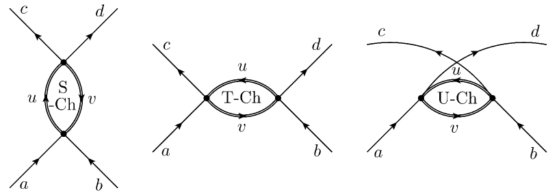
Figure 6: The overall scattering channels for the only admissible class of diagrams (two 4-vertices) in one-loop photon-photon scattering. Here $a$,$b$,$c$, and $d$ are the four-momenta of the photons, and $u$ and $v$ denote the loop four-momenta of the massive modes.

2.4 Energy-flow constraints

Let us now investigate all possible constraints that can occur in one-loop photon-photon scattering in view of energy flow. To do this, it is advantageous to work with dimensionless quantities. We will use two different normalizations. A tilde on top of a four-momentum component $x$ marks normalizations with respect to the modulus of the adjoint scalar field $\left|\phi\right|$, a hat denotes normalization with respect to the temperature $T$, e.g.

$$\tilde{x}\equiv\frac{x}{\left|\phi\right|}=\frac{2e}{m}x=\frac{\lambda^{\frac{3}{2}}}{2\pi}\frac{x}{T}\equiv\frac{\lambda^{\frac{3}{2}}}{2\pi}\hat{x}\,,$$ (28)

where the dimensionless temperature $\lambda$ is defined as

$$\lambda\equiv\frac{2\pi T}{\Lambda}\,.$$ (29)

Furthermore, the dimensionless mass $\tilde{m}\equiv\frac{m}{\left|\phi\right|}$ is given as

$$\tilde{m}= 2e\,,$$ (30)

where $e\geq\sqrt{8}\pi$ [20].

For a 4-vertex connecting two photons (four-momenta $\tilde{p}$, $\tilde{q}$) with two massive modes (four-momenta $\tilde{R}$, $\tilde{S}$) simple combinatorics allows the following possibilities of momentum transfer through the vertex, redundant by four-momentum conservation and constrained by the maximal resolution $|\phi|$ of the effective theory:

$$\left|\left(\tilde{R}\pm\tilde{S}\right)^{2}\right| \leq 1$$ (31)

$$\left|\left(\tilde{p}\pm\tilde{R}\right)^{2}\right| \leq 1$$ (32)

$$\left|\left(\tilde{p}\pm\tilde{S}\right)^{2}\right| \leq 1$$ (33)

$$\left|\left(\tilde{q}\pm\tilde{R}\right)^{2}\right| \leq 1$$ (34)

$$\left|\left(\tilde{q}\pm\tilde{S}\right)^{2}\right| \leq 1$$ (35)

$$\left|\left(\tilde{p}\pm\tilde{q}\right)^{2}\right| \leq 1\,.$$ (36)

Both, photons and massive modes are on shell:

$$\tilde{R}_{0} =\pm\sqrt{\left|\mathbf{\mathbf{\tilde{R}}}\right|^{2}+\tilde{m}^{2}}\,,$$ (37)

$$\tilde{S}_{0} =\pm\sqrt{\left|\mathbf{\mathbf{\tilde{S}}}\right|^{2}+\tilde{m}^{2}}\,,$$ (38)

$$\tilde{p}^{2} =0\,,$$ (39)

$$\tilde{q}^{2} =0\,.$$ (40)

¿From Eqs. (30) and (37) through (40) it follows that certain sign combinations of $R_{0}$ and $S_{0}$ are forbidden. Let us now classify those excluded cases. We consider

$$1\geq \left|\left(\tilde{R}\pm\tilde{S}\right)^{2}\right|=\left|2\tilde{m}^{2}\pm 2\tilde{R}_{0}\tilde{S}_{0}\mp 2\mathbf{\tilde{R}}\mathbf{\tilde{S}}\right|$$

$$= \left|2\tilde{m}^{2}\pm 2\left(\pm\sqrt{\left|\mathbf{\tilde{R}}\right|^{2}+\tilde{m}^{2}}\right)\left(\pm\sqrt{\left|\mathbf{\tilde{S}}\right|^{2}+\tilde{m}^{2}}\right)\mp 2\mathbf{\tilde{R}}\mathbf{\tilde{S}}\right|$$ (41)

and

$$1\geq \left|\left(\tilde{p}\pm\tilde{R}\right)^{2}\right|=\left|\tilde{m}^{2}\pm 2\tilde{p}_{0}\tilde{R}_{0}\mp 2\mathbf{\tilde{p}}\mathbf{\tilde{R}}\right|$$

$$= \left|\tilde{m}^{2}\pm 2\tilde{p}_{0}\left(\pm\sqrt{\left|\mathbf{\tilde{R}}\right|^{2}+\tilde{m}^{2}}\right)\mp 2\mathbf{\tilde{p}}\mathbf{\tilde{R}}\right|\,.$$ (42)

In the following discussion cases (31) are treated in terms of (41) while cases (32) through (35) are covered by (42). To proceed, note that

$$\left|\left(\pm\sqrt{\left|\mathbf{\tilde{R}}\right|^{2}+\tilde{m}^{2}}\right)\left(\pm\sqrt{\left|\mathbf{\tilde{S}}\right|^{2}+\tilde{m}^{2}}\right)\right|\mp\mathbf{\tilde{R}}\mathbf{\tilde{S}}\geq\tilde{m}^{2}$$ (43)

and

$$\left|p_{0}\left(\pm\sqrt{\left|\mathbf{\tilde{R}}\right|^{2}+\tilde{m}^{2}}\right)\right|\mp\mathbf{\tilde{p}}\mathbf{\tilde{R}}\geq 0$$ (44)

Inequality (43) is true because of the Cauchy-Schwarz inequality applied to the two vectors $\left(\left|\mathbf{\tilde{R}}\right|,\tilde{m}\right)$ and $\left(\left|\mathbf{\tilde{S}}\right|,\tilde{m}\right)$ with the canonical scalar product of $\mathbb{R}^{2}$ and the fact that $\left|\cos\measuredangle\mathbf{\tilde{R}}\mathbf{\tilde{S}}\right|\leq 1$. Inequality (44) is selfevident. ¿From (43), $m^{2}>1$ (see (30)), and (41) it follows that

$$\mbox{sgn}\left(\tilde{R}_{0}\right)=\pm\mbox{sgn}\left(\tilde{S}_{0}\right)$$

are forbidden for cases (31), respectively. Because of (44), $\tilde{m}^{2}>1$, and (42) it is clear that

$$\mbox{sgn}\left(\tilde{R}_{0}\right)=\pm 1$$

are forbidden for cases (32), respectively (and for cases (34), respectively). In addition, the respective cases (33) and (35) ($\tilde{R}$ replaced by $\tilde{S}$) are also excluded. Obviously, no implication for the signs of $\tilde{R}_{\text{0}}$ or $\tilde{S}_{\text{0}}$ arises from (36).

2.5 Counting of constraints

Because a 4-vertex is constrained by one of the constraints (11), (12), or (13) only the estimate of the ratio of the number $\tilde{K}$ of independent, radial loop variables versus the number $K$ of constraints on them obtained in Eq. (5.101) of [6] or in Eq. (16) of [29] modifies as

$$\frac{\tilde{K}}{K}\leq\frac{4}{5}\left(1+\frac{1}{V_{4}}\right)$$ (45)

for the case of a planar diagram containing only $V_{4}$ many 4-vertices. This generalises to

$$\frac{\tilde{K}}{K}\leq\frac{4}{5}\left(1+\frac{1}{V_{4}}(1-2g)\right)$$ (46)

if the diagram exhibits a nontrivial genus $g$. For $g=0$ one has $\frac{\tilde{K}}{K}\leq 1$ provided that $V_{4}\geq 4$.

3 Photon-photon scattering

Let us now assess the options for one-loop photon-photon scattering. To do this, we first apply the results of Sec. 2.4 to each of the overall scattering channels depicted in Fig. 6. This excludes a vast majority of a priori thinkable energy-flow combinations. In the overall S-channel scattering channel all combinations for the two 4-vertices can be excluded by analytical arguments. For the overall T-channel (U-channel as well) the analytical treatment leaves four combinations possible. These are investigated by numerical analysis based on Monte-Carlo simulations.

At a given vertex, we use the following notation to keep track of excluded combinations of the two loop energies $u_{0}$ and $v_{0}$. Every cell in a $2\times 2$ table accounts for one possible combinations of energy flow:

$\tilde{u}_{0}>0;\>\tilde{v}_{0}>0$	$\tilde{u}_{0}>0;\>\tilde{v}_{0}<0$
$\tilde{u}_{0}<0;\>\tilde{v}_{0}>0$	$\tilde{u}_{0}<0;\>\tilde{v}_{0}<0$

.

An “X” in a given cell signals that the corresponding combination is forbidden.

3.1 Energy flow: Overall S channel

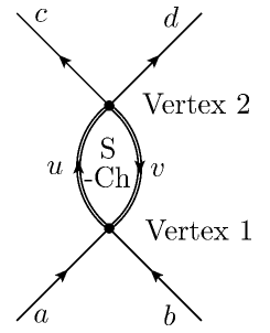
Figure 7: The overall S-channel.

The lower vertex in Fig. 7 is denoted by number 1, the upper one by number 2. At a given vertex the constraint on a scattering channel can be expressed in a twofold way because of total four-momentum conservation across the vertex. For example, the constraint at the first vertex $\left|\left(\tilde{a}+\tilde{b}\right)^{2}\right|\leq 1$ can be rewritten as $\left|\left(\tilde{u}-\tilde{v}\right)^{2}\right|\leq 1$. To exclude all sign combinations of the energies in the loop momenta one needs to look at either form and combine both statements .

Let us now visualize the constraints at vertex 1 in terms of their tables:

$\textnormal{s-ch:}\;\;1\geq\left|\left(\tilde{a}+\tilde{b}\right)^{2}\right|=\left|\left(\tilde{u}-\tilde{v}\right)^{2}\right|\rightarrow\>$ X X $\,,$

$\textnormal{t-ch:}\;\;1\geq\left|\left(\tilde{a}-\tilde{u}\right)^{2}\right|=\left|\left(\tilde{b}+\tilde{v}\right)^{2}\right|\rightarrow\>$ X X X $\,,$

$\textnormal{u-ch:}\;\;1\geq\left|\left(\tilde{a}+\tilde{v}\right)^{2}\right|=\left|\left(\tilde{b}-\tilde{u}\right)^{2}\right|\rightarrow\>$ X X X $\,.$

For vertex 2 we obtain:

$\textnormal{s-ch:}\;\;1\geq\left|\left(\tilde{u}-\tilde{v}\right)^{2}\right|=\left|\left(\tilde{c}+\tilde{d}\right)^{2}\right|\rightarrow\>$ X X $\,,$

$\textnormal{t-ch:}\;\;1\geq\left|\left(\tilde{u}-\tilde{c}\right)^{2}\right|=\left|\left(\tilde{v}+\tilde{d}\right)^{2}\right|\rightarrow\>$ X X X $\,,$

$\textnormal{u-ch:}\;\;1\geq\left|\left(\tilde{u}-\tilde{d}\right)^{2}\right|=\left|\left(\tilde{v}+\tilde{c}\right)^{2}\right|\rightarrow\>$ X X X $\,.$

In the diagram for the overall scattering channel (Fig. 7) the constraints on the two vertices have to be satisfied together in order to contribute: If one combination of energy flow and scattering channel is forbidden by one constraint then it is not allowed at all. Thus it is suggested to use a $3\times 3$ table for visualization of excluded scattering-channel and energy-flow combinations within a given overall channel. Each of the cells of this $3\times 3$ table, corresponding to a certain combination of scattering channels at vertex 1 and vertex 2, is obtained by putting the two respective $2\times 2$ tables on top of one another. For the overall S-channel we thus are left with Tab. 1.

		s-ch.			t-ch.			u-ch.
s- ch.			X		X	X		X	X
		X			X	X		X	X
t-ch.		X	X		X			X
		X	X		X	X		X	X
u-ch.		X	X		X			X
		X	X		X	X		X	X

Table 1: Forbidden combinations of energy flow (marked with a X) in all scattering channel combinations of vertex 1 and vertex 2 in the overall S-channel.

Therefore, only six possible combinations remain. Two of them can be excluded analytically as we will show in the next section.

3.2 Exclusion of configuration Sss

For the configuration Sss two combinations of energy flow are allowed by Tab. 1. To exclude them, we proceed by a more detailed analysis of the general situation expressed by Eqs. (36) and (37) to (40). For our specific cases one has

$$\left|\left(\tilde{a}+\tilde{b}\right)^{2}\right|=\left|2\tilde{a}\tilde{b}\right|=2\left|\tilde{a}_{0}\tilde{b}_{0}(1-\cos\left(\measuredangle\mathbf{\tilde{a}}\mathbf{\tilde{b}}\right))\right|\leq 1$$

$$\Rightarrow -\frac{1}{2}\leq\tilde{a}_{0}\tilde{b}_{0}(1-\cos\left(\measuredangle\mathbf{\tilde{a}}\mathbf{\tilde{b}}\right))\leq\frac{1}{2}$$

$$\Rightarrow -\frac{1}{2\tilde{a}_{0}\tilde{b}_{0}}\leq(1-\cos\left(\measuredangle\mathbf{\tilde{a}}\mathbf{\tilde{b}}\right))\leq\frac{1}{2\tilde{a}_{0}\tilde{b}_{0}}\,.$$ (47)

The first inequality $-\frac{1}{2\tilde{a}_{0}\tilde{b}_{0}}\leq(1-\cos\measuredangle\mathbf{\tilde{a}}\mathbf{\tilde{b}})$ is always satisfied because $\left|\cos\measuredangle\mathbf{\tilde{a}}\mathbf{\tilde{b}}\right|\leq 1$ and because $a_{0},b_{0}>0$. We also have

$$\tilde{u}^{2}=\tilde{m}^{2}\,,$$ (48)

$$\tilde{v}^{{}^{2}}=\tilde{m}^{2}\,.$$ (49)

In addition, four-momentum conservation holds. Thus the a priori eight independent entries of the two four-momenta $\tilde{u}$ and $\tilde{v}$ are reduced to four. The on-shellness of each mode leads to an additional reduction from four to two: $\left|\mathbf{\tilde{u}}\right|$ is determined by $\tilde{a}$, $\tilde{b}$, and the orientation $\mathbf{e_{u}}=\frac{\mathbf{u}}{\left|\mathbf{u}\right|}=\frac{\tilde{\mathbf{u}}}{\left|\tilde{\mathbf{u}}\right|}$ (two angles). One has

$$0= \tilde{v}^{2}-\tilde{m}^{2}=\left(\tilde{u}-\tilde{a}-\tilde{b}\right)^{2}-\tilde{m}^{2}=-2\tilde{u}\left(\tilde{a}+\tilde{b}\right)+2\tilde{a}\tilde{b}$$

$$= -2\left(\pm\sqrt{\left|\mathbf{\tilde{u}}\right|^{2}+\tilde{m}^{2}}\right)\left(\tilde{a}_{0}+\tilde{b}_{0}\right)+2\mathbf{\tilde{u}}\left(\mathbf{\tilde{a}}+\mathbf{\tilde{b}}\right)+2\tilde{a}\tilde{b}$$

$$\Rightarrow\phantom{0=} \left(\pm\sqrt{\left|\mathbf{\tilde{u}}\right|^{2}+\tilde{m}^{2}}\right)\left(\tilde{a}_{0}+\tilde{b}_{0}\right)=\left|\mathbf{\tilde{u}}\right|\left(\mathbf{\tilde{a}}+\mathbf{\tilde{b}}\right)\mathbf{e_{u}}+\tilde{a}\tilde{b}$$

$$\Rightarrow\phantom{0=} \left(\left|\mathbf{\tilde{u}}\right|^{2}+\tilde{m}^{2}\right)\left(\tilde{a}_{0}+\tilde{b}_{0}\right)^{2}$$

$$= \left|\mathbf{\tilde{u}}\right|^{2}\left(\left(\mathbf{\tilde{a}}+\mathbf{\tilde{b}}\right)\mathbf{e_{u}}\right)^{2}+\left(\tilde{a}\tilde{b}\right)^{2}+2\left|\mathbf{\tilde{u}}\right|\left(\tilde{a}\tilde{b}\right)\left(\mathbf{\tilde{a}}+\mathbf{\tilde{b}}\right)\mathbf{e_{u}}$$

$$\Rightarrow 0= \left|\mathbf{\tilde{u}}\right|^{2}\left(\left(\tilde{a}_{0}+\tilde{b}_{0}\right)^{2}-\left(\left(\mathbf{\tilde{a}}+\mathbf{\tilde{b}}\right)\mathbf{e_{u}}\right)^{2}\right)+\left|\mathbf{\tilde{u}}\right|\left(-2\left(\tilde{a}\tilde{b}\right)\left(\mathbf{\tilde{a}}+\mathbf{\tilde{b}}\right)\mathbf{e_{u}}\vphantom{\left(\left({\bf x}+{\bf x}\right){\bf\tilde{x}}_{n}\right)^{2}}\right)$$

$$+\left(\tilde{m}^{2}\left(\tilde{a}_{0}+\tilde{b}_{0}\right)^{2}-\left(\tilde{a}\tilde{b}\right)^{2}\right)$$

$$\Rightarrow\left|\mathbf{\tilde{u}}\right|_{1/2}= \frac{\left(\tilde{a}\tilde{b}\right)\left(\mathbf{\tilde{a}}+\mathbf{\tilde{b}}\right)\mathbf{e_{u}}}{\left(\tilde{a}_{0}+\tilde{b}_{0}\right)^{2}-\left(\left(\mathbf{\tilde{a}}+\mathbf{\tilde{b}}\right)\mathbf{e_{u}}\right)^{2}}$$

$$\pm\frac{\left(\tilde{a}_{0}+\tilde{b}_{0}\right)\sqrt{-\tilde{m}^{2}\left(\tilde{a}_{0}+\tilde{b}_{0}\right)^{2}+\left(\tilde{a}\tilde{b}\right)^{2}+\tilde{m}^{2}\left(\left(\mathbf{\tilde{a}}+\mathbf{\tilde{b}}\right)\mathbf{e_{u}}\right)^{2}}}{\left(\tilde{a}_{0}+\tilde{b}_{0}\right)^{2}-\left(\left(\mathbf{\tilde{a}}+\mathbf{\tilde{b}}\right)\mathbf{e_{u}}\right)^{2}}\,.$$ (50)

In the computation of the amplitude only an integration over the orientation $\mathbf{e_{u}}$ remains when it comes to loop integration. The solutions $\left|\mathbf{\tilde{u}}\right|_{1/2}$ in Eq. (50) must be real and positive. This implies that valid configurations satisfy the following inequality (argument of square root in Eq. (50) must be positive):

$$-\tilde{m}^{2}\left(\tilde{a}_{0}+\tilde{b}_{0}\right)^{2}+\left(\tilde{a}\tilde{b}\right)^{2}+\tilde{m}^{2}\left(\left(\mathbf{\tilde{a}}+\mathbf{\tilde{b}}\right)\mathbf{e_{u}}\right)^{2}\geq 0$$

$$\Rightarrow\phantom{0=} -\tilde{m}^{2}\left(\tilde{a}_{0}^{2}+\tilde{b}_{0}^{2}+2\tilde{a}_{\text{0}}\tilde{b}_{\text{0}}\right)+\tilde{a}_{0}^{2}\tilde{b}_{0}^{2}\left(1-\cos\left(\measuredangle\mathbf{a}\mathbf{b}\right)\right)^{2}$$

$$+\tilde{m}^{2}\left(\tilde{a}_{0}^{2}+\tilde{b}_{0}^{2}+2\tilde{a}_{\text{0}}\tilde{b}_{\text{0}}\cos\left(\measuredangle\mathbf{a}\mathbf{b}\right)\right)\left(\mathbf{e_{u}}\mathbf{e_{a+b}}\right)^{2}\geq 0\,.$$ (51)

The values of $\mathbf{e_{u}}\mathbf{e_{a+b}}$, at which $\measuredangle\mathbf{a}\mathbf{b}$ is least constrained, are $\mathbf{e_{u}}\mathbf{e_{a+b}}=\pm 1$. For these values the inequality reads as

$$\tilde{a}_{0}^{2}\tilde{b}_{0}^{2}\left(1-\cos\left(\measuredangle\mathbf{a}\mathbf{b}\right)\right)^{2}-2\tilde{m}^{2}\tilde{a}_{0}\tilde{b}_{0}\left(1-\cos\left(\measuredangle\mathbf{a}\mathbf{b}\right)\right)\geq 0\,.$$ (52)

To proceed, we need the roots $\left(1-\cos\left(\measuredangle\mathbf{a}\mathbf{b}\right)\right)_{1/2}$ of the equation

$$\tilde{a}_{0}^{2}\tilde{b}_{0}^{2}\left(1-\cos\left(\measuredangle\mathbf{a}\mathbf{b}\right)\right)^{2}-2\tilde{m}^{2}\tilde{a}_{0}\tilde{b}_{0}\left(1-\cos\left(\measuredangle\mathbf{a}\mathbf{b}\right)\right)=0\,.$$ (53)

These roots are:

$$\left(1-\cos\left(\measuredangle\mathbf{a}\mathbf{b}\right)\right)_{1} =0\,,$$ (54)

$$\left(1-\cos\left(\measuredangle\mathbf{a}\mathbf{b}\right)\right)_{2} =\frac{2\tilde{m}^{2}}{\tilde{a}_{0}\tilde{b}_{0}}\,.$$ (55)

Inequality (52) either is solved by values of $\left(1-\cos\left(\measuredangle\mathbf{a}\mathbf{b}\right)\right)$ that are smaller than the first solution or larger than the second one because with respect to the variable $\left(1-\cos\left(\measuredangle\mathbf{a}\mathbf{b}\right)\right)$ the left hand side of (52) is a parabola with positive curvature. $\left(1-\cos\left(\measuredangle\mathbf{a}\mathbf{b}\right)\right)_{1}<0$ can not be satisfied, and therefore every valid $\left(1-\cos\left(\measuredangle\mathbf{a}\mathbf{b}\right)\right)$ has to be larger than $\frac{2\tilde{m}^{2}}{\tilde{a}_{0}\tilde{b}_{0}}$:

$$\left(1-\cos\left(\measuredangle\mathbf{a}\mathbf{b}\right)\right)\geq\frac{2\tilde{m}^{2}}{\tilde{a}_{0}\tilde{b}_{0}}\,.$$ (56)

We can now compare the two requirements for $\left(1-\cos\left(\measuredangle\mathbf{a}\mathbf{b}\right)\right)$.

• From on-shellness and momentum conservation at vertex 1 (Eq. (56)):
  

  $$\left(1-\cos\left(\measuredangle\mathbf{a}\mathbf{b}\right)\right)\geq\frac{2\tilde{m}^{2}}{\tilde{a}_{0}\tilde{b}_{0}}\,.$$

• From the s-channel momentum transfer constraint at vertex 1 (Eq. (47)):

  $$\,\,\,\,(1-\cos\left(\measuredangle\mathbf{a}\mathbf{b}\right))\leq\frac{1}{2\tilde{a}_{0}\tilde{b}_{0}}\,.$$

The upper bound is smaller than the lower bound because $\tilde{m}=2e\geq 2\sqrt{8}\pi>1$, and so we conclude that there are no configurations satisfying the momentum transfer constraint, on-shellness of the massive modes, and momentum conservation simultaneously. Thus the combination of s and s from the two 4-vertices to the overall S-channel is excluded in photon-photon scattering, and we are left with four unexcluded configurations.

3.3 Energy flow: Overall T- and U-channels

Similar arguments as used for the overall S-channel can be applied to the overall T- and U-channels. The following considerations do not depend on the specific values of the external momenta but only on the fact that they are on shell. The overall U-channel thus is constrained in the same way as the overall T-channel. (One just interchanges the external momenta $c$ and $d$, see Fig. (6)). Let us now put forward the arguments for the T-channel.

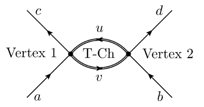
Figure 8: Overall T-channel. The vertex on the left side is labeled by number 1, the one on the right side by number 2.

The exclusion tables for the constraints at vertex 1 can be obtained by referring to Sec. 2.4:

$\textnormal{s-ch:}\;\;1\geq\left|\left(\tilde{a}-\tilde{v}\right)^{2}\right|=\left|\left(\tilde{c}-\tilde{u}\right)^{2}\right|\rightarrow\>$ X X X $\,,$

$\textnormal{t-ch:}\;\;1\geq\left|\left(\tilde{a}-\tilde{c}\right)^{2}\right|=\left|\left(\tilde{v}-\tilde{u}\right)^{2}\right|\rightarrow\>$ X X $\,,$

$\textnormal{u-ch:}\;\;1\geq\left|\left(\tilde{a}+\tilde{u}\right)^{2}\right|=\left|\left(\tilde{v}+\tilde{c}\right)^{2}\right|\rightarrow\>$ X X X $\,.$

The constraints at vertex 2 read:

$\textnormal{s-ch:}\;\;1\geq\left|\left(\tilde{v}+\tilde{b}\right)^{2}\right|=\left|\left(\tilde{u}+\tilde{d}\right)^{2}\right|\rightarrow\>$ X X X $\,,$

$\textnormal{t-ch:}\;\;1\geq\left|\left(\tilde{v}-\tilde{u}\right)^{2}\right|=\left|\left(\tilde{b}-\tilde{d}\right)^{2}\right|\rightarrow\>$ X X $\,,$

$\textnormal{u-ch:}\;\;1\geq\left|\left(\tilde{v}-\tilde{d}\right)^{2}\right|=\left|\left(\tilde{b}-\tilde{u}\right)^{2}\right|\rightarrow\>$ X X X $\,.$

In analogy to Sec. 3.1, we superimpose all combinations of the tables for the two vertices to obtain the result shown in Tab. 2.

		s-ch.			t-ch.			u-ch.
s- ch.		X	X		X	X		X	X
		X	X		X			X
t-ch.			X			X		X	X
		X	X		X			X
u-ch.			X			X		X	X
		X	X		X	X		X	X

Table 2: Forbidden combinations of energy flow in all scattering-channel combinations of the overall T-channel (and U-channel) by momentum transfer constraints.

That is, for the overall T-channel (or for the overall U-channel) eight possible configurations cannot yet be eliminated.

3.4 Exclusion of t-channels in the overall T-channel

The same argumentation that excluded the combination Sss in Chapter 3.2, relying on a momentum transfer constraint, energy momentum conservation, and on the on-shellness of the loop modes, exclude the combinations Tts, Ttt, Ttu, Tst and Tut. Thus, we obtain an updated version of the exclusion Tab. 2 in terms of Tab. 3.

		s-ch.			t-ch.			u-ch.
s- ch.		X	X		X	X		X	X
		X	X		X	X
t-ch.		X	X		X	X		X	X
		X	X		X	X		X	X
u-ch.					X	X		X	X
		X	X		X	X		X	X

Table 3: Forbidden combinations of energy flow in all scattering-channel combinations of the overall T-channel (and U-channel) by momentum transfer constraints and energy momentum conservation.

Again, only four configurations are left unexcluded.

3.5 Monte-Carlo analysis of remaining cases

For 4 out of the 36 configurations in each of the overall S-, T-, and U-channels no analytical exclusion could be performed. These remaining cases thus are treated numerically. To obtain an estimate on numerical precision in sampling the according algebraic varieties in these non-excluded combinations we also sample the analytically excluded Sss configuration. To proceed, a suitable set of non-redundant variables must be defined. As we will see, it is possible to parametrize the overall scattering process by the variables (referring to Fig. 6) $a_{0}$, $b_{0}$, the energies of the incoming photons, the angle $\alpha\equiv\measuredangle\mathbf{a}\mathbf{b}\in\left[0,2\pi\right]$ between their three-momenta, and the angles $\zeta\in\left[-\frac{\pi}{2},\frac{\pi}{2}\right]$ and $\eta\in\left[0,2\pi\right]$, that are necessary to describe the spatial orientation of one of the outgoing particles. Moreover two angles, $\theta\in\left[-\frac{\pi}{2},\frac{\pi}{2}\right]$ and $\varphi\in\left[0,2\pi\right]$, are sufficient to describe the kinematic state of the internal particles.

 

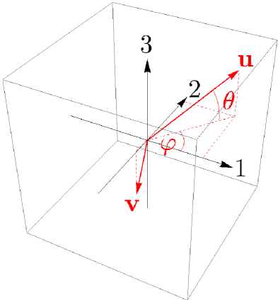
Figure 9: A visualization of the involved three-momenta (redundant variables). The incoming momenta are blue, the internal ones are red, and the outgoing momenta are green.

In the following we relate the involved four-momenta with respect to these parameters. First, we exploit four-momentum conservation and that the external photons are on shell:

$$a=\left(\begin{array}[]{c}a_{0}\\ a_{0}\\ 0\\ 0\end{array}\right)\>,\>b=\left(\begin{array}[]{c}b_{0}\\ b_{0}\cos\left(\alpha\right)\\ b_{0}\sin\left(\alpha\right)\\ 0\end{array}\right)\>,\>c=\left(\begin{array}[]{c}c_{0}\\ c_{0}\cos\left(\zeta\right)\cos\left(\eta\right)\\ c_{0}\cos\left(\zeta\right)\sin\left(\eta\right)\\ c_{0}\sin\left(\zeta\right)\end{array}\right)\>,\>d=a+b-c$$ (69)

Eq. (69) implies

$$0=d^{2}=\left(a+b-c\right)^{2}=2ab-2ac-2bc$$

$$\phantom{0}=2\left(a_{0}b_{0}-\left(a_{0}+b_{0}\right)c_{0}-a_{0}b_{0}\cos\left(\alpha\right)+c_{0}\left(b_{0}\cos\left(\alpha-\eta\right)+a_{0}\cos\left(\eta\right)\right)\sin\left(\zeta\right)\right)$$

$$\Rightarrow c_{0}=\frac{a_{0}b_{0}(1-\cos(\alpha))}{a_{0}+b_{0}-b_{0}\cos\left(\alpha-\eta\right)\sin\left(\zeta\right)-a_{0}\cos\left(\eta\right)\sin\left(\zeta\right)}\,,$$

independently of the overall scattering channel S, T, or U. Momenta of the massive modes, however, are dependent on S, T, or U. Both internal particles are on shell. For the overall S-channel and for given incoming momenta $\tilde{a},\tilde{b}$ the absolute value of loop three-momentum $\left|\mathbf{u}\right|$ is related to its orientation $\mathbf{e_{u}}$, which depends on $\theta$ and $\varphi$, as given in Eq. (50). We have

$$\left|\mathbf{\tilde{u}}\right|_{1/2}^{S}= \frac{\left(\tilde{a}\tilde{b}\right)\left(\mathbf{\tilde{a}}+\mathbf{\tilde{b}}\right)\mathbf{e_{u}}}{\left(\tilde{a}_{0}+\tilde{b}_{0}\right)^{2}-2\left(\left(\mathbf{\tilde{a}}+\mathbf{\tilde{b}}\right)\mathbf{e_{u}}\right)^{2}}$$

$$\pm\frac{\left(\tilde{a}_{0}+\tilde{b}_{0}\right)\sqrt{-\tilde{m}^{2}\left(\tilde{a}_{0}+\tilde{b}_{0}\right)^{2}+\left(\tilde{a}\tilde{b}\right)^{2}+\tilde{m}^{2}\left(\left(\mathbf{\tilde{a}}+\mathbf{\tilde{b}}\right)\mathbf{e_{u}}\right)^{2}}}{\left(\tilde{a}_{0}+\tilde{b}_{0}\right)^{2}-\left(\left(\mathbf{\tilde{a}}+\mathbf{\tilde{b}}\right)\mathbf{e_{u}}\right)^{2}}\,.$$ (70)

The expressions for the overall T- and U-channels can be obtained by interchanging momenta: The T-channel relates to the S-channel by exchanging $a\rightarrow c$ and $b\rightarrow-a$; the U-channel relates to the S-channel by $a\rightarrow d$ and $b\rightarrow-a$. Clearly, the energy $u_{0}$ is determined by on-shellness, and the other internal four-momentum $\tilde{v}$ is completely determined by four-momentum conservation. Whether or not a given set of parameter values satisfies all constraints is tested by inserting it into Eqs. (69) and (70) before, in turn, the 4-vertex constraints are probed at a given value of the dimensionless temperature $\lambda$. Because $\lambda$, $a_{0}$, $b_{0}$ are not bounded from above their to-be-tested values need to be limited in the numerical procedure. We require $\lambda_{c}=13.867\leq\lambda\leq 100$ [8] and $\hat{a}_{0}=\frac{a_{0}}{T}$, $\hat{b}_{0}=\frac{b_{0}}{T}\leq 100$. Here $\lambda_{c}$ is the critical temperature for the deconfining-preconfining phase transition where $m\to\infty$ and massive modes thus decouple.

Parameter values are sampled randomly in a conditioned way, and parameter sets satisfying the constraints are counted (for detailed information, see Appendix 5).

3.5.1 Typical hit densities

In the overall S channel, 87 out of $6.144\times 10^{10}$ tested parameter sets satisfied the constraints. This number is suppressed by a factor $\sim$ thirteen compared to the overall T-channel where $1110$ out of $6.144\times 10^{10}$ sets satisfied the constraints. Because of the afore mentioned symmetry of the constraints under the exchange of outgoing photons T- and U-channel should yield identical results. The number quoted for the T-chanell represents the average of all four remaining combinations in Tsu and Tus. We conclude from the S- versus T- plus U- channel comparison that the former is supported by less than 5% of the integration volume of the latter two channels. Practically, this excludes the overall S-channel. We also investigated the distribution of valid parameter values. For example, Fig. 10 depicts the abundance of the sum of hits over all non-excluded channel combinations as a function of $\lambda$.

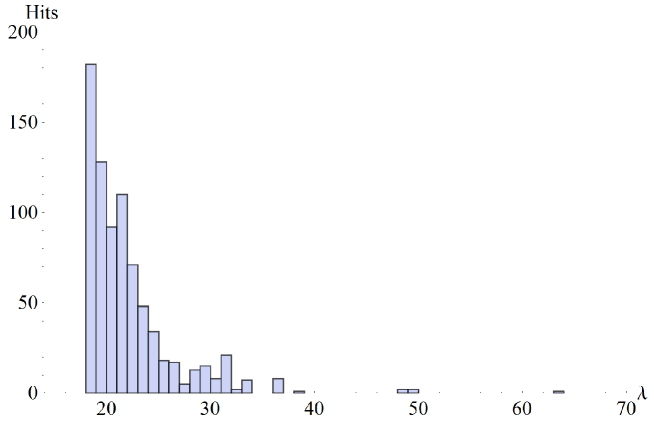
Figure 10: This histogram shows the distribution of the sum of hits over all tested channel combinations as a function of dimensionless temperature $\lambda$ in the range from $\lambda_{c}=13.867$ to $100$.

Two things are worth pointing out. First, we see that processes with $\lambda>40$ are very rare. The highest temperature associated with a valid configuration is $\lambda=63.32$, and this is an extreme outlier. Second, the abundance is rapidly decaying for $\lambda\leq 18.8$. In fact, a contribution at a temperature smaller than $\lambda=18.15$ never was detected.

Another interesting distribution is the abundance of energies relative to temperature $T$, $\hat{a}_{0}$ and $\hat{b}_{0}$, as shown in Fig. 11. As anticipated, there is no obvious difference between the distributions of $\hat{a}_{0}$ and $\hat{b}_{0}$. The constraints seem to imply an upper bound of about $40$. Configurations with values of $\hat{a}_{0}$ and $\hat{b}_{0}$ above this bound are anyway strongly suppressed by the Bose-Einstein distributions associated with external, thermalized photons.

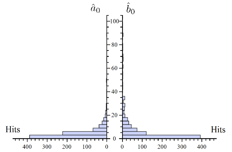
Figure 11: Comparison of the distributions of the two incoming energies, normalized with respect to temperature $T$. Hits in each bin represent the sum over all tested channel combinations.

3.5.2 Algebraic varieties

To explore the numerical data further, we zoom into the $\theta$-$\varphi$ plane about valid parameter-value combinations ($\lambda\mbox{, }\alpha\mbox{, }\beta\mbox{, }\gamma\mbox{, }\tilde{a}_{0}\mbox{ and }\tilde{b}_{0}$). It was numerically not possible to resolve the associated varieties of valid configuration about a particular one at once. Therefore we imposed a relaxation of the constraints to broaden the region of valid configurations. The relaxation is implemented by virtue of a softening factor $\Upsilon$ implemented as $1\rightarrow\Upsilon$ on the right hand sides in Eqs. (31) to (36). (The momentum transfer must only be smaller than $\Upsilon\left|\phi\right|^{2}$ in the relaxed as opposed to the physical situation.) For the combination shown in Fig. 13, representative of all other non-excluded combinations, there are series of four region plots. The first (top left) depicts a region of interest of size $\Delta\theta=0.4$ and $\Delta\varphi=0.8$ which is centered around the pivotal hit detected during the Monte Carlo test. This region is blown up into the second plot (top right) where, in turn, a centered region of interest of size $\Delta\theta=0.04$ and $\Delta\varphi=0.08$ is shown. Again, the latter is blown up into the third region plot (bottom left). The region of interest marked here and shown in full size in plot four (bottom right) has an extent of $\Delta\theta=0.004$ and $\Delta\varphi=0.008$. This last plot (lower right) represents the physical situation with $\Upsilon=1$. Values of the softening factor $\Upsilon$ are chosen to point out the nature of the actual, physical variety. We need to distinguish the two realizations for each channel combination (corresponding to the $\pm$ in the expression for $\left|\mathbf{u}\right|$ in Eq. (70)). The solution corresponding to $+$ is labeled by the index $1$, and the solution corresponding to the minus sign has the index $2$. The contour plots in the $\theta$-$\varphi$ plane signal the different constraints by a color code as explained in the caption of Fig. 12.

Figure 12: This region plot depicts color coded representations of the effects of single and combined constraints. The varieties marked in orange are associated with real and positive solutions $\left|\mathbf{u}\right|$ to Eq. (70). Varieties, where the momentum transfer constraints in the first vertex are satisfied, are marked in green, and those, where the momentum transfer constraints are fulfilled at the second vertex, are indicated in blue. The finally valid variety is represented by the intersection of these three varieties.

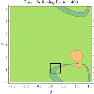
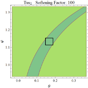
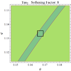
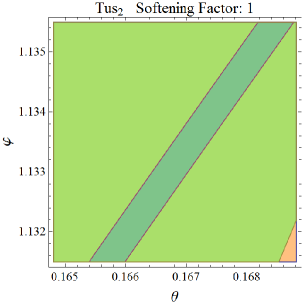
Figure 13: A visualization of the constraints in the $\theta$-$\varphi$ plane in the overall T-channel with scattering channels u and s for $\mbox{$\left|\mathbf{u}\right|$}_{2}$ and the following parameter values of the pivotal configuration: $\lambda=25.727$, $\tilde{a}_{0}=36.5239$, $\tilde{b}_{0}=11.0003$, $\alpha=1.53077$, $\eta=5.82265$, $\zeta=2.09548$.

4 Summary and Conclusions

In the present work we have discussed the nature of non-thermalities in SU(2) Yang-Mills theory, defined by a functional integral involving periodic gauge-field configurations. While the plane-wave sector behaves entirely thermal, it is the sector of isolatedly acting topological field configurations, which bears the seed of non-thermal behavior. Furthermore, we have investigated systematically how the unitary-gauge constraints of the effective theory for deconfining SU(2) Yang-Mills thermodynamics limit the contributions of loop momenta to the amplitude for one-loop photon-photon scattering. Only one type of Feynman diagrams with two 4-vertices is admissible to mediate this process, and a large part of channel and energy-sign combinations for the scattering through these vertices is analytically excluded relying on a subset of all energy-flow and momentum-transfer constraints. Out of a total of 108 scattering-channel and energy-sign configurations for the internal modes 12 configurations cannot be excluded analytically. These remaining cases do not give rise to pair creation or annihilation (practically, there is an exclusion of the overall S-channel) and were analyzed by Monte-Carlo sampling subject to all constraints. The associated hit densities decay very rapidly with temperature. We have also investigated the admissible algebraic variety in the vicinity of a selected, pivotal Monte-Carlo hit to demonstrate how filamentous it is.

One may, at first sight, object that an analysis of allowed regions for the loop integration is not sufficient to draw a conclusion about the actual smallness of the integral for the amplitude since singular integrands may arise on the filamentous integration regions. This is not the case, however, because we consider a reduced integration manifold, obtained after singular distributions in the original integrand are integrated out. (On-shell conditions, associated with $\delta$-distributions in the full 4$l$-dimensional space of loop integration at loop order $l$, are implemented in the analysis of vertex conditions from the start. Thus the integration manifold considered here is lower dimensional than 4$l$. Integrands are either regular, or if singular, thanks to their integrability can be made regular by non-singular changes of variables.)

All in all, our results suggest that photon-photon scattering within the deconfining SU(2) Yang-Mills plasma is feeble: Practically, it does not occur in the overall S-channel, excluding the creation of massive modes out of photons and vice versa by the optical theorem. This is in agreement with experiment.

Low-temperatures modification in thermal photon propagation from conventional U(1) behaviour, which could explain the large-angle anomalies of observed temperature fluctuations in the Cosmic Microwave Background [27], is largely dominated by the photon polarisation tensor. However, it is well possible that the feeble one-loop photon-photon correlation introduced by photon-photon scattering at low temperatures affects the Cosmic Microwave Background’s polarisation at low redshift (the domain of loop integration represents less than $10^{-7}$ times the volume of the unconstrained integration region). More work is required to actually match this to observational results [28].

Finally, a higher dimensional generalization (more than two 4-vertices per diagram) of the technology of energy-flow exclusion developed in the present work may be key to proving the termination of the expansion of thermodynamical quantities into irreducible bubble diagrams at a finite loop order, conjectured in [29] and based on a counting of constraints versus independent radial loop variables in dependence of loop order.

5 Appendix

Here we sketch the sampling strategy referred to in Sec. 3.5. Because we would like to do justice to the different scales of the sampling ranges and since runtime resources were limited we nested the sampling of random variables and required that noncompact variables are tested much more often than compact ones. The algorithm is sketched below in terms of a pseudocode:
 
repeat 60 times:

      $\lambda=$ random real number $\in\left[13.867,100\right]$;

      repeat 4 times:

            $\alpha=$ random real $\in\left[0,2\pi\right]$;

            repeat 4 times:

                  $\eta=$ random real $\in\left[0,2\pi\right]$;

                  repeat 2 times:

                        $\zeta=$ random real $\in\left[-\frac{\pi}{2},\frac{\pi}{2}\right]$;

                        repeat 2 times:

                              $\theta=$ random real $\in\left[-\frac{\pi}{2},\frac{\pi}{2}\right]$;

                              repeat 4 times:

                                    $\varphi=$ random real $\in\left[0,2\pi\right]$;

                                    repeat $10^{4}$ times:

                                          $\hat{a}_{0}=$ random real $\in\left[0,100\right]$;

                                          $\hat{b}_{0}=$ random real $\in\left[0,100\right]$;

                                          test if constraints for given channel-combination

                                           are satisfied for the given parameters

                                          $\lambda$, $\hat{a}_{0}$, $\hat{b}_{0}$, $\alpha$, $\eta$, $\zeta$, $\theta$, $\varphi$;

                                          if yes:

                                                increase hitcount by one;

                                                save parameters;

References

- [1] A. A. Belavin, A. M. Polyakov, A. S. Shvarts, and Yu. S. Tyupkin, Phys. Lett. B, 59, 85 (1975).
- [2] R. Jackiw and C. Rebbi, Phys. Rev. D 14, 517 (1976).
- [3] G. ’t Hooft, Phys. Rev. D 14, 3432 (1976); Erratum-ibid. Phys. Rev. D 18, 2199 (1978).
- [4] G. ’t Hooft, Phys. Rev. Lett. 37, 8 (1976).
- [5] R. Hofmann and D. Kaviani, Quant. Matt. 1, 41 (2012) [arXiv:1204.4112].
- [6] R. Hofmann, AIP Conf. Proc. 1479, 549 (2012) [arXiv:1210.2937].
- [7] U. Herbst and R. Hofmann, ISRN High Energy Phys. 2012, 373121 (2012) [arXiv:hep-th/0411214].
- [8] R. Hofmann, Int. J. Mod. Phys. A 20, 4123 (2005), Erratum-ibid. A 21, 6515 (2006) [arXiv:hep-th/0504064].
- [9] R. P. Feynman, Phys. Rev. 91, 1291 (1953).
- [10] R. P. Feynman and A. R. Hibbs, Quantum Mechanics and Path Integrals (McGraw-Hill) (1965).
- [11] S. Migdal, Paradise lost, in Continuous Advances in QCD 2006, eds. M. Peloso and M. Shifman (World Scientific Publishing Co. Pte. Ltd.) (2006).
- [12] D. Diakonov et al., Phys. Rev. D 70, 036003 (2004).
- [13] J. Ludescher, J. Keller, F. Giacosa, and R. Hofmann, Ann. Phys.19, 102 (2010).
- [14] B. J. Harrington and H. K. Shepard, Phys. Rev. D 17, 2122 (1978).
-
[15]
W. Nahm, Phys. Lett. B 90, 413 (1980).
W. Nahm, All self-dual multimonopoles for arbitrary gauge groups, CERN preprint TH-3172, (1981),
W. Nahm, Self-dual monopoles and calorons in Trieste Group Theor. Method 1983, p. 189, (1983). -
[16]
T. C. Kraan and P. Van Baal, Phys.
Lett. B 428, 268 (1998) [hep-th/9802049],
T. C. Kraan and P. Van Baal, Nucl. Phys. B 533, 627 (1998) [hep-th/9805168]. - [17] K. Lee and C. Lu, Phys. Rev. D 58, 025011-1 (1998) [hep-th/9802108].
- [18] R. Hofmann, The thermodynamics of Quantum Yang-Mills theory: Theory and Applications (Word Scientific, Singapore) (2012).
- [19] S. J. Brodsky and P. Hoyer, Phys. Rev. D 83, 045026 (2011) [arXiv:1009.2313].
- [20] R. Hofmann, arXiv:0710.0962.
- [21] M. Schwarz, R. Hofmann, and F. Giacosa, Int. J. Mod. Phys. A 22, 1213 (2007) [hep-th/0603078].
- [22] J. Ludescher and R. Hofmann, Ann. Phys. 18, 271 (2009) [arXiv:0806.0972].
- [23] C. Falquez and R. Hofmann, arXiv:1009.1715 [hep-th].
-
[24]
G. ’t Hooft and M. J. G. Veltman, Nucl.
Phys. B 44, 189 (1972),
G. ’t Hooft, Nucl. Phys. B 33, 173 (1971),
G. ’t Hooft, Nucl. Phys. B 62, 444 (1973),
G. ’t Hooft and M. J. G. Veltman, Nucl. Phys. B 50, 318 (1972). -
[25]
B. W. Lee and Jean Zinn-Justin, Phys.Rev.D 5,
3121 (1972),
B. W. Lee and Jean Zinn-Justin, Phys. Rev. D 5, 3137 (1972),
B. W. Lee and Jean Zinn-Justin, Phys. Rev. D 5, 3155 (1972). - [26] N. Krasowski, Kinematic constraints and their effects on photon-photon scattering in deconfining SU(2) Yang-Mills Thermodynamics, Master Thesis, Universität Heidelberg (2012).
- [27] R. Hofmann, Nature Physics 9 (11), 686 (2013).
- [28] P. A. R. Ade et al., arXiv:1404.3985.
- [29] R. Hofmann, Braz. J. Phys. 42, 110 (2012) [hep-th/0609033].