Spin-orbit-induced bound state and molecular signature of the degenerate Fermi gas in a narrow Feshbach resonance

Abstract

In this paper we explore the spin-orbit-induced bound state and molecular signature of the degenerate Fermi gas in a narrow Feshbach resonance based on a generalized two-channel model. Without the atom-atom interactions, only one bound state can be found even if spin-orbit coupling exists. Moreover, the corresponding bound-state energy depends strongly on the strength of spin-orbit coupling, but is influenced slightly by its type. In addition, we find that when increasing the strength of spin-orbit coupling, the critical point at which the molecular fraction vanishes shifts from zero to the negative detuning. In the weak spin-orbit coupling, this shifting is proportional to the square of its strength. Finally, we also show that the molecular fraction can be well controlled by spin-orbit coupling.

I Introduction

Recently, the investigation of spin-orbit (SO) coupling in neutral atoms has attracted much attentions JR . In particular, a one-dimensional (1D) equal Rashba and Dresselhaus SO coupling has been first realized in the ultracold ⁸⁷Rb atoms by a couple of Raman lasers Lin . By applying the same laser technique, this 1D SO coupling has been also achieved experimentally in the degenerate Fermi gas with ⁴⁰K PW and ⁶Li LWC . Theoretical investigations have been revealed that in the presence of SO coupling, the degenerate Fermi gas can exhibit the interesting physics in both three JPV ; GM ; YZQ ; HH ; JPV1 ; Iskin ; LJ ; WY1 ; LD ; Li ; KS ; KZ ; RL ; ZhangP1 ; Peng1 ; HLY1 ; LD1 and lower dimensions Chen ; MG ; HLY2 ; JZ ; WY2 ; XYang ; ZJN ; FW . For example, by increasing the strength of SO coupling, the density of state at the Fermi surface is increased, and the Cooper paring gap can be thus enhanced significantly GM ; YZQ ; HH . More importantly, this system may be changed from the Bardeen-Cooper-Schrieffer (BCS) superfluid to the Bose-Einstein condensate (BEC) with a new two-body bound state called Rashbon JPV ; HH . When an effective Zeeman field is applied, the 2D degenerate Fermi gas with the Rashba SO coupling exhibits an exotic topological superfluid supporting the Majorana fermions MG , which is the heart for realizing the topological quantum computing CN . Recently, a universal midgap bound state in the topological superfluid has been predicted HH1 .

To illustrate the SO-driven fundamental physics, a generalized one-channel model has been introduced in all previous considerations JPV ; GM ; YZQ ; HH ; JPV1 ; Iskin ; LJ ; WY1 ; LD ; Li ; KS ; KZ ; RL ; ZhangP1 ; Peng1 ; HLY1 ; LD1 ; Chen ; MG ; HLY2 ; JZ ; WY2 ; XYang ; ZJN ; FW . In this one-channel model, only the atoms tuned via the Feshbash-resonant technique are taken into account. However, it is valid for the broad Feshbash-resonant regime with $\Gamma\gg 1$ DES , where the dimensionless parameter is defined as $\Gamma=\sqrt{32m\mu_{\text{B}}a_{\text{bg}}^{2}B_{\text{w}}^{2}/(\hbar^{2}\pi E_{\text{F}})}$, $\mu_{\text{B}}$ is the Bohr magneton, $m$ is the atom mass, $a_{\text{bg}}$ is the background $s$-wave scattering strength, $B_{\text{w}}$ is the resonant width and $E_{\text{F}}$ is the Fermi energy. In fact, to get a more realistic and complete description of the degenerate Fermi gas, especially in the narrow Feshbash-resonant limit with $\Gamma\ll 1$, we must introduce a two-channel model MH ; ETI ; YO ; RDU ; Peng2 , which includes both the atoms in the open channel and the molecules in the closed channel. Moreover, in the narrow Feshbash-resonant regime, some fundamental properties can be observed experimentally by detecting the striking molecular signature GBP , additional to measuring the superfluid pairing gap applied usually in the one-channel model Chin2004 ; Shin ; STG . More importantly, new quantum phase transitions have been predicted YN ; ZS , attributed to the existence of extra U(1) symmetry for the molecular field. On the experimental side, the degenerate Fermi gas in the narrow Feshbach-resonant regime has been also reported successfully in ⁶Li ELH and the Fermi-Fermi mixture of ⁶Li and ⁴⁰K LC . Thus, it is crucially important to explore the SO-induced exotic physics in this regime JXC .

In the present paper we investigate the SO-induced bound state and molecular signature of the degenerate Fermi gas in the narrow Feshbach resonance. The main results are given as follows. (i) Without the atom-atom interactions, only one bound state can be found even if SO coupling exists. Moreover, the corresponding bound-state energy depends strongly on the strength of SO coupling, but is influenced slightly on its type. (ii) With the increasing of the strength of SO coupling, the critical point at which the molecular fraction vanishes shifts from zero to the negative detuning. In the weak SO coupling, this shifting is proportional to the square of its strength. (iii) Finally, we also show that the molecular fraction can be well controlled by SO coupling. We believe that in experiments it is a good signature to detect the SO-induced physics.

II Model and Hamiltonian

For the SO-driven two-channel model, the total Hamiltonian can be written formally as

$$H=H_{\text{F}}+H_{\text{M}}+H_{\text{I}}+H_{\text{S}}.$$ (1)

In Hamiltonian (1),

$$H_{\text{F}}=\sum_{\mathbf{k}\sigma}\epsilon_{\mathbf{k}}C_{\mathbf{k}\sigma}^{\dagger}C_{\mathbf{k}\sigma}$$ (2)

is the atom Hamiltonian, where $C_{\mathbf{k}\sigma}^{\dagger}$ is the creation operator for a atom with the momentum $\mathbf{k}$ and $\sigma=\uparrow,\downarrow$, and $\epsilon_{\mathbf{k}}=k^{2}/(2m)$ is the kinetic energy of the atom.

$$H_{\text{M}}=\sum_{\mathbf{q}}(\epsilon_{\mathbf{q}}+\delta_{0})b_{\mathbf{q}}^{\dagger}b_{\mathbf{q}}$$ (3)

is the molecular Hamiltonian, where $b_{\mathbf{q}}^{\dagger}$ is the creation operator of a molecule with the momentum $\mathbf{q}$, $\epsilon_{q}=\hbar^{2}q^{2}/(2M)$ with $M=2m$ is the kinetic energy of the molecule, and $\delta_{0}$ is the bare detuning determined by the Feshbash-resonant position $\delta$ via a relation

$$\delta_{0}=\delta+g^{2}\sum_{\mathbf{k}}\frac{1}{2\epsilon_{\mathbf{k}}}.$$ (4)

Without SO coupling, the system has the BCS superfluid in the positive detuning ($\delta>0$), and enters into the BEC regime in the negative detuning ($\delta<0$) MH ; ETI ; YO ; RDU ; Peng2 . At lower energy, the position is given approximately by $\delta\simeq 2\mu_{\text{B}}(B-B_{0})$, where $B_{0}$ is the magnetic field at which the resonance is at zero energy, and $B$ is the tunable magnetic field Chin . The atom-molecule interconversion term is governed by the following Hamiltonian

$$H_{\text{I}}=g\sum_{\mathbf{qkk}^{\prime}}b_{\mathbf{q}}^{\dagger}C_{-\mathbf{k}+\frac{\mathbf{q}}{2}\downarrow}C_{\mathbf{k}+\frac{\mathbf{q}}{2}\uparrow}+C_{\mathbf{k}^{\prime}+\frac{\mathbf{q}}{2}\uparrow}^{\dagger}C_{-\mathbf{k}^{\prime}+\frac{\mathbf{q}}{2}\downarrow}^{\dagger}b_{\mathbf{q}},$$ (5)

where $g$ is the coupling constant that measures the amplitude of the decay of the molecule in the closed channel into a pair of the open-channel atoms. Finally, the SO coupling is chosen as a generalized Rashba and Dresselhaus type. The corresponding Hamiltonian is given by

$$H_{\text{S}}=\alpha\sum_{\mathbf{k}}[(k_{y}+i\lambda k_{x})C_{\mathbf{k}\uparrow}^{\dagger}C_{\mathbf{k}\downarrow}+(k_{y}-i\lambda k_{x})C_{\mathbf{k}\downarrow}^{\dagger}C_{\mathbf{k}\uparrow}]$$ (6)

with $\alpha=(\alpha_{R}+\alpha_{D})$ and $\lambda=(\alpha_{R}-\alpha_{D})/(\alpha_{R}+\alpha_{D})$, where $\alpha_{R}$ and $\alpha_{D}$ are the SO coupling strengths for the Rashba and Dresselhaus types, respectively. Clearly, $\alpha$ is the generalized strength of SO coupling and the dimensionless parameter $\lambda\$reflects the competition between these different types of SO coupling. For example, for $\lambda=1$ ($\alpha_{D}=0$), the 2D Rashba SO coupling can be found. Whereas, for $\lambda=0$ ($\alpha_{D}=\alpha_{R}$), the 1D equal Rashba and Dresselhaus SO coupling can be generated. Fortunately, this 1D SO coupling has been realized experimentally in the ultracold neutral atoms Lin ; PW ; LWC .

In the absence of SO coupling, the limit $\mathbf{q=0}$ can be applied usually to discuss the standard two-channel model including the effective Zeeman field DES . However, in the presence of SO coupling, the result is quite complicated. If both SO coupling and the effective Zeeman field are taken into account, the parity and time-reversal symmetries are broken. As a result, the $\mathbf{q}$-dependent order parameter should be introduced DFA . However, in this paper we do not consider the effect of the effective Zeeman field and thus may focus on the case of $\mathbf{q=0}$.

III Two-body bound state

We begin to discuss the two-body bound state of the generalized two-channel model (1) by introducing the ansatz wavefunction. In the absence of SO coupling ($\alpha=0$), Hamiltonian (1) reduces to the standard two-channel model $H=\sum_{\mathbf{k}\sigma}\xi_{\mathbf{k}}C_{\mathbf{k}\sigma}^{\dagger}C_{\mathbf{k}\sigma}+\sum(\delta_{0}-2\mu)b_{0}^{\dagger}b_{0}+g\sum_{\mathbf{kk}^{\prime}}b_{0}^{\dagger}C_{-\mathbf{k}\downarrow}C_{\mathbf{k}\uparrow}+C_{\mathbf{k}^{\prime}\uparrow}^{\dagger}C_{-\mathbf{k}^{\prime}\downarrow}^{\dagger}b_{0}$ MH ; ETI ; YO ; RDU , in which only the singlet Cooper paring can be formed. However, in the presence of SO coupling, both the singlet and triplet Cooper parings can coexist LPG . As a result, the ansatz wavefunction should be written formally as

$$\left|\Psi\right\rangle=(\sum_{k^{{}^{\prime}}\sigma\sigma^{{}^{\prime}}}\beta_{k^{{}^{\prime}}\sigma\sigma^{{}^{\prime}}}C_{\mathbf{k}^{\prime}\sigma}^{\dagger}C_{\mathbf{k}^{\prime}\sigma^{{}^{\prime}}}^{\dagger}+\gamma b_{0}^{\dagger})\left|0,0,0,0\right\rangle\otimes\left|0\right\rangle,$$ (7)

where $\beta_{k^{{}^{\prime}}\uparrow\downarrow}$ and $\beta_{k^{{}^{\prime}}\downarrow\uparrow}$ ($\beta_{k^{{}^{\prime}}\uparrow\uparrow}$ and $\beta_{k^{{}^{\prime}}\downarrow\downarrow}$) represent the probability amplitude of the singlet (triplet) Cooper paring, $\gamma$ stands for the  probability amplitude of the molecule, and $\left|0,0,0,0\right\rangle\otimes\left|0\right\rangle$ is the direct multiple of the fermion vacuum with spin flipping and the molecule vacuum. Substituting the wavefunction in Eq. (7) into the stationary Schrödinger equation

$$(H-E)\left|\Psi\right\rangle=0,$$ (8)

we find that the six coefficients determining the ansatz wavefunction $\left|\Psi\right\rangle$ and the energy $E$ are governed by the following equations:

$$\left\{\begin{array}[]{c}g\gamma+\beta_{k^{{}^{\prime}}\uparrow\uparrow}\alpha k_{-}=\Xi_{k}\beta_{k\downarrow\uparrow}\\ g\gamma+\beta_{k^{{}^{\prime}}\downarrow\downarrow}\alpha k_{+}=\Xi_{k}\beta_{k\uparrow\downarrow}\\ (\beta_{k^{{}^{\prime}}\downarrow\uparrow}+\beta_{k^{{}^{\prime}}\uparrow\downarrow})\alpha k_{+}=\Xi_{k}\beta_{k^{{}^{\prime}}\uparrow\uparrow}\\ (\beta_{k^{{}^{\prime}}\downarrow\uparrow}+\beta_{k^{{}^{\prime}}\uparrow\downarrow})\alpha k_{-}=\Xi_{k}\beta_{k^{{}^{\prime}}\downarrow\downarrow}\\ 2(\delta_{0}-E)\gamma=-g\sum_{k^{{}^{\prime}}}(\beta_{k^{{}^{\prime}}\uparrow\downarrow}+\beta_{k^{{}^{\prime}}\downarrow\uparrow})\end{array}\right.,$$ (9)

where $\Xi_{k}=E-2\epsilon_{k}$ and $k_{\pm}=k_{y}\pm i\lambda k_{x}$. Eq. (9) can not be solved directly because of lack of a coefficient equation. If we define the spin symmetry and anti-symmetry vectors as

$$\left\{\begin{array}[]{c}\psi_{s}(k)=\frac{1}{\sqrt{2}}(\beta_{k\downarrow\uparrow}-\beta_{k\uparrow\downarrow})\\ \psi_{a}(k)=\frac{1}{\sqrt{2}}(\beta_{k\downarrow\uparrow}+\beta_{k\uparrow\downarrow})\end{array}\right.,$$ (10)

the stationary Schrödinger equation is rewritten as $(H-E)\psi_{k}=0$ in the representation of $\psi_{k}=[\beta_{k\uparrow\downarrow},\beta_{k\downarrow\uparrow},\beta_{k\downarrow\downarrow},\beta_{k\uparrow\uparrow},\gamma]^{T}$. This leads to another equations for the coefficients $\beta_{k^{{}^{\prime}}\sigma,\sigma^{{}^{\prime}}}$ and $\gamma$, that is,

$$\left\{\begin{array}[]{c}\gamma=-\sum_{k^{{}^{\prime}}}\frac{g\sqrt{2}\psi_{a}(k^{{}^{\prime}})}{(\delta_{0}-E)}\\ \beta_{k^{{}^{\prime}}\uparrow\uparrow}=\frac{\sqrt{2}\psi_{a}(k)\alpha k_{+}}{\Xi_{k}}\\ \beta_{k^{{}^{\prime}}\downarrow\downarrow}=\frac{\sqrt{2}\psi_{a}(k)\alpha k_{-}}{\Xi_{k}}\end{array}\right..$$ (11)

Substituting Eq. (11) into Eq. (9) yields

$$\sum_{k}(\frac{\Xi_{k}}{\Xi_{k}^{2}-4\alpha^{2}k_{+}k_{-}}+\frac{1}{2\epsilon_{k}})=\frac{E-\delta}{g^{2}}.$$ (12)

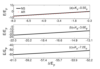
Figure 1: (Color online) The bound-state energy for the 2D Rashba SO coupling ($\lambda=1$) as a function of the detuning $\delta$ for the different strengths of SO coupling (a) $\alpha K_{\text{F}}=0.5E_{\text{F}}$, (b) $\alpha K_{\text{F}}=3.6E_{\text{F}}$, and (c) $\alpha K_{\text{F}}=7.2E_{\text{F}}$ when $\Gamma=0.1$. In Fig. 1(a), the red open symbol corresponds to the analytical result (AR) and the black solid line represents the direct numerical simulation (NS).

Equation (12), which is the main result of this paper, determines the SO-induced bound-state energy of the generalized two-channel model (1). The procedure is given as follows. (i) We first obtain the energy $E$ from Eq. (12). (ii) Then, we introduce the threshold energy $E_{T}$, which is the lowest energy of the free particle (i.e., the lowest band), to judge whether this energy is the bound-state energy or not. If $E<E_{T}$, the bound state exists and the corresponding energy $E$ is called the bound-state energy, and vice versa JPV . According to its definition, the threshold energy $E_{T}$ of the generalized two-channel model (1) is evaluated as

$$E_{T}=-\frac{2m\alpha^{2}}{\hbar^{2}}.$$ (13)

In the absence of SO coupling ($\alpha=0$), this threshold energy becomes $E_{T}=0$, as expected. In the following discussions, we mainly consider two interesting cases, including the 2D Rashba SO coupling ($\lambda=1$) and 1D equal Rashba and Dresselhaus SO coupling ($\lambda=0$), to reveal the fundamental properties of the bound state.

We first address the case of the 2D Rashba SO coupling ($\lambda=1$). In the absence of SO coupling ($\alpha=0$), the analytical bound-state energy is derived from Eq. (12) by

$$E=\frac{1}{32\pi^{2}\hbar^{6}}(-g^{4}m^{3}+32\pi^{2}\delta\hbar^{6}-g^{2}\sqrt{g^{4}m^{6}-64m^{3}\pi^{2}\delta\hbar^{6}}).$$ (14)

It implies that in such a case only one bound state can be found DES . In the presence of SO coupling ($\alpha\neq 0$), the explicit expression for the bound-state energy can not be obtained. However, for the weak SO coupling, Eq. (12) is simplified as

$$\frac{m^{\frac{3}{2}}[2\hbar^{2}E+(1+\lambda^{2})m\alpha^{2}]}{8\pi\hbar^{5}\sqrt{-E}}=\frac{E-\delta}{g^{2}}$$ (15)

with the help of a Taylor expansion with respect to the strength of SO coupling. In this case, Hamiltonian (1) also exhibits one bound state, as shown in Fig. 1(a). By further solving Eq. (15) approximately, we find that the bound-state energy is proportional to $-\alpha^{4}$. This behavior agrees well with the numerical simulation, as also shown in Fig. 1(a). It implies that the bound-state energy can decrease by increasing the strength of SO coupling. For the strong SO coupling, the perturbation method is invalid. Here we numerically solve Eq. (12) to evaluate the bound-state energy $E$. Even if the strong SO coupling exists, only one bound state can be found, as shown in Figs. 1(b) and 1(c)

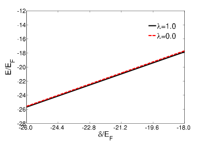
Figure 2: (Color online) The bound-state energy as a function of the detuning $\delta$ for the different types of SO coupling including $\lambda=1$ (the 2D Rashba SO coupling) and $\lambda=0$ (the 1D equal Rashba and Dresselhaus SO coupling) when $\Gamma=0.1$ and $\alpha K_{\text{F}}=4.2E_{\text{F}}$.

In Fig. 2, we plot the bound-state energy with respect to the detuning $\delta$ for the different types of SO coupling including $\lambda=1$ (the 2D Rashba SO coupling) and $\lambda=0$ (the 1D equal Rashba and Dresselhaus SO coupling). It can be seen clearly that the bound-state energy is affected slightly by the type of SO coupling.

When the Feshbach-resonant width parameter $\Gamma$ increases, the system changes from the narrow limit ($\Gamma\ll 1$) to the broad limit ($\Gamma\gg 1$). Especially, for the broad limit ($\Gamma\gg 1$), Eq. (12) becomes

$$\sum_{k}(\frac{\Xi_{k}}{\Xi_{k}^{2}-4\alpha^{2}k_{+}k_{-}}+\frac{1}{2\epsilon_{k}})\simeq-\frac{\delta}{g^{2}}=\frac{m}{4\pi\hbar^{2}a_{s}},$$ (16)

which is similar to the result of Ref. YZQ . In Fig. 3, we plot the bound-state energy for the 1D equal Rashba and Dresselhaus SO coupling as a function of the detuning $\delta$ for the different Feshbach-resonant width parameters (a) $\Gamma=0.1$, (b) $\Gamma=30.0$, and (c) $\Gamma=300.0$. This figure shows again that for the broad limit our considered two-channel model reduces to the single-channel model. However, it should be remarked that the energy $E$ for the broad Feshbach resonance is not a bound-state energy, but is a two-body interaction energy approaching infinitely the bound-state energy LDL

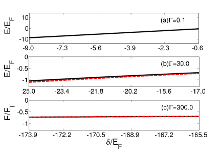
Figure 3: (Color online) The bound-state energy for the 1D equal Rashba and Dresselhaus SO coupling with $\lambda=0$ as a function of the detuning $\delta$ for the different Feshbach-resonant widths (a) $\Gamma=0.1$, (b) $\Gamma=30$, and (c) $\Gamma=300.0$ when $\alpha K_{F}=0.7E_{F}$. In (b) and (c), the red dash line corresponds to the numerical solution of Eq. (16). For the 2D Rashba SO coupling, the similar conclusion can be also found.

IV Molecular signature

Having obtained the bound-state energy in the generalized two-channel model, it is conveniently to discuss the experimentally-measurable molecular signature. In terms of the Hellmann-Feymann theorem, the molecular fraction is obtained by

$$N_{0}=\left\langle\Psi\right|b_{0}^{\dagger}b_{0}\left|\Psi\right\rangle=\left\langle\Psi\right|\frac{\partial H}{\partial\delta_{0}}\left|\Psi\right\rangle=\frac{dE}{d\delta},$$ (17)

where the bound-state energy $E$ can be derived from Eq. (12).

Figure 4 is plotted the scaled molecular fraction $2N_{0}/N$ of both the 2D Rashba SO coupling ($\lambda=1$) and the 1D equal Rashba and Dresselhaus SO coupling ($\lambda=0$) with respect to the detuning $\delta$ for the different strengths of SO coupling. In the absence of SO coupling ($\alpha=0$), the molecule exists in the negative detuning ($\delta<0$). However, for the positive detuning ($\delta\geq 0$), the physical bound state vanishes LDL , i.e., there is no real molecular fraction. With the increasing of the strength of SO coupling, the critical point at which the molecular fraction vanishes shifts from zero to the negative detuning. The physics can be understood as follows. In the generalized two-channel model, the molecules play two roles. One is that they interact directly with the atoms via Hamiltonian $H_{\text{I}}$. The other (the most important) is that they induce the indirect atom-atom interactions, which generate the Cooper pairing. When the Cooper pairing is enhanced by SO coupling GM ; YZQ ; HH , the molecules are thus suppressed because the system need guarantee a conserved number $N=2b_{0}^{\dagger}b_{0}+\sum_{\mathbf{k}\sigma}C_{\mathbf{k}\sigma}^{\dagger}C_{\mathbf{k}\sigma}$. In order to see clearly this behavior induced by SO coupling, we introduce a key parameter $\delta_{m}$. This parameter describes the maximum detuning at which the molecular fraction exists. In terms of the definition, the parameter $\delta_{m}$ is given by

$$\delta_{m}=-\frac{2m\alpha^{2}}{\hbar^{2}}-g^{2}[\sum_{k}(\frac{\Xi_{k}}{\Xi_{k}^{2}-4\alpha^{2}k_{+}k_{-}}+\frac{1}{2\epsilon_{k}})]_{E=E_{T}}.$$ (18)

In the case of the weak SO coupling, the parameter $\delta_{m}$ is obtained explicitly by

$$\delta_{m}=-\frac{32\hbar^{2}m\pi\alpha^{2}+\sqrt{2}g^{2}m^{2}(\lambda^{2}-3)\alpha}{16\pi\hbar^{4}}\simeq-\alpha^{2}.$$ (19)

Eq. (19) shows clearly that $\delta_{m}$ decreases with the increasing of the strength of SO coupling.

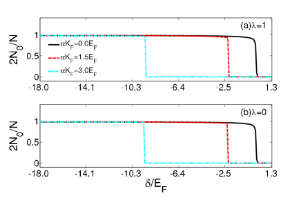
Figure 4: (Color online) The molecular fraction of both (a) the 2D Rashba SO coupling with $\lambda=1$ and (b) the 1D equal Rashba and Dresselhaus SO coupling with $\lambda=0$ as a function of the detuning $\delta$ for the different strengths of SO coupling when $\Gamma=0.1$.

In Fig. 5, we plot the molecular fraction of both the 2D Rashba SO coupling ($\lambda=1$) and the 1D equal Rashba and Dresselhaus SO coupling ($\lambda=0$) with respect to the strength of SO coupling for the different detunings. In the negative detuning ($\delta<\delta_{m}$) we shows again that the SO coupling suppresses the molecular fraction. With the increasing of the strength of SO coupling, the molecular fraction also vanishes. It means that in experiment the molecular fraction can be well controlled by tuning the SO strength. In addition, in the positive detuning, no molecular fraction can be found even if SO coupling exists.

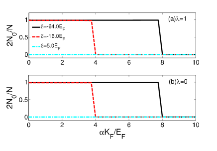
Figure 5: (Color online) The molecular fraction of both (a) the 2D Rashba SO coupling with $\lambda=1$ and (b) the 1D equal Rashba and Dresselhaus SO coupling with $\lambda=0$ as a function of the strength $\alpha K_{\text{F}}$ of SO coupling for the different detunings when $\Gamma=0.1$.

V Conclusions and Remarks

In summary, motivated by the recent experimental developments, we have investigated the SO-driven degenerate Fermi gas in the narrow Feshbash resonance based on the generalized two-channel model. We have found that in the absence of the atom-atom interactions, only one bound state can be found even if SO coupling exists. In addition, we have shown that the molecular fraction can be well controlled by SO coupling. We believe that in experiments it is a good signature to explore the SO-induced physics.

VI Acknowledgements

We thank Professors Peng Zhang, Wei Yi, Wei Zhang, Shizhong Zhang and Doctor Zengqiang Yu for their helpful discussions. This work was supported partly by the 973 program under Grant No. 2012CB921603; the NNSFC under Grants No. 10934004, No. 11074154, and No. 61275211; NNSFC Project for Excellent Research Team under Grant No. 61121064; and International Science and Technology Cooperation Program of China under Grant No.2001DFA12490.

Note added–During preparing this paper, we noticed that two bound states for the SO-driven two-channel model with the atom-atom interactions was predicted by V. B. Shenoy in terms of a renormalizable quantum field theory VBS1 . However, that paper does not consider the molecular fraction.

References

- (1) J. Dalibard, F. Gerbier, G. Juzeliūnas, and P. Öhberg, Rev. Mod. Phys. 83, 1523 (2011).
- (2) Y. -J. Lin, K. Jimenez-Garcia, and I. B. Spielman, Nature (London), 471, 83 (2011).
- (3) P. Wang, Z. -Q. Yu, Z. Fu, J. Miao, L. Huang, S. Chai, H. Zhai, and J. Zhang, Phys. Rev. Lett. 109, 095301 (2012).
- (4) L. W. Cheuk, A. T. Sommer, Z. Hadzibabic, T. Yefsah, W. S. Bakr, and M. W. Zwierlein, Phys. Rev. Lett. 109, 095302 (2012).
- (5) J. P. Vyasanakere and V. B. Shenoy, Phys. Rev. B 83, 094515 (2011).
- (6) M. Gong, S. Tewari, and C. Zhang, Phys. Rev. Lett. 107, 195303 (2011).
- (7) Z. -Q. Yu and H. Zhai, Phys. Rev. Lett. 107, 195305 (2011).
- (8) H. Hu, L. Jiang, X. -J. Liu, and H. Pu, Phys. Rev. Lett. 107, 195304 (2011).
- (9) J. P. Vyasanakere, S. Zhang, and V. B. Shenoy, Phys. Rev. B 84, 014512 (2011).
- (10) M. Iskin, and A. L. Subasi, Phys. Rev. Lett. 107, 050402 (2011); Phys. Rev. A 84, 043621 (2011).
- (11) L. Jiang, X. -J. Liu, H. Hu, and H. Pu, Phys. Rev. A 84, 063618 (2011).
- (12) W. Yi and G. -C. Guo, Phys. Rev. A 84, 031608 (2011).
- (13) L. Dell’Anna, G. Mazzarella, and L. Salasnich, Phys. Rev. A 84, 033633 (2011); Phys. Rev. A 86, 053632 (2012).
- (14) L. Han and C. A. R. Sá de Melo, Phys. Rev. A 85, 011606 (2012).
- (15) K. Seo, L. Han, and C. A. R. Sá de Melo, Phys. Rev. Lett. 109, 105303 (2012); Phys. Rev. A 85, 033601 (2012); arXiv:1301.1353 (2013).
- (16) K. Zhou and Z. Zhang, Phys. Rev. Lett. 108, 025301 (2012).
- (17) R. Liao, Y. -X. Yu, and W. -M. Liu, Phys. Rev. Lett. 108, 080406 (2012).
- (18) P. Zhang, L. Zhang, and Y. Deng, Phys. Rev. A 86, 053608 (2012); P. Zhang, L. Zhang, and W. Zhang, Phys. Rev. A 86, 042707 (2012).
- (19) S. -G. Peng, X. -J. Liu, H. Hu, and K. Jiang, Phys. Rev. A 86, 063610 (2012).
- (20) L. He and X. -G. Huang, Phys. Rev. B 86, 014511 (2012).
- (21) L. Dong, L. Jiang, H. Hu, and H. Pu, Phys. Rev. A 87, 043616 (2013).
- (22) G. Chen, M. Gong, and C. Zhang, Phys. Rev. A 85, 013601 (2012).
- (23) M. Gong, G. Chen, S. Jia, and C. Zhang, Phys. Rev. Lett. 109, 105302 (2012).
- (24) L. He and X. -G. Huang, Phys. Rev. Lett. 108, 145302 (2012); Phys. Rev. A 86, 043618 (2012).
- (25) J. Zhou, W. Zhang, and W. Yi, Phys. Rev. A 84, 063603 (2012).
- (26) W. Yi and W. Zhang, Phys. Rev. Lett. 109, 140402 (2012).
- (27) X. Yang and S. Wan, Phys. Rev. A 85, 023633 (2012).
- (28) J. -N. Zhang, Y. -H. Chan, and L. -M. Duan, arXiv:1110.2241 (2011).
- (29) F. Wu, G. -C. Guo, W. Zhang, and W. Yi, Phys. Rev. Lett. 110, 110401 (2013).
- (30) C. Nayak, S. H. Simon, A. Stern, M. Freedman, and S. Das Sarma, Rev. Mod. Phys. 80, 1083 (2008).
- (31) H. Hu, L. Jiang, H. Pu, Y. Chen, and X. -J. Liu, Phys. Rev. Lett. 110, 020401 (2013).
- (32) D. E. Sheehy and L. Radzihovsky, Phys. Rev. Lett. 96, 060401 (2006); Ann. Phys. 322, 1790 (2007).
- (33) M. Holland, S. J. J. M. F. Kokkelmans, M. L. Chiofalo, and R. Walser, Phys. Rev. Lett. 87, 120406 (2001).
- (34) E. Timmermans, K. Furuya, P. W. Milonni, and A. K. Kerman, Phys. Lett. A 285, 228 (2001).
- (35) Y. Ohashi and A. Griffin, Phys. Rev. Lett. 89, 130402 (2002).
- (36) R. Duine and H. Stoof, Phys. Rep. 396, 115 (2004).
- (37) S. -G. Peng, H. Hu, X. -J. Liu, and K. Jiang, Phys. Rev. A 86, 033601 (2012).
- (38) G. B. Partridge, K. E. Strecker, R. I. Kamar, M. W. Jack, and R. G. Hulet, Phys. Rev. Lett. 95, 020404 (2005).
- (39) C. Chin, M. Bartenstein, A. Altmeyer, S. Riedl, S. Jochim, J. H. Denschlag, and R. Grimm, Science 305, 1128 (2004).
- (40) Y. Shin, C. H. Schunck, A. Schirotzek, and W. Ketterle, Phys. Rev. Lett. 99, 090403 (2007).
- (41) S. Giorgini, L. P. Pitaevskii, and S. Stringari, Rev. Mod. Phys. 80, 1215 (2008).
- (42) Y. Nishida, Phys. Rev. Lett. 109, 240401 (2012).
- (43) Z. Shen, L. Radzihovsky, and V. Gurarie, Phys. Rev. Lett. 109, 245302 (2012).
- (44) E. L. Hazlett, Y. Zhang, R.W. Stites, and K. M. O’Hara, Phys. Rev. Lett. 108, 045304 (2012).
- (45) L. Costa, J. Brachmann, A. -C. Voigt, C. Hahn, M. Taglieber, T. W. Hänsch, and K. Dieckmann, Phys. Rev. Lett. 105, 123201 (2010).
- (46) J. -X. Cui, X. -J. Liu, G. L. Long, and H. Hu, Phys. Rev. A. 86, 053628 (2012).
- (47) C. Chin, R. Grimm, P. Julienne, and E. Tiesinga, Rev. Mod. Phys. 82, 1225 (2010).
- (48) D. F. Agterberg, Physica C 387, 13 (2003); D. F. Agterberg and R. P. Kaur, Phys. Rev. B 75, 064511 (2007).
- (49) L. P. Gor’kov and E. I. Rashba, Phys. Rev. Lett. 87, 037004 (2001).
- (50) L. D. Landau and E. M. Lifshitz, Quantum Mechanics: Non-relativistic Theory (Permagon, New York, 1977).
- (51) V. B. Shenoy, arXiv: 1212. 2858 (2012).