On Randomized Fictitious Play for Approximating Saddle Points Over Convex Sets

Abstract

Given two bounded convex sets $X\subseteq\mathbb{R}^{m}$ and $Y\subseteq\mathbb{R}^{n},$ specified by membership oracles, and a continuous convex-concave function $F:X\times Y\to\mathbb{R}$, we consider the problem of computing an $\varepsilon$-approximate saddle point, that is, a pair $(x^{*},y^{*})\in X\times Y$ such that $\sup_{y\in Y}F(x^{*},y)\leq\inf_{x\in X}F(x,y^{*})+\varepsilon.$ Grigoriadis and Khachiyan (1995) gave a simple randomized variant of fictitious play for computing an $\varepsilon$-approximate saddle point for matrix games, that is, when $F$ is bilinear and the sets $X$ and $Y$ are simplices. In this paper, we extend their method to the general case. In particular, we show that, for functions of constant “width”, an $\varepsilon$-approximate saddle point can be computed using $O^{*}(\frac{(n+m)}{\varepsilon^{2}}\ln R)$ random samples from log-concave distributions over the convex sets $X$ and $Y$. It is assumed that $X$ and $Y$ have inscribed balls of radius $1/R$ and circumscribing balls of radius $R$. As a consequence, we obtain a simple randomized polynomial-time algorithm that computes such an approximation faster than known methods for problems with bounded width and when $\varepsilon\in(0,1)$ is a fixed, but arbitrarily small constant. Our main tool for achieving this result is the combination of the randomized fictitious play with the recently developed results on sampling from convex sets.

1 Introduction

Let $X\subseteq\mathbb{R}^{m}$ and $Y\subseteq\mathbb{R}^{n}$ be two bounded convex sets. We assume that each set is given by a membership oracle, that is an algorithm which given $x\in\mathbb{R}^{m}$ (respectively, $y\in\mathbb{R}^{n}$) determines, in polynomial time in $m$ (respectively, $n$), whether or not $x\in X$ (respectively, $y\in Y$). Let $F:X\times Y\to\mathbb{R}$ be a continuous convex-concave function, that is, $F(\cdot,y):X\to\mathbb{R}$ is convex for all $y\in Y$ and $F(x,\cdot):Y\to\mathbb{R}$ is concave for all $x\in X$. The well-known saddle-point theorem (see e.g. [Roc70]) states that

$$v^{*}=\inf_{x\in X}\sup_{y\in Y}F(x,y)=\sup_{y\in Y}\inf_{x\in X}F(x,y).$$ (1)

This can be interpreted as a $2$-player zero-sum game, with one player, the minimizer, choosing her/his strategy from a convex domain $X$, while the other player, the maximizer, choosing her/his strategy from a convex domain $Y$. For a pair of strategies $x\in X$ and $y\in Y$, $F(x,y)$ denotes the corresponding payoff, which is the amount that the minimizer pays to the maximizer. An equilibrium, when both $X$ and $Y$ are closed, corresponds to a saddle point, which is guaranteed to exist by (1), and the value of the game is the common value $v^{*}$. When an approximate solution suffices or at least one of the sets $X$ or $Y$ is open, the appropriate notion is that of $\varepsilon$-optimal strategies, that a pair of strategies $(x^{*},y^{*})\in X\times Y$ such that for a given desired accuracy $\varepsilon>0$,

$$\sup_{y\in Y}F(x^{*},y)\leq\inf_{x\in X}F(x,y^{*})+\varepsilon.$$ (2)

There is an extensive literature on the existence of saddle points in this class of games and their applications, see e.g. [Dan63, Gro67, tKP90, McL84, Vor84, Roc70, Sha58, Ter72, Wal45, Seb90, Bel97, DKR91, Was03]. A particularly important case is when the sets $X$ and $Y$ are polytopes with an exponential number of facets arising as the convex hulls of combinatorial objects (see section 3 for some applications).

One can easily see that (1) can be reformulated as a convex minimization problem over a convex set given by a membership oracle, and hence any algorithm for solving this class of problems, e.g., the Ellipsoid method, can be used to compute a solution to (2), in time polynomial in the input size and $\operatorname{polylog}(\frac{1}{\varepsilon})$ (see, e.g., [GLS93]). However, there has recently been an increasing interest in finding simpler and faster approximation algorithms for this type of problems, sacrificing the dependence on $\varepsilon$ from $\operatorname{polylog}(\frac{1}{\varepsilon})$ to $\operatorname{poly}(\frac{1}{\varepsilon})$, in exchange of efficiency in terms of other input parameters; see e.g. [AHK05, AK07, BBR04, GK92, GK95, GK96, GKPV01, GK98, GK04, Kha04, Kal07, LN93, KY07, You01, DJ07, PST91].

In this paper, we show that it is possible to get such an algorithm for computing an $\varepsilon$-saddle point (2). Our algorithm is based on combining a technique developed by Grigoriadis and Khachiyan [GK95], based on a randomized variant of Brown’s fictitious play [Bro51], with the recent results on random sampling from convex sets (see, e.g., [LV06a, Vem05]). Our algorithm is superior to known methods when the width parameter $\rho$ (to be defined later) is small and $\varepsilon\in(0,1)$ is a fixed but arbitrarily small constant; see the comparison with sampling-based algorithms in Section 4.

2 Our Result

We need to make the following technical assumptions:

(A1) We know $\xi^{0}\in X$, and $\eta^{0}\in Y$, and strictly positive numbers $r_{X}$, $R_{X}$, $r_{Y}$, and $R_{Y}$ such that $B^{m}(\xi^{0},r_{X})\subseteq X\subseteq B^{m}(\mathbf{0},R_{X})$ and $B^{n}(\eta^{0},r_{Y})\subseteq Y\subseteq B^{n}(\mathbf{0},R_{Y})$, where $B^{k}(x^{0},r)=\{x\in\mathbb{R}^{k}:~{}\|x-x^{0}\|_{2}\leq r\}$ is the $k$-dimensional ball for radius $r$ centered at $x^{0}\in\mathbb{R}^{k}$. In particular, both $X$ and $Y$ are full-dimensional in their respective spaces (but maybe open). In what follows we will denote by $R$ the maximum of $\{R_{X},R_{Y},\frac{1}{r_{X}},\frac{1}{r_{Y}}\}$.

(A2) $|F(x,y)|\leq 1\mbox{ for all }x\in X\mbox{ and }y\in Y.$

Assumption (A1) is standard for algorithms that deal with convex sets defined by membership oracles (see, e.g., [GLS93]), and will be required by the sampling algorithms. Assumption (A2) can be made without loss of generality, since the original game can be converted to an equivalent one satisfying (A2) by scaling the function $F$ by $\frac{1}{\rho}$, where the “width” parameter is defined as $\rho=\max_{x\in X,y\in Y}|F(x,y)|$. (For instance, in case of bilinear function, i.e, $F(x,y)=x^{T}Ay$, where $A$ is given $m\times n$ matrix and $x^{T}$ is the transpose of vector $x$, we have $\rho=\max_{x\in X,y\in Y}|x^{T}Ay|\leq\sqrt{mn}R_{X}R_{Y}\max\{|a_{ij}|~{}:~{}i\in[m],~{}j\in[n]\}.$) Replacing $\varepsilon$ by $\frac{\varepsilon}{\rho}$, we get an algorithm that works without assumption (A2) but whose running time is proportional to $\rho^{2}$. We note that such dependence on the width is unavoidable in most known algorithms that obtain $\varepsilon$-approximate solutions and whose running time is proportional to $poly(\frac{1}{\varepsilon})$ (see e.g. [AHK12, PST91]).

We assume throughout that $\varepsilon$ is a positive constant less than $1$.

The main contribution of this paper is to extend the randomized fictitious play result in [GK95] to the more general setting given by (2).

Theorem 1

Assume $X$ and $Y$ satisfy assumption (A1). Then there is a randomized algorithm that finds a pair of $\varepsilon$-optimal strategies in an expected number of $O(\frac{\rho^{2}(n+m)}{\varepsilon^{2}}\ln\frac{R}{\varepsilon})$ iterations, each computing two samples from log-concave distributions. In particular, the algorithm requires $O^{*}(\frac{\rho^{2}(n+m)^{6}}{\varepsilon^{2}}\ln{R})$ oracle calls.

When the width is bounded and $\varepsilon$ is a fixed constant, our algorithm needs $O^{*}((n+m)^{6}\ln R)$ oracle calls. This is superior to known methods that compute the $\varepsilon$-saddle point in time polynomial in $\log\frac{1}{\varepsilon}$; see the comparison with the Ellipsoid algorithm and sampling-based algorithms in Section 4.

3 Applications in combinatorial optimization

In this section we give some examples for which the width parameter $\rho$ is small.

3.1 Mixed popular matchings

Let $\mathcal{S},\mathcal{T}$ be two families (say, of combinatorial objects), and $\mathcal{A}\in[-1,1]^{\mathcal{S}\times\mathcal{T}}$ be a given matrix. We assume that these families have exponential size (in some input parameter) and hence, the matrix is given by an oracle that specifies for each $S\in\mathcal{S}$ and $T\in\mathcal{T}$ the value of $\mathcal{A}(S,T)$. The objective is to find a saddle point for the matrix game defined by $\mathcal{A}$ on the set of mixed strategies $\Delta_{\mathcal{S}}=\{p\in\mathbb{R}_{+}^{\mathcal{S}}:~{}\sum_{S\in\mathcal{S}}p_{S}=1\}$ and $\Delta_{\mathcal{T}}=\{q\in\mathbb{R}_{+}^{\mathcal{T}}:~{}\sum_{T\in\mathcal{T}}q_{T}=1\}$.

In general, the optimal strategies might have exponential support (i.e., an exponential number of non-zero entries). However, if the families arise from combinatorial objects in a natural way, then the supports of optimal strategies may be polynomially bounded. More precisely, let $E$ and $F$ be two sets of sizes $m$ and $n$ respectively, such that each element $S\in\mathcal{S}$ (respectively, $T\in\mathcal{T}$), is characterized by a vector $x(S)\in\{0,1\}^{m}$ indexed by the elements of $E$ (respectively, $y(T)\in\{0,1\}^{n}$ indexed by the elements of $F$). We assume further that $X=\operatorname{conv}\{x(S):~{}S\in\mathcal{S}\}$ and $Y=\operatorname{conv}\{y(T):~{}T\in\mathcal{T}\}$ have explicit linear descriptions, and furthermore that there exists an $m\times n$ matrix $A$ such that $\mathcal{A}(S,T)=x(S)^{T}Ay(T)$, for all $S\in\mathcal{S}$ and $T\in\mathcal{T}$. Then it follows from Von Neumann’s Saddle point theorem [Dan63] (which is a special case of (1)) that

$$\min_{p\in\Delta_{\mathcal{S}}}\max_{q\in\Delta_{\mathcal{T}}}p^{T}\mathcal{A}q=\min_{x\in X}\max_{y\in Y}x^{T}Ay.$$ (3)

Indeed,

$$\min_{p\in\Delta_{\mathcal{S}}}\max_{q\in\Delta_{\mathcal{T}}}p^{T}\mathcal{A}q = \min_{p\in\Delta_{\mathcal{S}}}\max_{q\in\Delta_{\mathcal{T}}}\sum_{S\in\mathcal{S},T\in\mathcal{T}}p_{S}q_{T}\mathcal{A}(S,T)=\min_{p\in\Delta_{\mathcal{S}}}\max_{q\in\Delta_{\mathcal{T}}}\sum_{S\in\mathcal{S},T\in\mathcal{T}}p_{S}q_{T}x(S)^{T}Ay(T)$$

$$= \min_{p\in\Delta_{\mathcal{S}}}\max_{q\in\Delta_{\mathcal{T}}}\sum_{S\in\mathcal{S}}p_{S}x(S)^{T}A\sum_{T\in\mathcal{T}}q_{T}y(T)=\min_{p\in\Delta_{\mathcal{S}}}\max_{y\in Y}\sum_{S\in\mathcal{S}}p_{S}x(S)^{T}Ay$$

$$= \max_{y\in Y}\min_{p\in\Delta_{\mathcal{S}}}\sum_{S\in\mathcal{S}}p_{S}x(S)^{T}Ay=\max_{y\in Y}\min_{x\in X}x^{T}Ay=\min_{x\in X}\max_{y\in Y}x^{T}Ay,$$

see, e.g., [KMN09]. Thus the original matrix game corresponds to a problem of the form (1).

A special case of this framework was considered in [KMN09] under the name of mixed popular matchings. Let $G=(U\cup V,E)$ be a bipartite graph, and $r:E\subset U\times V\to\mathbb{Z}$ be a rank function that captures preferences of any vertex of $U$ over the vertices in $V$ (i.e for every $(u,v_{1}),(u,v_{2})\in E$, $r(u,v_{1})<r(u,v_{2})$ if and only if $u$ prefers $v_{1}$ to $v_{2}$). A $U$-matching $M:U\to V$ is an injective mapping such that $\{(u,M(u)):~{}u\in U\}\subseteq E$. Let $\mathcal{S}=\mathcal{T}=\{\{(u,M(u)):~{}u\in U\}:~{}M\mbox{ is a $U$-matching of G}\}\subseteq 2^{E}$. Given $S,T\in\mathcal{S}$, define $\phi(S,T)=|\{u\in U~{}:~{}r(u,S(u))<r(u,T(u))\}|/|U|$ to be the fraction of the vertices of $U$ that “prefer” $S$ to $T$, and $\mathcal{A}(S,T)=\phi(S,T)-\phi(T,S)$.

It is well-known (see e.g. [GLS93]) that the convex hull of $U$-matchings has the linear description $X=Y=\{x\in\mathbb{R}_{+}^{E}:~{}\sum_{(u,v)\in E}x_{u,v}=1~{}~{}\forall u\in U,~{}\sum_{(u,v)\in E}x_{u,v}\leq 1~{}~{}\forall v\in V\}$. Furthermore, if we define $A\in\mathbb{R}^{E\times E}$ to be the matrix with entries

$$a_{(u,v),(u^{\prime},v^{\prime})}=\left\{\begin{array}[]{ll}\frac{1}{|U|}&\mbox{if $u=u^{\prime}$ and $r(u,v)<r(u^{\prime},v^{\prime})$},\\ -\frac{1}{|U|}&\mbox{if $u=u^{\prime}$ and $r(u,v)>r(u^{\prime},v^{\prime})$},\\ 0&\mbox{otherwise},\end{array}\right.$$

then for any $S,T\in\mathcal{S}$, we can write $\mathcal{A}(S,T)=x(S)^{T}Ay(T)$, where $x(S),~{}y(T)\in\{0,1\}^{E}$ are the characteristic vectors of $S$ and $T$, respectively. Note that in this case $\rho\leq 1$.

Note that in the above example, the problem can be written as a linear program of polynomially bounded size [KMN09]. However, this is not the case when the known linear descriptions of $X$ and $Y$ are not polynomially bounded, e.g., when in the above example $G$ is a general nonbipartite graph. In this case finding a saddle-point may require the use of the Ellipsoid method, the sampling techniques of [BV04, KV06], or the use of our algorithm.

3.2 Linear relaxation for submodular set cover

Let $f:2^{[n]}\to[0,1]$ be a monotone submodular set-function. Consider the problem of minimizing $f(X)$ subject to the constraint that the characteristic vector $e(X)\in\{0,1\}^{n}$ belongs to a polytope $P\subseteq\mathbb{R}^{n}$. For instance, in the submodular set covering problem, the polytope $P=\{x\in[0,1]^{n}:~{}\sum_{i:S_{i}\ni e}x_{i}\geq 1\text{ for all }e\in E\}$, where $S_{1},\ldots,S_{n}\subseteq E$ are given subsets of a finite set $E$. Let $P_{f}=\{y\in\mathbb{R}^{n}_{+}:~{}\sum_{i\in X}y_{i}\leq f(X)\text{ for all }X\subseteq[n]\}$ be the polymatroid associated with $f$. Then it is known that $f(X)=\max_{y\in P_{f}}e(X)^{T}y$. Thus we arrive at the following saddle point computation which provides a lower bound on the optimum submodular set cover: $\min_{x\in P}\max_{y\in P_{f}}x^{T}y$, where $\rho\leq 1$.

For other applications of polyhedral games, we refer the reader to [Was03].

4 Relation to Previous Work

Matrix and polyhedral games.  The special case when each of the sets $X$ and $Y$ is a polytope (or more generally, a polyhedron) and payoff is a bilinear function, is known as polyhedral games (see e.g. [Was03]). When each of these polytopes is just a simplex we obtain the well-known class of matrix games. Even though each polyhedral game can be reduced to a matrix game by using the vertex representation of each polytope (see e.g. [Sch86]), this transformation may be (and is typically) not algorithmically efficient since the number of vertices may be exponential in the number of facets by which each polytope is given.

Fictitious play.  We assume for the purposes of this subsection that both sets $X$ and $Y$ are closed, and hence the infimum and supremum in (1) are replaced by the minimum and maximum, respectively.

In fictitious play, originally proposed by Brown [Bro51] for matrix games, each player updates his/her strategy by applying the best response, given the opponent’s current strategy. More precisely, the minimizer and the maximizer initialize, respectively, $x(0)=0$ and $y(0)=0$, and for $t=1,2,\ldots,$ update $x(t)$ and $y(t)$ by

$$x(t+1) = \frac{t}{t+1}x(t)+\frac{1}{t+1}\xi(t),\mbox{ where }\xi(t)=\operatorname{argmin}_{\xi\in X}F(\xi,y(t)),$$ (4)

$$y(t+1) = \frac{t}{t+1}y(t)+\frac{1}{t+1}\eta(t),\mbox{ where }\eta(t)=\operatorname{argmax}_{\eta\in Y}F(x(t),\eta).$$ (5)

The convergence of such pair of strategies $x^{*}=\lim_{t\to\infty}x(t)$, $y^{*}=\lim_{t\to\infty}y(t)$, for matrix games (i.e., when $X$ and $Y$ are, respectively, $m$ and $n$-dimensional simplices, and $F(x,y)$ is a bilinear form, that is $F(x,y)=x^{T}Ay$, where $A$ is given $m\times n$ matrix) was established by Robinson [Rob51]: $v^{*}=F(x^{*},y^{*})$. Note that in this case, the best response of each player, at each step, can be chosen from the vertices of the corresponding simplex. A bound of $\left(\frac{2^{m+n}}{\varepsilon}\right)^{m+n-2}$ on the time needed for convergence to an $\varepsilon$-saddle point was obtained by Shapiro [Sha58]. In a more recent paper, Hofbauer and Sorin [HS06] showed the convergence of fictitious play for general convex-concave functions over compact convex sets.

Randomized fictitious play.  In [GK95], Grigoriadis and Khachiyan introduced a randomized variant of fictitious play for matrix games. Their algorithm replaces the minimum and maximum selections (4)-(5) by a smoothed version, in which, at each time step $t$, the minimizing player selects a strategy $i\in[m]$ with probability proportional to $\exp\left\{-\frac{\varepsilon}{2}e_{i}Ay(t)\right\}$, where $e_{i}$ denotes the $i$th unit vector of dimension $m$. Similarly, the maximizing player chooses strategy $j\in[n]$ with probability proportional to $\exp\left\{\frac{\varepsilon}{2}x(t)Ae_{j}\right\}$. Grigoriadis and Khachiyan proved that, if $A\in[-1,1]^{m\times n}$, then this algorithm converges, with high probability, to an $\varepsilon$-saddle point in $O(\frac{\log(m+n)}{\varepsilon^{2}})$ iterations. Each iteration takes $O(n+m)$ time.

The multiplicative weights update method.  In a similar line of work, Freund and Schapire [FS99] used a method, originally developed by Littlestone and Warmuth [LW94], to give a procedure for computing $\varepsilon$-saddle points for matrix games. Their procedure can be thought of as a derandomization of the randomized fictitious play described above. A number of similar algorithms have also been developed for approximately solving special optimization problems, such as general linear programs [PST91], multicommodity flow problems [GK98], packing and covering linear programs [PST91, GK98, GK04, KY07, You01], some class of convex programs [Kha04], and semidefinite programs [AHK05, AK07]. Arora, Hazan and Kale [AHK12] gave a meta algorithm that puts many of these results under one umbrella. In particular, they consider the following scenario: given a set $X$ of decisions and a finite set $Y$ of outputs, and a payoff matrix $M\in\mathbb{R}^{X\times Y}$ such that $M(x,y)$ is the penalty that would be paid if decision $x\in X$ was made and output $y\in Y$ was the result, the objective is to develop a decision making strategy that tends to minimize the total payoff over many rounds of such decision making. Arora et al. [AHK12, Kal07] show how to apply this framework to approximately computing $\max_{y\in Y}\min_{i\in[m]}f_{i}(y)$, given an oracle for finding $\max_{y\in Y}\sum_{i\in[m]}\lambda_{i}f_{i}(y)$ for any non-negative $\lambda\in\mathbb{R}^{m}$ such that $\sum_{i=1}^{m}\lambda_{i}=1$, where $Y\subseteq\mathbb{R}^{n}$ is a given convex set and $f_{1},\ldots,f_{m}:Y\to\mathbb{R}$ are given concave functions (see also [Kha04] for similar results).

There are two reasons why this method cannot be (directly) used to solve our problem (2). First, the number of decisions $m$ is infinite in our case, and second, we do not assume to have access to an oracle of the type described above; we assume only a (weakest possible) membership oracle on $Y$. Our algorithm extends the multiplicative update method to the computation of approximate saddle points.

Hazan’s Work.  In his Ph.D. Thesis [Haz06, Chapters 4 and 5], Hazan gave an algorithm, based on multiplicative weights updates method, for approximating the minimum of a convex function within an absolute error of $\varepsilon$. This algorithm is somewhat similar to our Algorithm 1 below, except that it chooses the point $\xi(t)\in X$, at each time step $t=1,\ldots,T$, as the (approximate) centroid of set $X$ with respect to density $p_{\xi}(t)=e^{\sum_{\tau=1}^{t-1}\ln(e-F(\xi,\eta(\tau)))}$, where $e$ is the base of the natural logarithm, and outputs $\frac{1}{T}\sum_{t=1}^{T}x(t)$ at the end. Theorem 4.14 in [Haz06] suggests that a similar procedure can be used to approximate a saddle point for convex-concave functions . However, no claim was given regarding the running time or even the convergence for such an extension, and in fact, the proof technique used in Theorem 4.14 does not seem to extend to this case since the function $\ln(e-F(\xi,\eta(\tau)))$ (respectively, $\ln(e+F(\xi(\tau),\eta))$) is not concave in $\eta(\tau)$ (respectively, not convex in $\xi(\tau)$).

Sampling algorithms.  Our algorithm makes use of known algorithms for sampling from a given log-concave distribution $f(\cdot)$ over a convex set $X\subseteq\mathbb{R}^{m}$. The currently best known result achieving this is due to Lovász and Vempala (see, e.g., [LV07, Theorem 2.1]): a random walk on $X$ converges in $O^{*}(\frac{m^{5}}{\varepsilon^{4}})$ steps to a distribution within a total variation distance of $\varepsilon$ from the desired exponential distribution with high probability.

Several algorithms for convex optimization based on sampling have been recently proposed. Bertsimas and Vempala [BV04] showed how to minimize a convex function over a convex set $X\subseteq\mathbb{R}^{m}$, given by a membership oracle, in time $O^{*}((m^{5}T+m^{7})\log R)$, where $T$ is the time required by a single oracle call. When the function is linear this has been improved by Kalai and Vempala [KV06] to $O^{*}(m^{4.5}T~{}{\log R})$.

Note that we can write (1) as the convex minimization problem $\inf_{x\in X}F(x)$, where $F(x)=\sup_{y\in Y}F(x,y)$ is a convex function. Thus, it is worth comparing the bounds we obtain in Theorem 1 with the bounds that one could obtain by applying the random sampling techniques of [BV04, KV06] (see Table 1 in [BV04] for a comparison between these techniques and the Ellipsoid method). Since the above program is equivalent to $\inf\{v~{}:~{}x\in X,\mbox{ and }F(x,y)\leq v\mbox{ for all }y\in Y\}$, the solution can be obtained by applying the technique of [BV04, KV06], where each membership call involves another application of these techniques (to check if $\sup_{y\in Y}F(x,y)\leq v$). The running time of the algorithm is bounded by $O^{*}(n^{4.5}(m^{5}T+m^{7})\log^{O(1)}R)$, which is significantly greater than the bound stated in Theorem 1. Note, however, that these algorithms, unlike our algorithm, depend only polylogarithmically on $\frac{1}{\epsilon}$.

5 The Algorithm

Our algorithm 1 is an adaptation of the algorithms in [GK95] and [FS99]. It proceeds in steps $t=0,1,\ldots$, updating the pair of accumulative strategies $x(t)$ and $y(t)$. Given the current pair $(x(t),y(t))$, define

$$p_{\xi}(t) = e^{-\frac{\varepsilon tF(\xi,y(t))}{2}}~{}~{}\mbox{ for $\xi\in X$,}$$ (6)

$$q_{\eta}(t) = e^{\frac{\varepsilon tF(x(t),\eta)}{2}}~{}~{}\mbox{ for $\eta\in Y$,}$$ (7)

and let

$$\|p(t)\|_{1}=\int_{\xi\in X}p_{\xi}(t)d\xi~{}~{}~{}~{}\mbox{ and }~{}~{}~{}~{}\|q(t)\|_{1}=\int_{\eta\in Y}q_{\eta}(t)d\eta$$

be the respective normalization factors. The parameter $T$ will be specified later (see Lemma 4).

Algorithm 1 Randomized fictitious play

0:  Two convex bounded sets $X,Y$ and a function $F(x,y)$ such that $F(\cdot,y):X\to\mathbb{R}$ is convex for all $y\in Y$ and $F(x,\cdot):Y\to\mathbb{R}$ is concave for all $x\in X$, satisfying assumptions (A1) and (A2)

0:  A pair of $\varepsilon$-optimal strategies

1:  $t:=0$; choose $x(0)\in X$; $y(0)\in Y$, arbitrarily

2:  while $t\leq T$ do

3:     Pick $\xi\in X$ and $\eta\in Y$, independently, from $X$ and $Y$ with densities $\frac{p_{\xi}(t)}{\|p(t)\|_{1}}$ and $\frac{q_{\eta}(t)}{\|q(t)\|_{1}}$, respectively

4:     $x(t+1):=\frac{t}{t+1}x(t)+\frac{1}{t+1}\xi$; $y(t+1):=\frac{t}{t+1}y(t)+\frac{1}{t+1}\eta$; $t:=t+1$;

5:  end while

6:  return  (x(t)$,y(t)$)

6 Analysis

Following [GK95], we use a potential function $\Phi(t)=\|p(t)\|_{1}\|q(t)\|_{1}$ to bound the number of iterations required by the algorithm to reach an $\varepsilon$-saddle point. The analysis is composed of three parts. The first part of the analysis is a generalization of the arguments in [GK95] (and [KY07]): we show that the potential function increases, on the average, only by a factor of $e^{O(\varepsilon^{2})}$, implying that after $t$ iterations the potential is at most a factor of $e^{O(\varepsilon^{2})t}$ of the initial potential. While this was enough to bound the number of iterations by $O(\varepsilon^{-2}\log(n+m))$ when both $X$ and $Y$ are simplices and the potential is a sum over all vertices of the simplices [GK95], this cannot be directly applied in our case. This is because of the fact that a definite integral of a non-negative function over a given region $Q$ is bounded by some $\tau$ does not imply that the function at any point in $Q$ is also bounded by $\tau$. In the second part of the analysis, we overcome this difficulty by showing that, due to concavity of the exponents in (6) and (7), the change in the function around a given point cannot be too large, and hence, the value at a given point cannot be large unless there is a sufficiently large fraction of the volume of the sets $X$ and $Y$ over which the integral is also too large.

In the last part of the analysis, we show that the same bound on the running time holds when the sampling distributions in line 3 of the algorithm are replaced by sufficiently close approximate distributions.

6.1 Bounding the potential increase

Lemma 1

For $t=0,1,2,\ldots,$

$$\mathbb{E}[\Phi(t+1)]\leq\mathbb{E}[\Phi(t)](1+\frac{\varepsilon}{6}^{2})^{2}.$$

Proof  Conditional on the values of $x(t)$ and $y(t)$, we have

$$\|p(t+1)\|_{1} = \int_{\xi\in X}e^{-\frac{\varepsilon(t+1)F(\xi,y(t+1))}{2}}d\xi=\int_{\xi\in X}e^{-\frac{\varepsilon(t+1)F(\xi,\frac{t}{t+1}y(t)+\frac{1}{t+1}\eta)}{2}}d\xi$$

$$\leq \int_{\xi\in X}e^{-\frac{\varepsilon tF(\xi,y(t))}{2}}e^{-\frac{\varepsilon F(\xi,\eta)}{2}}d\xi=\int_{\xi\in X}p_{\xi}(t)e^{-\frac{\varepsilon F(\xi,\eta)}{2}}d\xi$$

$$\leq\int_{\xi\in X}p_{\xi}(t)\left[1+\frac{\varepsilon^{2}}{6}-\frac{\varepsilon}{2}F(\xi,\eta)\right]d\xi=\|p(t)\|_{1}(1+\frac{\varepsilon^{2}}{6}-\frac{\varepsilon}{2}\frac{\int_{\xi\in X}p_{\xi}(t)F(\xi,\eta)d\xi}{\|p(t)\|_{1}}),$$

using assumption (A2), concavity of $F(\xi,\cdot):Y\to\mathbb{R}$ and the inequality $e^{\delta}\leq 1+\delta+\frac{2}{3}\delta^{2}$, valid for all $\delta\in[-\frac{1}{2},\frac{1}{2}]$. Taking the expectation with respect to $\eta$ (with density proportional to $q_{\eta}(t)$), we get

$$\mathbb{E}_{q}[\|p(t+1)\|_{1}]\leq\|p(t)\|_{1}\left[1+\frac{\varepsilon^{2}}{6}-\frac{\varepsilon}{2}\frac{\int_{\eta\in Y}q_{\eta}(t)\int_{\xi\in X}p_{\xi}(t)F(\xi,\eta)d\xi d\eta}{\|q(t)\|_{1}\|p(t)\|_{1}}\right].$$ (8)

Similarly, by taking the expectation with respect to $\xi$ (with density proportional to $p_{\xi}(t)$), we can derive

$$\mathbb{E}_{p}[\|q(t+1)\|_{1}]\leq\|q(t)\|_{1}\left[1+\frac{\varepsilon^{2}}{6}+\frac{\varepsilon}{2}\frac{\int_{\xi\in X}p_{\xi}(t)\int_{\eta\in Y}q_{\eta}(t)F(\xi,\eta)d\eta d\xi}{\|p(t)\|_{1}\|q(t)\|_{1}}\right].$$ (9)

Now, using independence of $\xi$ and $\eta$, we have

$$\mathbb{E}[\Phi(t+1)|x(t),y(t)] \leq \Phi(t)\left[\left(1+\frac{\varepsilon^{2}}{6}\right)^{2}\right.$$

$$\left.+~{}\frac{\varepsilon}{2}\left(1+\frac{\varepsilon^{2}}{6}\right)\left(\frac{\int_{\xi\in X}p_{\xi}(t)\int_{\eta\in Y}q_{\eta}(t)F(\xi,\eta)d\eta d\xi}{\|p(t)\|_{1}\|q(t)\|_{1}}-~{}\frac{\int_{\eta\in Y}q_{\eta}(t)\int_{\xi\in X}p_{\xi}(t)F(\xi,\eta)d\xi d\eta}{\|q(t)\|_{1}\|p(t)\|_{1}}\right)\right.$$

$$\left.-\frac{\varepsilon^{2}}{4}\frac{\int_{\xi\in X}p_{\xi}(t)\int_{\eta\in Y}q_{\eta}(t)F(\xi,\eta)d\eta d\xi}{\|p(t)\|_{1}\|q(t)\|_{1}}.\frac{\int_{\eta\in Y}q_{\eta}(t)\int_{\xi\in X}p_{\xi}(t)F(\xi,\eta)d\xi d\eta}{\|q(t)\|_{1}\|p(t)\|_{1}}\right].$$

By interchanging the order of integration, we get that the second part of the sum on the right-hand side is zero, and third part is non-positive. Hence,

$$\mathbb{E}[\Phi(t+1)|x(t),y(t)]\leq\Phi(t)\left(1+\frac{\varepsilon^{2}}{6}\right)^{2}.$$ (10)

The lemma follows by taking the expectation of (10) with respect to $x(t)$ and $y(t)$. $\square$

By Markov’s inequality we have the following statement.

Corollary 1

With probability at least $\frac{1}{2}$, after $t$ iterations,

$$\Phi(t)\leq 2e^{\frac{\varepsilon^{2}}{3}t}\Phi(0).$$ (11)

At this point one might be tempted to conclude the proof, as in [GK95, KY07], by implying from Corollary 1 and the non-negativity of the function under the integral

$$\Phi(t)=\int_{\xi\in X,\eta\in Y}e^{\frac{\varepsilon}{2}t(F(x(t),\eta)-F(\xi,y(t)))}d\xi d\eta,$$ (12)

that this function is bounded at every point also by $2e^{\frac{\varepsilon^{2}}{3}t}\Phi(0)$ (with high probability). This would then imply that the current strategies are $\varepsilon$-optimal. However, this is not necessarily true in general and we have to modify the argument to show that, even though the value of the function at some points can be larger than the bound $2e^{\frac{\varepsilon^{2}}{3}t}\Phi(0)$, the increase in this value cannot be more than an exponential (in the input description), which is still enough for the bound on the number of iterations to go through.

6.2 Bounding the number of iterations

For convenience, define $Z=X\times Y$, and concave function $g_{t}:Z\to\mathbb{R}$ given at any point $z=(\xi,\eta)\in Z$ by $g_{t}(\xi,\eta):=\frac{\varepsilon}{2}t\left(F(x(t),\eta)-F(\xi,y(t))\right)$. Note that, by our assumptions, $Z$ is a full-dimensional bounded convex set in $\mathbb{R}^{N}$ of volume $\Phi(0)=\mathop{vol}(X)\cdot\mathop{vol}(Y)$, where $N=n+m$. Furthermore, assumption (A2) implies that for all $z\in Z$,

$$|g_{t}(z)|=|\frac{\varepsilon}{2}t\left(F(x(t),\eta)-F(\xi,y(t))\right)|\leq\varepsilon t.$$ (13)

A sufficient condition for the convergence of the algorithm to an $\varepsilon$-approximate equilibrium is provided by the following lemma.

Lemma 2

Suppose that (11) holds and there exists an $\alpha$ such that

$$0<\alpha<4\varepsilon t,$$ (14)

$$e^{\frac{1}{2}\alpha}\left(\frac{\alpha}{4\varepsilon t}\right)^{N}\mathop{vol}(Z)>1.$$ (15)

Then

$$e^{g_{t}(z)}\leq 2e^{\frac{\varepsilon^{2}}{3}t+\alpha}\Phi(0)\mbox{ for all $z\in Z$}.$$ (16)

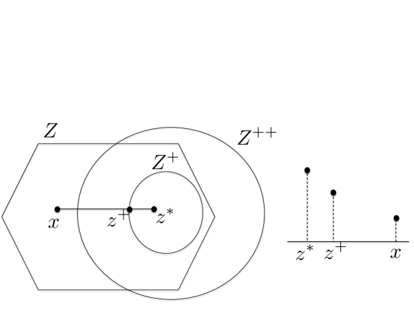
Figure 1: The drawing on the left illustrates the notation used in the proof of Lemma 2. We assume for the sake of a contradiction that there is a points $x\in Z\setminus Z^{++}$. Observe that $Z^{++}$ is a scaled version of $Z^{+}$. The drawing on the right illustrates the contradiction. A function that drops by $\alpha/2$ from $z^{*}$ to $z^{+}$ and by at most $2\varepsilon t$ from $z^{*}$ to $x$ cannot be concave.

Proof  Figure 1 illustrates the definitions used in the proof of Lemma 2. Assume otherwise, i.e., there is $z^{*}\in Z$ with $g_{t}(z^{*})>\frac{\varepsilon^{2}}{3}t+\alpha+\ln(2\Phi(0))$. Let $\lambda^{*}=\alpha/(4\varepsilon t)<1$,

$$Z^{+}=\{z\in Z|g_{t}(z)\geq g_{t}(z^{*})-\alpha/2\},\text{ and }Z^{++}=\{z^{*}+\frac{1}{\lambda^{*}}(z-z^{*})|z\in Z^{+}\}.$$

Concavity of $g_{t}$ implies convexity of $Z^{+}$. Thus, for every $z\in Z^{+}$ and every $\lambda^{\prime}$, $0\leq\lambda^{\prime}\leq 1/\lambda^{*}$, we have $\lambda^{*}\lambda^{\prime}z+(1-\lambda^{*}\lambda^{\prime})z^{*}\in Z^{+}$, and hence

$$z^{*}+\frac{1}{\lambda*}(\lambda^{*}\lambda^{\prime}z+(1-\lambda^{*}\lambda^{\prime})z^{*}-z^{*})=z^{*}+\lambda^{\prime}(z-z^{*})\in Z^{++}.$$

Thus, for every $z\in Z^{+}$, the entire ray $\{z^{*}+\lambda^{\prime}(z-z^{*})|0\leq\lambda^{\prime}\leq 1/\lambda^{*}\}$ belongs to $Z^{++}$. In particular, $Z^{+}\subseteq Z^{++}$.

We next show $Z\subseteq Z^{++}$. Toward a contradiction assume that $x\in Z\setminus Z^{++}$ (and hence $x\in Z\setminus Z^{+}$). Let us define

$$\lambda^{+}=\sup\{\lambda~{}|~{}{z^{*}+\lambda(x-z^{*})\in Z^{+}}\}~{}\text{and }z^{+}=z^{*}+\lambda^{+}(x-z^{*}).$$

By continuity of $g_{t}$, $z^{+}\in Z^{+}$ and $g_{t}(z^{*})-\alpha/2=g_{t}(z^{+})$. By definition of $z^{+}$, we have $x-z^{*}=\frac{1}{{\lambda^{+}}}(z^{+}-z^{*})$ and hence

$$\frac{1}{{\lambda^{+}}}>\frac{1}{\lambda^{*}}.$$ (17)

But $z^{+}=\lambda^{+}x+(1-{\lambda^{+}})z^{*}$ and hence

$$g_{t}(z^{*})-\alpha/2=g_{t}(z^{+})=g_{t}(\lambda^{+}x+(1-{\lambda^{+}})z^{*})\geq\lambda^{+}g_{t}(x)+(1-{\lambda^{+}})g_{t}(z^{*}).$$

Thus

$$\frac{\alpha}{2}\leq\lambda^{+}(g_{t}(z^{*})-g_{t}(x))\leq\lambda^{+}(|g_{t}(z^{*})|+|g_{t}(x)|)\leq 2\varepsilon t\lambda^{+}$$

where the last inequality comes from (13) because $z^{*},x\in Z$. Therefore we have $\lambda^{+}\geq\frac{\alpha}{4\varepsilon t}=\lambda^{*}$ which contradicts (17).

We have now established $Z\subseteq Z^{++}$. By definition, we have $Z^{++}=\frac{1}{\lambda^{*}}Z^{+}+(1-\frac{1}{\lambda^{*}})z^{*}$. Since the volume of a body is invariant under translation, we have

$$\mathop{vol}(Z)\leq\mathop{vol}(Z^{++})=\mathop{vol}\left(\frac{1}{\lambda^{*}}Z^{+}\right)=\left(\frac{1}{\lambda^{*}}\right)^{N}\mathop{vol}(Z^{+})$$

and further

$$\Phi(t) =\int_{z\in Z}e^{g_{t}(z)}dz\geq\int_{z\in Z^{+}}e^{g_{t}(z)}dz$$

$$\geq 2\Phi(0)e^{\frac{\varepsilon^{2}}{3}t+\frac{1}{2}\alpha}\mathop{vol}(Z^{+})\geq 2\Phi(0)e^{\frac{\varepsilon^{2}}{3}t+\frac{1}{2}\alpha}\left(\frac{\alpha}{4\varepsilon t}\right)^{N}\mathop{vol}(Z)>2\Phi(0)e^{\frac{\varepsilon^{2}}{3}t},$$

a contradiction to (11). $\square$

We can now derive an upper-bound on the number of iterations needed to converge to $\varepsilon$-optimal strategies.

Lemma 3

If (16) holds, $\varepsilon\in(0,1)$, $\alpha>0$, and

$$t\geq\frac{6}{\varepsilon^{2}}(\alpha+\max\{0,\ln(2\mathop{vol}(Z))\}),$$ (18)

then $(x(t),y(t))$ is an $\varepsilon$-optimal pair and (14) holds.

Proof  By (16) we have $g_{t}(z)\leq\frac{\varepsilon^{2}}{3}t+\alpha+\ln(2\Phi(0))=\frac{\varepsilon^{2}}{3}t+\alpha+\ln(2\mathop{vol}(Z))$ for all $z\in Z$, or equivalently,

$$\frac{\varepsilon}{2}t(F(x(t),\eta)-F(\xi,y(t)))\leq\frac{\varepsilon^{2}}{3}t+\alpha+\ln(2\mathop{vol}(Z))~{}~{}~{}~{}\text{for all}~{}\xi\in X\text{~{}and~{}}\eta\in Y.$$

Hence,

$$F(x(t),\eta)\leq F(\xi,y(t))+\frac{2\varepsilon}{3}+\frac{2}{\varepsilon t}(\alpha+\ln(2\mathop{vol}(Z))~{}~{}~{}~{}\text{for all}~{}\xi\in X\text{~{}and~{}}\eta\in Y,$$

which implies by (18) that

$$F(x(t),\eta)\leq F(\xi,y(t))+\varepsilon~{}~{}~{}~{}\text{for all}~{}\xi\in X\text{~{}and~{}}\eta\in Y.$$

Finally, (14) holds since $4\varepsilon t\geq 24\alpha/\varepsilon>\alpha$. $\square$

Lemma 4

For any $\varepsilon\in(0,1)$, there exist $\alpha$ and

$$t=O\left(\frac{N}{\varepsilon^{2}}\ln\frac{R}{\varepsilon}\right)$$

satisfying (14), (15) and (18).

Proof  If $\mathop{vol}(Z)\leq\frac{1}{2}$. Let us choose $t=\frac{6\alpha}{\varepsilon^{2}}$. Then $(\ref{e4.2})$ becomes (after taking logarithms)

$$\frac{\alpha}{2}+N\ln\left(\frac{\alpha}{4\varepsilon t}\right)+\ln(\mathop{vol}(Z))>0.$$

So choosing $\frac{\alpha}{2}=N\ln(\frac{25}{\varepsilon})-\ln(\mathop{vol}(Z)))$ would satisfy this inequality. Then

$$t=O\left(\frac{N}{\varepsilon^{2}}\ln\frac{1}{\varepsilon}+\frac{1}{\varepsilon^{2}}\ln\frac{1}{\mathop{vol}(Z)}\right).$$

Since $1/\mathop{vol}{Z}\leq R^{N}$, the claim follows.

If $\mathop{vol}(Z)>\frac{1}{2}$ then

$$e^{\frac{\alpha}{2}}\left(\frac{\alpha}{4\varepsilon t}\right)^{N}\mathop{vol}(Z)>\frac{1}{2}e^{\frac{\alpha}{2}}\left(\frac{\alpha}{4\varepsilon t}\right)^{N},$$

Thus, in order to satisfy (15), it is enough to find $\alpha$ and $t$ satisfying

$$\frac{1}{2}e^{\frac{\alpha}{2}}\left(\frac{\alpha}{4\varepsilon t}\right)^{N}>1.$$

To satisfy (18), let us simply choose $t=\frac{6\alpha}{\varepsilon^{2}}+\frac{6}{\varepsilon^{2}}\ln(2\mathop{vol}(Z))$ and demand that

$$\frac{1}{2}e^{\frac{\alpha}{2}}\left(\frac{\alpha}{4\varepsilon t}\right)^{N}=\frac{1}{2}e^{\frac{\alpha}{2}}\left(\frac{\alpha}{\frac{24\alpha}{\varepsilon}+\frac{24}{\varepsilon}\ln(2\mathop{vol}(Z))}\right)^{N}>1,$$

or equivalently,

$$2\left(\frac{24}{\varepsilon}\right)^{N}\left(1+\frac{\ln(2\mathop{vol}(Z))}{\alpha}\right)^{N}<e^{\frac{\alpha}{2}}.$$

Thus, it is enough to select $\alpha=\max\left\{4(\ln 2+N\ln(\frac{24}{\varepsilon})),2\sqrt{N\ln(2\mathop{vol}(Z))}\right\}$ which satisfies

$$2\left(\frac{24}{\varepsilon}\right)^{N}\leq e^{\frac{\alpha}{4}}~{}\text{ and }~{}\left(1+\frac{\ln(2\mathop{vol}(Z))}{\alpha}\right)^{N}<e^{\frac{\ln(2\mathop{vol}(Z))}{\alpha}N}\leq e^{\frac{\alpha}{4}}.$$

It follows that

$$t=\max\left\{\frac{24}{\varepsilon^{2}}(\ln 2+N\ln(\frac{24}{\varepsilon})),\frac{12}{\varepsilon^{2}}\sqrt{N\ln(2\mathop{vol}(Z))}\right\}+\frac{6}{\varepsilon^{2}}\ln(2\mathop{vol}(Z)).$$

Since $\mathop{vol}(Z)\leq R^{N}$, the claim follows.

In both cases (14) holds by the preceding lemma. $\square$

Corollary 2

Assume $X$ and $Y$ satisfy assumptions (A1) and (A2). Then Algorithm 1, when run with $T$ satisfying the bound in Lemma 4, computes a pair of $\varepsilon$-optimal strategies in expected $O(\frac{n+m}{\varepsilon^{2}}\ln\frac{R}{\varepsilon})$ iterations.

6.3 Using approximate distributions

We now consider the (realistic) situation when we can only sample approximately from the convex sets. In this case we assume the existence of approximate sampling routines that, upon the call in step 3 of the algorithm, return vectors $\xi\in X$, and (independently) $\eta\in Y$, with densities $\hat{p}_{\xi}(t)$ and $\hat{q}_{\eta}(t)$, such that

$$\sup_{X^{\prime}\subseteq X}\left|\frac{\hat{p}_{X^{\prime}}(t)}{\hat{p}_{X}(t)}-\frac{p_{X^{\prime}}(t)}{p_{X}(t)}\right|\leq\delta~{}~{}\mbox{ and }~{}~{}\sup_{Y^{\prime}\subseteq Y}\left|\frac{\hat{q}_{Y^{\prime}}(t)}{\hat{q}_{Y}(t)}-\frac{q_{Y^{\prime}}(t)}{q_{Y}(t)}\right|\leq\delta,$$ (19)

where $\hat{p}_{X^{\prime}}(t)=\int_{\xi\in X^{\prime}}\hat{p}_{\xi}d\xi$ (similarly, define $p_{X^{\prime}}(t),\hat{q}_{Y^{\prime}}(t),q_{Y^{\prime}}(t)$), and $\delta$ is a given desired accuracy. We next prove an approximate version of Lemma 1.

Lemma 5

Suppose that we use approximate sampling routines with $\delta=\varepsilon/4$ in step 3 of Algorithm 1. Then, for $t=0,1,2,\ldots,$ we have

$$\mathbb{E}[\Phi(t+1)]\leq\mathbb{E}[\Phi(t)](1+\frac{43}{36}\varepsilon^{2}).$$

Proof  The argument up to Equation (6.1) remains the same. Taking the expectation with respect to $\eta$ (with density proportional to $\hat{q}_{\eta}(t)$), we get

$$\mathbb{E}_{\hat{q}}[\|p(t+1)\|_{1}]\leq\|p(t)\|_{1}\left[1+\frac{\varepsilon^{2}}{6}-\frac{\varepsilon}{2}\frac{\int_{\eta\in Y}\hat{q}_{\eta}(t)\int_{\xi\in X}p_{\xi}(t)F(\xi,\eta)d\xi d\eta}{\|\hat{q}(t)\|_{1}\|p(t)\|_{1}}\right].$$ (20)

Similarly,

$$\mathbb{E}_{\hat{p}}[\|q(t+1)\|_{1}]\leq\|q(t)\|_{1}\left[1+\frac{\varepsilon^{2}}{6}+\frac{\varepsilon}{2}\frac{\int_{\xi\in X}\hat{p}_{\xi}(t)\int_{\eta\in Y}q_{\eta}(t)F(\xi,\eta)d\eta d\xi}{\|\hat{p}(t)\|_{1}\|q(t)\|_{1}}\right].$$ (21)

Thus, by independence of $\xi$ and $\eta$, we have

$$\mathbb{E}[\Phi(t+1)|x(t),y(t)] \leq \Phi(t)\left[\left(1+\frac{\varepsilon^{2}}{6}\right)^{2}\right.$$

$$+\left.\frac{\varepsilon}{2}\left(1+\frac{\varepsilon^{2}}{6}\right)\left(\frac{\int_{\xi\in X}\hat{p}_{\xi}(t)\int_{\eta\in Y}q_{\eta}(t)F(\xi,\eta)d\eta d\xi}{|\hat{p}(t)|\|q(t)\|_{1}}-\frac{\int_{\eta\in Y}\hat{q}_{\eta}(t)\int_{\xi\in X}p_{\xi}(t)F(\xi,\eta)d\xi d\eta}{\|\hat{q}(t)\|_{1}\|p(t)\|_{1}}\right)\right.$$

$$-\left.\frac{\varepsilon^{2}}{4}\frac{\int_{\xi\in X}\hat{p}_{\xi}(t)\int_{\eta\in Y}q_{\eta}(t)F(\xi,\eta)d\eta d\xi}{\|\hat{p}(t)\|_{1}\|q(t)\|_{1}}.\frac{\int_{\eta\in Y}\hat{q}_{\eta}(t)\int_{\xi\in X}p_{\xi}(t)F(\xi,\eta)d\xi d\eta}{\|\hat{q}(t)\|_{1}\|p(t)\|_{1}}\right].$$

We will make use of the following proposition.

Proposition 1

If we set $\delta=\varepsilon/4$ in (19), then

$$\left|\frac{\int_{\xi\in X}\hat{p}_{\xi}(t)\int_{\eta\in Y}q_{\eta}(t)F(\xi,\eta)d\eta d\xi}{|\hat{p}(t)|\|q(t)\|_{1}}-\frac{\int_{\eta\in Y}\hat{q}_{\eta}(t)\int_{\xi\in X}p_{\xi}(t)F(\xi,\eta)d\xi d\eta}{|\hat{q}(t)\|_{1}\|p(t)\|_{1}}\right|\leq\varepsilon.$$ (22)

Proof  Since

$$\frac{\int_{\xi\in X}p_{\xi}(t)\int_{\eta\in Y}q_{\eta}(t)F(\xi,\eta)d\eta d\xi}{\|p(t)\|_{1}\|q(t)\|_{1}}=\frac{\int_{\eta\in Y}q_{\eta}(t)\int_{\xi\in X}p_{\xi}(t)F(\xi,\eta)d\xi d\eta}{\|q(t)\|_{1}\|p(t)\|_{1}},$$

we can bound the L.H.S. of (22) by

$$\left|\frac{\int_{\xi\in X}p_{\xi}(t)\int_{\eta\in Y}q_{\eta}(t)F(\xi,\eta)d\eta d\xi}{\|p(t)\|_{1}\|q(t)\|_{1}}-\frac{\int_{\xi\in X}\hat{p}_{\xi}(t)\int_{\eta\in Y}q_{\eta}(t)F(\xi,\eta)d\eta d\xi}{|\hat{p}(t)|\|q(t)\|_{1}}\right|+$$

$$\left|\frac{\int_{\eta\in Y}q_{\eta}(t)\int_{\xi\in X}p_{\xi}(t)F(\xi,\eta)d\xi d\eta}{\|q(t)\|_{1}\|p(t)\|_{1}}-\frac{\int_{\eta\in Y}\hat{q}_{\eta}(t)\int_{\xi\in X}p_{\xi}(t)F(\xi,\eta)d\xi d\eta}{\|\hat{q}(t)\|_{1}\|p(t)\|_{1}}\right|.$$ (23)

Thus it is enough to show that each term in (23) is at most $\frac{\varepsilon}{2}$. Since the two terms are similar, we only consider the first term. Define $X^{\prime}=\{\xi\in X~{}:~{}\frac{p_{\xi}(t)}{p_{X}(t)}\geq\frac{\hat{p}_{\xi}(t)}{\hat{p}_{X}(t)}\}$ and $X^{\prime\prime}=X\setminus X^{\prime}$.

$$~{}\frac{1}{\|q(t)\|_{1}}\left|\int_{\xi\in X}\int_{\eta\in Y}q_{\eta}(t)F(\xi,\eta)\left(\frac{p_{\xi}(t)}{\|p(t)\|_{1}}-\frac{\hat{p}_{\xi}(t)}{|\hat{p}(t)|}\right)d\eta d\xi\right|$$

$$~{}~{}~{}~{}~{}~{}~{}~{}~{}~{}~{}~{}~{}~{}~{}~{}~{}~{}~{}~{}~{}~{}~{}\leq\frac{1}{q_{Y}(t)}\int_{\xi\in X}\int_{\eta\in Y}q_{\eta}(t)|F(\xi,\eta)|\left|\frac{p_{\xi}(t)}{p_{X}(t)}-\frac{\hat{p}_{\xi}(t)}{\hat{p}_{X}(t)}\right|d\eta d\xi$$

$$~{}~{}~{}~{}~{}~{}~{}~{}~{}~{}~{}~{}~{}~{}~{}~{}~{}~{}~{}~{}~{}~{}~{}\leq\frac{1}{q_{Y}(t)}\int_{\xi\in X}\int_{\eta\in Y}q_{\eta}(t)\left|\frac{p_{\xi}(t)}{p_{X}(t)}-\frac{\hat{p}_{\xi}(t)}{\hat{p}_{X}(t)}\right|d\eta d\xi~{}\mbox{ (by (A2))~{}}$$

$$~{}~{}~{}~{}~{}~{}~{}~{}~{}~{}~{}~{}~{}~{}~{}~{}~{}~{}~{}~{}~{}~{}~{}=\int_{\xi\in X}\left|\frac{p_{\xi}(t)}{p_{X}(t)}-\frac{\hat{p}_{\xi}(t)}{\hat{p}_{X}(t)}\right|d\xi$$

$$~{}~{}~{}~{}~{}~{}~{}~{}~{}~{}~{}~{}~{}~{}~{}~{}~{}~{}~{}~{}~{}~{}~{}=\int_{\xi\in X^{\prime}}\left(\frac{p_{\xi}(t)}{p_{X}(t)}-\frac{\hat{p}_{\xi}(t)}{\hat{p}_{X}(t)}\right)d\xi+\int_{\xi\in X^{\prime\prime}}\left(\frac{\hat{p}_{\xi}(t)}{\hat{p}_{X}(t)}-\frac{p_{\xi}(t)}{p_{X}(t)}\right)d\xi$$

$$~{}~{}~{}~{}~{}~{}~{}~{}~{}~{}~{}~{}~{}~{}~{}~{}~{}~{}~{}~{}~{}~{}~{}=\left(\frac{p_{X^{\prime}}(t)}{p_{X}(t)}-\frac{\hat{p}_{X^{\prime}}(t)}{\hat{p}_{X}(t)}\right)+\left(\frac{\hat{p}_{X^{\prime\prime}}(t)}{\hat{p}_{X}(t)}-\frac{p_{X^{\prime\prime}}(t)}{p_{X}(t)}\right)\leq\frac{\varepsilon}{2}\mbox{ (by(\ref{as}))}.$$

$\square$

Proposition 1 implies that

$$\mathbb{E}[\Phi(t+1)|x(t),y(t)]\leq\Phi(t)\left[\left(1+\frac{\varepsilon^{2}}{6}\right)^{2}+\frac{\varepsilon^{2}}{2}\left(1+\frac{\varepsilon^{2}}{6}\right)+\frac{\varepsilon^{4}}{4}\right]\leq\Phi(t)\left(1+\frac{43}{36}\varepsilon^{2}\right).$$

The rest of the proof is as in Lemma 1. $\square$

Combining the currently known bound on the mixing time for sampling (see [LV06b, LV06a, LV07] and also Section 4) with the bounds on the number of iterations from Corollary 2 gives Theorem 1.

7 Conclusion

We showed that randomized fictitious play can be applied for computing $\varepsilon$-saddle points of convex-concave functions over the product of two convex bounded sets. Even though our bounds were stated for general convex sets, one should note that these bounds may be improved for classes of convex sets for which faster sampling procedures could be developed. We believe that the method used in this paper could be useful for developing algorithms for computing approximate equilibria for other classes of games.

References

• [AHK05] S. Arora, E. Hazan, and S. Kale. Fast algorithms for approximate semidefinite programming using the multiplicative weights update method. In Proc. 46th Symp. Foundations of Computer Science (FOCS), pages 339–348, 2005.
• [AHK12] Sanjeev Arora, Elad Hazan, and Satyen Kale. The multiplicative weights update method: a meta-algorithm and applications. Theory of Computing, 8(1):121–164, 2012.
• [AK07] S. Arora and S. Kale. A combinatorial, primal-dual approach to semidefinite programs. In Proc. 39th Symp. Theory of Computing (STOC), pages 227–236, 2007.
• [BBR04] Y. Bartal, J.W. Byers, and D. Raz. Fast, distributed approximation algorithms for positive linear programming with applications to flow control. SIAM Journal on Computing, 33(6):1261–1279, 2004.
• [Bel97] A. S. Belenky. A 2-person game on a polyhedral set of connected strategies. Computers & Mathematics with Applications, 33(6):99–125, 1997.
• [Bro51] G.W. Brown. Iterative solution of games by fictitious play. In: T.C. Koopmans, Editor, Activity Analysis of Production and Allocation, pages 374 –376, 1951.
• [BV04] D. Bertsimas and S. Vempala. Solving convex programs by random walks. J. ACM, 51(4):540–556, 2004.
• [Dan63] G.B. Dantzig. Linear Programming and Extensions. Princeton University Press, 1963.
• [DJ07] F. Diedrich and K. Jansen. Faster and simpler approximation algorithms for mixed packing and covering problems. Theoretical Computer Science, 377(1-3):182–204, 2007.
• [DKR91] A. Darte, L. Khachiyan, and Y. Robert. Linear scheduling is nearly optimal. Parallel Processing Letters, 1(2):73–81, 1991.
• [FS99] Y. Freund and R.E. Schapire. Adaptive game playing using multiplicative weights. Games and Economic Behavior, 29(1-2):79–103, 1999.
• [GK92] M.D. Grigoriadis and L.G. Khachiyan. Approximate solution of matrix games in parallel. In Advances in Optimization and Parallel Computing, pages 129–136, 1992.
• [GK95] M.D. Grigoriadis and L.G. Khachiyan. A sublinear-time randomized approximation algorithm for matrix games. Operations Research Letters, 18(2):53–58, 1995.
• [GK96] M.D. Grigoriadis and L.G. Khachiyan. Coordination complexity of parallel price-directive decomposition. Mathematics of Operations Research, 21(2):321–340, 1996.
• [GK98] N. Garg and J. Könemann. Faster and simpler algorithms for multicommodity flow and other fractional packing problems. In Proc. 39th Symp. Foundations of Computer Science (FOCS), pages 300–309, 1998.
• [GK04] N. Garg and R. Khandekar. Fractional covering with upper bounds on the variables: Solving lps with negative entries. In Proc. 14th European Symposium on Algorithms (ESA), pages 371–382, 2004.
• [GKPV01] M.D. Grigoriadis, L.G. Khachiyan, L. Porkolab, and J. Villavicencio. Approximate max-min resource sharing for structured concave optimization. SIAM Journal on Optimization, 41:1081–1091, 2001.
• [GLS93] M. Grötschel, L. Lovász, and A. Schrijver. Geometric Algorithms and Combinatorial Optimization, volume 2 of Algorithms and Combinatorics. Springer, second corrected edition, 1993.
• [Gro67] H. Groemer. On the min-max theorem for finite two-person zero-sum games. Probability Theory and Related Fields, 9(1):59–61, 1967.
• [Haz06] E. Hazan. Efficient Algorithms for Online Convex Optimization and Their Application. PhD thesis, Princeton University, USA, 2006.
• [HS06] J. Hofbauer and S. Sorin. Best response dynamics for continuous zero-sum games. Discrete and Continuos Dynamical Systems – Series B, 6(1):215 –224, 2006.
• [Kal07] S. Kale. Efficient Algorithms using the Multiplicative Weights Update Method. PhD thesis, Princeton University, USA, 2007.
• [Kha04] R. Khandekar. Lagrangian Relaxation based Algorithms for Convex Programming Problems. PhD thesis, Indian Institute of Technology, Delhi, 2004.
• [KMN09] T. Kavitha, J. Mestre, and M. Nasre. Popular mixed matchings. In Proc. 36th Intl. Coll. Automata, Languages and Programming (ICALP), pages 574–584, 2009.
• [KV06] A. Kalai and S. Vempala. Simulated annealing for convex optimization. Mathematics of Operations Research, 31(2):253–266, 2006.
• [KY07] C. Koufogiannakis and N.E. Young. Beating simplex for fractional packing and covering linear programs. In Proc. 48th Symp. Foundations of Computer Science (FOCS), pages 494–504, 2007.
• [LN93] M. Luby and N. Nisan. A parallel approximation algorithm for positive linear programming. In Proc. 25th Symp. Theory of Computing (STOC), pages 448–457, 1993.
• [LV06a] L. Lovász and S. Vempala. Fast algorithms for logconcave functions: Sampling, rounding, integration and optimization. In Proc. 47th Symp. Foundations of Computer Science (FOCS), pages 57–68, 2006.
• [LV06b] L. Lovász and Santosh Vempala. Hit-and-run from a corner. SIAM Journal on Computing, 35(4):985–1005, 2006.
• [LV07] L. Lovász and S. Vempala. The geometry of logconcave functions and sampling algorithms. Random Structures and Algorithms, 30(3):307–358, 2007.
• [LW94] N. Littlestone and M.K. Warmuth. The weighted majority algorithm. Information and Computation, 108(2):212–261, 1994.
• [McL84] L. McLinden. A minimax theorem. Mathematics of Operations Research, 9(4):576–591, 1984.
• [PST91] S.A. Plotkin, D.B. Shmoys, and É. Tardos. Fast approximation algorithms for fractional packing and covering problems. In Proc. 32nd Symp. Foundations of Computer Science (FOCS), pages 495–504, 1991.
• [Rob51] J. Robinson. An iterative method of solving a game. Annals of Mathematics, 54(2):296–301, 1951.
• [Roc70] R.T. Rockafellar. Convex Analysis (Princeton Mathematical Series). Princeton University Press, 1970.
• [Sch86] A. Schrijver. Theory of Linear and Integer Programming. Wiley, New York, 1986.
• [Seb90] Z. Sebestyén. A general saddle point theorem and its applications. Acta Mathematica Hungarica, 56(3-4):303–307, 1990.
• [Sha58] H.N. Shapiro. Note on a computation method in the theory of games. Communications on Pure and Applied Mathematics, 11(4):587–593, 1958.
• [Ter72] F. Terkelsen. Some minimax theorems. Mathematica Scandinavica, 31:405–413, 1972.
• [tKP90] In-sook Kim and S. Park. Saddle point theorems on generalized convex spaces. Journal of Inequalities and Applications, 5(4):397–405, 1990.
• [Vem05] S. Vempala. Geometric random walks: A survey. Combinatorial and Computational Geometry, MSRI Publications, 52:573–612, 2005.
• [Vor84] N. Vorob’ev. Foundations of Game Theory: Noncooperative Games, volume 2. Birkhäuser, 1984.
• [Wal45] A. Wald. Generalization of a theorem by v. Neumann concerning zero-sum two person games. Annals of Mathematics, 46(2):281–286, 1945.
• [Was03] A.R. Washburn. Two-Person Zero-Sum Games. INFORMS, 2003.
• [You01] N.E. Young. Sequential and parallel algorithms for mixed packing and covering. In Proc. 42nd Symp. Foundations of Computer Science (FOCS), pages 538–546, 2001.