EUROPEAN ORGANIZATION FOR NUCLEAR RESEARCH (CERN)

​​​ CERN-PH-EP-2013-004 LHCb-PAPER-2012-045 January 24, 2013

Analysis of the resonant components in $\kern 3.73305pt\overline{\kern-3.73305ptB}{}^{0}\rightarrow{J\mskip-3.0mu/\mskip-2.0mu\psi\mskip 2.0mu}\pi^{+}\pi^{-}$

The LHCb collaboration

Interpretation of $C\!P$ violation measurements using charmonium decays, in both the $\kern 1.79993pt\overline{\kern-1.79993ptB}{}^{0}$ and $\kern 1.79993pt\overline{\kern-1.79993ptB}{}^{0}_{s}$ systems, can be subject to changes due to “penguin” type diagrams. These effects can be investigated using measurements of the Cabibbo-suppressed $\kern 1.79993pt\overline{\kern-1.79993ptB}{}^{0}\rightarrow{J\mskip-3.0mu/\mskip-2.0mu\psi\mskip 2.0mu}\pi^{+}\pi^{-}$ decays. The final state composition of this channel is investigated using a 1.0 fb^-1 sample of data produced in 7 TeV $pp$ collisions at the LHC and collected by the LHCb experiment. A modified Dalitz plot analysis is performed using both the invariant mass spectra and the decay angular distributions. An improved measurement of the $\kern 1.79993pt\overline{\kern-1.79993ptB}{}^{0}\rightarrow{J\mskip-3.0mu/\mskip-2.0mu\psi\mskip 2.0mu}\pi^{+}\pi^{-}$ branching fraction of $(3.97\pm 0.09\pm 0.11\pm 0.16)\times 10^{-5}$ is reported where the first uncertainty is statistical, the second is systematic and the third is due to the uncertainty of the branching fraction of the decay $B^{-}\rightarrow{J\mskip-3.0mu/\mskip-2.0mu\psi\mskip 2.0mu}K^{-}$ used as a normalization channel. Significant production of $f_{0}(500)$ and $\rho(770)$ resonances is found in the substructure of the ${J\mskip-3.0mu/\mskip-2.0mu\psi\mskip 2.0mu}\pi^{+}\pi^{-}$ final state, and this indicates that they are viable final states for $C\!P$ violation studies. In contrast evidence for the $f_{0}(980)$ resonance is not found. This allows us to establish the first upper limit on the branching fraction product ${\cal{B}}\left(\kern 1.79993pt\overline{\kern-1.79993ptB}{}^{0}\rightarrow{J\mskip-3.0mu/\mskip-2.0mu\psi\mskip 2.0mu}f_{0}(980)\right)\times{\cal{B}}\left(f_{0}(980)\rightarrow\pi^{+}\pi^{-}\right)<1.1\times 10^{-6}$, leading to an upper limit on the absolute value of the mixing angle of the $f_{0}(980)$ with the $f_{0}(500)$ of less than $31^{\circ}$, both at 90% confidence level.

Submitted to Physical Review D

© CERN on behalf of the LHCb collaboration, license CC-BY-3.0.

LHCb collaboration

R. Aaij³⁸, C. Abellan Beteta^33,n, A. Adametz¹¹, B. Adeva³⁴, M. Adinolfi⁴³, C. Adrover⁶, A. Affolder⁴⁹, Z. Ajaltouni⁵, J. Albrecht⁹, F. Alessio³⁵, M. Alexander⁴⁸, S. Ali³⁸, G. Alkhazov²⁷, P. Alvarez Cartelle³⁴, A.A. Alves Jr^22,35, S. Amato², Y. Amhis⁷, L. Anderlini^17,f, J. Anderson³⁷, R. Andreassen⁵⁷, R.B. Appleby⁵¹, O. Aquines Gutierrez¹⁰, F. Archilli¹⁸, A. Artamonov ³², M. Artuso⁵³, E. Aslanides⁶, G. Auriemma^22,m, S. Bachmann¹¹, J.J. Back⁴⁵, C. Baesso⁵⁴, V. Balagura²⁸, W. Baldini¹⁶, R.J. Barlow⁵¹, C. Barschel³⁵, S. Barsuk⁷, W. Barter⁴⁴, Th. Bauer³⁸, A. Bay³⁶, J. Beddow⁴⁸, I. Bediaga¹, S. Belogurov²⁸, K. Belous³², I. Belyaev²⁸, E. Ben-Haim⁸, M. Benayoun⁸, G. Bencivenni¹⁸, S. Benson⁴⁷, J. Benton⁴³, A. Berezhnoy²⁹, R. Bernet³⁷, M.-O. Bettler⁴⁴, M. van Beuzekom³⁸, A. Bien¹¹, S. Bifani¹², T. Bird⁵¹, A. Bizzeti^17,h, P.M. Bjørnstad⁵¹, T. Blake³⁵, F. Blanc³⁶, C. Blanks⁵⁰, J. Blouw¹¹, S. Blusk⁵³, A. Bobrov³¹, V. Bocci²², A. Bondar³¹, N. Bondar²⁷, W. Bonivento¹⁵, S. Borghi⁵¹, A. Borgia⁵³, T.J.V. Bowcock⁴⁹, E. Bowen³⁷, C. Bozzi¹⁶, T. Brambach⁹, J. van den Brand³⁹, J. Bressieux³⁶, D. Brett⁵¹, M. Britsch¹⁰, T. Britton⁵³, N.H. Brook⁴³, H. Brown⁴⁹, I. Burducea²⁶, A. Bursche³⁷, J. Buytaert³⁵, S. Cadeddu¹⁵, O. Callot⁷, M. Calvi^20,j, M. Calvo Gomez^33,n, A. Camboni³³, P. Campana^18,35, A. Carbone^14,c, G. Carboni^21,k, R. Cardinale^19,i, A. Cardini¹⁵, H. Carranza-Mejia⁴⁷, L. Carson⁵⁰, K. Carvalho Akiba², G. Casse⁴⁹, M. Cattaneo³⁵, Ch. Cauet⁹, M. Charles⁵², Ph. Charpentier³⁵, P. Chen^3,36, N. Chiapolini³⁷, M. Chrzaszcz ²³, K. Ciba³⁵, X. Cid Vidal³⁴, G. Ciezarek⁵⁰, P.E.L. Clarke⁴⁷, M. Clemencic³⁵, H.V. Cliff⁴⁴, J. Closier³⁵, C. Coca²⁶, V. Coco³⁸, J. Cogan⁶, E. Cogneras⁵, P. Collins³⁵, A. Comerma-Montells³³, A. Contu¹⁵, A. Cook⁴³, M. Coombes⁴³, G. Corti³⁵, B. Couturier³⁵, G.A. Cowan³⁶, D. Craik⁴⁵, S. Cunliffe⁵⁰, R. Currie⁴⁷, C. D’Ambrosio³⁵, P. David⁸, P.N.Y. David³⁸, I. De Bonis⁴, K. De Bruyn³⁸, S. De Capua⁵¹, M. De Cian³⁷, J.M. De Miranda¹, L. De Paula², W. De Silva⁵⁷, P. De Simone¹⁸, D. Decamp⁴, M. Deckenhoff⁹, H. Degaudenzi^36,35, L. Del Buono⁸, C. Deplano¹⁵, D. Derkach¹⁴, O. Deschamps⁵, F. Dettori³⁹, A. Di Canto¹¹, J. Dickens⁴⁴, H. Dijkstra³⁵, P. Diniz Batista¹, M. Dogaru²⁶, F. Domingo Bonal^33,n, S. Donleavy⁴⁹, F. Dordei¹¹, A. Dosil Suárez³⁴, D. Dossett⁴⁵, A. Dovbnya⁴⁰, F. Dupertuis³⁶, R. Dzhelyadin³², A. Dziurda²³, A. Dzyuba²⁷, S. Easo^46,35, U. Egede⁵⁰, V. Egorychev²⁸, S. Eidelman³¹, D. van Eijk³⁸, S. Eisenhardt⁴⁷, U. Eitschberger⁹, R. Ekelhof⁹, L. Eklund⁴⁸, I. El Rifai⁵, Ch. Elsasser³⁷, D. Elsby⁴², A. Falabella^14,e, C. Färber¹¹, G. Fardell⁴⁷, C. Farinelli³⁸, S. Farry¹², V. Fave³⁶, D. Ferguson⁴⁷, V. Fernandez Albor³⁴, F. Ferreira Rodrigues¹, M. Ferro-Luzzi³⁵, S. Filippov³⁰, C. Fitzpatrick³⁵, M. Fontana¹⁰, F. Fontanelli^19,i, R. Forty³⁵, O. Francisco², M. Frank³⁵, C. Frei³⁵, M. Frosini^17,f, S. Furcas²⁰, E. Furfaro²¹, A. Gallas Torreira³⁴, D. Galli^14,c, M. Gandelman², P. Gandini⁵², Y. Gao³, J. Garofoli⁵³, P. Garosi⁵¹, J. Garra Tico⁴⁴, L. Garrido³³, C. Gaspar³⁵, R. Gauld⁵², E. Gersabeck¹¹, M. Gersabeck⁵¹, T. Gershon^45,35, Ph. Ghez⁴, V. Gibson⁴⁴, V.V. Gligorov³⁵, C. Göbel⁵⁴, D. Golubkov²⁸, A. Golutvin^50,28,35, A. Gomes², H. Gordon⁵², M. Grabalosa Gándara⁵, R. Graciani Diaz³³, L.A. Granado Cardoso³⁵, E. Graugés³³, G. Graziani¹⁷, A. Grecu²⁶, E. Greening⁵², S. Gregson⁴⁴, O. Grünberg⁵⁵, B. Gui⁵³, E. Gushchin³⁰, Yu. Guz³², T. Gys³⁵, C. Hadjivasiliou⁵³, G. Haefeli³⁶, C. Haen³⁵, S.C. Haines⁴⁴, S. Hall⁵⁰, T. Hampson⁴³, S. Hansmann-Menzemer¹¹, N. Harnew⁵², S.T. Harnew⁴³, J. Harrison⁵¹, P.F. Harrison⁴⁵, T. Hartmann⁵⁵, J. He⁷, V. Heijne³⁸, K. Hennessy⁴⁹, P. Henrard⁵, J.A. Hernando Morata³⁴, E. van Herwijnen³⁵, E. Hicks⁴⁹, D. Hill⁵², M. Hoballah⁵, C. Hombach⁵¹, P. Hopchev⁴, W. Hulsbergen³⁸, P. Hunt⁵², T. Huse⁴⁹, N. Hussain⁵², D. Hutchcroft⁴⁹, D. Hynds⁴⁸, V. Iakovenko⁴¹, P. Ilten¹², R. Jacobsson³⁵, A. Jaeger¹¹, E. Jans³⁸, F. Jansen³⁸, P. Jaton³⁶, F. Jing³, M. John⁵², D. Johnson⁵², C.R. Jones⁴⁴, B. Jost³⁵, M. Kaballo⁹, S. Kandybei⁴⁰, M. Karacson³⁵, T.M. Karbach³⁵, I.R. Kenyon⁴², U. Kerzel³⁵, T. Ketel³⁹, A. Keune³⁶, B. Khanji²⁰, O. Kochebina⁷, I. Komarov^36,29, R.F. Koopman³⁹, P. Koppenburg³⁸, M. Korolev²⁹, A. Kozlinskiy³⁸, L. Kravchuk³⁰, K. Kreplin¹¹, M. Kreps⁴⁵, G. Krocker¹¹, P. Krokovny³¹, F. Kruse⁹, M. Kucharczyk^20,23,j, V. Kudryavtsev³¹, T. Kvaratskheliya^28,35, V.N. La Thi³⁶, D. Lacarrere³⁵, G. Lafferty⁵¹, A. Lai¹⁵, D. Lambert⁴⁷, R.W. Lambert³⁹, E. Lanciotti³⁵, G. Lanfranchi^18,35, C. Langenbruch³⁵, T. Latham⁴⁵, C. Lazzeroni⁴², R. Le Gac⁶, J. van Leerdam³⁸, J.-P. Lees⁴, R. Lefèvre⁵, A. Leflat^29,35, J. Lefrançois⁷, O. Leroy⁶, Y. Li³, L. Li Gioi⁵, M. Liles⁴⁹, R. Lindner³⁵, C. Linn¹¹, B. Liu³, G. Liu³⁵, J. von Loeben²⁰, J.H. Lopes², E. Lopez Asamar³³, N. Lopez-March³⁶, H. Lu³, J. Luisier³⁶, H. Luo⁴⁷, F. Machefert⁷, I.V. Machikhiliyan^4,28, F. Maciuc²⁶, O. Maev^27,35, S. Malde⁵², G. Manca^15,d, G. Mancinelli⁶, N. Mangiafave⁴⁴, U. Marconi¹⁴, R. Märki³⁶, J. Marks¹¹, G. Martellotti²², A. Martens⁸, L. Martin⁵², A. Martín Sánchez⁷, M. Martinelli³⁸, D. Martinez Santos³⁹, D. Martins Tostes², A. Massafferri¹, R. Matev³⁵, Z. Mathe³⁵, C. Matteuzzi²⁰, M. Matveev²⁷, E. Maurice⁶, A. Mazurov^16,30,35,e, J. McCarthy⁴², R. McNulty¹², B. Meadows^57,52, F. Meier⁹, M. Meissner¹¹, M. Merk³⁸, D.A. Milanes⁸, M.-N. Minard⁴, J. Molina Rodriguez⁵⁴, S. Monteil⁵, D. Moran⁵¹, P. Morawski²³, R. Mountain⁵³, I. Mous³⁸, F. Muheim⁴⁷, K. Müller³⁷, R. Muresan²⁶, B. Muryn²⁴, B. Muster³⁶, P. Naik⁴³, T. Nakada³⁶, R. Nandakumar⁴⁶, I. Nasteva¹, M. Needham⁴⁷, N. Neufeld³⁵, A.D. Nguyen³⁶, T.D. Nguyen³⁶, C. Nguyen-Mau^36,o, M. Nicol⁷, V. Niess⁵, R. Niet⁹, N. Nikitin²⁹, T. Nikodem¹¹, S. Nisar⁵⁶, A. Nomerotski⁵², A. Novoselov³², A. Oblakowska-Mucha²⁴, V. Obraztsov³², S. Oggero³⁸, S. Ogilvy⁴⁸, O. Okhrimenko⁴¹, R. Oldeman^15,d,35, M. Orlandea²⁶, J.M. Otalora Goicochea², P. Owen⁵⁰, B.K. Pal⁵³, A. Palano^13,b, M. Palutan¹⁸, J. Panman³⁵, A. Papanestis⁴⁶, M. Pappagallo⁴⁸, C. Parkes⁵¹, C.J. Parkinson⁵⁰, G. Passaleva¹⁷, G.D. Patel⁴⁹, M. Patel⁵⁰, G.N. Patrick⁴⁶, C. Patrignani^19,i, C. Pavel-Nicorescu²⁶, A. Pazos Alvarez³⁴, A. Pellegrino³⁸, G. Penso^22,l, M. Pepe Altarelli³⁵, S. Perazzini^14,c, D.L. Perego^20,j, E. Perez Trigo³⁴, A. Pérez-Calero Yzquierdo³³, P. Perret⁵, M. Perrin-Terrin⁶, G. Pessina²⁰, K. Petridis⁵⁰, A. Petrolini^19,i, A. Phan⁵³, E. Picatoste Olloqui³³, B. Pietrzyk⁴, T. Pilař⁴⁵, D. Pinci²², S. Playfer⁴⁷, M. Plo Casasus³⁴, F. Polci⁸, G. Polok²³, A. Poluektov^45,31, E. Polycarpo², D. Popov¹⁰, B. Popovici²⁶, C. Potterat³³, A. Powell⁵², J. Prisciandaro³⁶, V. Pugatch⁴¹, A. Puig Navarro³⁶, W. Qian⁴, J.H. Rademacker⁴³, B. Rakotomiaramanana³⁶, M.S. Rangel², I. Raniuk⁴⁰, N. Rauschmayr³⁵, G. Raven³⁹, S. Redford⁵², M.M. Reid⁴⁵, A.C. dos Reis¹, S. Ricciardi⁴⁶, A. Richards⁵⁰, K. Rinnert⁴⁹, V. Rives Molina³³, D.A. Roa Romero⁵, P. Robbe⁷, E. Rodrigues⁵¹, P. Rodriguez Perez³⁴, G.J. Rogers⁴⁴, S. Roiser³⁵, V. Romanovsky³², A. Romero Vidal³⁴, J. Rouvinet³⁶, T. Ruf³⁵, H. Ruiz³³, G. Sabatino^22,k, J.J. Saborido Silva³⁴, N. Sagidova²⁷, P. Sail⁴⁸, B. Saitta^15,d, C. Salzmann³⁷, B. Sanmartin Sedes³⁴, M. Sannino^19,i, R. Santacesaria²², C. Santamarina Rios³⁴, E. Santovetti^21,k, M. Sapunov⁶, A. Sarti^18,l, C. Satriano^22,m, A. Satta²¹, M. Savrie^16,e, D. Savrina^28,29, P. Schaack⁵⁰, M. Schiller³⁹, H. Schindler³⁵, S. Schleich⁹, M. Schlupp⁹, M. Schmelling¹⁰, B. Schmidt³⁵, O. Schneider³⁶, A. Schopper³⁵, M.-H. Schune⁷, R. Schwemmer³⁵, B. Sciascia¹⁸, A. Sciubba^18,l, M. Seco³⁴, A. Semennikov²⁸, K. Senderowska²⁴, I. Sepp⁵⁰, N. Serra³⁷, J. Serrano⁶, P. Seyfert¹¹, M. Shapkin³², I. Shapoval^40,35, P. Shatalov²⁸, Y. Shcheglov²⁷, T. Shears^49,35, L. Shekhtman³¹, O. Shevchenko⁴⁰, V. Shevchenko²⁸, A. Shires⁵⁰, R. Silva Coutinho⁴⁵, T. Skwarnicki⁵³, N.A. Smith⁴⁹, E. Smith^52,46, M. Smith⁵¹, K. Sobczak⁵, M.D. Sokoloff⁵⁷, F.J.P. Soler⁴⁸, F. Soomro^18,35, D. Souza⁴³, B. Souza De Paula², B. Spaan⁹, A. Sparkes⁴⁷, P. Spradlin⁴⁸, F. Stagni³⁵, S. Stahl¹¹, O. Steinkamp³⁷, S. Stoica²⁶, S. Stone⁵³, B. Storaci³⁷, M. Straticiuc²⁶, U. Straumann³⁷, V.K. Subbiah³⁵, S. Swientek⁹, V. Syropoulos³⁹, M. Szczekowski²⁵, P. Szczypka^36,35, T. Szumlak²⁴, S. T’Jampens⁴, M. Teklishyn⁷, E. Teodorescu²⁶, F. Teubert³⁵, C. Thomas⁵², E. Thomas³⁵, J. van Tilburg¹¹, V. Tisserand⁴, M. Tobin³⁷, S. Tolk³⁹, D. Tonelli³⁵, S. Topp-Joergensen⁵², N. Torr⁵², E. Tournefier^4,50, S. Tourneur³⁶, M.T. Tran³⁶, M. Tresch³⁷, A. Tsaregorodtsev⁶, P. Tsopelas³⁸, N. Tuning³⁸, M. Ubeda Garcia³⁵, A. Ukleja²⁵, D. Urner⁵¹, U. Uwer¹¹, V. Vagnoni¹⁴, G. Valenti¹⁴, R. Vazquez Gomez³³, P. Vazquez Regueiro³⁴, S. Vecchi¹⁶, J.J. Velthuis⁴³, M. Veltri^17,g, G. Veneziano³⁶, M. Vesterinen³⁵, B. Viaud⁷, D. Vieira², X. Vilasis-Cardona^33,n, A. Vollhardt³⁷, D. Volyanskyy¹⁰, D. Voong⁴³, A. Vorobyev²⁷, V. Vorobyev³¹, C. Voß⁵⁵, H. Voss¹⁰, R. Waldi⁵⁵, R. Wallace¹², S. Wandernoth¹¹, J. Wang⁵³, D.R. Ward⁴⁴, N.K. Watson⁴², A.D. Webber⁵¹, D. Websdale⁵⁰, M. Whitehead⁴⁵, J. Wicht³⁵, J. Wiechczynski²³, D. Wiedner¹¹, L. Wiggers³⁸, G. Wilkinson⁵², M.P. Williams^45,46, M. Williams^50,p, F.F. Wilson⁴⁶, J. Wishahi⁹, M. Witek²³, S.A. Wotton⁴⁴, S. Wright⁴⁴, S. Wu³, K. Wyllie³⁵, Y. Xie^47,35, F. Xing⁵², Z. Xing⁵³, Z. Yang³, R. Young⁴⁷, X. Yuan³, O. Yushchenko³², M. Zangoli¹⁴, M. Zavertyaev^10,a, F. Zhang³, L. Zhang⁵³, W.C. Zhang¹², Y. Zhang³, A. Zhelezov¹¹, A. Zhokhov²⁸, L. Zhong³, A. Zvyagin³⁵.

¹Centro Brasileiro de Pesquisas Físicas (CBPF), Rio de Janeiro, Brazil
²Universidade Federal do Rio de Janeiro (UFRJ), Rio de Janeiro, Brazil
³Center for High Energy Physics, Tsinghua University, Beijing, China
⁴LAPP, Université de Savoie, CNRS/IN2P3, Annecy-Le-Vieux, France
⁵Clermont Université, Université Blaise Pascal, CNRS/IN2P3, LPC, Clermont-Ferrand, France
⁶CPPM, Aix-Marseille Université, CNRS/IN2P3, Marseille, France
⁷LAL, Université Paris-Sud, CNRS/IN2P3, Orsay, France
⁸LPNHE, Université Pierre et Marie Curie, Université Paris Diderot, CNRS/IN2P3, Paris, France
⁹Fakultät Physik, Technische Universität Dortmund, Dortmund, Germany
¹⁰Max-Planck-Institut für Kernphysik (MPIK), Heidelberg, Germany
¹¹Physikalisches Institut, Ruprecht-Karls-Universität Heidelberg, Heidelberg, Germany
¹²School of Physics, University College Dublin, Dublin, Ireland
¹³Sezione INFN di Bari, Bari, Italy
¹⁴Sezione INFN di Bologna, Bologna, Italy
¹⁵Sezione INFN di Cagliari, Cagliari, Italy
¹⁶Sezione INFN di Ferrara, Ferrara, Italy
¹⁷Sezione INFN di Firenze, Firenze, Italy
¹⁸Laboratori Nazionali dell’INFN di Frascati, Frascati, Italy
¹⁹Sezione INFN di Genova, Genova, Italy
²⁰Sezione INFN di Milano Bicocca, Milano, Italy
²¹Sezione INFN di Roma Tor Vergata, Roma, Italy
²²Sezione INFN di Roma La Sapienza, Roma, Italy
²³Henryk Niewodniczanski Institute of Nuclear Physics Polish Academy of Sciences, Kraków, Poland
²⁴AGH University of Science and Technology, Kraków, Poland
²⁵National Center for Nuclear Research (NCBJ), Warsaw, Poland
²⁶Horia Hulubei National Institute of Physics and Nuclear Engineering, Bucharest-Magurele, Romania
²⁷Petersburg Nuclear Physics Institute (PNPI), Gatchina, Russia
²⁸Institute of Theoretical and Experimental Physics (ITEP), Moscow, Russia
²⁹Institute of Nuclear Physics, Moscow State University (SINP MSU), Moscow, Russia
³⁰Institute for Nuclear Research of the Russian Academy of Sciences (INR RAN), Moscow, Russia
³¹Budker Institute of Nuclear Physics (SB RAS) and Novosibirsk State University, Novosibirsk, Russia
³²Institute for High Energy Physics (IHEP), Protvino, Russia
³³Universitat de Barcelona, Barcelona, Spain
³⁴Universidad de Santiago de Compostela, Santiago de Compostela, Spain
³⁵European Organization for Nuclear Research (CERN), Geneva, Switzerland
³⁶Ecole Polytechnique Fédérale de Lausanne (EPFL), Lausanne, Switzerland
³⁷Physik-Institut, Universität Zürich, Zürich, Switzerland
³⁸Nikhef National Institute for Subatomic Physics, Amsterdam, The Netherlands
³⁹Nikhef National Institute for Subatomic Physics and VU University Amsterdam, Amsterdam, The Netherlands
⁴⁰NSC Kharkiv Institute of Physics and Technology (NSC KIPT), Kharkiv, Ukraine
⁴¹Institute for Nuclear Research of the National Academy of Sciences (KINR), Kyiv, Ukraine
⁴²University of Birmingham, Birmingham, United Kingdom
⁴³H.H. Wills Physics Laboratory, University of Bristol, Bristol, United Kingdom
⁴⁴Cavendish Laboratory, University of Cambridge, Cambridge, United Kingdom
⁴⁵Department of Physics, University of Warwick, Coventry, United Kingdom
⁴⁶STFC Rutherford Appleton Laboratory, Didcot, United Kingdom
⁴⁷School of Physics and Astronomy, University of Edinburgh, Edinburgh, United Kingdom
⁴⁸School of Physics and Astronomy, University of Glasgow, Glasgow, United Kingdom
⁴⁹Oliver Lodge Laboratory, University of Liverpool, Liverpool, United Kingdom
⁵⁰Imperial College London, London, United Kingdom
⁵¹School of Physics and Astronomy, University of Manchester, Manchester, United Kingdom
⁵²Department of Physics, University of Oxford, Oxford, United Kingdom
⁵³Syracuse University, Syracuse, NY, United States
⁵⁴Pontifícia Universidade Católica do Rio de Janeiro (PUC-Rio), Rio de Janeiro, Brazil, associated to ^2
55Institut für Physik, Universität Rostock, Rostock, Germany, associated to ^11
56Institute of Information Technology, COMSATS, Lahore, Pakistan, associated to ^53
57University of Cincinnati, Cincinnati, OH, United States, associated to <sup>53

a</sup>P.N. Lebedev Physical Institute, Russian Academy of Science (LPI RAS), Moscow, Russia
^bUniversità di Bari, Bari, Italy
^cUniversità di Bologna, Bologna, Italy
^dUniversità di Cagliari, Cagliari, Italy
^eUniversità di Ferrara, Ferrara, Italy
^fUniversità di Firenze, Firenze, Italy
^gUniversità di Urbino, Urbino, Italy
^hUniversità di Modena e Reggio Emilia, Modena, Italy
ⁱUniversità di Genova, Genova, Italy
^jUniversità di Milano Bicocca, Milano, Italy
^kUniversità di Roma Tor Vergata, Roma, Italy
^lUniversità di Roma La Sapienza, Roma, Italy
^mUniversità della Basilicata, Potenza, Italy
ⁿLIFAELS, La Salle, Universitat Ramon Llull, Barcelona, Spain
^oHanoi University of Science, Hanoi, Viet Nam
^pMassachusetts Institute of Technology, Cambridge, MA, United States

1 Introduction

$C\!P$ violation measurements using neutral $B$ meson decays into ${J\mskip-3.0mu/\mskip-2.0mu\psi\mskip 2.0mu}$ mesons are of prime importance both for determinations of Standard Model (SM) parameters and searching for physics beyond the SM. In the case of $\kern 1.79993pt\overline{\kern-1.79993ptB}{}^{0}$ decays, the final state ${J\mskip-3.0mu/\mskip-2.0mu\psi\mskip 2.0mu}K^{0}_{\rm\scriptscriptstyle S}$ is the most important for measuring $\sin 2\beta$ [1, *Adachi:2012et, *:2012ke], while in the case of $\kern 1.79993pt\overline{\kern-1.79993ptB}{}^{0}_{s}$ decays, used to measure $\phi_{s}$, only the final states ${J\mskip-3.0mu/\mskip-2.0mu\psi\mskip 2.0mu}\phi$ [4, 5, 6, *Abazov:2011ry, *:2012fu], and ${J\mskip-3.0mu/\mskip-2.0mu\psi\mskip 2.0mu}\pi^{+}\pi^{-}$ [9] have been used so far, where the largest component of the latter is ${J\mskip-3.0mu/\mskip-2.0mu\psi\mskip 2.0mu}f_{0}(980)$[10, *Stone:2008ak]. The decay rate for these ${J\mskip-3.0mu/\mskip-2.0mu\psi\mskip 2.0mu}$ modes is dominated by the color-suppressed tree level diagram, an example of which is shown for $\kern 1.79993pt\overline{\kern-1.79993ptB}{}^{0}$ decays in Fig. 1(a), while penguin processes, an example of which is shown in Fig. 1(b), are expected to be suppressed. Theoretical predictions on the effects of such “penguin pollution” vary widely for both $\kern 1.79993pt\overline{\kern-1.79993ptB}{}^{0}$ and $\kern 1.79993pt\overline{\kern-1.79993ptB}{}^{0}_{s}$ decays [12, *Li:2006vq, *Boos:2004xp, *Ciuchini:2005mg, *Bhattacharya:2012ph, *Fleischer:1999nz, *Faller:2008gt], so it is incumbent upon experimentalists to limit possible changes in the value of the $C\!P$ violating angles measured using other decay modes.

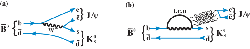
Figure 1: (a) Tree level and (b) penguin diagram examples for $\kern 1.79993pt\overline{\kern-1.79993ptB}{}^{0}$ decays into ${J\mskip-3.0mu/\mskip-2.0mu\psi\mskip 2.0mu}K^{0}_{\rm\scriptscriptstyle S}$.

The decay $\kern 1.79993pt\overline{\kern-1.79993ptB}{}^{0}\rightarrow{J\mskip-3.0mu/\mskip-2.0mu\psi\mskip 2.0mu}\pi^{+}\pi^{-}$ can occur via a Cabibbo suppressed tree level diagram, shown in Fig. 2(a), or via several penguin diagrams. An example is shown in Fig. 2(b), while others are illustrated in Ref. [19]. These decays are interesting because they can also be used to measure or limit the amount of penguin pollution. The advantage in using the decay $\kern 1.79993pt\overline{\kern-1.79993ptB}{}^{0}\rightarrow{J\mskip-3.0mu/\mskip-2.0mu\psi\mskip 2.0mu}\pi^{+}\pi^{-}$ arises because the relative amount of pollution is larger. In the allowed decays, e.g. $\kern 1.79993pt\overline{\kern-1.79993ptB}{}^{0}\rightarrow{J\mskip-3.0mu/\mskip-2.0mu\psi\mskip 2.0mu}K^{0}_{\rm\scriptscriptstyle S}$, the penguin amplitude is multiplied by a factor of $\lambda^{2}Re^{i\phi}$, where $\lambda$ is the sine of the Cabibbo angle $(\approx 0.22)$, while in the suppressed decays the factor becomes $R^{\prime}e^{i\phi^{\prime}}$, where $R$ and $R^{\prime}$, and $\phi$ and $\phi^{\prime}$ are expected to be similar in size [19]. A similar study uses the decay $B_{s}^{0}\rightarrow{J\mskip-3.0mu/\mskip-2.0mu\psi\mskip 2.0mu}K^{0}_{\rm\scriptscriptstyle S}$ [20, *Aaij:2012di, *DeBruyn:2010hh].

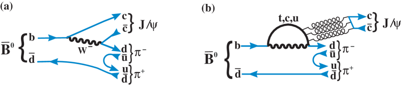
Figure 2: (a) Tree level and (b) penguin diagram for $\kern 1.79993pt\overline{\kern-1.79993ptB}{}^{0}$ decays into ${J\mskip-3.0mu/\mskip-2.0mu\psi\mskip 2.0mu}\pi^{+}\pi^{-}$.

$C\!P$ violation measurements in the ${J\mskip-3.0mu/\mskip-2.0mu\psi\mskip 2.0mu}\pi^{+}\pi^{-}$ mode utilizing $B^{0}-\kern 1.79993pt\overline{\kern-1.79993ptB}{}^{0}$ mixing determine $\sin 2\beta^{\rm eff}$ which can be compared to the well measured $\sin 2\beta$. Differences can be used to estimate the magnitude of penguin effects. Knowledge of the final state structure is the first step in this program. Such measurements on $\sin 2\beta^{\rm eff}$ have been attempted in the $\kern 1.79993pt\overline{\kern-1.79993ptB}{}^{0}$ system by using the ${J\mskip-3.0mu/\mskip-2.0mu\psi\mskip 2.0mu}\pi^{0}$ final state [23, *Aubert:2008bs, *Jung:2012pz].

In order to ascertain the viability of such $C\!P$ violation measurements we perform a full “Dalitz like” analysis of the final state. Regions in $\pi^{+}\pi^{-}$ mass that correspond to spin-0 final states would be $C\!P$ eigenstates. Final states containing vector resonances, such as the $\rho(770)$ can be analyzed in a similar manner as was done for the decay $\kern 1.79993pt\overline{\kern-1.79993ptB}{}^{0}_{s}\rightarrow{J\mskip-3.0mu/\mskip-2.0mu\psi\mskip 2.0mu}\phi$ [4, 5, 6, *Abazov:2011ry, *:2012fu].

It is also of interest to search for the $f_{0}(980)$ contribution and to obtain information concerning the mixing angle between the $f_{0}(980)$ and the $f_{0}(500)$ partners in the scalar nonet, as the latter should couple strongly to the $d\bar{d}$ system. Branching fractions for $\kern 1.79993pt\overline{\kern-1.79993ptB}{}^{0}\rightarrow{J\mskip-3.0mu/\mskip-2.0mu\psi\mskip 2.0mu}\pi^{+}\pi^{-}$ and ${J\mskip-3.0mu/\mskip-2.0mu\psi\mskip 2.0mu}\rho^{0}$ have previously been measured by the BaBar collaboration [26, *Aubert:2007xw].

In this paper the ${J\mskip-3.0mu/\mskip-2.0mu\psi\mskip 2.0mu}\pi^{+}$ and $\pi^{+}\pi^{-}$ mass spectra and decay angular distributions are used to determine the resonant and non-resonant components. This differs from a classical Dalitz plot analysis [28] because one of the particles in the final state, the ${J\mskip-3.0mu/\mskip-2.0mu\psi\mskip 2.0mu}$ meson, has spin-1 and its three decay amplitudes must be considered. We first show that there are no evident structures in the ${J\mskip-3.0mu/\mskip-2.0mu\psi\mskip 2.0mu}\pi^{+}$ invariant mass, and then model the $\pi^{+}\pi^{-}$ invariant mass with a series of resonant and non-resonant amplitudes. The data are then fitted with the coherent sum of these amplitudes. We report on the resonant structure and the $C\!P$ content of the final state.

2 Data sample and selection requirements

The data sample consists of $1.0~{}\rm fb^{-1}$ of integrated luminosity collected with the LHCb detector [29] using $pp$ collisions at a center-of-mass energy of 7 TeV. The detector is a single-arm forward spectrometer covering the pseudorapidity range $2<\eta<5$, designed for the study of particles containing $b$ or $c$ quarks. Components include a high precision tracking system consisting of a silicon-strip vertex detector surrounding the $pp$ interaction region, a large-area silicon-strip detector located upstream of a dipole magnet with a bending power of about $4{\rm\,Tm}$, and three stations of silicon-strip detectors and straw drift-tubes placed downstream. The combined tracking system has a momentum resolution $\Delta p/p$ that varies from 0.4% at 5$\mathrm{\,Ge\kern-1.00006ptV}$ to 0.6% at 100$\mathrm{\,Ge\kern-1.00006ptV}$, and an impact parameter resolution of 20$\,\upmu\rm m$ for tracks with large transverse momentum ($p_{\rm T}$) with respect to the proton beam direction. Charged hadrons are identified using two ring-imaging Cherenkov (RICH) detectors. Photon, electron and hadron candidates are identified by a calorimeter system consisting of scintillating-pad and preshower detectors, an electromagnetic calorimeter and a hadronic calorimeter. Muons are identified by a system composed of alternating layers of iron and multiwire proportional chambers. The trigger consists of a hardware stage, based on information from the calorimeter and muon systems, followed by a software stage that applies a full event reconstruction [30].

Events are triggered by a ${J\mskip-3.0mu/\mskip-2.0mu\psi\mskip 2.0mu}\!\rightarrow\mu^{+}\mu^{-}$ decay, requiring two identified muons with opposite charge, $\mbox{$p_{\rm T}$}(\mu^{\pm})$ greater than 500$\mathrm{\,Me\kern-1.00006ptV}$, an invariant mass within 120$\mathrm{\,Me\kern-1.00006ptV}$ of the ${J\mskip-3.0mu/\mskip-2.0mu\psi\mskip 2.0mu}$ mass [31], and form a vertex with a fit $\chi^{2}$ less than 16. After applying these requirements, there is a large ${J\mskip-3.0mu/\mskip-2.0mu\psi\mskip 2.0mu}$ signal over a small background [32]. Only candidates with dimuon invariant mass between $-$48$\mathrm{\,Me\kern-1.00006ptV}$ and +43$\mathrm{\,Me\kern-1.00006ptV}$ relative to the observed ${J\mskip-3.0mu/\mskip-2.0mu\psi\mskip 2.0mu}$ mass peak are selected, corresponding a window of about $\pm 3\sigma$. The requirement is asymmetric because of final state electromagnetic radiation. The two muons subsequently are kinematically constrained to the known ${J\mskip-3.0mu/\mskip-2.0mu\psi\mskip 2.0mu}$ mass.

Other requirements are imposed to isolate $\kern 1.79993pt\overline{\kern-1.79993ptB}{}^{0}$ candidates with high signal yield and minimum background. This is accomplished by combining the ${J\mskip-3.0mu/\mskip-2.0mu\psi\mskip 2.0mu}\rightarrow\mu^{+}\mu^{-}$ candidate with a pair of pion candidates of opposite charge, and then testing if all four tracks form a common decay vertex. Pion candidates are each required to have $p_{\rm T}$ greater than 250$\mathrm{\,Me\kern-1.00006ptV}$, and the scalar sum of the two transverse momenta, $\mbox{$p_{\rm T}$}(\pi^{+})+\mbox{$p_{\rm T}$}(\pi^{-})$, must be larger than 900$\mathrm{\,Me\kern-1.00006ptV}$. The impact parameter (IP) is the distance of closest approach of a track to the primary vertex (PV). To test for inconsistency with production at the PV, the IP $\chi^{2}$ is computed as the difference between the $\chi^{2}$ of the PV reconstructed with and without the considered track. Each pion must have an IP $\chi^{2}$ greater than 9. Both pions must also come from a common vertex with an acceptable $\chi^{2}$ and form a vertex with the ${J\mskip-3.0mu/\mskip-2.0mu\psi\mskip 2.0mu}$ with a $\chi^{2}$ per number of degrees of freedom (ndf) less than 10 (here ndf equals five). Pion and kaon candidates are positively identified using the RICH system. Cherenkov photons are matched to tracks, the emission angles of the photons compared with those expected if the particle is an electron, pion, kaon or proton, and a likelihood is then computed. The particle identification makes use of the logarithm of the likelihood ratio comparing two particle hypotheses (DLL). For pion selection we require DLL$(\pi-K)>-10$.

The four-track $\kern 1.79993pt\overline{\kern-1.79993ptB}{}^{0}$ candidate must have a flight distance of more than 1.5 mm, where the average decay length resolution is 0.17 mm. The angle between the combined momentum vector of the decay products and the vector formed from the positions of the PV and the decay vertex (pointing angle) is required to be less than $2.5^{\circ}$.

Events satisfying this preselection are then further filtered using a multivariate analyzer based on a Boosted Decision Tree (BDT) technique [33]. The BDT uses six variable that are chosen in a manner that does not introduce an asymmetry between either the two muons or the two pions. They are the minimum DLL($\mu-\pi$) of the $\mu^{+}$ and $\mu^{-}$, the minimum $p_{\rm T}$ of the $\pi^{+}$ and $\pi^{-}$, the minimum of the IP $\chi^{2}$ of the $\pi^{+}$ and $\pi^{-}$, the $\kern 1.79993pt\overline{\kern-1.79993ptB}{}^{0}$ vertex $\chi^{2}$, the $\kern 1.79993pt\overline{\kern-1.79993ptB}{}^{0}$ pointing angle, and the $\kern 1.79993pt\overline{\kern-1.79993ptB}{}^{0}$ flight distance. There is discrimination power between signal and background in all of these variables, especially the $\kern 1.79993pt\overline{\kern-1.79993ptB}{}^{0}$ vertex $\chi^{2}$.

The background sample used to train the BDT consists of the events in the $\kern 1.79993pt\overline{\kern-1.79993ptB}{}^{0}$ mass sideband having $5566<m({J\mskip-3.0mu/\mskip-2.0mu\psi\mskip 2.0mu}\pi^{+}\pi^{-})<5616$$\mathrm{\,Me\kern-1.00006ptV}$. The signal sample consists of two million $\kern 1.79993pt\overline{\kern-1.79993ptB}{}^{0}\rightarrow{J\mskip-3.0mu/\mskip-2.0mu\psi\mskip 2.0mu}(\rightarrow\mu^{+}\mu^{-})\pi^{+}\pi^{-}$ Monte Carlo simulated events that are generated uniformly in phase space, using Pythia [34] with a special LHCb parameter tune [35], and the LHCb detector simulation based on Geant4 [36] described in Ref. [37]. Separate samples are used to train and test the BDT. The distributions of the BDT classifier for signal and background are shown in Fig. 3. To minimize a possible bias on the signal acceptance due to the BDT, we choose a relatively loose requirement of the BDT classifier $>0.05$ which has a 96% signal efficiency and a 92% background rejection rate.

Figure 3: Distributions of the BDT classifier for both training and test samples of ${J\mskip-3.0mu/\mskip-2.0mu\psi\mskip 2.0mu}\pi^{+}\pi^{-}$ signal and background events. The signal samples are from simulation and the background samples are from data.

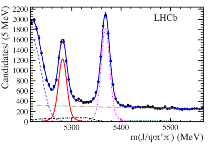
Figure 4: Invariant mass of ${J\mskip-3.0mu/\mskip-2.0mu\psi\mskip 2.0mu}\pi^{+}\pi^{-}$ combinations. The data are fitted with a double-Gaussian signal and several background functions. The (red) solid double-Gaussian function centered at 5280$\mathrm{\,Me\kern-1.00006ptV}$ is the $\kern 1.79993pt\overline{\kern-1.79993ptB}{}^{0}$ signal, the (brown) dotted line shows the combinatorial background, the (green) short-dashed shows the $B^{-}$ background, the (purple) dot-dashed line shows the contribution of $\kern 1.79993pt\overline{\kern-1.79993ptB}{}^{0}_{s}\rightarrow{J\mskip-3.0mu/\mskip-2.0mu\psi\mskip 2.0mu}\pi^{+}\pi^{-}$ decays, the (black) dot-long dashed is the sum of $\kern 1.79993pt\overline{\kern-1.79993ptB}{}^{0}_{s}\rightarrow{J\mskip-3.0mu/\mskip-2.0mu\psi\mskip 2.0mu}\eta^{\prime}(\rightarrow\rho\gamma)$ and $\kern 1.79993pt\overline{\kern-1.79993ptB}{}^{0}_{s}\rightarrow{J\mskip-3.0mu/\mskip-2.0mu\psi\mskip 2.0mu}\phi(\rightarrow\pi^{+}\pi^{-}\pi^{0})$ backgrounds, the (light blue) long-dashed is the $\kern 1.79993pt\overline{\kern-1.79993ptB}{}^{0}\rightarrow{J\mskip-3.0mu/\mskip-2.0mu\psi\mskip 2.0mu}K^{-}\pi^{+}$ reflection, and the (blue) solid line is the total.

The invariant mass of the selected ${J\mskip-3.0mu/\mskip-2.0mu\psi\mskip 2.0mu}\pi^{+}\pi^{-}$ combinations, where the dimuon pair is constrained to have the ${J\mskip-3.0mu/\mskip-2.0mu\psi\mskip 2.0mu}$ mass, is shown in Fig. 4. There are signal peaks at both the $\kern 1.79993pt\overline{\kern-1.79993ptB}{}^{0}_{s}$ and $\kern 1.79993pt\overline{\kern-1.79993ptB}{}^{0}$ masses on top of the background. Double-Gaussian functions are used to fit both signal peaks. They differ only in their mean values, which are determined by the data. The core Gaussian width is also allowed to vary, while the fraction and width ratio of the second Gaussian is fixed to that obtained in the fit of $\kern 1.79993pt\overline{\kern-1.79993ptB}{}^{0}_{s}\rightarrow{J\mskip-3.0mu/\mskip-2.0mu\psi\mskip 2.0mu}\phi$ events. (The details of the fit are given in Ref. [10].) Other components in the fit model take into account background contributions. One source is from $B^{-}\rightarrow{J\mskip-3.0mu/\mskip-2.0mu\psi\mskip 2.0mu}K^{-}$decays, which contributes when the $K^{-}$ is misidentifed as a $\pi^{-}$ and then combined with a random $\pi^{+}$; the smaller ${J\mskip-3.0mu/\mskip-2.0mu\psi\mskip 2.0mu}\pi^{-}$ mode contributes when it is combined with a random $\pi^{+}$. The next source contains $\kern 1.79993pt\overline{\kern-1.79993ptB}{}^{0}_{s}\rightarrow{J\mskip-3.0mu/\mskip-2.0mu\psi\mskip 2.0mu}\eta^{\prime}(\rightarrow\rho\gamma)$ and $\kern 1.79993pt\overline{\kern-1.79993ptB}{}^{0}_{s}\rightarrow{J\mskip-3.0mu/\mskip-2.0mu\psi\mskip 2.0mu}\phi(\rightarrow\pi^{+}\pi^{-}\pi^{0})$ decays where the $\gamma$ and the $\pi^{0}$ are ignored respectively. Finally there is a $\kern 1.79993pt\overline{\kern-1.79993ptB}{}^{0}\rightarrow{J\mskip-3.0mu/\mskip-2.0mu\psi\mskip 2.0mu}K^{-}\pi^{+}$ reflection where the $K^{-}$ is misidentified as $\pi^{-}$. Here and elsewhere charged conjugated modes are included when appropriate. The exponential combinatorial background shape is taken from same-sign combinations, that are the sum of ${J\mskip-3.0mu/\mskip-2.0mu\psi\mskip 2.0mu}\pi^{+}\pi^{+}$ and ${J\mskip-3.0mu/\mskip-2.0mu\psi\mskip 2.0mu}\pi^{-}\pi^{-}$ candidates. The shapes of the other components are taken from the simulation with their normalizations allowed to vary. The fit gives $5287\pm 112$ signal and $3212\pm 80$ background candidates within $\pm 20$$\mathrm{\,Me\kern-1.00006ptV}$ of the $\kern 1.79993pt\overline{\kern-1.79993ptB}{}^{0}$ mass peak, where a $K^{0}_{\rm\scriptscriptstyle S}$ veto, discussed later, is applied.

We use the well measured $B^{-}\rightarrow{J\mskip-3.0mu/\mskip-2.0mu\psi\mskip 2.0mu}K^{-}$ mode as a normalization channel to determine the branching fractions. To minimize the systematic uncertainty from the BDT selection, we employ a similar selection on $B^{-}\rightarrow{J\mskip-3.0mu/\mskip-2.0mu\psi\mskip 2.0mu}K^{-}$ decays after requiring the same pre-selection except for particle identification criteria on the $K^{-}$ candidates. Similar variables are used for the BDT except that the variables describing the combination of $\pi^{+}$ and $\pi^{-}$ in the ${J\mskip-3.0mu/\mskip-2.0mu\psi\mskip 2.0mu}\pi^{+}\pi^{-}$ final state are replaced by ones describing the $K^{-}$ meson. For BDT training, the signal sample uses simulated events and the background sample consists of the data events in the region $5400<m({J\mskip-3.0mu/\mskip-2.0mu\psi\mskip 2.0mu}K^{-})<5450$$\mathrm{\,Me\kern-1.00006ptV}$. The resulting invariant mass distribution of the candidates satisfying BDT classifier $>0.05$ is shown in Fig. 5. Fitting the distribution with a double-Gaussian function for the signal and linear function for the background gives $350{,}727\pm 633$ signal and $4756\pm 103$ background candidates within $\pm 20$$\mathrm{\,Me\kern-1.00006ptV}$ of the $B^{-}$ mass peak.

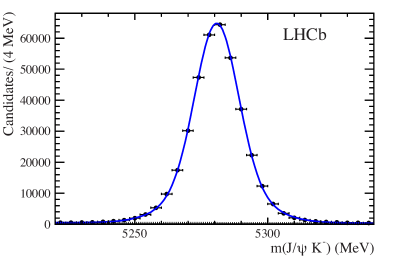
Figure 5: Invariant mass of ${J\mskip-3.0mu/\mskip-2.0mu\psi\mskip 2.0mu}K^{-}$ combinations. The data points are fitted with a double-Gaussian function for signal and a linear function for background. The dotted line shows the background, and the (blue) solid line is the total.

3 Analysis formalism

We apply a formalism similar to that used in Belle’s analysis [38] of $\kern 1.79993pt\overline{\kern-1.79993ptB}{}^{0}\rightarrow K^{-}\pi^{+}\chi_{c1}$ decays and later used in LHCb’s analysis of $\kern 1.79993pt\overline{\kern-1.79993ptB}{}^{0}_{s}\rightarrow{J\mskip-3.0mu/\mskip-2.0mu\psi\mskip 2.0mu}\pi^{+}\pi^{-}$ decays [10]. The decay $\kern 1.79993pt\overline{\kern-1.79993ptB}{}^{0}\rightarrow{J\mskip-3.0mu/\mskip-2.0mu\psi\mskip 2.0mu}\pi^{+}\pi^{-}$, with ${J\mskip-3.0mu/\mskip-2.0mu\psi\mskip 2.0mu}\rightarrow\mu^{+}\mu^{-}$, can be described by four variables. These are taken to be the invariant mass squared of ${J\mskip-3.0mu/\mskip-2.0mu\psi\mskip 2.0mu}\pi^{+}$ ($s_{12}\equiv m^{2}({J\mskip-3.0mu/\mskip-2.0mu\psi\mskip 2.0mu}\pi^{+})$), the invariant mass squared of $\pi^{+}\pi^{-}$ ($s_{23}\equiv m^{2}(\pi^{+}\pi^{-})$), where we use label 1 for ${J\mskip-3.0mu/\mskip-2.0mu\psi\mskip 2.0mu}$, 2 for $\pi^{+}$ and 3 for $\pi^{-}$, the ${J\mskip-3.0mu/\mskip-2.0mu\psi\mskip 2.0mu}$ helicity angle ($\theta_{{J\mskip-3.0mu/\mskip-2.0mu\psi\mskip 2.0mu}}$), which is the angle of the $\mu^{+}$ in the ${J\mskip-3.0mu/\mskip-2.0mu\psi\mskip 2.0mu}$ rest frame with respect to the ${J\mskip-3.0mu/\mskip-2.0mu\psi\mskip 2.0mu}$ direction in the $\kern 1.79993pt\overline{\kern-1.79993ptB}{}^{0}$ rest frame, and the angle between the ${J\mskip-3.0mu/\mskip-2.0mu\psi\mskip 2.0mu}$ and $\pi^{+}\pi^{-}$ decay planes ($\chi$) in the $\kern 1.79993pt\overline{\kern-1.79993ptB}{}^{0}$ rest frame. To improve the resolution of these variables we perform a kinematic fit constraining the $\kern 1.79993pt\overline{\kern-1.79993ptB}{}^{0}$ and ${J\mskip-3.0mu/\mskip-2.0mu\psi\mskip 2.0mu}$ masses to their nominal values [31], and recompute the final state momenta. To simplify the probability density function, we analyze the decay process after integrating over $\chi$, which eliminates several interference terms.

3.1 The decay model for $\kern 1.79993pt\overline{\kern-1.79993ptB}{}^{0}\rightarrow{J\mskip-3.0mu/\mskip-2.0mu\psi\mskip 2.0mu}\pi^{+}\pi^{-}$

The overall probability density function (PDF) given by the sum of signal, $S$, and background, $B$, functions is

$$F(s_{12},s_{23},\theta_{{J\mskip-3.0mu/\mskip-2.0mu\psi\mskip 2.0mu}})=\frac{f_{\rm sig}}{{\cal{N}}_{\rm sig}}\varepsilon(s_{12},s_{23},\theta_{{J\mskip-3.0mu/\mskip-2.0mu\psi\mskip 2.0mu}})S(s_{12},s_{23},\theta_{{J\mskip-3.0mu/\mskip-2.0mu\psi\mskip 2.0mu}})+\frac{(1-f_{\rm sig})}{{\cal{N}}_{\rm bkg}}B(s_{12},s_{23},\theta_{{J\mskip-3.0mu/\mskip-2.0mu\psi\mskip 2.0mu}}),$$ (1)

where $f_{\rm sig}$ is the fraction of the signal in the fitted region and $\varepsilon$ is the detection efficiency. The fraction of the signal is obtained from the mass fit and is fixed for the subsequent analysis. The normalization factors are given by

$${\cal{N}}_{\rm sig} = \int\!\varepsilon(s_{12},s_{23},\theta_{{J\mskip-3.0mu/\mskip-2.0mu\psi\mskip 2.0mu}})S(s_{12},s_{23},\theta_{{J\mskip-3.0mu/\mskip-2.0mu\psi\mskip 2.0mu}})\,ds_{12}ds_{23}d\cos\theta_{{J\mskip-3.0mu/\mskip-2.0mu\psi\mskip 2.0mu}},$$

$${\cal{N}}_{\rm bkg} = \int\!B(s_{12},s_{23},\theta_{{J\mskip-3.0mu/\mskip-2.0mu\psi\mskip 2.0mu}})\,ds_{12}ds_{23}d\cos\theta_{{J\mskip-3.0mu/\mskip-2.0mu\psi\mskip 2.0mu}}.$$ (2)

The event distribution for $m^{2}(\pi^{+}\pi^{-})$ versus $m^{2}({J\mskip-3.0mu/\mskip-2.0mu\psi\mskip 2.0mu}\pi^{+})$ in Fig. 6 shows obvious structure in $m^{2}(\pi^{+}\pi^{-})$. To investigate if there are visible exotic structures in the ${J\mskip-3.0mu/\mskip-2.0mu\psi\mskip 2.0mu}\pi^{+}$ system as claimed in similar decays [39], we examine the ${J\mskip-3.0mu/\mskip-2.0mu\psi\mskip 2.0mu}\pi^{+}$ mass distribution shown in Fig. 7 (a). No resonant effects are evident. Figure 7 (b) shows the $\pi^{+}\pi^{-}$ mass distribution. There is a clear peak at the $\rho(770)$ region, a small bump around 1250$\mathrm{\,Me\kern-1.00006ptV}$, but no evidence for the $f_{0}(980)$ resonance. The favored $\kern 1.79993pt\overline{\kern-1.79993ptB}{}^{0}\rightarrow{J\mskip-3.0mu/\mskip-2.0mu\psi\mskip 2.0mu}K^{0}_{\rm\scriptscriptstyle S}$ decay is mostly rejected by the $\kern 1.79993pt\overline{\kern-1.79993ptB}{}^{0}$ vertex $\chi^{2}$ selection, but about 150 such events remain. We eliminate them by excluding the candidates that have $|m(\pi^{+}\pi^{-})-m_{K^{0}_{\rm\scriptscriptstyle S}}|<$ 25$\mathrm{\,Me\kern-1.00006ptV}$, where $m_{K^{0}_{\rm\scriptscriptstyle S}}$ is the $K^{0}_{\rm\scriptscriptstyle S}$ mass [31].

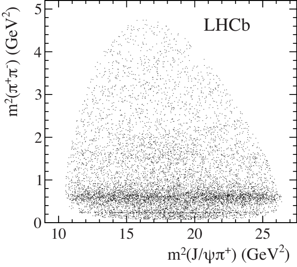
Figure 6: Distribution of $m^{2}(\pi^{+}\pi^{-})$ versus $m^{2}({J\mskip-3.0mu/\mskip-2.0mu\psi\mskip 2.0mu}\pi^{+})$ for $\kern 1.79993pt\overline{\kern-1.79993ptB}{}^{0}$ candidate decays within $\pm 20$$\mathrm{\,Me\kern-1.00006ptV}$ of the $\kern 1.79993pt\overline{\kern-1.79993ptB}{}^{0}$ mass.

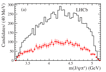
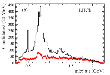
Figure 7: Distribution of (a) $m({J\mskip-3.0mu/\mskip-2.0mu\psi\mskip 2.0mu}\pi^{+})$ and (b) $m(\pi^{+}\pi^{-})$ for $\kern 1.79993pt\overline{\kern-1.79993ptB}{}^{0}\rightarrow{J\mskip-3.0mu/\mskip-2.0mu\psi\mskip 2.0mu}\pi^{+}\pi^{-}$ candidate decays within $\pm 20$$\mathrm{\,Me\kern-1.00006ptV}$ of $\kern 1.79993pt\overline{\kern-1.79993ptB}{}^{0}$ mass shown with the solid line. The (red) points with error bars show the background contribution determined from $m({J\mskip-3.0mu/\mskip-2.0mu\psi\mskip 2.0mu}\pi^{+}\pi^{-})$ fits performed in each bin.

3.1.1 The signal function

The signal function for $\kern 1.79993pt\overline{\kern-1.79993ptB}{}^{0}$ is taken to be the coherent sum over resonant states that can decay into $\pi^{+}\pi^{-}$, plus a possible non-resonant S-wave contribution

$$S(s_{12},s_{23},\theta_{{J\mskip-3.0mu/\mskip-2.0mu\psi\mskip 2.0mu}})=\sum_{\lambda=0,\pm 1}\left|\sum_{i}a^{R_{i}}_{\lambda}e^{i\phi^{R_{i}}_{\lambda}}\mathcal{A}_{\lambda}^{R_{i}}(s_{12},s_{23},\theta_{{J\mskip-3.0mu/\mskip-2.0mu\psi\mskip 2.0mu}})\right|^{2},$$ (3)

where $\mathcal{A}_{\lambda}^{R_{i}}(s_{12},s_{23},\theta_{{J\mskip-3.0mu/\mskip-2.0mu\psi\mskip 2.0mu}})$ is the amplitude of the decay via an intermediate resonance $R_{i}$ with helicity $\lambda$. Each $R_{i}$ has an associated amplitude strength $a_{\lambda}^{R_{i}}$ for each helicity state $\lambda$ and a phase $\phi_{\lambda}^{R_{i}}$. Note that the spin-0 component can only have a $\lambda=0$ term. The amplitudes for each $i$ are defined as

$$\mathcal{A}_{\lambda}^{R}(s_{12},s_{23},\theta_{{J\mskip-3.0mu/\mskip-2.0mu\psi\mskip 2.0mu}})=F_{B}^{(L_{B})}\;F_{R}^{(L_{R})}\;A_{R}(s_{23})\;\Big{(}\frac{P_{B}}{m_{B}}\Big{)}^{L_{B}}\;\Big{(}\frac{P_{R}}{\sqrt{s_{23}}}\Big{)}^{L_{R}}\;T_{\lambda}\;\Theta_{\lambda}(\theta_{{J\mskip-3.0mu/\mskip-2.0mu\psi\mskip 2.0mu}}),$$ (4)

where $P_{B}$ is the ${J\mskip-3.0mu/\mskip-2.0mu\psi\mskip 2.0mu}$ momentum in the $\kern 1.79993pt\overline{\kern-1.79993ptB}{}^{0}$ rest frame and $P_{R}$ is the momentum of either of the two pions in the dipion rest frame, $m_{B}$ is the $\kern 1.79993pt\overline{\kern-1.79993ptB}{}^{0}$ mass, $F_{B}^{(L_{B})}$ and $F_{R}^{(L_{R})}$ are the $\kern 1.79993pt\overline{\kern-1.79993ptB}{}^{0}$ meson and $R$ resonance Blatt-Weisskopf barrier factors [40], $L_{B}$ is the orbital angular momentum between the ${J\mskip-3.0mu/\mskip-2.0mu\psi\mskip 2.0mu}$ and $\pi^{+}\pi^{-}$ system, and $L_{R}$ is the orbital angular momentum in the $\pi^{+}\pi^{-}$ decay and is equal to the spin of resonance $R$ because pions have spin-0. Since the parent $\kern 1.79993pt\overline{\kern-1.79993ptB}{}^{0}$ has spin-0 and the ${J\mskip-3.0mu/\mskip-2.0mu\psi\mskip 2.0mu}$ is a vector, when the $\pi^{+}\pi^{-}$ system forms a spin-0 resonance, $L_{B}=1$ and $L_{R}=0$. For $\pi^{+}\pi^{-}$ resonances with non-zero spin, $L_{B}$ can be 0, 1 or 2 (1, 2 or 3) for $L_{R}=1(2)$ and so on. We take the lowest $L_{B}$ as the default and consider the other possibilities in the systematic uncertainty.

The Blatt-Weisskopf barrier factors $F_{B}^{(L_{B})}$ and $F_{R}^{(L_{R})}$ are

$$F^{(0)} = 1,$$

$$F^{(1)} = \frac{\sqrt{1+z_{0}}}{\sqrt{1+z}},$$ (5)

$$F^{(2)} = \frac{\sqrt{z_{0}^{2}+3z_{0}+9}}{\sqrt{z^{2}+3z+9}}.$$

For the $B$ meson $z=r^{2}P_{B}^{2}$, where the hadron scale $r$ is taken as $5.0\mathrm{\,Ge\kern-1.00006ptV}^{-1}$, and for the $R$ resonance $z=r^{2}P_{R}^{2}$ with $r$ taken as $1.5\mathrm{\,Ge\kern-1.00006ptV}^{-1}$ [41]. In both cases $z_{0}=r^{2}P_{0}^{2}$ where $P_{0}$ is the decay daughter momentum calculated at the resonance pole mass.

The angular term, $T_{\lambda}$, is obtained using the helicity formalism and is defined as

$$T_{\lambda}=d^{J}_{\lambda 0}(\theta_{\pi\pi}),$$ (6)

where $d$ is the Wigner $d$-function, $J$ is the resonance spin, $\theta_{\pi\pi}$ is the $\pi^{+}\pi^{-}$ resonance helicity angle which is defined as the angle of the $\pi^{+}$ in the $\pi^{+}\pi^{-}$ rest frame with respect to the $\pi^{+}\pi^{-}$direction in the $\kern 1.79993pt\overline{\kern-1.79993ptB}{}^{0}$ rest frame and calculated from the other variables as

$$\cos\theta_{\pi\pi}=\frac{\left[m^{2}({J\mskip-3.0mu/\mskip-2.0mu\psi\mskip 2.0mu}\pi^{+})-m^{2}({J\mskip-3.0mu/\mskip-2.0mu\psi\mskip 2.0mu}\pi^{-})\right]m(\pi^{+}\pi^{-})}{4P_{R}P_{B}m_{B}}.$$ (7)

The ${J\mskip-3.0mu/\mskip-2.0mu\psi\mskip 2.0mu}$ helicity dependent term $\Theta_{\lambda}(\theta_{{J\mskip-3.0mu/\mskip-2.0mu\psi\mskip 2.0mu}})$ is defined as

$$\Theta_{\lambda}(\theta_{{J\mskip-3.0mu/\mskip-2.0mu\psi\mskip 2.0mu}}) = \sqrt{\sin^{2}\theta_{{J\mskip-3.0mu/\mskip-2.0mu\psi\mskip 2.0mu}}}\;\;\;\;\;\;\;\;\;\text{for}\;\;\text{helicity}=0$$ (8)

$$= \sqrt{\frac{1+\cos^{2}\theta_{{J\mskip-3.0mu/\mskip-2.0mu\psi\mskip 2.0mu}}}{2}}\;\;\text{for}\;\;\text{helicity}=\pm 1.$$

The function $A_{R}(s_{23})$ describes the mass squared shape of the resonance $R$, that in most cases is a Breit-Wigner (BW) amplitude. Complications arise, however, when a new decay channel opens close to the resonant mass. The proximity of a second threshold distorts the line shape of the amplitude. This happens for the $f_{0}(980)$ resonance because the $K^{+}K^{-}$ decay channel opens. Here we use a Flatté model [42] which is described below.

The BW amplitude for a resonance decaying into two spin-0 particles, labeled as 2 and 3, is

$$A_{R}(s_{23})=\frac{1}{m^{2}_{R}-s_{23}-im_{R}\Gamma(s_{23})}~{},$$ (9)

where $m_{R}$ is the resonance pole mass, $\Gamma(s_{23})$ is its energy-dependent width that is parametrized as

$$\Gamma(s_{23})=\Gamma_{0}\left(\frac{P_{R}}{P_{0}}\right)^{2L_{R}+1}\left(\frac{m_{R}}{\sqrt{s_{23}}}\right)F^{2}_{R}~{}.$$ (10)

Here $\Gamma_{0}$ is the decay width when the invariant mass of the daughter combinations is equal to $m_{R}$.

The Flatté model is parametrized as

$$A_{R}(s_{23})=\frac{1}{m_{R}^{2}-s_{23}-im_{R}(g_{\pi\pi}\rho_{\pi\pi}+g_{KK}\rho_{KK})}.$$ (11)

The constants $g_{\pi\pi}$ and $g_{KK}$ are the $f_{0}(980)$ couplings to $\pi\pi$ and $K\kern 1.99997pt\overline{\kern-1.99997ptK}{}$ final states respectively. The $\rho$ factors account for the Lorentz-invariant phase space and are given as

$$\rho_{\pi\pi} = \frac{2}{3}\sqrt{1-\frac{4m^{2}_{\pi^{\pm}}}{m^{2}(\pi^{+}\pi^{-})}}+\frac{1}{3}\sqrt{1-\frac{4m^{2}_{\pi^{0}}}{m^{2}(\pi^{+}\pi^{-})}},$$ (12)

$$\rho_{KK} = \frac{1}{2}\sqrt{1-\frac{4m^{2}_{K^{\pm}}}{m^{2}(\pi^{+}\pi^{-})}}+\frac{1}{2}\sqrt{1-\frac{4m^{2}_{K^{0}}}{m^{2}(\pi^{+}\pi^{-})}}.$$ (13)

For non-resonant processes, the amplitude $\mathcal{A}(s_{12},s_{23},\theta_{{J\mskip-3.0mu/\mskip-2.0mu\psi\mskip 2.0mu}})$ is derived from Eq. 4, considering that the $\pi^{+}\pi^{-}$ system is S-wave (i.e. $L_{R}=0$, $L_{B}=1$) and $A_{R}(s_{23})$ is constant over the phase space $s_{12}$ and $s_{23}$. Thus, it is parametrized as

$$\mathcal{A}(s_{12},s_{23},\theta_{{J\mskip-3.0mu/\mskip-2.0mu\psi\mskip 2.0mu}})=\frac{P_{B}}{m_{B}}\sqrt{\sin^{2}\theta_{{J\mskip-3.0mu/\mskip-2.0mu\psi\mskip 2.0mu}}}.$$ (14)

3.1.2 Detection efficiency

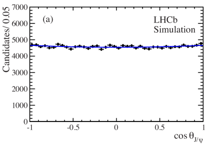
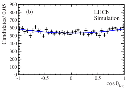
Figure 8: Distributions of $\cos\theta_{{J\mskip-3.0mu/\mskip-2.0mu\psi\mskip 2.0mu}}$ for the ${J\mskip-3.0mu/\mskip-2.0mu\psi\mskip 2.0mu}\pi^{+}\pi^{-}$ simulated sample in (a) the entire dipion mass region and (b) $\rho(770)$ region.

The detection efficiency is determined from a sample of two million $\kern 1.79993pt\overline{\kern-1.79993ptB}{}^{0}\rightarrow{J\mskip-3.0mu/\mskip-2.0mu\psi\mskip 2.0mu}(\rightarrow\mu^{+}\mu^{-})\pi^{+}\pi^{-}$ simulated events that are generated uniformly in phase space. Both $s_{12}$ and $s_{13}$ are centered at about $18.4\mathrm{\,Ge\kern-1.00006ptV}^{2}$. We model the detection efficiency using the symmetric dimensionless Dalitz plot observables

$$x=s_{12}/{\rm\mathrm{\,Ge\kern-1.00006ptV}}^{2}-18.4,~{}~{}~{}~{}{\rm and}~{}~{}~{}~{}y=s_{13}/{\rm\mathrm{\,Ge\kern-1.00006ptV}}^{2}-18.4.$$ (15)

These variables are related to $s_{23}$ since

$$s_{12}+s_{13}+s_{23}=m^{2}_{B}+m^{2}_{{J\mskip-3.0mu/\mskip-2.0mu\psi\mskip 2.0mu}}+m^{2}_{\pi^{+}}+m^{2}_{\pi^{-}}.$$ (16)

The acceptance in $\cos\theta_{{J\mskip-3.0mu/\mskip-2.0mu\psi\mskip 2.0mu}}$ is not uniform, but depends on $s_{23}$, as shown in Fig. 8. If the efficiency was independent of $s_{23}$, then the curves would have the same shape. On the other hand, no clear dependence on $s_{12}$ is seen. Thus the efficiency model can be expressed as

$$\varepsilon(s_{12},s_{23},\theta_{{J\mskip-3.0mu/\mskip-2.0mu\psi\mskip 2.0mu}})=\varepsilon_{1}(x,y)\times\varepsilon_{2}(s_{23},\theta_{{J\mskip-3.0mu/\mskip-2.0mu\psi\mskip 2.0mu}}).$$ (17)

To study the $\cos\theta_{{J\mskip-3.0mu/\mskip-2.0mu\psi\mskip 2.0mu}}$ acceptance, we fit the $\cos\theta_{{J\mskip-3.0mu/\mskip-2.0mu\psi\mskip 2.0mu}}$ distributions from simulation in 24 bins of $m^{2}(\pi^{+}\pi^{-})$ with the function

$$\varepsilon_{2}(s_{23},\theta_{{J\mskip-3.0mu/\mskip-2.0mu\psi\mskip 2.0mu}})=\frac{1+a\cos^{2}\theta_{{J\mskip-3.0mu/\mskip-2.0mu\psi\mskip 2.0mu}}}{2+2a/3},$$ (18)

giving 24 values of $a$ as a function of $m^{2}(\pi^{+}\pi^{-})$. The resultant distribution shown in Fig. 9 can be described by an exponential function

$$a(s_{23})=\exp(a_{1}+a_{2}s_{23}),$$ (19)

with $a_{1}=-1.48\pm 0.20$ and $a_{2}=(-1.45\pm 0.33)\mathrm{\,Ge\kern-1.00006ptV}^{-2}$.

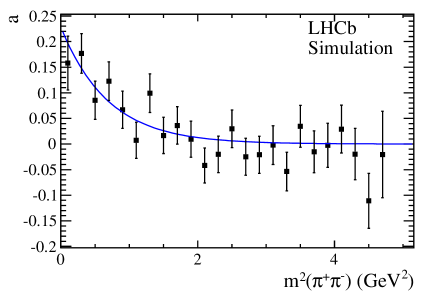
Figure 9: Exponential fit to the acceptance parameter $a(s_{12})$ used in Eq. 18.

Equation 18 is normalized with respect to $\cos\theta_{{J\mskip-3.0mu/\mskip-2.0mu\psi\mskip 2.0mu}}$. Thus, after integrating over $\cos\theta_{{J\mskip-3.0mu/\mskip-2.0mu\psi\mskip 2.0mu}}$, Eq. 17 becomes

$$\int_{-1}^{+1}\varepsilon(s_{12},s_{23},\theta_{{J\mskip-3.0mu/\mskip-2.0mu\psi\mskip 2.0mu}})d\cos\theta_{{J\mskip-3.0mu/\mskip-2.0mu\psi\mskip 2.0mu}}=\varepsilon_{1}(x,y).$$ (20)

This term of the efficiency is parametrized as a symmetric fourth order polynomial function given by

$$\varepsilon_{1}(x,y) = 1+\epsilon^{\prime}_{1}(x+y)+\epsilon^{\prime}_{2}(x+y)^{2}+\epsilon^{\prime}_{3}xy+\epsilon^{\prime}_{4}(x+y)^{3}+\epsilon^{\prime}_{5}xy(x+y)$$ (21)

$$+\epsilon^{\prime}_{6}(x+y)^{4}+\epsilon^{\prime}_{7}xy(x+y)^{2}+\epsilon^{\prime}_{8}x^{2}y^{2},$$

where the $\epsilon^{\prime}_{i}$ are the fit parameters.

Table 1: Efficiency parameters to describe the acceptance on the signal Dalitz-plot.

	Parameter	Value
	$\epsilon^{\prime}_{1}$	$0.142\pm 0.010$
	$\epsilon^{\prime}_{2}$	$0.101\pm 0.014$
	$\epsilon^{\prime}_{3}$	$0.0082\pm 0.0005$
	$\epsilon^{\prime}_{4}$	$0.027\pm 0.007$
	$\epsilon^{\prime}_{5}$	$0.0052\pm 0.0003$
	$\epsilon^{\prime}_{6}$	$0.0028\pm 0.0010$
	$\epsilon^{\prime}_{7}$	$0.00074\pm 0.00017$
	$\epsilon^{\prime}_{8}$	$-0.000105\pm 0.000008$
	$\chi^{2}/\rm ndf$	308/298

Figure 10 shows the polynomial function

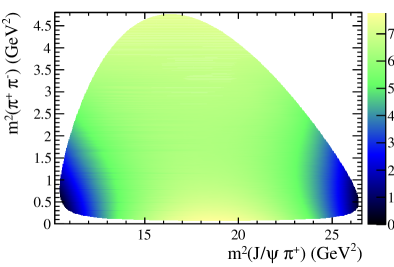
Figure 10: Parametrized detection efficiency as a function of $m^{2}(\pi^{+}\pi^{-})$ versus $m^{2}({J\mskip-3.0mu/\mskip-2.0mu\psi\mskip 2.0mu}\pi^{+})$ determined from simulation. The $z$-axis scale is arbitrary.

obtained from a fit to the Dalitz-plot distributions of simulated events. The projections of the fit are shown in Fig. 11 and the resulting parameters are given in Table 1.

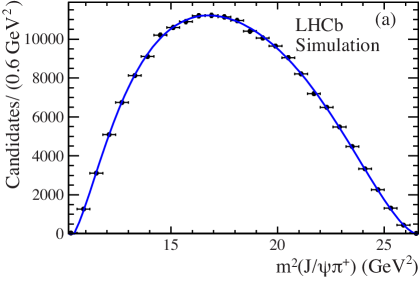
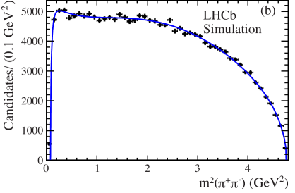
Figure 11: Projections onto (a) $m^{2}({J\mskip-3.0mu/\mskip-2.0mu\psi\mskip 2.0mu}\pi^{+})$ and (b) $m^{2}(\pi^{+}\pi^{-})$ of the simulated Dalitz plot used to determine the efficiency parameters. The points represent the simulated event distributions and the curves the projections of the polynomial fits.

3.1.3 Background composition

Backgrounds from $B$ decays into ${J\mskip-3.0mu/\mskip-2.0mu\psi\mskip 2.0mu}$ final states have already been discussed in Section 2. The main background source is combinatorial and its shape can be determined from the same-sign $\pi^{\pm}\pi^{\pm}$ combinations within $\pm 20$$\mathrm{\,Me\kern-1.00006ptV}$ of the $\kern 1.79993pt\overline{\kern-1.79993ptB}{}^{0}$ mass peak; this region also contains the small $B^{-}$ background. In addition, there is background arising from partially reconstructed $\kern 1.79993pt\overline{\kern-1.79993ptB}{}^{0}_{s}$ decays including $\kern 1.79993pt\overline{\kern-1.79993ptB}{}^{0}_{s}\rightarrow{J\mskip-3.0mu/\mskip-2.0mu\psi\mskip 2.0mu}\eta^{\prime}(\rightarrow\rho\gamma)$, $\kern 1.79993pt\overline{\kern-1.79993ptB}{}^{0}_{s}\rightarrow{J\mskip-3.0mu/\mskip-2.0mu\psi\mskip 2.0mu}\phi(\rightarrow\pi^{+}\pi^{-}\pi^{0})$, and a $\kern 1.79993pt\overline{\kern-1.79993ptB}{}^{0}\rightarrow{J\mskip-3.0mu/\mskip-2.0mu\psi\mskip 2.0mu}K^{-}\pi^{+}$ reflection, which cannot be present in same-sign combinations. We use simulated samples of inclusive $\kern 1.79993pt\overline{\kern-1.79993ptB}{}^{0}_{s}$ decays, and exclusive $\kern 1.79993pt\overline{\kern-1.79993ptB}{}^{0}\rightarrow{J\mskip-3.0mu/\mskip-2.0mu\psi\mskip 2.0mu}\kern 1.99997pt\overline{\kern-1.99997ptK}{}^{*0}(892)$ and $\kern 1.79993pt\overline{\kern-1.79993ptB}{}^{0}\rightarrow{J\mskip-3.0mu/\mskip-2.0mu\psi\mskip 2.0mu}\kern 1.99997pt\overline{\kern-1.99997ptK}{}^{*0}_{2}(1430)$ decays to model the additional backgrounds. The background fraction of each source is studied by fitting the ${J\mskip-3.0mu/\mskip-2.0mu\psi\mskip 2.0mu}\pi^{+}\pi^{-}$ candidate invariant mass distributions in bins of $m^{2}(\pi^{+}\pi^{-})$. The resulting background distribution in the $\pm 20$$\mathrm{\,Me\kern-1.00006ptV}$ $\kern 1.79993pt\overline{\kern-1.79993ptB}{}^{0}$ signal region is shown in Fig. 12. It is fit by histograms from the same-sign combinations and two additional simulations, giving a partially reconstructed $\kern 1.79993pt\overline{\kern-1.79993ptB}{}^{0}_{s}$ background of 12.8%, and a reflection background that is 5.2% of the total background.

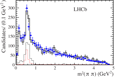
Figure 12: The $m^{2}(\pi\pi)$ distribution of background. The (black) histogram with error bars shows the same-sign data combinations with additional background from simulation, the (blue) points with error bars show the background obtained from the mass fits, the (black) dashed line is the partially reconstructed $\kern 1.79993pt\overline{\kern-1.79993ptB}{}^{0}_{s}$ background, and the (red) dotted is the misidentified $\kern 1.79993pt\overline{\kern-1.79993ptB}{}^{0}\rightarrow{J\mskip-3.0mu/\mskip-2.0mu\psi\mskip 2.0mu}K^{-}\pi^{+}$ contribution.

The background is parametrized as

$$B(s_{12},s_{23},\theta_{{J\mskip-3.0mu/\mskip-2.0mu\psi\mskip 2.0mu}})=\frac{m(\pi^{+}\pi^{-})}{2P_{R}P_{B}m_{B}}B_{1}(s_{23},\cos\theta_{\pi\pi})\times\left(1+\alpha\cos^{2}\theta_{{J\mskip-3.0mu/\mskip-2.0mu\psi\mskip 2.0mu}}\right),$$ (22)

where the first part $\frac{m(\pi^{+}\pi^{-})}{2P_{R}P_{B}m_{B}}$ converts phase space from $s_{12}$ to $\cos\theta_{\pi\pi}$, and

$$B_{1}(s_{23},\cos\theta_{\pi\pi})= \left[B_{2}(\zeta)\frac{p_{B}}{m_{B}}+\frac{b_{0}}{(m^{2}_{0}-s_{23})^{2}+m_{0}^{2}\Gamma_{0}^{2}}\right]$$ (23)

$$\times\frac{1+c_{1}q(\zeta)|\cos\theta_{\pi\pi}|+c_{4}p(\zeta)\cos^{2}\theta_{\pi\pi}}{2[1+c_{1}q(\zeta)/2+c_{4}p(\zeta)/3]}.$$

The variable $\zeta=2(s_{23}-s_{\rm min})/(s_{\rm max}-s_{\rm min})-1$, where $s_{\rm min}$ and $s_{\rm max}$ give the fit boundaries, $B_{2}(\zeta)$ is a fifth-order Chebychev polynomial with parameters $b_{i}$ ($i=1$–5), and $q(\zeta)$ and $p(\zeta)$ are both second-order Chebychev polynomials with parameters $c_{i}$ ($i$=2, 3, 5, 6), and $c_{1}$, and $c_{4}$ are free parameters. In order to better approximate the real background in the $\kern 1.79993pt\overline{\kern-1.79993ptB}{}^{0}_{s}$ signal region, the ${J\mskip-3.0mu/\mskip-2.0mu\psi\mskip 2.0mu}\pi^{\pm}\pi^{\mp}$ candidates are kinematically constrained to the $\kern 1.79993pt\overline{\kern-1.79993ptB}{}^{0}_{s}$ mass. A fit to the same-sign sample, with additional background from simulation, determines $b_{i}$, $c_{i}$, $m_{0}$ and $\Gamma_{0}$. Figure 13 shows the mass squared projections from the fit. The fitted background parameters are shown in Table 2.

The $\left(1+\alpha\cos^{2}\theta_{{J\mskip-3.0mu/\mskip-2.0mu\psi\mskip 2.0mu}}\right)$ term is a function of the ${J\mskip-3.0mu/\mskip-2.0mu\psi\mskip 2.0mu}$ helicity angle. The $\cos\theta_{{J\mskip-3.0mu/\mskip-2.0mu\psi\mskip 2.0mu}}$ distribution of background is shown in Fig. 14, and is fit with the function $1+\alpha\cos^{2}\theta_{{J\mskip-3.0mu/\mskip-2.0mu\psi\mskip 2.0mu}}$ that determines the parameter $\alpha=-0.38\pm 0.04$. We have verified that $\alpha$ is independent of $s_{23}$.

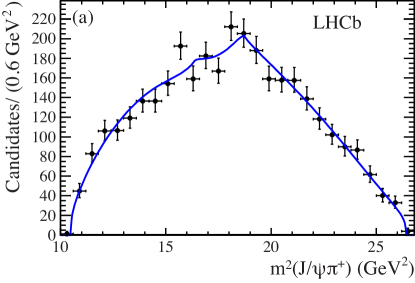
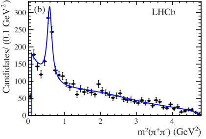
Figure 13: Projections of invariant mass squared of (a) $m^{2}({J\mskip-3.0mu/\mskip-2.0mu\psi\mskip 2.0mu}\pi^{+})$ and (b) $m^{2}(\pi^{+}\pi^{-})$ of the background Dalitz plot. The points with error bars show the same-sign combinations with additional background from simulation.

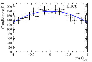
Figure 14: distribution of the background in $\cos\theta_{{J\mskip-3.0mu/\mskip-2.0mu\psi\mskip 2.0mu}}$ resulting from ${J\mskip-3.0mu/\mskip-2.0mu\psi\mskip 2.0mu}\pi^{+}\pi^{-}$ candidate mass fits in each bin of $\cos\theta_{{J\mskip-3.0mu/\mskip-2.0mu\psi\mskip 2.0mu}}$. The curve represents the fitted function $1+\alpha\cos^{2}\theta_{{J\mskip-3.0mu/\mskip-2.0mu\psi\mskip 2.0mu}}$.

Table 2: Parameters for the background model used in Eq. 23.

	Parameter	Value
	$b_{0}$	$(4.4\pm 1.2)\times 10^{-3}\mathrm{\,Ge\kern-1.00006ptV}^{4}$
	$m_{0}$	​$0.767\pm 0.005\mathrm{\,Ge\kern-1.00006ptV}$
	$\Gamma_{0}$	​$0.101\pm 0.015\mathrm{\,Ge\kern-1.00006ptV}$
	$b_{1}$	$-0.52\pm 0.07$
	$b_{2}$	$0.22\pm 0.05$
	$b_{3}$	$-0.14\pm 0.06$
	$b_{4}$	$0.11\pm 0.04$
	$b_{5}$	$-0.06\pm 0.04$
	$c_{1}$	$-0.70\pm 0.04$
	$c_{2}$	$-0.4\pm 0.3$
	$c_{3}$	$1.9\pm 0.2$
	$c_{4}$	$0.42\pm 0.03$
	$c_{5}$	$1.7\pm 0.8$
	$c_{6}$	$2.5\pm 0.8$
	$\chi^{2}/{\rm ndf}$	252/284

3.2 Fit fractions

While a complete description of the decay is given in terms of the fitted amplitudes and phases, the knowledge of the contribution of each component can be summarized by defining a fit fraction, ${\cal{F}}^{R}_{\lambda}$, as the integration of the squared amplitude of $R$ over the Dalitz plot divided by the integration of the entire signal function,

$${\cal{F}}^{R}_{\lambda}=\frac{{\int}\left|a^{R}_{\lambda}e^{i\phi^{R}_{\lambda}}\mathcal{A}_{\lambda}^{R}(s_{12},s_{23},\theta_{{J\mskip-3.0mu/\mskip-2.0mu\psi\mskip 2.0mu}})\right|^{2}ds_{12}\;ds_{23}\;d\cos\theta_{{J\mskip-3.0mu/\mskip-2.0mu\psi\mskip 2.0mu}}}{{\int}S(s_{12},s_{23},\theta_{{J\mskip-3.0mu/\mskip-2.0mu\psi\mskip 2.0mu}})~{}ds_{12}\;ds_{23}\;d\cos\theta_{{J\mskip-3.0mu/\mskip-2.0mu\psi\mskip 2.0mu}}}.$$ (24)

Note that the sum of the fit fractions over all $\lambda$ and $R$ is not necessarily unity due to the potential presence of interference between two resonances. If the Dalitz plot has more destructive interference than constructive interference, the total fit fraction will be greater than one. Interference term fractions are given by

$${\cal{F}}^{RR^{\prime}}_{\lambda}=\mathcal{R}e\left(\frac{{\int}a^{R}_{\lambda}\;a^{R^{\prime}}_{\lambda}e^{i(\phi^{R}_{\lambda}-\phi^{R^{\prime}}_{\lambda})}\mathcal{A}_{\lambda}^{R}(s_{12},s_{23},\theta_{{J\mskip-3.0mu/\mskip-2.0mu\psi\mskip 2.0mu}}){\mathcal{A}_{\lambda}^{R^{\prime}}}^{*}(s_{12},s_{23},\theta_{{J\mskip-3.0mu/\mskip-2.0mu\psi\mskip 2.0mu}})ds_{12}\;ds_{23}\;d\cos\theta_{{J\mskip-3.0mu/\mskip-2.0mu\psi\mskip 2.0mu}}}{{\int}S(s_{12},s_{23},\theta_{{J\mskip-3.0mu/\mskip-2.0mu\psi\mskip 2.0mu}})~{}ds_{12}\;ds_{23}\;d\cos\theta_{{J\mskip-3.0mu/\mskip-2.0mu\psi\mskip 2.0mu}}}\right),$$ (25)

and the sum of the two is

$$\sum_{\lambda}\left(\sum_{R}{\cal{F}}^{R}_{\lambda}+\sum_{RR^{\prime}}^{R\neq R^{\prime}}{\cal{F}}^{RR^{\prime}}_{\lambda}\right)=1.$$ (26)

Note that interference terms between different spin-$J$ states vanish, because the $d^{J}_{\lambda 0}$ angular functions in $\mathcal{A}^{R}_{\lambda}$ are orthogonal.

The statistical errors of the fit fractions depend on the statistical errors of every fitted magnitude and phase, and their correlations. Therefore, to determine the uncertainties the covariance matrix and parameter values from the fit are used to generate 500 sample parameter sets. For each set, the fit fractions are calculated. The distributions of the obtained fit fractions are described by bifurcated Gaussian functions. The widths of the Gaussians are taken as the statistical errors on the corresponding parameters. The correlations of fitted parameters are also taken into account.

4 Final state composition

4.1 Resonance models

To study the resonant structures of the decay $\kern 1.79993pt\overline{\kern-1.79993ptB}{}^{0}\rightarrow{J\mskip-3.0mu/\mskip-2.0mu\psi\mskip 2.0mu}\pi^{+}\pi^{-}$ we use those combinations with an invariant mass within $\pm 20$$\mathrm{\,Me\kern-1.00006ptV}$ of the $\kern 1.79993pt\overline{\kern-1.79993ptB}{}^{0}$ mass peak and apply a ${J\mskip-3.0mu/\mskip-2.0mu\psi\mskip 2.0mu}K^{0}_{\rm\scriptscriptstyle S}$ veto. The total number of remaining candidates is 8483, of which $3212\pm 80$ are attributed to background. Possible resonances in the decay $\kern 1.79993pt\overline{\kern-1.79993ptB}{}^{0}\rightarrow{J\mskip-3.0mu/\mskip-2.0mu\psi\mskip 2.0mu}\pi^{+}\pi^{-}$ are listed in Table 3. In addition, there could be some contribution from non-resonant $\kern 1.79993pt\overline{\kern-1.79993ptB}{}^{0}\rightarrow{J\mskip-3.0mu/\mskip-2.0mu\psi\mskip 2.0mu}\pi^{+}\pi^{-}$ decays.

Table 3: Possible resonances in the $\kern 1.79993pt\overline{\kern-1.79993ptB}{}^{0}\rightarrow{J\mskip-3.0mu/\mskip-2.0mu\psi\mskip 2.0mu}\pi^{+}\pi^{-}$ decay mode.

Resonance	Spin	Helicity	Resonance
			formalism
$f_{0}(500)$	0	0	BW
$\rho(770)$	1	$0,\pm 1$	BW
$\omega(782)$	1	$0,\pm 1$	BW
$f_{0}(980)$	0	0	Flatté
$f_{2}(1270)$	2	$0,\pm 1$	BW
$f_{0}(1370)$	0	0	BW
$\rho(1450)$	1	$0,\pm 1$	BW
$f_{0}(1500)$	0	0	BW
$\rho(1700)$	1	$0,\pm 1$	BW
$f_{0}(1710)$	0	0	BW

Table 4: Breit-Wigner resonance parameters.

Resonance	Mass ($\mathrm{\,Me\kern-1.00006ptV}$)	Width ($\mathrm{\,Me\kern-1.00006ptV}$)	Source
$f_{0}(500)$	$513\pm 32$	​$335\pm 67$	CLEO [43]
$\rho(770)$	$775.49\pm 0.34$	$149.1\pm 0.8$	PDG [31]
$\omega(782)$	$782.65\pm 0.12$	$8.49\pm 0.08$	PDG [31]
$f_{2}(1270)$	​$1275.1\pm 1.2$	$185.1_{-2.4}^{+2.9}$	PDG [31]
$f_{0}(1370)$	​$1475\pm 6$	$113\pm 11$	LHCb [10]
$\rho(1450)$	$1465\pm 25$	$400\pm 60$	PDG [31]
$f_{0}(1500)$	​$1505\pm 6$	$109\pm 7$	PDG [31]
$\rho(1700)$	$1700\pm 20$	$250\pm 100$	PDG [31]
$f_{0}(1710)$	​$1720\pm 6$	$135\pm 8$	PDG [31]

The masses and widths of the BW resonances are listed in Table 4. When used in the fit they are fixed to these values except for the parameters of the $f_{0}(500)$ resonance which are constrained by their uncertainties. Besides the mass and width, the Flatté resonance shape has two additional parameters $g_{\pi\pi}$ and $g_{KK}$, which are also fixed in the fit to values obtained in our previous Dalitz analysis of $\kern 1.79993pt\overline{\kern-1.79993ptB}{}^{0}_{s}\rightarrow{J\mskip-3.0mu/\mskip-2.0mu\psi\mskip 2.0mu}\pi^{+}\pi^{-}$ [10], where a large fraction of $\kern 1.79993pt\overline{\kern-1.79993ptB}{}^{0}_{s}$ decays are to ${J\mskip-3.0mu/\mskip-2.0mu\psi\mskip 2.0mu}f_{0}(980)$. The parameters are taken to be $m_{0}=939.9\pm 6.3$$\mathrm{\,Me\kern-1.00006ptV}$, $g_{\pi\pi}=199\pm 30$$\mathrm{\,Me\kern-1.00006ptV}$ and $g_{KK}/g_{\pi\pi}=3.0\pm 0.3$. All background and efficiency parameters are fixed in the fit.

To determine the complex amplitudes in a specific model, the data are fitted maximizing the unbinned likelihood given as

$$\mathcal{L}=\prod_{i=1}^{N}F(s^{i}_{12},s^{i}_{23},\theta^{i}_{{J\mskip-3.0mu/\mskip-2.0mu\psi\mskip 2.0mu}}),$$ (27)

where $N$ is the total number of candidates, and $F$ is the total PDF defined in Eq. 1. The PDF is constructed from the signal fraction $f_{\rm sig}$, the efficiency model $\varepsilon(s_{12},s_{23},\theta_{{J\mskip-3.0mu/\mskip-2.0mu\psi\mskip 2.0mu}})$, the background model $B(s_{12},s_{23},\theta_{{J\mskip-3.0mu/\mskip-2.0mu\psi\mskip 2.0mu}})$, and the signal model $S(s_{12},s_{23},\theta_{{J\mskip-3.0mu/\mskip-2.0mu\psi\mskip 2.0mu}})$. In order to ensure proper convergence using the maximum likelihood method, the PDF needs to be normalized. This is accomplished by first normalizing the ${J\mskip-3.0mu/\mskip-2.0mu\psi\mskip 2.0mu}$ helicity dependent part $\varepsilon(s_{23},\theta_{{J\mskip-3.0mu/\mskip-2.0mu\psi\mskip 2.0mu}})\Theta_{\lambda}(\theta_{{J\mskip-3.0mu/\mskip-2.0mu\psi\mskip 2.0mu}})$ over $\cos\theta_{{J\mskip-3.0mu/\mskip-2.0mu\psi\mskip 2.0mu}}$ by analytical integration. This integration results in additional factors as a function of $s_{23}$. We then normalize the mass dependent part multiplied by the additional factors using numerical integration over 500$\times$500 bins.

The fit determines the relative amplitude magnitudes $a_{\lambda}^{R_{i}}$ and phases $\phi_{\lambda}^{R_{i}}$ defined in Eq. 3; we choose to fix $a_{0}^{\rho(770)}$ to 1. As only relative phases are physically meaningful, one phase in each helicity grouping has to be fixed; we choose to fix those of the $f_{0}(500)$ and the $\rho(770)$ ($|\lambda|=1$) to 0. In addition, since the final state ${J\mskip-3.0mu/\mskip-2.0mu\psi\mskip 2.0mu}\pi^{+}\pi^{-}$ is a self-charge-conjugate mode and as we do not determine the $B$ flavor, the signal function is an average of $B^{0}$ and $\kern 1.79993pt\overline{\kern-1.79993ptB}{}^{0}$ decays. If we do not consider $\pi^{+}\pi^{-}$ partial waves of a higher order than D-wave, then we can express the differential decay rate derived from Eqs. 3, 4 and 8 in terms of S-, P-, and D-waves including helicity 0 and $\pm 1$

$$\frac{d\overline{\Gamma}}{dm_{\pi\pi}d\cos\theta_{\pi\pi}d\cos\theta_{{J\mskip-3.0mu/\mskip-2.0mu\psi\mskip 2.0mu}}}$$ (28)

$$= \left|{\cal A}^{s}_{S_{0}}e^{i\phi^{s}_{S_{0}}}+{\cal A}^{s}_{P_{0}}e^{i\phi^{s}_{P_{0}}}\cos\theta_{\pi\pi}+{\cal A}^{s}_{D_{0}}e^{i\phi^{s}_{D_{0}}}\left(\frac{3}{2}\cos^{2}\theta_{\pi\pi}-\frac{1}{2}\right)\right|^{2}\sin^{2}\theta_{{J\mskip-3.0mu/\mskip-2.0mu\psi\mskip 2.0mu}}$$

$$+ \left|{\cal A}^{s}_{P_{\pm 1}}e^{i\phi^{s}_{P_{\pm 1}}}\frac{1}{2}\sin\theta_{\pi\pi}+{\cal A}^{s}_{D_{\pm 1}}e^{i\phi^{s}_{D_{\pm 1}}}\sqrt{\frac{3}{2}}\sin\theta_{\pi\pi}\cos\theta_{\pi\pi}\right|^{2}\frac{1+\cos^{2}\theta_{{J\mskip-3.0mu/\mskip-2.0mu\psi\mskip 2.0mu}}}{2}$$

for $\kern 1.79993pt\overline{\kern-1.79993ptB}{}^{0}$ decays, where ${\cal A}^{s}_{k_{\lambda}}$ and $\phi^{s}_{k_{\lambda}}$ are the sum of amplitudes and reference phase for the spin-$k$ resonance group, respectively. The $B^{0}$ function for decays is similar, but $\theta_{\pi^{+}\pi^{-}}$ and $\theta_{{J\mskip-3.0mu/\mskip-2.0mu\psi\mskip 2.0mu}}$ are changed to $\pi-\theta_{\pi^{+}\pi^{-}}$ and $\pi-\theta_{{J\mskip-3.0mu/\mskip-2.0mu\psi\mskip 2.0mu}}$ respectively, as a result of using $\pi^{-}$ and $\mu^{-}$ to define the helicity angles, yielding

$$\frac{d\Gamma}{dm_{\pi\pi}d\cos\theta_{\pi\pi}d\cos\theta_{{J\mskip-3.0mu/\mskip-2.0mu\psi\mskip 2.0mu}}}$$ (29)

$$= \left|{\cal A}^{s}_{S_{0}}e^{i\phi^{s}_{S_{0}}}-{\cal A}^{s}_{P_{0}}e^{i\phi^{s}_{P_{0}}}\cos\theta_{\pi\pi}+{\cal A}^{s}_{D_{0}}e^{i\phi^{s}_{D_{0}}}\left(\frac{3}{2}\cos^{2}\theta_{\pi\pi}-\frac{1}{2}\right)\right|^{2}\sin^{2}\theta_{{J\mskip-3.0mu/\mskip-2.0mu\psi\mskip 2.0mu}}$$

$$+ \left|{\cal A}^{s}_{P_{\pm 1}}e^{i\phi^{s}_{P_{\pm 1}}}\frac{1}{2}\sin\theta_{\pi\pi}-{\cal A}^{s}_{D_{\pm 1}}e^{i\phi^{s}_{D_{\pm 1}}}\sqrt{\frac{3}{2}}\sin\theta_{\pi\pi}\cos\theta_{\pi\pi}\right|^{2}\frac{1+\cos^{2}\theta_{{J\mskip-3.0mu/\mskip-2.0mu\psi\mskip 2.0mu}}}{2}.$$

Summing Eqs. 28 and 29 results in cancellation of the interference involving the $\lambda=0$ terms for spin-1, and the $\lambda=\pm 1$ terms for spin-2, as they appear with opposite signs for $\kern 1.79993pt\overline{\kern-1.79993ptB}{}^{0}$ and $B^{0}$ decays. Therefore, we have to fix one phase in spin-1 ($\lambda=0$) group ($\phi^{s}_{P_{0}}$) and one in spin-2 ($\lambda=\pm 1$) group ($\phi^{s}_{D_{\pm 1}}$); the phases of $\rho(770)$ ($\lambda=0$) and $f_{2}(1270)$ ($\lambda=\pm 1$) are fixed to zero. The other phases in each corresponding group are relative to that of the fixed resonance.

4.2 Fit results

To find the best model, we proceed by fitting with all the possible resonances and a non-resonance (NR) component, then subsequently remove the most insignificant component one at a time. We repeat this procedure until each remaining contribution has more than 3 statistical standard deviation ($\sigma$) significance. The significance is estimated from the fit fraction divided by its statistical uncertainty. The best fit model contains six resonances, the $f_{0}(500)$, $f_{0}(980)$, $f_{2}(1270)$, $\rho(770)$, $\rho(1450)$, and $\omega(782)$.

In order to compare the different models quantitatively an estimate of the goodness of fit is calculated from three-dimensional partitions of the one angular and two mass squared variables. We use the Poisson likelihood $\chi^{2}$ [44] defined as

$$\chi^{2}=2\sum_{i=1}^{N_{\rm bin}}\left[x_{i}-n_{i}+n_{i}\text{ln}\left(\frac{n_{i}}{x_{i}}\right)\right],$$ (30)

where $n_{i}$ is the number of events in the three dimensional bin $i$ and $x_{i}$ is the expected number of events in that bin according to the fitted likelihood function. A total of 1021 bins ($N_{\rm bin}$) are used to calculate the $\chi^{2}$, based on the variables $m^{2}({J\mskip-3.0mu/\mskip-2.0mu\psi\mskip 2.0mu}\pi^{+})$, $m^{2}(\pi^{+}\pi^{-})$, and $\cos\theta_{{J\mskip-3.0mu/\mskip-2.0mu\psi\mskip 2.0mu}}$. The $\chi^{2}/\text{ndf}$ and the negative of the logarithm of the likelihood, $\rm-ln\mathcal{L}$, of the fits are given in Table 5; ndf is equal to $N_{\rm bin}-1-N_{\rm par}$, where $N_{\rm par}$ is the number of fitting parameters. The difference between the best fit results and fits with one additional component is taken as a systematic uncertainty. Figure 15 shows the best fit model projections of $m^{2}(\pi^{+}\pi^{-})$, $m^{2}({J\mskip-3.0mu/\mskip-2.0mu\psi\mskip 2.0mu}\pi^{+})$, $\cos\theta_{{J\mskip-3.0mu/\mskip-2.0mu\psi\mskip 2.0mu}}$ and $m(\pi^{+}\pi^{-})$. We calculate the fit fraction of each component using Eq. 24. For a P- or D-wave resonance, we report its total fit fraction by summing all the helicity components, and the fraction of the helicity $\lambda=0$ component. The results are listed in Table 6. Systematic uncertainties will be discussed in Section 6. Two interesting ratios of fit fractions are ($0.93_{-0.22-0.23}^{+0.37+0.47}$)% for $\omega(782)$ to $\rho(770)$, and ($9.5_{-3.4}^{+6.7}\pm 3.0$)% for $f_{0}(980)$ to $f_{0}(500)$.

The fit fractions of the interference terms are computed using Eq. 25 and listed in Table 7. Table 8 shows the resonant phases from the best fit. For the systematic uncertainty study, Table 9 shows the fit fractions of components for the best model with one additional resonance.

Table 5: Values of $\chi^{2}/\text{ndf}$ and $\rm-ln\mathcal{L}$ of different resonance models.

Resonance model	$\rm-ln\mathcal{L}$	$\chi^{2}/\text{ndf}$	Probability (%)
Best Model	35292	1058/1003	11.1
Best Model + $\rho(1700)$	35284	1045/ 999	15.0
Best Model + NR	35284	1058/1001	10.3
Best Model + $f_{0}(1370)$	35285	1047/1001	15.2
Best Model + $f_{0}(1500)$	35287	1049/1001	14.4
Best Model + $f_{0}(1710)$	35289	1052/1001	12.6

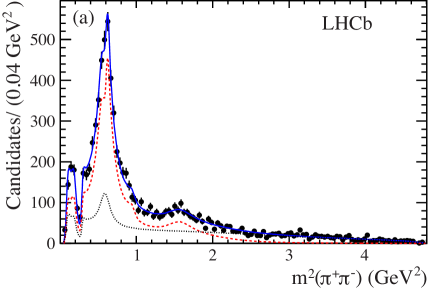
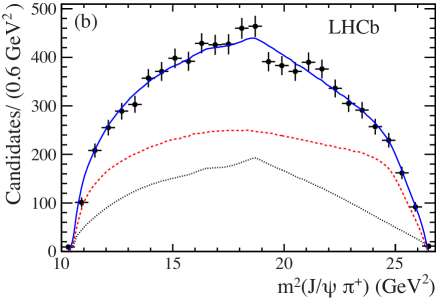
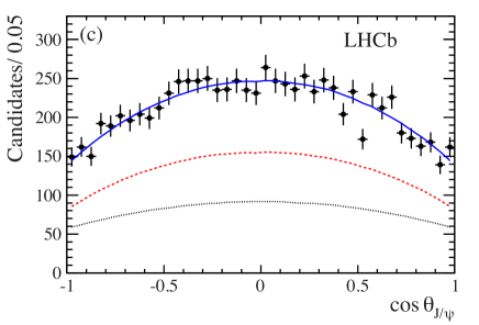
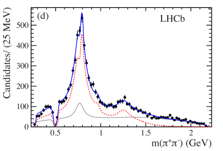
Figure 15: Dalitz fit projections of (a) $m^{2}(\pi^{+}\pi^{-})$, (b) $m^{2}({J\mskip-3.0mu/\mskip-2.0mu\psi\mskip 2.0mu}\pi^{+})$, (c) $\cos\theta_{{J\mskip-3.0mu/\mskip-2.0mu\psi\mskip 2.0mu}}$ and (d) $m(\pi^{+}\pi^{-})$ for the best model. The points with error bars are data, the signal fit is shown with a (red) dashed line, the background with a (black) dotted line, and the (blue) solid line represents the total. In (a) and (d), the shape variations near the $\rho(770)$ mass is due to $\rho(770)-\omega(782)$ interference, and the dip at the $K^{0}_{\rm\scriptscriptstyle S}$ mass [31] is due to the $K^{0}_{\rm\scriptscriptstyle S}$ veto.

Table 6: Fit fractions and significances of contributing components for the best model, as well as the fractions of the helicity $\lambda=0$ part. The significance takes into account both statistical and systematic uncertainties.

Components	Fit fraction (%)	$\lambda=0$ fraction	Significance ($\sigma$)
$\rho(770)$	$62.8_{-2.9-4.8}^{+4.8+2.8}$	$0.63\pm 0.04_{-0.03}^{+0.06}$	11.2
$\omega(782)$	$0.59_{-0.13-0.14}^{+0.23+0.27}$	$0.30^{+0.26}_{-0.18}\pm 0.05$	3.1
$f_{0}(980)$	$1.53^{+0.77+0.43}_{-0.50-0.35}$	1	2.5
$f_{2}(1270)$	$8.9\pm 1.1\pm 1.0$	$0.76\pm 0.06\pm 0.05$	5.9
$\rho(1450)$	$5.3^{+2.5+5.6}_{-1.4-0.9}$	$0.28^{+0.17+0.08}_{-0.13-0.12}$	3.2
$f_{0}(500)$	$16.2\pm 2.0^{+6.0}_{-2.0}$	1	5.7
Sum	95.2

Table 7: Interference fractions ${\cal{F}}_{\lambda}^{RR^{\prime}}$ (%) computed using Eq 25. Note that the diagonal elements are fit fractions defined in Eq 24.

		$\rho$	$\omega$	$\rho$	$f_{0}$	$f_{0}$	$f_{2}$	$\rho$	$\omega$	$\rho$	$f_{2}$
		770	782	1450	980	500	1270	770	782	1450	1270
	$|\lambda|$	0	0	0	0	0	0	1	1	1	1
$\rho(770)$	0	39.44	$-0.02$	$-0.89$	0	0	0	0	0	0	0
$\omega(782)$	0		0.18	$-0.05$	0	0	0	0	0	0	0
$\rho(1450)$	0			1.47	0	0	0	0	0	0	0
$f_{0}(980)$	0				1.53	2.08	0	0	0	0	0
$f_{0}(500)$	0					16.15	0	0	0	0	0
$f_{2}(1270)$	0						6.72	0	0	0	0
$\rho(770)$	1							23.32	0.29	0	0
$\omega(782)$	1								0.41	$-0.07$	0
$\rho(1450)$	1									3.80	0
$f_{2}(1270)$	1										2.14

Table 8: Resonant phases from the best fit.

Components	Phase (deg)
$\rho(770)$, $\lambda=0$	0 (fixed)
$\rho(770)$, $|\lambda|=1$	0 (fixed)
$\omega(782)$, $\lambda=0$	$-84\pm 31$
$\omega(782)$, $|\lambda|=1$	$-70\pm 16$
$f_{0}(980)$	$103\pm 17$
$f_{2}(1270)$, $\lambda=0$	$-87\pm 12$
$f_{2}(1270)$, $|\lambda|=1$	0 (fixed)
$\rho(1450)$, $\lambda=0$	$-162\pm 22$
$\rho(1450)$, $|\lambda|=1$	$160\pm 48$
$f_{0}(500)$	0 (fixed)

Table 9: Fit fractions (%) of contributing components for the best model with adding one additional resonance.

	Best	$+\rho(1700)$	$+f_{0}(1370)$	$+f_{0}(1500)$	$+f_{0}(1710)$	+NR
$\rho(770)$	$62.8_{-2.9}^{+4.8}$	$59.5_{-2.8}^{+3.1}$	$62.6_{-2.5}^{+3.9}$	$62.4_{-2.5}^{+4.1}$	$63.3_{-3.0}^{+5.6}$	$63.4_{-2.7}^{+3.8}$
$\omega(782)$	$0.59_{-0.13}^{+0.23}$	$0.58_{-0.15}^{+0.22}$	$0.60_{-0.15}^{+0.26}$	$0.60_{-0.15}^{+0.25}$	$0.59_{-0.15}^{+0.25}$	$0.59_{-0.14}^{+0.25}$
$f_{0}(980)$	$1.53_{-0.50}^{+0.77}$	$1.54_{-0.53}^{+0.75}$	$1.54_{-0.55}^{+0.76}$	$1.50_{-0.54}^{+0.78}$	$1.55_{-0.51}^{+0.76}$	$1.74_{-0.55}^{+0.80}$
$f_{2}(1270)$	$8.9\pm 1.1$	$8.1\pm 1.2$	$8.8\pm 1.1$	$8.8\pm 1.1$	$8.9\pm 1.1$	$8.8\pm 1.1$
$\rho(1450)$	$5.3_{-1.4}^{+2.5}$	$10.8_{-3.6}^{+5.4}$	$4.7_{-1.1}^{+1.6}$	$4.9_{-1.2}^{+1.9}$	$5.7_{-2.3}^{+4.0}$	$4.6_{-1.3}^{+2.1}$
$f_{0}(500)$	$16.2\pm 2.0$	$15.6\pm 1.9$	$16.6\pm 2.0$	$16.9\pm 2.1$	$16.3\pm 2.1$	$21.9\pm 3.8$
$\rho(1700)$	-	$3.4_{-1.5}^{+2.7}$	-	-	-	-
$f_{0}(1370)$	-	-	$1.3_{-0.5}^{+0.8}$	-	-	-
$f_{0}(1500)$	-	-	-	$1.0_{-0.4}^{+0.7}$	-	-
$f_{0}(1710)$	-	-	-	-	$0.4_{-0.2}^{+0.4}$	-
NR	-	-	-	-	-	$4.5_{-1.7}^{+2.7}$
Sum	95.2	99.6	96.2	96.0	96.7	105.5

4.3 Helicity angle distributions

We show the helicity angle distributions in the $\rho(770)$ mass region defined within one full width of the $\rho(770)$ resonance (the width values are given in Table 4) in Fig. 16. The $\cos\theta_{{J\mskip-3.0mu/\mskip-2.0mu\psi\mskip 2.0mu}}$ and $\cos\theta_{\pi\pi}$ background subtracted and efficiency corrected distributions for this mass region are presented in Fig. 17. The distributions are in good agreement with the best fit model.

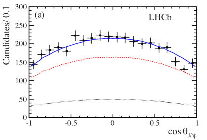
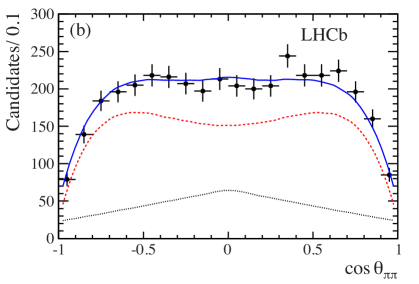
Figure 16: Helicity angle distributions of (a) $\cos\theta_{{J\mskip-3.0mu/\mskip-2.0mu\psi\mskip 2.0mu}}$ ($\chi^{2}$/ndf =15/20) and (b) $\cos\theta_{\pi\pi}$ ($\chi^{2}$/ndf =14/20) in the $\rho(770)$ mass region defined within one full width of the $\rho(770)$ mass. The points with error bars are data, the signal fit to the best model is shown with a (red) dashed line, the background with a (black) dotted line, and the (blue) solid line represents the total.

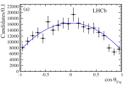
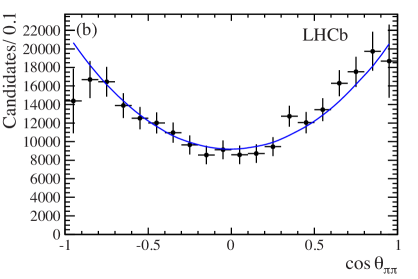
Figure 17: Background subtracted and efficiency corrected helicity distributions of (a) $\cos\theta_{{J\mskip-3.0mu/\mskip-2.0mu\psi\mskip 2.0mu}}$ ($\chi^{2}$/ndf =20/20) and (b) $\cos\theta_{\pi\pi}$ ($\chi^{2}$/ndf =13/20) in the $\rho(770)$ mass region defined within one full width of the $\rho(770)$ mass. The points with error bars are data and the solid blue lines show the fit to the best model.

5 Branching fractions

Branching fractions are measured by normalizing to the well measured decay mode $B^{-}\rightarrow{J\mskip-3.0mu/\mskip-2.0mu\psi\mskip 2.0mu}K^{-}$, which has two muons in the final state and has the same triggers as the $\kern 1.79993pt\overline{\kern-1.79993ptB}{}^{0}\rightarrow{J\mskip-3.0mu/\mskip-2.0mu\psi\mskip 2.0mu}\pi^{+}\pi^{-}$ decays. Assuming equal production of charged and neutral $B$ mesons at the LHC due to isospin symmetry, the branching fraction is calculated as

$${\cal B}(\kern 1.79993pt\overline{\kern-1.79993ptB}{}^{0}\rightarrow{J\mskip-3.0mu/\mskip-2.0mu\psi\mskip 2.0mu}\pi^{+}\pi^{-})=\frac{N_{\kern 1.25995pt\overline{\kern-1.25995ptB}{}^{0}}/\epsilon_{\kern 1.25995pt\overline{\kern-1.25995ptB}{}^{0}}}{N_{B^{-}}/\epsilon_{B^{-}}}\times{\cal B}(B^{-}\rightarrow{J\mskip-3.0mu/\mskip-2.0mu\psi\mskip 2.0mu}K^{-}),$$ (31)

where $N$ and $\epsilon$ denote the yield and total efficiency of the decay of interest. The branching fraction ${\cal B}(B^{-}\rightarrow{J\mskip-3.0mu/\mskip-2.0mu\psi\mskip 2.0mu}K^{-})=(10.18\pm 0.42)\times 10^{-4}$ is determined from an average of recent Belle [45] and BaBar [46] measurements that are corrected with respect to the reported values, which assume equal production of charged and neutral $B$ mesons at the $\Upsilon(4S)$, using the measured value of $\frac{\Gamma(B^{+}B^{-})}{\Gamma(B^{0}\kern 1.25995pt\overline{\kern-1.25995ptB}{}^{0})}=1.055\pm 0.025$ [47].

Signal efficiencies are derived from simulations including trigger, reconstruction, and event selection components. Since the efficiency to detect the ${J\mskip-3.0mu/\mskip-2.0mu\psi\mskip 2.0mu}\pi^{+}\pi^{-}$ final state is not uniform across the Dalitz plane, the efficiency is averaged according to the Dalitz model, where the best fit model is used. The $K^{0}_{\rm\scriptscriptstyle S}$ veto efficiency is also taken into account. Small corrections are applied to account for differences between the simulation and the data. We measure the kaon and pion identification efficiencies with respect to the simulation using $D^{*+}\rightarrow\pi^{+}D^{0}(\rightarrow K^{-}\pi^{+})$ events selected from data. The efficiencies are measured in bins of $p_{\rm T}$ and $\eta$ and the averages are weighted using the signal event distributions in the data. Furthermore, to ensure that the $p$ and $p_{\rm T}$ distributions of the generated $B$ mesons are correct we weight the $B^{-}$ and $\kern 1.79993pt\overline{\kern-1.79993ptB}{}^{0}$ simulation samples using $B^{-}\rightarrow{J\mskip-3.0mu/\mskip-2.0mu\psi\mskip 2.0mu}K^{-}$ and $\kern 1.79993pt\overline{\kern-1.79993ptB}{}^{0}\rightarrow{J\mskip-3.0mu/\mskip-2.0mu\psi\mskip 2.0mu}\kern 1.99997pt\overline{\kern-1.99997ptK}{}^{*0}$ data, respectively. Finally, the simulation samples are weighted with the charged tracking efficiency ratio between data and simulation in bins of $p$ and $p_{\rm T}$ of the track. The average of the weights is the correction factor. The total correction factors are below 1.04 and largely cancel between the signal and normalization channels. Multiplying the simulation efficiencies and correction factors gives the total efficiency ($1.163\pm 0.003\pm 0.017$)% for $\kern 1.79993pt\overline{\kern-1.79993ptB}{}^{0}\rightarrow{J\mskip-3.0mu/\mskip-2.0mu\psi\mskip 2.0mu}\pi^{+}\pi^{-}$ and ($3.092\pm 0.012\pm 0.038$)% for $B^{-}\rightarrow{J\mskip-3.0mu/\mskip-2.0mu\psi\mskip 2.0mu}K^{-}$, where the first uncertainty is statistical and the second is systematic.

Using $N_{B^{-}}=350{,}727\pm 633$ and $N_{\kern 1.25995pt\overline{\kern-1.25995ptB}{}^{0}}=5287\pm 112$, we measure

$${\cal B}(\kern 1.79993pt\overline{\kern-1.79993ptB}{}^{0}\rightarrow{J\mskip-3.0mu/\mskip-2.0mu\psi\mskip 2.0mu}\pi^{+}\pi^{-})=(3.97\pm 0.09\pm 0.11\pm 0.16)\times 10^{-5},$$

where the first uncertainty is statistical, the second is systematic and the third is due to the uncertainty of ${\cal B}(B^{-}\rightarrow{J\mskip-3.0mu/\mskip-2.0mu\psi\mskip 2.0mu}K^{-})$. The systematic uncertainties are discussed in Section 6. Our measured value is consistent with and more precise than the previous BaBar measurement of $(4.6\pm 0.7\pm 0.6)\times 10^{-5}$ [26].

Table 10 shows the branching fractions of resonant modes calculated by multiplying the fit fraction and the total branching fraction of $\kern 1.79993pt\overline{\kern-1.79993ptB}{}^{0}\rightarrow{J\mskip-3.0mu/\mskip-2.0mu\psi\mskip 2.0mu}\pi^{+}\pi^{-}$. Since the $f_{0}(980)$ contribution has a significance of less than 3$\sigma$ we quote also an upper limit of ${\cal{B}}\left(\kern 1.79993pt\overline{\kern-1.79993ptB}{}^{0}\rightarrow{J\mskip-3.0mu/\mskip-2.0mu\psi\mskip 2.0mu}f_{0}(980)\right)\times{\cal{B}}\left(f_{0}(980)\rightarrow\pi^{+}\pi^{-}\right)<1.1\times 10^{-6}$ at 90% confidence level (CL); this is the first such limit. The limit is calculated assuming a Gaussian distribution as the central value plus 1.28 times the addition in quadrature of the statistical and systematic uncertainties. This branching ratio is predicted to be in the range $(1-3)\times 10^{-6}$ if the $f_{0}(980)$ resonance is formed of tetra-quarks, but can be much smaller if the $f_{0}(980)$ is a standard quark anti-quark resonance [19]. Our limit is at the lower boundary of the tetra-quark prediction, and is consistent with a quark anti-quark resonance with a small mixing angle. In Section 7.2, we show that the mixing angle, describing the admixture of $s\bar{s}$ and light quarks, is less than 31^∘ at 90% CL.

The other branching fractions are consistent with and more precise than the previous measurements from BaBar [26, *Aubert:2007xw]. Using ${\cal B}(\omega\rightarrow\pi^{+}\pi^{-})=(1.53^{+0.11}_{-0.13})\%$ [31], we measure

$$\frac{{\cal B}(\kern 1.79993pt\overline{\kern-1.79993ptB}{}^{0}\rightarrow{J\mskip-3.0mu/\mskip-2.0mu\psi\mskip 2.0mu}\omega)}{{\cal B}(\kern 1.79993pt\overline{\kern-1.79993ptB}{}^{0}\rightarrow{J\mskip-3.0mu/\mskip-2.0mu\psi\mskip 2.0mu}\rho^{0})}=0.61^{+0.24+0.31}_{-0.14-0.16},$$

and

$${\cal B}(\kern 1.79993pt\overline{\kern-1.79993ptB}{}^{0}\rightarrow{J\mskip-3.0mu/\mskip-2.0mu\psi\mskip 2.0mu}\omega)=(1.5_{-0.3-0.4}^{+0.6+0.7})\times 10^{-5}.$$

This is consistent with the LHCb measurement $\frac{{\cal B}(\kern 1.25995pt\overline{\kern-1.25995ptB}{}^{0}\rightarrow{J\mskip-3.0mu/\mskip-2.0mu\psi\mskip 2.0mu}\omega)}{{\cal B}(\kern 1.25995pt\overline{\kern-1.25995ptB}{}^{0}\rightarrow{J\mskip-3.0mu/\mskip-2.0mu\psi\mskip 2.0mu}\rho^{0})}=0.89\pm 0.19^{+0.07}_{-0.13}$, using the $\omega\rightarrow\pi^{+}\pi^{-}\pi^{0}$ mode [48].

Table 10: Branching fractions for each channel. The upper limit at 90% CL is also quoted for the $f_{0}(980)$ resonance which has a significance smaller than 3$\sigma$. The first uncertainty is statistical and the second the total systematic.

Channel	${\cal B}(\kern 1.79993pt\overline{\kern-1.79993ptB}{}^{0}\rightarrow{J\mskip-3.0mu/\mskip-2.0mu\psi\mskip 2.0mu}R,R\rightarrow\pi^{+}\pi^{-})$	Upper limit of $\cal{B}$
		(at 90% CL)
$\rho(770)$	$(2.49_{-0.13-0.23}^{+0.20+0.16})\times 10^{-5}$	-
$\omega(782)$	$(2.3_{-0.5-0.6}^{+0.9+1.1})\times 10^{-7}$	-
$f_{0}(980)$	$(6.1^{+3.1+1.7}_{-2.0-1.4})\times 10^{-7}$	$<1.1\times 10^{-6}$
$f_{2}(1270)$	$(3.5\pm 0.4\pm 0.4)\times 10^{-6}$	-
$\rho(1450)$	$(2.1^{+1.0+2.2}_{-0.6-0.4})\times 10^{-6}$	-
$f_{0}(500)$	$(6.4\pm 0.8^{+2.4}_{-0.8})\times 10^{-6}$	-

6 Systematic uncertainties

Table 11: Relative systematic uncertainties on branching fractions (%).

Source	Uncertainty (%)
Tracking efficiency	1.0
Material and physical effects	2.0
Particle identification efficiency	1.0
$\kern 1.79993pt\overline{\kern-1.79993ptB}{}^{0}$ $p$ and $p_{\rm T}$ distributions	0.5
$B^{-}$ $p$ and $p_{\rm T}$ distributions	0.5
Dalitz modeling	0.6
Background modeling	0.5
Sum of above sources	2.7
$\mathcal{B}(B^{-}\rightarrow{J\mskip-3.0mu/\mskip-2.0mu\psi\mskip 2.0mu}K^{-})$	4.1
Total	4.9

The contributions to the systematic uncertainties on the branching fractions are listed in Table 11. Since the branching fractions are measured with respect to the $B^{-}\rightarrow{J\mskip-3.0mu/\mskip-2.0mu\psi\mskip 2.0mu}K^{-}$ mode, which has a different number of charged tracks than the decays of interest, a 1% systematic uncertainty is assigned due to differences in the tracking performance between data and simulation. Another 2% uncertainty is assigned because of the difference between two pions and one kaon in the final states, due to decay in flight, multiple scattering, and hadronic interactions. Small uncertainties are introduced if the simulation does not have the correct $B$ meson kinematic distributions. We are relatively insensitive to any differences in the $B$ meson $p$ and $p_{\rm T}$ distributions since we are measuring the relative rates. By varying the $p$ and $p_{\rm T}$ distributions we see at most a change of 0.5%. There is a 1.0% systematic uncertainty assigned for the relative particle identification efficiencies (0.5% per particle). These efficiencies have been corrected from those predicted in the simulation by using the data from $D^{*+}\rightarrow\pi^{+}D^{0}(\rightarrow K^{-}\pi^{+})$. A 0.6% uncertainty is included for the ${J\mskip-3.0mu/\mskip-2.0mu\psi\mskip 2.0mu}\pi^{-}\pi^{+}$ efficiency, estimated by changing the best model to that including all possible resonances. The $\kern 1.79993pt\overline{\kern-1.79993ptB}{}^{0}$ signal yield is changed by 0.5% when the shape of the combinatorial background is changed from an exponential to a linear function. The total systematic uncertainty is obtained by adding each source of systematic uncertainty in quadrature as they are uncorrelated. In addition, the largest source is $4.1\%$ due to the uncertainty of $\mathcal{B}(B^{-}\rightarrow{J\mskip-3.0mu/\mskip-2.0mu\psi\mskip 2.0mu}K^{-})$ which is quoted separately.

Table 12: Absolute systematic uncertainties on the results of the Dalitz analysis.

Item	Acceptance	Background	Fit model	Resonance parameters	Total
Fit fractions (%)
$\rho(770)$	$\pm 0.9$	${}^{+2.0}_{-3.1}$	${}^{+0.6}_{-3.2}$	$\pm 1.6$	${}^{+2.8}_{-4.8}$
$\omega(782)$	$\pm 0.08$	${}^{+0.23}_{-0.06}$	${}^{+0.11}_{-0.10}$	${}^{+0.028}_{-0.014}$	${}_{-0.14}^{+0.27}$
$f_{0}(980)$	$\pm 0.03$	${}_{-0.17}^{+0.24}$	${}^{+0.21}_{-0.18}$	${}_{-0.24}^{+0.29}$	${}^{+0.43}_{-0.35}$
$f_{2}(1270)$	$\pm 0.06$	${}_{-0.59}^{+0.45}$	${}^{+0.85}_{-0.76}$	$\pm 0.36$	$\pm 1.0$
$\rho(1450)$	$\pm 0.10$	${}^{+0.5}_{-0.6}$	${}^{+5.6}_{-0.7}$	${}^{+0.4}_{-0.3}$	${}^{+5.6}_{-0.9}$
$f_{0}(500)$	$\pm 0.4$	${}_{-0.9}^{+1.6}$	${}^{+5.7}_{-1.6}$	$\pm 0.6$	${}^{+6.0}_{-2.0}$
$\lambda=0$ fractions (%)
$\rho(770)$	$\pm 1.0$	${}_{-2.0}^{+1.7}$	${}^{+4.9}_{-1.5}$	$\pm 2.1$	${}^{+5.7}_{-3.4}$
$\omega(782)$	$\pm 1.5$	${}_{-1.8}^{+3.5}$	${}^{+2.8}_{-3.5}$	${}_{-1.7}^{+1.2}$	${}^{+4.9}_{-4.5}$
$f_{2}(1270)$	$\pm 0.3$	$\pm 2.4$	${}^{+3.7}_{-3.4}$	$\pm 1.5$	$\pm 4.5$
$\rho(1450)$	$\pm 0.9$	${}_{-8.4}^{+4.8}$	${}^{+5.5}_{-5.1}$	${}^{+4.2}_{-6.1}$	${}^{+8.4}_{-11.6}$
Ratio of fit fractions (%)
$\omega(782)/\rho(770)$	$\pm 0.13$	${}_{-0.11}^{+0.41}$	${}_{-0.16}^{+0.18}$	${}_{-0.022}^{+0.034}$	${}^{+0.47}_{-0.23}$
$f_{0}(980)/f_{0}(500)$	$\pm 0.3$	${}^{+1.5}_{-1.1}$	${}^{+1.0}_{-2.1}$	${}_{-1.8}^{+2.2}$	$\pm 3.0$

The sources of the systematic uncertainties on the results of the Dalitz plot analysis are summarized in Table 12. For the uncertainties due to the acceptance or background modeling, we repeat the data fit 100 times where the parameters of acceptance or background modeling are generated according to the corresponding covariance matrix. We also study the acceptance function by changing the minimum IP $\chi^{2}$ requirement from 9 to 12.5 on both of the pion candidates. As shown previously [10], this increases the $\chi^{2}$ of the fit to the angular distributions by one unit. The acceptance function is then applied to the data with the original minimum IP $\chi^{2}$ selection of 9, and the likelihood fit is redone and the uncertainties are estimated by comparing the results with the best fit model. The larger of the two variations is taken as uncertainty due to the acceptance.

We study the effect of ignoring the experimental mass resolution in the fit by comparing fits between different pseudo-experiments with and without the resolution included. As the widths of the resonances we consider are much larger than the mass resolution, we find that the effects are negligible except for the $\omega(782)$ resonance whose fit fraction is underestimated by ($0.09\pm 0.08$)%. Thus, we apply a $0.09\%$ correction to the $\omega(782)$ fraction and assign an additional $\pm 0.08\%$ in the acceptance systematic uncertainty. The results shown in the previous sections already include this correction.

In the default fit, the signal fraction $f_{\rm sig}=0.621\pm 0.009$, defined in Eq. 1 is fixed; we vary its value within its error to estimate the systematic uncertainty. The change is added in quadrature with the background modeling uncertainties.

The uncertainties due to the fit model include adding each resonance that is listed in Table 4 but not used in the best model, changing the default values of $L_{B}$ in P- and D-wave cases, varying the hadron scale $r$ parameters for the $B$ meson and $R$ resonance to $3.0\mathrm{\,Ge\kern-1.00006ptV}^{-1}$ for both, replacing the $f_{0}(500)$ model by a Zhou and Bugg function [49, 50] and using the alternate Gounaris and Sakurai model [51] for $\rho$ resonances. Then the largest variations among those changes are assigned as the systematic uncertainties for modeling (see Table 12).

Finally, we repeat the data fit by varying the mass and width of resonances (see Table 4) within their errors one at a time, and add the changes in quadrature.

7 Further results and implications

7.1 Resonant structure

The largest intermediate state in $\kern 1.79993pt\overline{\kern-1.79993ptB}{}^{0}\rightarrow{J\mskip-3.0mu/\mskip-2.0mu\psi\mskip 2.0mu}\pi^{+}\pi^{-}$ decays is the ${J\mskip-3.0mu/\mskip-2.0mu\psi\mskip 2.0mu}\rho(770)$ mode. Beside the $\rho(770)$, significant $f_{2}(1270)$ and $f_{0}(500)$ contributions are also seen. The smaller $\omega(782)$ and $\rho(1450)$ resonances have 3.1$\sigma$ and 3.2$\sigma$ significances respectively, including systematic uncertainties. The systematic uncertainties reduce the significance of the $f_{0}(980)$ to below $3\sigma$. Replacing the $f_{0}(500)$ by a non-resonant component increases $-\ln{\cal L}$ by 117, and worsens the $\chi^{2}$ by 192 with the same ndf resulting in a fit confidence level of $1.8\times 10^{-7}$. Thus the $f_{0}(500)$ state is firmly established in $\kern 1.79993pt\overline{\kern-1.79993ptB}{}^{0}\rightarrow{J\mskip-3.0mu/\mskip-2.0mu\psi\mskip 2.0mu}\pi^{+}\pi^{-}$ decays.

As discussed in the introduction, a region with only S- and P-waves is preferred for measuring $\sin 2\beta^{\rm eff}$. The best fit model demonstrates that the mass region within $\pm 149$$\mathrm{\,Me\kern-1.00006ptV}$ (one full width) of the $\rho(770)$ mass contains only $(0.72\pm 0.09)\%$ D-wave contribution, thus this region can be used for a clean $C\!P$ measurement. The S-wave in this region is (11.9$\pm$1.7)%, where the fraction is the sum of individual fit fractions and the interference.

7.2 Mixing angle between $f_{0}(980)$ and $f_{0}(500)$

The scalar nonet is quite an enigma. The mysteries are summarized in Ref. [52], and in the “Note on scalar mesons” in the PDG [31]. Let us contrast the masses of the lightest vector mesons with those of the scalars, listed in Table 13.

Table 13: Masses of light vector and scalar resonances. All values are taken from [31], except for the $f_{0}(500)$ [43].

Isospin	Vector particle	Vector mass ($\mathrm{\,Me\kern-1.00006ptV}$)	Scalar particle	Scalar mass ($\mathrm{\,Me\kern-1.00006ptV}$)
0	$\omega$	783	$f_{0}(500)$	513
1	$\rho$	776	$a_{0}$	980
1/2	$K^{*}$	980	$\kappa$	800
0	$\phi$	1020	$f_{0}$	980

For the vector particles, the $\omega$ and $\rho$ masses are nearly degenerate and the masses increase as the $s$-quark content increases. For the scalar particles, however, the mass dependence differs in several ways which requires an explanation. Some authors introduce the concept of $q\bar{q}q\bar{q}$ states or superpositions of the four-quark state with the $q\bar{q}$ state. In either case, the $I=0$ $f_{0}(500)$ and the $f_{0}(980)$ are thought to be mixtures of the underlying states whose mixing angle has been estimated previously (see Ref. [19] and references contained therein).

The mixing is parameterized by a 2$\times$2 rotation matrix characterized by the angle $\varphi_{m}$, giving in our case

$$|f_{0}(980)\rangle = \;\;\;\cos\varphi_{m}|s\bar{s}\rangle+\sin\varphi_{m}|n\bar{n}\rangle$$

$$|f_{0}(500)\rangle = -\sin\varphi_{m}|s\bar{s}\rangle+\cos\varphi_{m}|n\bar{n}\rangle,$$

$${\rm where~{}}|n\bar{n}\rangle \equiv \frac{1}{\sqrt{2}}\left(|u\bar{u}\rangle+|d\bar{d}\rangle\right).$$ (32)

In this case only the $|d\bar{d}\rangle$ part of the $|n\bar{n}\rangle$ wave function contributes (see Fig. 2). Thus we have

$$\tan^{2}\varphi_{m}=\frac{{\cal{B}}\left(\kern 1.79993pt\overline{\kern-1.79993ptB}{}^{0}\rightarrow{J\mskip-3.0mu/\mskip-2.0mu\psi\mskip 2.0mu}f_{0}(980)\right)}{{\cal{B}}\left(\kern 1.79993pt\overline{\kern-1.79993ptB}{}^{0}\rightarrow{J\mskip-3.0mu/\mskip-2.0mu\psi\mskip 2.0mu}f_{0}(500)\right)}\frac{\Phi(500)}{\Phi(980)},$$ (33)

where the $\Phi$ terms denote the phase space factors. The phase space in this pseudoscalar to vector-pseudoscalar decay is proportional to the cube of the $f_{0}$ three-momentum. Taking the average of the momentum dependent phase space over the resonant line shapes results in the ratio of phase space factors $\frac{\Phi(500)}{\Phi(980)}$ being equal to 1.25.

Using the data shown in Table 10 we determine the ratio of branching fractions for both resonances resulting in the $\pi^{+}\pi^{-}$ final state as

$$\frac{{\cal{B}}\left(\kern 1.79993pt\overline{\kern-1.79993ptB}{}^{0}\rightarrow{J\mskip-3.0mu/\mskip-2.0mu\psi\mskip 2.0mu}f_{0}(980)\right)\times{\cal{B}}\left(f_{0}(980)\rightarrow\pi^{+}\pi^{-}\right)}{{\cal{B}}\left(\kern 1.79993pt\overline{\kern-1.79993ptB}{}^{0}\rightarrow{J\mskip-3.0mu/\mskip-2.0mu\psi\mskip 2.0mu}f_{0}(500)\right)\times{\cal{B}}\left(f_{0}(500)\rightarrow\pi^{+}\pi^{-}\right)}=(9.5^{+6.7}_{-3.4}\pm 3.0)\%.$$

This value must be corrected for the individual branching fractions of the $f_{0}$ resonances into the $\pi^{+}\pi^{-}$ final state.

BaBar has measured $\frac{{\cal{B}}\left(f_{0}(980)\rightarrow K^{+}K^{-}\right)}{{\cal{B}}\left(f_{0}(980)\rightarrow\pi^{+}\pi^{-}\right)}=0.69\pm 0.32$ using $B\rightarrow KKK$ and $B\rightarrow K\pi\pi$ decays [53]. BES obtained relative branching ratios using $\psi(2S)\rightarrow\gamma\chi_{c0}$ decays where the $\chi_{c0}\rightarrow f_{0}(980)f_{0}(980)$, and either both $f_{0}(980)$ candidates decay into $\pi^{+}\pi^{-}$ or one into $\pi^{+}\pi^{-}$ and the other into $K^{+}K^{-}$ pairs [54, *Ablikim:2005kp]. From their results we obtain $\frac{{\cal{B}}\left(f_{0}(980)\rightarrow K^{+}K^{-}\right)}{{\cal{B}}\left(f_{0}(980)\rightarrow\pi^{+}\pi^{-}\right)}=0.25^{+0.17}_{-0.11}$[56]. Averaging the two measurements gives

$$\frac{{\cal{B}}\left(f_{0}(980)\rightarrow K^{+}K^{-}\right)}{{\cal{B}}\left(f_{0}(980)\rightarrow\pi^{+}\pi^{-}\right)}=0.35_{-0.14}^{+0.15}\,.$$ (34)

Assuming that the $\pi\pi$ and $KK$ decays are dominant we obtain

$${\cal{B}}\left(f_{0}(980)\rightarrow\pi^{+}\pi^{-}\right)=\left(46\pm 6\right)\%,$$ (35)

where we have assumed that the only other decays are to $\pi^{0}\pi^{0}$, half of the $\pi^{+}\pi^{-}$ rate, and to neutral kaons, taken equal to charged kaons. We use ${\cal{B}}\left(f_{0}(500)\rightarrow\pi^{+}\pi^{-}\right)=\frac{2}{3}$, which results from isospin Clebsch-Gordon coefficients, and assuming that the only decays are into two pions. Since we have only an upper limit on the ${J\mskip-3.0mu/\mskip-2.0mu\psi\mskip 2.0mu}f_{0}(980)$ final state, we will only find an upper limit on the mixing angle, so if any other decay modes of the $f_{0}(500)$ ($f_{0}(980)$) exist, they would make the limit more (less) stringent. Our limit then is

$$\tan^{2}\varphi_{m}=\frac{{\cal{B}}\left(\kern 1.79993pt\overline{\kern-1.79993ptB}{}^{0}\rightarrow{J\mskip-3.0mu/\mskip-2.0mu\psi\mskip 2.0mu}f_{0}(980)\right)}{{\cal{B}}\left(\kern 1.79993pt\overline{\kern-1.79993ptB}{}^{0}\rightarrow{J\mskip-3.0mu/\mskip-2.0mu\psi\mskip 2.0mu}f_{0}(500)\right)}\frac{\Phi(500)}{\Phi(980)}<0.35~{}{\rm at~{}90\%~{}confidence~{}level},$$

which translates into a limit

$$|\varphi_{m}|<31^{\circ}~{}{\rm at~{}90\%~{}confidence~{}level}.$$

Various mixing angle measurements have been derived in the literature and summarized in Ref. [19]. There are a wide range of values including: (a) using $D_{s}^{+}\rightarrow\pi^{+}\pi^{+}\pi^{-}$ transitions which give a range $35^{\circ}<|\varphi_{m}|<55^{\circ}$, (b) using radiative decays where two solutions were found either $\varphi_{m}=4^{\circ}\pm 3^{\circ}$ or $136^{\circ}\pm 6^{\circ}$, (c) using resonance decays from both $\phi\rightarrow\gamma\pi^{0}\pi^{0}$ and ${J\mskip-3.0mu/\mskip-2.0mu\psi\mskip 2.0mu}\rightarrow\omega\pi\pi$ where a value of $\varphi_{m}\simeq 20^{\circ}$ was found, (d) using the $D^{\pm}$ and $D_{s}^{\pm}$ decays into $f_{0}(980)\pi^{\pm}$ and $f_{0}(980)K^{\pm}$ where values of $\varphi_{m}=31^{\circ}\pm 5^{\circ}$ or $42^{\circ}\pm 7^{\circ}$ were found.

8 Conclusions

We have studied the resonance structure of $\kern 1.79993pt\overline{\kern-1.79993ptB}{}^{0}\rightarrow{J\mskip-3.0mu/\mskip-2.0mu\psi\mskip 2.0mu}\pi^{+}\pi^{-}$ using a modified Dalitz plot analysis where we also include the decay angle of the ${J\mskip-3.0mu/\mskip-2.0mu\psi\mskip 2.0mu}$ meson. The decay distributions are formed from a series of final states described by individual $\pi^{+}\pi^{-}$ interfering decay amplitudes. The largest component is the $\rho(770)$ resonance. The data are best described by adding the $f_{2}(1270)$, $f_{0}(500)$, $\omega(782)$, $\rho(1450)$ and $f_{0}(980)$ resonances, where the $f_{0}(980)$ resonance contributes less than $3\sigma$ significance. The results are listed in Table 6.

We set an upper limit ${\cal{B}}\left(\kern 1.79993pt\overline{\kern-1.79993ptB}{}^{0}\rightarrow{J\mskip-3.0mu/\mskip-2.0mu\psi\mskip 2.0mu}f_{0}(980)\right)\times{\cal{B}}\left(f_{0}(980)\rightarrow\pi^{+}\pi^{-}\right)<1.1\times 10^{-6}$ at 90% confidence level that favors somewhat a quark anti-quark interpretation of the $f_{0}(980)$ resonance. We also have firmly established the existence of the ${J\mskip-3.0mu/\mskip-2.0mu\psi\mskip 2.0mu}f_{0}(500)$ intermediate resonant state in $\kern 1.79993pt\overline{\kern-1.79993ptB}{}^{0}$ decays, and limit the absolute value of the mixing angle between the two lightest scalar states to be less than $31^{\circ}$ at 90% confidence level.

Our six-resonance best fit shows that the mass region within one full width of the $\rho(770)$ contains mostly P-wave, $(11.9\pm 1.7)$% S-wave, and only $(0.72\pm 0.09)$% D-wave. Thus this region can be used to perform $C\!P$ violation measurements, as the S- and P-wave components can be treated in the same manner as in the analysis of $\kern 1.79993pt\overline{\kern-1.79993ptB}{}^{0}_{s}\rightarrow{J\mskip-3.0mu/\mskip-2.0mu\psi\mskip 2.0mu}\phi$ [4, 5, 6, *Abazov:2011ry, *:2012fu]. The measured value of the asymmetry can be compared to that found in other modes such as $\kern 1.79993pt\overline{\kern-1.79993ptB}{}^{0}\rightarrow{J\mskip-3.0mu/\mskip-2.0mu\psi\mskip 2.0mu}\kern 1.99997pt\overline{\kern-1.99997ptK}{}^{0}$ in order to ascertain the possible effects due to penguin amplitudes.

The measured branching ratio is

$${\cal B}(\kern 1.79993pt\overline{\kern-1.79993ptB}{}^{0}\rightarrow{J\mskip-3.0mu/\mskip-2.0mu\psi\mskip 2.0mu}\pi^{+}\pi^{-})=(3.97\pm 0.09\pm 0.11\pm 0.16)\times 10^{-5},$$

where the first uncertainty is statistical, the second is systematic and the third is due to the uncertainty of ${\cal B}(B^{-}\rightarrow{J\mskip-3.0mu/\mskip-2.0mu\psi\mskip 2.0mu}K^{-})$. The largest contribution is the ${J\mskip-3.0mu/\mskip-2.0mu\psi\mskip 2.0mu}\rho(770)$ mode with a branching fraction of $(2.49_{-0.13-0.23}^{+0.20+0.16})\times 10^{-5}$.

References

- [1] BaBar collaboration, B. Aubert et al., Measurement of time-dependent asymmetry in decays, Phys. Rev. D79 (2009) 072009, arXiv:0902.1708
- [2] Belle collaboration, I. Adachi et al., Precise measurement of the CP violation parameter in decays, Phys. Rev. Lett. 108 (2012) 171802, arXiv:1201.4643
- [3] LHCb collaboration, R. Aaij et al., Measurement of the time-dependent asymmetry in decays, arXiv:1211.6093
- [4] LHCb collaboration, R. Aaij et al., Tagged time-dependent angular analysis of decays at LHCb, LHCb-CONF-2012-002
- [5] LHCb collaboration, R. Aaij et al., Measurement of the CP-violating phase in the decay , Phys. Rev. Lett. 108 (2012) 101803, arXiv:1112.3183
- [6] CDF collaboration, T. Aaltonen et al., Measurement of the Bottom-strange meson mixing phase in the full CDF data set, Phys. Rev. Lett. 109 (2012) 171802, arXiv:1208.2967
- [7] D0 collaboration, V. M. Abazov et al., Measurement of the CP-violating phase using the flavor-tagged decay in 8 fb-1 of collisions, Phys. Rev. D85 (2012) 032006, arXiv:1109.3166
- [8] ATLAS collaboration, G. Aad et al., Time-dependent angular analysis of the decay and extraction of and the -violating weak phase by ATLAS, JHEP 1212 (2012) 072, arXiv:1208.0572
- [9] LHCb collaboration, R. Aaij et al., Measurement of the CP-violating phase in decays, Phys. Lett. B713 (2012) 378, arXiv:1204.5675
- [10] LHCb collaboration, R. Aaij et al., Analysis of the resonant components in , Phys. Rev. D86 (2012) 052006, arXiv:1204.5643
- [11] S. Stone and L. Zhang, S-waves and the measurement of CP violating phases in decays, Phys. Rev. D79 (2009) 074024, arXiv:0812.2832
- [12] A. Lenz, Theoretical update of -mixing and lifetimes, arXiv:1205.1444
- [13] H.-n. Li and S. Mishima, Penguin pollution in the decay, JHEP 0703 (2007) 009, arXiv:hep-ph/0610120
- [14] H. Boos, T. Mannel, and J. Reuter, The Gold plated mode reexamined: and in the standard model, Phys. Rev. D70 (2004) 036006, arXiv:hep-ph/0403085
- [15] M. Ciuchini, M. Pierini, and L. Silvestrini, Effect of penguin operators in the asymmetry, Phys. Rev. Lett. 95 (2005) 221804, arXiv:hep-ph/0507290
- [16] B. Bhattacharya, A. Datta, and D. London, Reducing penguin pollution, arXiv:1209.1413
- [17] R. Fleischer, Extracting from and , Eur. Phys. J. C10 (1999) 299, arXiv:hep-ph/9903455
- [18] S. Faller, R. Fleischer, and T. Mannel, Precision Physics with at the LHC: The Quest for New Physics, Phys. Rev. D79 (2009) 014005, arXiv:0810.4248
- [19] R. Fleischer, R. Knegjens, and G. Ricciardi, Anatomy of , Eur. Phys. J. C71 (2011) 1832, arXiv:1109.1112
- [20] CDF collaboration, T. Aaltonen et al., Observation of and decays, Phys. Rev. D83 (2011) 052012, arXiv:1102.1961
- [21] LHCb collaboration, R. Aaij et al., Measurement of the branching fraction, Phys. Lett. B713 (2012) 172, arXiv:1205.0934
- [22] K. De Bruyn, R. Fleischer, and P. Koppenburg, Extracting gamma and penguin topologies through Violation in , Eur. Phys. J. C70 (2010) 1025, arXiv:1010.0089
- [23] Belle Collaboration, S. Lee et al., Improved measurement of time-dependent CP violation in , Phys. Rev. D77 (2008) 071101, arXiv:0708.0304
- [24] BaBar Collaboration, B. Aubert et al., Evidence for CP violation in decays, Phys. Rev. Lett. 101 (2008) 021801, arXiv:0804.0896
- [25] M. Jung, Recent topics in violation, PoS HQL2012 (2012) 037, arXiv:1208.1286
- [26] BaBar collaboration, B. Aubert et al., A measurement of the branching fraction, Phys. Rev. Lett. 90 (2003) 091801, arXiv:hep-ex/0209013
- [27] BaBar collaboration, B. Aubert et al., Branching fraction and charge asymmetry measurements in decays, Phys. Rev. D76 (2007) 031101, arXiv:0704.1266
- [28] R. Dalitz, On the analysis of -meson data and the nature of the -meson, Phil. Mag. 44 (1953) 1068
- [29] LHCb collaboration, A. Alves Jr. et al., The LHCb detector at the LHC, JINST 3 (2008) S08005
- [30] R. Aaij et al., The LHCb trigger and its performance, arXiv:1211.3055
- [31] Particle Data Group, J. Beringer et al., Review of particle physics, Phys. Rev. D86 (2012) 010001, http://pdg.lbl.gov/
- [32] LHCb collaboration, R. Aaij et al., First observation of decays, Phys. Lett. B698 (2011) 115, arXiv:1102.0206
- [33] L. Breiman, J. H. Friedman, R. A. Olshen, and C. J. Stone, Classification and regression trees, Wadsworth international group, Belmont, California, USA, 1984
- [34] T. Sjöstrand, S. Mrenna, and P. Skands, PYTHIA 6.4 physics and manual, JHEP 05 (2006) 026, arXiv:hep-ph/0603175
- [35] I. Belyaev et al., Handling of the generation of primary events in Gauss, the LHCb simulation framework, Nuclear Science Symposium Conference Record (NSS/MIC) IEEE (2010) 1155
- [36] GEANT4 collaboration, S. Agostinelli et al., GEANT4: A simulation toolkit, Nucl. Instrum. Meth. A506 (2003) 250
- [37] M. Clemencic et al., The LHCb simulation application, Gauss: design, evolution and experience, Journal of Physics: Conference Series 331 (2011), no. 3 032023
- [38] Belle collaboration, R. Mizuk et al., Observation of two resonance-like structures in the mass distribution in exclusive decays, Phys. Rev. D78 (2008) 072004, arXiv:0806.4098
- [39] Belle collaboration, R. Mizuk et al., Dalitz analysis of decays and the , Phys. Rev. D80 (2009) 031104, arXiv:0905.2869
- [40] J. M. Blatt and V. F. Weisskopf, Theoretical Nuclear Physics, Wiley/Springer-Verlag (1952)
- [41] CLEO collaboration, S. Kopp et al., Dalitz analysis of the decay , Phys. Rev. D63 (2001) 092001, arXiv:hep-ex/0011065
- [42] S. M. Flatté, On the nature of mesons, Phys. Lett. B63 (1976) 228
- [43] CLEO collaboration, H. Muramatsu et al., Dalitz analysis of , Phys. Rev. Lett. 89 (2002) 251802, arXiv:hep-ex/0207067
- [44] S. Baker and R. D. Cousins, Clarification of the use of and likelihood functions in fits to histograms, Nucl. Instrum. Meth. 221 (1984) 437
- [45] Belle collaboration, K. Abe et al., Measurement of branching fractions and charge asymmetries for two-body B meson decays with charmonium, Phys. Rev. D67 (2003) 032003, arXiv:hep-ex/0211047
- [46] BaBar collaboration, B. Aubert et al., Measurement of branching fractions and charge asymmetries for exclusive decays to charmonium, Phys. Rev. Lett. 94 (2005) 141801, arXiv:hep-ex/0412062
- [47] Heavy Flavor Averaging Group, Y. Amhis et al., Averages of b-hadron, c-hadron, and tau-lepton properties as of early 2012, arXiv:1207.1158
- [48] LHCb collaboration, R. Aaij et al., Evidence for the decay and measurement of the relative branching fractions of meson decays to and , Nucl. Phys. B867 (2013) 547, arXiv:1210.2631
- [49] D. Bugg, Comments on the and , Phys. Lett. B572 (2003) 1
- [50] BES collaboration, M. Ablikim et al., The pole in , Phys. Lett. B598 (2004) 149, arXiv:hep-ex/0406038
- [51] G. J. Gounaris and J. J. Sakurai, Finite-width corrections to the vector-mesion-dominance prediction for , Phys. Rev. Lett. 21 (1968) 244
- [52] J. Schechter, Testing a model for the puzzling spin 0 mesons, arXiv:1202.3176
- [53] BaBar collaboration, B. Aubert et al., Dalitz plot analysis of the decay , Phys. Rev. D74 (2006) 032003, arXiv:hep-ex/0605003
- [54] BES collaboration, M. Ablikim et al., Evidence for production in decays, Phys. Rev. D70 (2004) 092002, arXiv:hep-ex/0406079
- [55] BES collaboration, M. Ablikim et al., Partial wave analysis of , Phys. Rev. D72 (2005) 092002, arXiv:hep-ex/0508050
- [56] CLEO collaboration, K. Ecklund et al., Study of the semileptonic decay and implications for , Phys. Rev. D80 (2009) 052009, arXiv:0907.3201