Outage Probability of Wireless Ad Hoc Networks with Cooperative Relaying

Abstract

In this paper, we analyze the performance of cooperative transmissions in wireless ad hoc networks with random node locations. According to a contention probability for message transmission, each source node can either transmits its own message signal or acts as a potential relay for others. Hence, each destination node can potentially receive two copies of the message signal, one from the direct link and the other from the relay link. Taking the random node locations and interference into account, we derive closed-form expressions for the outage probability with different combining schemes at the destination nodes. In particular, the outage performance of optimal combining, maximum ratio combining, and selection combining strategies are studied and quantified.

I Introduction

Large-scale decentralized wireless systems such as ad hoc networks have attracted significant attention over the last decade due to their wide range of practical applications. The multiuser nature of these networks motivates the use of cooperative transmission in which additional links via relay nodes are established to enhance the quality of communication between the source node and destination node [1]. However, there are two key features, namely indiscriminate node placement and network interference, which make the design and analysis of cooperative communication a challenging task in wireless ad hoc networks.

Studies on relay selection in interference-free and deterministic networks have shown that opportunistic relaying where a single relay is chosen to aid the source-destination transmission can guarantee a significant performance improvement whilst having low implementation complexity [2]. In wireless ad hoc networks, however, interference and random node locations (e.g., due to high mobility) need to be taken into account in any meaningful analysis. Relay selection methods based on stochastic geometry models, where the relay locations follows a Poisson point process (PPP), have been investigated in a few recent works [3, 4, 5, 6]. Specifically, [3] studied the throughput scaling laws when opportunistic relay selection is performed and [4] investigated the outage performance of opportunistic relay selection for an interference-free random network. The authors in [5] proposed four decentralized relay selection methods based on the available location information or received signal strength and authors in [6] defined a quality of service (QoS) region for relay selection to guarantee a target QoS at the destination. Common to all these studies is the simplified assumption that the direct link is neglected or at most selection combining (SC) is used, where the destination only selects one link from the relay and direct links for data detection. To the best of our knowledge, the ultimate benefit of cooperative transmission utilizing both the relay and direct links in such networks has not been studied in the existing literature. Our main goal is to fill this important gap and enhance the fundamental understanding of cooperative relaying in large-scale ad hoc networks.

In this paper, we analyze the outage performance of an opportunistic cooperative ad hoc network. The locations of all potential transmitting nodes are modeled as a PPP. Each potential transmitter is allowed to transmit its message at a given time slot according to a contention probability. Hence, the potential transmitters at a given time slot are divided into a group of active source nodes and a group of idle nodes, where the latter becomes the potential relays for the former. The decode-and-forward (DF) protocol is assumed at the relays. We consider two relay selection schemes, namely, best relay selection and random relay selection. For each relay selection scheme, we study the outage performance of different signal combining methods at the destination, namely, optimal combining (OC), maximum ratio combining (MRC), as well as SC. Our main contribution is the derivation of closed-form expressions for the outage probability with various combining schemes in the interference-limited cooperative ad hoc networks.

II System Model

Consider a large-scale wireless ad hoc network with transmitter-receiver pairs. The locations of all transmitting nodes are modeled as a homogeneous PPP denoted by $\Phi=\{x_{k}\}$ with density $\lambda$ on the plane $\mathbb{R}^{2}$, where $x_{k}$ denotes the location of node $k$. Each transmitter has a uniquely-associated receiver at a distance $d$ away in a random direction and is not a part of the PPP. All transmitters or receivers are assumed to be identical and equipped with one antenna. We consider an interference-limited setting [7], i.e., the thermal noise is assumed to be negligible.

II-A Channel Model

Signal propagation is subject to both small-scale multipath fading and large-scale path loss. The instantaneous channel from node $x_{1}$ to $x_{2}$ can hence be modeled as

$$g_{12}=h_{12}\ell(x_{1}-x_{2}),$$ (1)

where $h_{12}$ captures the small-scale fading and is modeled as an exponential random variable (RV) with unit variance and $\ell(x_{1}-x_{2})=\parallel x_{1}-x_{2}\parallel^{\alpha}$ characterizes the large-scale path loss following power law with path loss exponent $\alpha$.

II-B Cooperative Transmission Protocol

We consider a time-slotted Aloha protocol and restrict the number of hops between any source-destination ($S-D$) pair to be two. Similarly to [4, 5], we adopt a two-stage cooperative transmission protocol as follows:

II-B1 Broadcasting Phase

In the first stage (even time slots), for a given contention probability, $p$, for transmission, the active nodes (source nodes) from $\Phi$ transmit and all other nodes in $\Phi$ remain idle. The locations of the source nodes in this stage follow a homogeneous PPP, denoted as $\Phi^{t}$, with intensity $p\lambda$. On the other hand, the idle nodes form another independent homogeneous PPP denoted as $\Phi^{r}$, with intensity $(1-p)\lambda$.

For each source node, a selection region $\mathcal{A}$ is defined. The idle nodes in $\Phi^{r}$ located inside the selection region are required to listen to the transmission from this source node. If any of these idle nodes successfully decodes the source message, it becomes a member of the source’s potential relay. In other words, a node belonging to $\Phi^{r}$ located at $x_{2}$ is said to be a potential relay of the source node at $x_{S}$, provided that $x_{2}$ is inside the selection region of the source node and

$$\frac{h_{S2}\ell(x_{S}-x_{2})}{I_{\Phi^{t}}}\geq\beta,$$ (2)

where $I_{\Phi^{t}}=\sum_{x_{k}\in\Phi^{t}\backslash\{x_{S}\}}h_{k2}\ell(x_{k}-x_{2})$ is the aggregate interference received at $x_{2}$ and $\beta$ is the target (minimum) signal-to-interference ratio (SIR) for data detection. A popular choice of such a selection region is a sector defined by a maximum angle $\phi$ and a maximum distance $d_{s}$ [5, 8]. A sectorized selection region is considered in this paper. Nevertheless, performance analysis with other different choices of selection regions such as a circular area with radius $d_{s}$ can be derived in a similar way. In the ensuing text, the indicator that (2) holds is denoted by $\textbf{1}(x_{S}\rightarrow x_{2}|\Phi^{t}\backslash\{x_{S}\})$ .

II-B2 Relaying Phase

In the second stage (odd time slots), each destination node informs only one of the potential relays if any to retransmit the message with repetition code. Similar to the recent work in [6], two relay selection methods are considered, namely, best relay selection and random relay selection. In particular, the best relay selection method chooses the potential relay with the best signal strength to the destination as

$$\mathbb{R} =\operatorname*{arg\,max}_{x_{k}\in\Phi^{r}_{o}}\left\{h_{kD}\ell(x_{k}-x_{D})\right\},$$ (3)

where $x_{D}$ presents the destination location and $\Phi^{r}_{o}$ denotes the set of potential relays for the $S-D$ pair. On the other hand, the random relay selection method randomly selects one out of all potential relays with equal probability to forward the source message. The motivation behind the use of best and random relay selection is to study the trade-off between performance and complexity of relay selection. Best relay selection which exhibits a superior performance compared to random relay selection has a high implementation complexity since it requires high signalling overheads and channel state information (CSI) from all potential relays. On the other hand, at the expense of some performance loss, random relay selection is particularly suitable for low-complexity relay systems. We denote the set of all transmitting relays, i.e., the relays selected by all source nodes, as $\Psi$.

Finally, the signals transmitted by the source and the selected relay are combined at the destination node. We consider three signal combining techniques: namely, OC, MRC, and SC [9], which will be described in detail in the next section. Note that only the direct S-D link can be used when no potential relay is available.

To analyze the performance of of the considered wireless random network, we focus on a typical transmitter located at the origin. Similarly to [4], we will use a polar coordinate system to facilitate the analysis in which the typical source, $S$, is located at $x_{S}=(0,0)$, its destination, $D$, is at $x_{D}=(d,0)$, and an arbitrary relay node is at $x=(r,\theta)$. Hence, $\Phi^{r}_{o}$ now denotes the potential relay set of the typical source node at the origin.

III Outage Probability

In this section, we derive the outage probability of the described cooperative transmission protocol. Firstly, we note that the performance of the typical destination node is subject to two sets of interferers; all concurrently transmitting source nodes in the broadcasting phase and all concurrently transmitting relays in relaying phase. Specifically, the interference power seen at the destination in broadcasting and relaying phases can be, respectively, written as

$$I_{\Phi^{t}_{D}} =\sum_{x_{k}\in\Phi^{t}\backslash\{x_{S}\}}h_{kD}\ell(x_{k}-x_{D}),$$ (4a)

$$I_{\Psi} =\sum_{x_{m}\in\Psi\backslash\{\mathbb{R}\}}h_{mD}\ell(x_{m}-x_{D}),$$ (4b)

where $\mathbb{R}$ is the selected relay node for the typical $S-D$ pair. Similarly, the interference power seen by relay $\mathbb{R}$ in the broadcasting phase can be written as

$$I_{\Phi^{t}_{\mathbb{R}}} =\sum_{x_{n}\in\Phi^{t}\backslash\{x_{S}\}}h_{n{\mathbb{R}}}\ell(x_{n}-x_{\mathbb{R}}).$$ (5)

From here on, we denote the channel gain between $S$ and $D$ as $g_{SD}$, the channel gain between $S$ and $\mathbb{R}$ as $g_{S\mathbb{R}}$, and the channel gain between $\mathbb{R}$ and $D$ as $g_{\mathbb{R}D}$. Furthermore, we denote the outage event for link with channel gain $g$ and interference power $I$ by $\mathcal{O}(g/I,\beta)$. Hence $\mathcal{O}(g_{SD}/I_{\Phi^{t}_{D}},\beta)$, is the outage event over the direct S-D link and the corresponding outage probability is given by [10]

$$P_{d}\! =\!1\!-\!\mathbb{E}\left\{\!\textbf{1}(x_{S}\!\rightarrow\!x_{D}|\Phi^{t}\backslash\{x_{S}\})\!\right\}\!=\gamma\left(1,\eta\beta^{\delta}d^{2}\right),$$ (6)

where $\gamma(\cdot,\cdot)$ is the incomplete gamma function [11, Eq. (8.350.1)], with $\gamma(1,x)=1-\exp(-x)$ and $\eta=p\lambda c$, with $c=\delta\pi\Gamma(\delta)\Gamma(1-\delta)$ and $\delta=\frac{2}{\alpha}$.

III-A Optimum Combining

With optimum combining, signals received from the direct and relayed links are weighted to maximize the SIR at the destination [9, Ch. 11]. This scheme requires the instantaneous CSI of all interferers to be known at the receiver, and hence, demands significant system complexity. As such we consider OC as an important theoretical benchmark to quantify the performance of the considered network.

Performance of opportunistic relaying with OC receiver has been investigated in [12], where transmitted signals in broadcasting and relaying phase are impaired by co-channel interference coming from a deterministic interferer. The outage performance of optimum combining at a multi-antenna receiver with interferers located according to a PPP was studied in [13]. Here we extend the result in [13] to the case of cooperative communications. For simplicity, we ignore the correlation between the transmitted signal from any source and that from the corresponding relay in order to obtain analytically tractable result. Following the derivation in [13], the resulting SIR at the typical destination after performing OC is given by

$$SIR_{OC}=\frac{g_{SD}}{I_{\Phi^{t}_{D}}}+\frac{g_{\mathbb{R}D}}{I_{\Psi}},$$ (7)

which is the sum of received SIRs from the direct link and the relay link. Therefore, the overall outage event for the cooperative transmission scheme with OC is [14]

$$\mathcal{O}\left(\frac{g_{SD}}{I_{\Phi^{t}_{D}}},\beta\right)\bigcap\left(\mathcal{O}\left(\frac{g_{S\mathbb{R}}}{I_{\Phi^{t}_{\mathbb{R}}}},\beta\right)\bigcup\mathcal{O}\left(SIR_{OC},\beta\right)\right).$$ (8)

We now investigate the outage probability of OC receiver for best relay selection and random relay selection.

III-A1 Best Relay Selection

In best relay selection, assuming non-empty $\Phi^{r}_{o}$, the relay having the best channel gain of the forward channel is selected, cf. (3). Since computing the cumulative density function (cdf) of the received SIR from relaying phase does not yield a closed-form expression, we obtain a lower bound for the outage probability in following proposition.

Proposition 1

The outage probability for cooperative transmission protocol with OC receiver at the destination and best relay selection is given by

$$P_{out}^{OC,BS}\!=\!\gamma\left(1,\eta\beta^{\delta}d^{2}\right)\left(\gamma\left(1,\frac{\phi(1-p)\lambda}{\beta^{\delta}\eta}\gamma\left(1,\eta\beta^{\delta}d_{s}^{2}\right)\right)\right.$$

$$\qquad\qquad\qquad\qquad\qquad\left.\times\left(1-P_{OC}^{BS}\right)\!+\!P_{OC}^{BS}\right)\!,$$ (9)

where ${P}_{OC}^{BS}$ denotes the probability that combined SIR drops below the target SIR and is lower bounded as (10) at the top of next page wherein $d_{\mathbb{R}D}=\sqrt{d^{2}+r^{2}-2rd\cos\theta}$ and $\eta_{I}=\Lambda_{I}c$ with $\Lambda_{I}$ being the intensity of the interferers in the relaying phase.

$$P_{OC}^{BS} \geq\gamma(1,\eta\beta^{\delta}d^{2})-\eta\delta d^{2}\times$$

$$\int_{0}^{\beta}\!y^{\delta-1}\!\exp\left(-\eta y^{\delta}d^{2}\!-\!(1\!-\!p)\lambda\int_{\mathcal{A}}\!\exp(-\eta(\beta\!-\!y)^{\delta}r^{2}){\left[1\!-\!\exp(-\!\eta_{I}(\beta\!-\!y)^{\delta}d_{\mathbb{R}D}^{2})\right]rf_{r,\theta}(r,\theta)drd\theta}\!\right)dy,$$ (10)

Proof:

See Appendix A for the derivation of $P_{OC}^{BS}$ and Appendix B for the derivation of $\Lambda_{I}$. ∎

Note that (10) is a numerically integrable expression and can be easily evaluated in MAPLE.

III-A2 Random Relay Selection

In random relay selection, assuming non-empty $\Phi^{r}_{o}$, destination randomly picks a single relay from $\Phi^{r}_{o}$.

Proposition 2

The exact outage probability for cooperative transmission protocol with OC receiver at the destination and random relay selection is given by

$$P_{out}^{OC,RS}\!=\!\gamma\left(1,\eta\beta^{\delta}d^{2}\right)\left(\gamma\left(1,\frac{\phi(1-p)\lambda}{\beta^{\delta}\eta}\gamma\left(1,\eta\beta^{\delta}d_{s}^{2}\right)\right)\right.$$

$$\qquad\qquad\qquad\qquad\qquad\times\left.\left(1-P_{OC}^{RS}\right)\!+\!P_{OC}^{RS}\right)\!,$$ (11)

where ${P}_{OC}^{RS}$ is given in (12) at the top of next page.

$$P_{OC}^{RS} =\gamma(1,\eta\beta^{\delta}d^{2})-\eta\delta d^{2}\int_{0}^{\beta}\int_{\mathcal{A}}\!y^{\delta-1}\!\exp\left(-\eta y^{\delta}d^{2}\!-(\beta-y)^{\delta}\left[\eta_{I}d_{\mathbb{R}D}^{2}+\eta r^{2}\right]\right)rf_{r,\theta}(r,\theta)drd\theta dy,$$ (12)

Proof:

Following similar steps as in the best relay selection scheme and employing

$$F_{\mathbb{R}D}(\beta) \!=\!1\!-\!\mathbb{E}\left\{{\textbf{1}}(x_{k}\rightarrow x_{D}|\Psi\backslash\{x_{\mathbb{R}}\})\!\right\}$$ (13)

$$\!=\!1\!-\!\textnormal{Pr}\left(h_{kD}\ell(x_{k}-x_{D})>\beta I_{\Psi}\right|x_{k}\in\Phi^{r}_{o})$$

$$\!=\!1\!-\!\!\int_{\mathcal{A}}\!\!\!\exp\left(\!-\!\beta^{\delta}\left[\eta_{I}d_{\mathbb{R}D}^{2}\!+\!\eta r^{2}\right]\right)rf_{r,\theta}(r,\theta)drd\theta\!,$$

for the cdf of the received SIR from the relay link, we obtain $P_{out}^{OC,RS}$ which concludes the proof. ∎

III-B Maximal Ratio Combining

Note that MRC is the optimal combining scheme in the absence of interference [9, Ch. 11]. Although suboptimal in the presence of interference, MRC is an attractive receiver since it does not require the CSI of the interferers, thus serves as a low complexity alternative compared to OC.

When MRC is employed, the resulting SIR can be expressed as

$$SIR_{MRC} \!=\!\frac{(g_{SD}+g_{\mathbb{R}D})^{2}}{g_{SD}I_{\Phi^{t}_{D}}+g_{\mathbb{R}D}I_{\Psi}}\!.$$ (14)

The overall outage event for the cooperative transmission scheme with MRC can be mathematically written as [14]

$$\mathcal{O}\left(\frac{g_{SD}}{I_{\Phi^{t}}},\beta\!\right)\bigcap\left(\mathcal{O}\left(\frac{g_{S\mathbb{R}}}{I_{\Phi^{t}_{\mathbb{R}}}},\beta\right)\bigcup\mathcal{O}\left(SIR_{MRC},\beta\right)\right)\!.$$ (15)

III-B1 Best Relay Selection

We remark that in this case, with MRC receiver at the destination, derivation of the outage probability is rather involved and thus we only compare the performance using Monte Carlo simulations in Section IV.

III-B2 Random Relay Selection

In random relay selection, assuming non-empty $\Phi^{r}_{o}$, the destination randomly selects one out of all potential relays with equal probability.

Proposition 3

The outage probability of the MRC receiver with random relay selection is given by

$$P_{out}^{MRC,RS}\!=\!\gamma\left(1,\eta\beta^{\delta}d^{2}\right)\left(\gamma\left(1,\frac{\phi(1-p)\lambda}{\beta^{\delta}\eta}\gamma\left(1,\eta\beta^{\delta}d_{s}^{2}\right)\right)\right.$$

$$\qquad\qquad\qquad\qquad\qquad\quad\left.\times\left(1-P_{MRC}^{RS}\right)\!+\!P_{MRC}^{RS}\right)\!,$$ (16)

where ${P}_{MRC}^{RS}$ is the probability that combined SIR at MRC receiver drops below the target SIR and is given in (17) at the top of the next page.

Proof:

See Appendix C. ∎

$${P}_{MRC}^{RS}\! =\!1\!-\!\int_{\mathcal{A}}\!\!\frac{1}{1-\left(\!\frac{d_{\mathbb{R}D}}{d}\!\right)^{\alpha}}\!\!\left[\!\exp\left(-d_{\mathbb{R}D}^{2}\beta^{\delta}(\eta+\eta_{I}+\!\psi)\right)\!-\!\!\left(\!\frac{d_{\mathbb{R}D}}{d}\!\right)^{\alpha}\!\!\exp\left(\!-d^{2}\beta^{\delta}(\eta\!+\!\eta_{I}\!+\!\psi)\right)\right]rf_{r,\theta}(r,\theta)drd\theta,$$ (17a)

$$\psi \!=\!\frac{\eta}{\Gamma(\delta)}\!\left(\frac{d}{d_{\mathbb{R}D}}\right)^{\alpha}G_{33}^{23}\left(\left(\frac{d}{d_{\mathbb{R}D}}\!\right)^{\alpha}\ \!\Bigg{|}\ \!\!\!{-\delta,-1,0\atop~{}~{}~{}0,~{}~{}0,-1}\right)+\frac{\eta_{I}}{\Gamma(\delta)}\!\left(\frac{d_{\mathbb{R}D}}{d}\right)^{\alpha}G_{33}^{23}\left(\!\left(\frac{d_{\mathbb{R}D}}{d}\!\right)^{\alpha}\ \!\Bigg{|}\ \!\!\!{-\delta,-1,0\atop~{}~{}~{}0,~{}~{}0,-1}\!\right)$$ (17b)

III-C Selection Combining

Instead of using OC and MRC which require exact knowledge of the CSI, a system may use SC which simply requires SIR measurements. Indeed, SC is considered as the least complicated receiver [9, Ch. 11]. With SC receiver at the destination, outage occurs if neither the direct nor the relayed link can support the target SIR. Hence, the outage event is [14]

$$\mathcal{O}\left(\frac{g_{SD}}{I_{\Phi^{t}}},\beta\right)\bigcap\left(\mathcal{O}\left(\frac{g_{S\mathbb{R}}}{I_{\Phi^{t}_{\mathbb{R}}}},\beta\right)\bigcup\mathcal{O}\left(\frac{g_{\mathbb{R}D}}{I_{\Psi}},\beta\right)\right)\!,$$ (18)

III-C1 Best Relay Selection

The outage probability is given by

$$P_{out}^{SC,BS} =\!\gamma\left(1,\eta\beta^{\delta}d^{2}\right)\left(\gamma\left(1,\frac{\phi(1-p)\lambda}{\beta^{\delta}\eta}\gamma\left(1,\eta\beta^{\delta}d_{s}^{2}\right)\right)\right.$$

$$\qquad\qquad\qquad\quad\left.\times\left(1-P_{SC}^{BS}\right)\!+\!P_{SC}^{BS}\right),$$ (19)

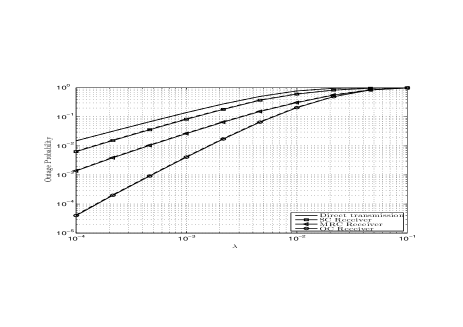
Figure 1: Outage probability versus $\lambda$ for different combining receivers with random relay selection. Simulation results are shown with dashed lines.

where

$${P}_{SC}^{BS}\!=1\!-\mathbb{E}\left\{{\textbf{1}}(x_{k}\rightarrow x_{D}|\Psi\backslash\{x_{\mathbb{R}}\})\right\}.$$ (20)

Note that we obtained a lower bound for ${P}_{SC}^{BS}$ in (27) which yields a lower bound for the outage probability of the SC receiver at the destination with best relay selection.

III-C2 Random Relay Selection

The outage probability of random relay selection follows from (19) by replacing $P_{SC}^{BS}$ with $P_{SC}^{RS}$ , given in (13).

IV Numerical and Simulation Results

In this section, we study the accuracy of the derived analytical results and compare the outage probability of OC, MRC and SC schemes with best and random relay selection. In all simulations, we have set $\alpha=4$, $\beta=3$ dB, $d=10$ m, $d_{s}=7$ m and $\phi=\frac{\pi}{3}$, unless stated otherwise. To ensure a fair comparison, the SIR threshold of cooperative transmission is set to be twice as much as direct transmission threshold. This is because, in the broadcasting phase, the source uses half of the channel uses and in the relaying phase, the relay uses the remaining channel uses.

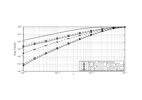
Figure 2: Outage probability versus $\lambda$ for different combining receivers with best relay selection .

The performance of OC and sub-optimal combining schemes (MRC and SC) can be further ascertained by referring to Fig. 1, where the probability of outage as a function of node density, $\lambda$ is shown for random relay selection. Analytical expressions in (12), (17), and  (20) are confirmed as they are seen to follow the simulations tightly. The performance improvement of all three combining schemes compared to the direct transmission is noticeable for all intensities. Note that although increasing the intensity of nodes results in increasing the number of qualified relay nodes, the interference caused by these relay nodes in relaying phase is increased. Hence, for higher values of intensity the performance of all schemes are converging to the same values.

The effect of best relay selection on the outage performance of combining schemes is investigated in Fig. 2 and the tightness of proposed lower bound for OC and SC receiver are validated. Comparing Fig. 1 and Fig 2 reveals that best relay selection significantly outperforms the random relay selection as expected.

Our observation of the relation between the outage performance of combining schemes and selection region parameters which due to the space limitation are not shown in simulations, reveals that: 1) There is an optimal value of the parameter $\phi$ for each combining scheme that achieves the maximum success probability. 2) Increasing the parameter $\phi$ beyond its optimum value does not degrade the success probability. The reason is that although enlarging the selection region increases the possibility of being relay nodes in this area and consequently increases the intensity of interferer set for the second hop, the relay selection strategy only selects a single relay, and thus the intensity of the interferers for the second hop is upper bounded. Therefore, the success probability remains constant.

V Conclusion

The performance of relay selection schemes along with different combining schemes for cooperative transmissions in ad hoc networks have been studied. In particular, we have obtained closed-form expressions for the outage probability of OC, MRC, and SC receivers at the destination with random relay selection. We have also derived two useful tight lower bounds for the OC and SC receivers with best relay selection. The accuracy of the analytical results has been validated using Monte Carlo simulations.

Appendix A Proof of Proposition 1

The proof of Proposition 2 is accomplished in four steps as follows:
Step 1: The outage probability corresponding to the event $\mathcal{O}\left(g_{SD}/I_{\Phi^{t}_{D}},\beta\right)$ is given by (6).
Step 2: The outage event $\mathcal{O}\left(g_{S\mathbb{R}}/I_{\Phi^{t}_{\mathbb{R}}},\beta\right)$ is equivalent to the event that the potential relay set $\Phi^{r}_{o}$ is empty. Note that $\Phi^{r}_{o}$ which is derived by thinning the PPP $\Phi^{r}$, is still a PPP and Marking theorem of Poisson processes [15] gives its density as

$$\Lambda_{o}(x) =(1-p)\lambda\mathbb{E}\left\{\textbf{1}(x_{S}\rightarrow x_{k}|\Phi^{t}\backslash\{x_{S}\})\right\}$$

$$=(1-p)\lambda\exp\left(-\eta\beta^{\delta}\ r^{2}\right).$$ (21)

Therefore, the outage probability corresponding to desired outage event is given by

$$P_{r}=\exp(-\mu_{o}(\mathcal{A})),$$ (22)

where $\mu_{o}(\mathcal{A})$ denotes the mean measure of $\Phi^{r}_{o}$ and

$$\mu_{o}(\mathcal{A})=\int_{\mathcal{\mathcal{A}}}\Lambda_{o}(dx),$$ (23)

in which $\mathcal{A}$ is the selection region and $dx$ denotes a two-dimensional variable of integration over the polar area. Finally, by substituting (21) into (23) the outage probability in (22) is obtained for sectorized selection region as

$$P_{r}=\exp\left(-\frac{\phi(1-p)\lambda}{\beta^{\delta}\eta}\gamma\left(1,\eta\beta^{\delta}d_{s}^{2}\right)\right).$$ (24)

Step 3: The outage probability corresponding to the outage event $\mathcal{O}\left(SIR_{OC},\beta\right)$ can be written as

$${P}_{OC}^{BS}\! =\textnormal{Pr}\left(SIR_{SD}+SIR_{\mathbb{R}D}<\beta\right)$$

$$=\!\int_{0}^{\beta}\!F_{\mathbb{R}D}(\beta\!-\!y)f_{{SD}}(y)dy,$$ (25)

where $F(\cdot)$ and $f(\cdot)$ denotes cdf and probability density function (pdf) of the RV, respectively. $f_{SD}(y)$ can be found simply by taking the first order derivation of (6), which yields

$$f_{SD}(y)=\eta d^{2}\delta y^{\delta-1}\exp(-\eta d^{2}y^{\delta}).$$ (26)

A lower bound for $F_{\mathbb{R}D}(\beta)$ is obtained as

$$F_{\mathbb{R}D}(\beta)=1-\mathbb{E}\left\{{\textbf{1}}(x_{k}\rightarrow x_{D}|\Psi\backslash\{x_{\mathbb{R}}\})\!\right\}$$

$$~{}\!=\!1\!-\!\textnormal{Pr}\left(\max_{x_{k}\in\Phi^{r}_{o}}\left\{h_{kD}\ell(x_{k}-x_{D})\right\}>\beta I_{\Psi}\right)$$

$$~{}\!=\!1\!-\!\mathbb{E}\left\{\prod_{x_{k}\in\Phi^{r}_{o}}\exp\left(-\frac{\beta I_{\Psi}}{\ell(x_{k}-x_{D})}\right)\right\}$$

$$~{}\!\stackrel{{\scriptstyle(a)}}{{=}}\!1\!-\!\mathbb{E}\left\{\exp\!\left(\!-\!\int_{\mathcal{A}}\!{\!\left[1\!-\!\exp\!\left(\!-\!\frac{\beta I_{\Psi}}{\ell(x_{k}\!-\!x_{D})}\right)\!\right]\Lambda_{o}(dx)}\!\right)\!\right\}$$

$$~{}\!\stackrel{{\scriptstyle(b)}}{{\geq}}\!1\!-\!\exp\left(-\int_{\mathcal{A}}\!{\!\left[1\!-\!\mathbb{E}\left\{\exp\left(-\frac{\beta I_{\Psi}}{\ell(x_{k}\!-\!x_{D})}\right)\right\}\right]\Lambda_{o}(dx)}\right)$$

$$~{}\!\stackrel{{\scriptstyle(c)}}{{=}}\!1\!-\!\exp\left(-\int_{\mathcal{A}}\!{\left[1-\exp(-\eta_{I}\beta^{\delta}d_{\mathbb{R}D}^{2})\right]\Lambda_{o}(dx)}\right),$$ (27)

where (a) follows from the generating functional of the PPP, $\Phi^{r}_{o}$ with intensity $\Lambda_{o}(x)$ and (b) follows by using the the Jensen’s inequality. (c) holds by taking the expectation over $I_{\Psi}$ where the exponential distribution of channel gains and the generating functional of $\Psi$ have been used. Moreover, $\eta_{I}=c\Lambda_{I}$ where $\Lambda_{I}$ is the intensity of interferers for second hop transmission. The details of intensity evaluation for the second hops’ interferers are deferred to Appendix B. Plugging (27) together with (26) into (25), yields the lower bound on $P_{OC}^{BS}$ in (25).

Step 4: Referring to the outage event in (8), the overall outage probability of the cooperative transmission with OC receiver and best relay selection is given by

$$P_{out}^{OC,BS}=P_{d}\left(\left(1-P_{r}\right)\left(1-P_{OC}^{BS}\right)+P_{OC}^{BS}\right)$$ (28)

Plugging (6), (24) and (25) into (28) and after some manipulations gives the desired result in (11).

Appendix B Intensity of the Interferer set

Deriving the intensity of interferer set for the second-hop transmission is equivalent to exploit how many selected relays are there for transmission in the second hop. Provided that the potential relay set is not empty, since each source only selects a single relay in both best relay selection and random relay selection, it is clear that the intensity of interferer set is at most $p\lambda$, which is the intensity of the source nodes. Let us denote the probability that an arbitrary source node successfully selects one relay node by $q$. Then, the intensity of active relay nodes in second stage of cooperative transmission protocol is $pq\lambda$, which is also the intensity of the interferers. Note that $q$ is proportional to the probability that at least there is one relay in potential relay set which for a typical pair is mathematically described by

$$q=1-P_{r}=1-\exp(-\mu_{o}(\mathcal{A})).$$ (29)

Therefore, in the case of a sectorized selection region, the intensity of interferer set in second stage of transmission, $\Lambda_{I}$, is given by

$$\Lambda_{I} =p\lambda\left(1-\exp\left(-(1-p)\lambda\int_{\mathcal{A}}{\exp\left(-\eta\beta^{\delta}\ r^{2}\right)dx}\right)\right)$$

$$=p\lambda\gamma\left(1,\frac{\phi(1-p)\lambda}{\eta\beta^{\delta}}\gamma\left(1,\eta\beta^{\delta}d_{s}^{2}\right)\right).$$ (30)

$${P}_{MRC}^{RS} =1-\mathbb{E}\left\{\frac{1}{\mu_{1}-\mu_{2}}\left[\mu_{1}\exp\left(-\mu_{2}\beta\left(\frac{u}{u+v}I_{\Phi^{t}_{D}}+\frac{v}{u+v}I_{\Psi}\right)\right)-\right.\right.$$

$$\qquad\qquad\qquad\qquad\qquad\left.\left.\mu_{2}\exp\left(-\mu_{1}\beta\left(\frac{u}{u+v}I_{\Phi^{t}_{D}}+\frac{v}{u+v}I_{\Psi}\right)\right)\right]\right\}$$

$$\stackrel{{\scriptstyle(a)}}{{=}}\!1\!-\!\mathbb{E}\left\{\frac{1}{\mu_{1}\!-\!\mu_{2}}\!\left[\mu_{1}\!\!\prod_{x_{k}\in\Phi^{t}\backslash\{x_{S}\}}\!\!\!\!\mathcal{M}_{W_{1}}\!\left(\mu_{2}\beta\ell(x_{k}-x_{D})\right)\!\!\prod_{y_{k}\in\Psi\backslash\{\mathbb{R}\}}\!\!\!\!\mathcal{M}_{W_{2}}\!\!\left(\mu_{2}\beta\ell(y_{k}-x_{D})\right)\!-\right.\right.$$

$$\qquad\qquad\qquad\qquad\left.\left.\mu_{2}\!\!\prod_{x_{k}\in\Phi^{t}\backslash\{x_{S}\}}\!\!\!\!\mathcal{M}_{W_{1}}\!\!\left(\mu_{1}\beta\ell(x_{k}-x_{D})\right)\!\!\prod_{y_{k}\in\Psi\backslash\{\mathbb{R}\}}\!\!\!\mathcal{M}_{W_{2}}\!\!\left(\mu_{1}\beta\ell(y_{k}-x_{D})\right)\!\right]\!\right\}$$ (36)

Appendix C Proof of Proposition 3

Before deriving the outage probability we will need the following lemma.

Lemma 1

Given three RVs $u\sim\mathcal{E}(\mu_{1})$, $v\sim\mathcal{E}(\mu_{2})$, and $z\sim\mathcal{E}(1)$, the moment generating function (MGF) of $W_{1}=uz/(u+v)$, $\mathcal{M}_{W_{1}}(s)=\mathbb{E}\{\exp(-sW_{1})\}$ is given by

$$\mathcal{M}_{W_{1}}(s) \!=\!1-\!\frac{s}{s+1}\times$$

$$\quad\quad\left[\!1\!-\!\frac{\mu_{1}}{\mu_{2}}\frac{1}{s\!+1}G_{22}^{22}\left(\frac{\mu_{1}}{\mu_{2}}\frac{1}{s+\!1}\ \Bigg{|}\ {\!\!\!-1,0\atop 0,0}\right)\right],$$ (31)

where $G_{pq}^{mn}\left(s\ |\ {a_{1}\cdots a_{p}\atop b_{1}\cdots b_{q}}\right)$ denotes the Meijer’s G-function defined in [11, Eq. (9.301)]. With appropriate changes of the mean indices in (31), the MGF of $W_{2}=vz/(u+v)$, can be expressed as

$$\mathcal{M}_{W_{2}}(s) \!=\!1-\!\frac{s}{s+1}\times$$

$$\quad\quad\left[\!1\!-\!\frac{\mu_{2}}{\mu_{1}}\frac{1}{s\!+1}G_{22}^{22}\left(\frac{\mu_{2}}{\mu_{1}}\frac{1}{s+\!1}\ \Bigg{|}\ {\!\!\!-1,0\atop 0,0}\right)\right],$$ (32)

Proof:

See Appendix D ∎

Following similar steps as in the OC case with random relay selection, we get the outage probability as (16).

What remains to calculate is then to determine the outage probability ${P}_{MRC}^{RS}$. Let us define

$$u\triangleq g_{SD},\quad v\triangleq g_{\mathbb{R}D}.$$ (33)

The RVs, $u$ and $v$ are exponentially distributed with parameter $\mu_{1}=d^{\alpha}$ and $\mu_{2}=d_{\mathbb{R}D}^{\alpha}$, respectively. We recall that for random relay selection case, the RV $g_{\mathbb{R}D}$ is considered as an arbitrary exponential RV. It can be shown that the SIR in (14) is of the form of [17, Eq. (28)], i.e.,

$$SIR_{MRC} =\frac{|\bm{c}_{s}|^{2}}{\sum_{i=1}^{L}|\bm{\nu}_{i}|^{2}},$$ (34)

where $|\bm{c}_{s}|^{2}=u+v$, $\bm{\nu}_{i}=\bm{c}_{s}^{\dagger}\bm{c}_{i}/|\bm{c}_{s}|$, and $L=|\Phi^{t}|+|\Psi|$ with $\bm{c}_{i}$ being the channel coefficient between the interferer $i$ and destination and $|\cdot|$ being the cardinality of a set. Therefore, it can be shown that $\bm{\nu}_{i}$’s are independent of $\bm{c}_{s}$ [17] and thus ${P}_{MRC}^{RS}$ can be written as

$${P}_{MRC}^{RS} =\textnormal{Pr}\left((u+v)<\beta\left[\frac{u}{u+v}I_{\Phi^{t}_{D}}+\frac{v}{u+v}I_{\Psi}\right]\right).$$ (35)

Using the cdf of $u+v$ given in [1, Eq. (40)], the outage probability can be expressed as (36) at the top of this page, where ($a$) follows by taking the expectation with respect to $W_{1}$ and $W_{2}$. Using Lemma 1, the generating functional of Poisson processes, $\Phi^{t}$ and $\Psi$, and [11, Eq. (3.194.4) and Eq. (7.811.2)] gives, after some manipulation, the desired result in (17).

Appendix D Proof of Lemma 1

In order to obtain the MGF of $W_{1}$, we first derive the cdf of $W_{1}$ as

$$F_{W_{1}}(w) \!=\!\int_{0}^{\infty}\textnormal{Pr}\left(z<w\left(1+\gamma\right)\right)f_{\Upsilon}(\gamma)d\gamma,$$ (37)

where $\gamma\triangleq\frac{u}{v}$, and its pdf can be readily obtained as

$$f_{\Upsilon}(\gamma)=\frac{\frac{\mu_{1}}{\mu_{2}}}{(\gamma+\frac{\mu_{1}}{\mu_{2}})^{2}}.$$ (38)

Plugging (38) into (37), using [18, Eq. (5.1.4) and Eq. (13.6.30)], and after some manipulations, we get the cdf in closed-form as

$$F_{W_{1}}(w) \!=1\!-\!\exp(-w)\left[1-\frac{\mu_{1}}{\mu_{2}}w\Psi\left(1,1,\frac{\mu_{1}}{\mu_{2}}w\right)\right],$$ (39)

where $\Psi(\cdot,\cdot,\cdot)$ denotes the Tricomi confluent hypergeometric function [11, Eq. (9.211.4)]. Now, the MGF of $W_{1}$ can be directly found from

$$\mathcal{M}_{W_{1}}(s) =s\mathcal{L}(F_{W_{1}}(w))-F_{W_{1}}(0),$$

where $\mathcal{L}(\cdot)$ denotes the Laplace transform and $F_{W_{1}}(0)=0$. Using [19, Eq. (3.36.1.7)] one can obtain the MGF of $W_{1}$ in closed-form as (31) and the lemma is proved.

References

- [1] J. Laneman, D. Tse, and G. Wornell, “Cooperative diversity in wireless networks: Efficient protocols and outage behavior,” IEEE Trans. Inf. Theory, vol. 50, pp. 3062–3080, Dec. 2004.
- [2] A. Bletsas, A. Khisti, D. P. Reed, and A. Lippman, “A simple cooperative diversity method based on network path selection,” IEEE J. Sel. Areas Commun., vol. 24, pp. 659–672, Mar. 2006.
- [3] M. Kountouris and J. Andrews, “Throughput scaling laws for wireless ad hoc networks with relay selection,” in Proc. IEEE VTC Spring 2009, Barcelona, Spain, April 2009, pp. 1 – 5.
- [4] H. Wang, S. Ma, T.-S. Ng, and H. V. Poor, “A general analytical approach for opportunistic cooperative systems with spatially random relays,” IEEE Trans. Wireless Commun., vol. 10, pp. 4122–4129, Dec. 2011.
- [5] R. K. Ganti and M. Haenggi, “Analysis of uncoordinated opportunistic two-hop wireless ad hoc systems,” in Proc. IEEE ISIT 2009, Seoul, South Korea, July 2009, pp. 1020 – 1024.
- [6] S.-R. Cho, W. Choi, and K. Huang, “Qos provisioning relay selection in random relay networks,” IEEE Trans. Veh. Technol., vol. 60, pp. 2680 – 2689, July 2011.
- [7] S. Weber, J. G. Andrews, and N. Jindal, “An overview of the transmission capacity of wireless networks,” IEEE Trans. Commun., vol. 58, pp. 3593–3604, Dec. 2010.
- [8] D. Li, C. Yin, and C. Chen, “A selection region based routing protocol for random mobile ad hoc networks with directional antennas,” in Proc. IEEE GLOBECOM 2010, Miami, FL., Dec. 2010, pp. 1–5.
- [9] M. K. Simon and M. S. Alouini, Digital Communication over Fading Channels, 2nd ed. New York, NY: John Wiley & Sons, Inc., 2005.
- [10] F. Baccelli, B. Blaszczyszyn, and P. Mühlethaler, “An Aloha protocol for multihop mobile wireless networks,” IEEE Trans. Inf. Theory, vol. 52, pp. 421–436, Feb. 2006.
- [11] I. S. Gradshteyn and I. M. Ryzhik, Table of Integrals, Series and Products, 7th ed. Academic Press, 2007.
- [12] A. Bletsas, A. G. Dimitriou, and J. N. Sahalos, “Interference-limited opportunistic relaying with reactive sensing,” IEEE Trans. Wireless Commun., vol. 9, pp. 14–20, Jan. 2010.
- [13] O. B. S. Ali, C. Cardinal, and F. Gagnon, “Performance of optimum combining in a poisson field of interferers and rayleigh fading channels,” IEEE Trans. Wireless Commun., vol. 9, pp. 2461–2467, Aug. 2010.
- [14] E. G. Larsson and Y. Cao, “Collaborative transmit diversity with adaptive radio resource and power allocation,” IEEE Commun. Lett., vol. 9, pp. 511–513, June 2005.
- [15] D. Stoyan, W. Kendall, and J. Mecke, Stochastic Geometry and its Applications, 2nd ed. John Wiley and Sons, 1996.
- [16] Z. Gong and M. Haenggi, “Interference and outage in mobile random networks: Expectation, distribution, and correlation,” IEEE Trans. Mobile Comput., 2012, submitted. Available at http://www.nd.edu/~mhaenggi/pubs/tmc12b.pdf.
- [17] A. Shah and A. M. Haimovich, “Performance analysis of maximal ratio combining and comparison with optimum combing for mobile radio communications with cochannel interferece,” IEEE Trans. Veh. Technol., vol. 49, pp. 1454 – 1463, July 2000.
- [18] M. Abramowitz and I. A. Stegun, Handbook of Mathematical Functions With Formulas, Graphs, and Mathematical Tables., 9th ed. New York: Dover, 1970.
- [19] A. P. Prudnikov, Y. A. Brychkov, and O. I. Marichev, Integral and Series , vol. 4: Direct Laplace Transforms. Gordon and Breach, New York-London, 1992.