Measuring ultrasmall time delays of light by joint weak measurements

Abstract

We propose to use weak measurements away from the weak-value amplification regime to carry out precision measurements of time delays of light. Our scheme is robust to several sources of noise that are shown to only limit the relative precision of the measurement. Thus, they do not set a limit on the smallest measurable phase shift contrary to standard interferometry and weak-value based measurement techniques. Our idea is not restricted to phase-shift measurements and could be used to measure other small effects using a similar protocol.

Twenty years after the proposal Aharonov1988 of Aharonov, Albert, and Vaidman, several experiments have demonstrated the possibility to measure tiny physical effects using the so-called weak-value amplification scheme Hosten2008 ; Dixon2009 ; Gorodetski2012 . These ideas have paved the way for new approaches to precision measurements in general, and have triggered a great deal of further theoretical and experimental developments.

Recently, Hosten and Kwiat Hosten2008 were able to experimentally confirm the spin Hall effect of light by measuring a polarization-dependent displacement of a laser beam to a precision of 1 ​Å using weak-value amplification. Gorodetski et al. Gorodetski2012 investigated the plasmonic spin Hall effect. Dixon et al. Dixon2009 determined the angle of a mirror to a precision of the order of 500 frad by measuring deflection of light off the mirror. Several experiments were proposed in order to enhance the precision of the measurement of longitudinal phase shifts of light Brunner2010 , or amplify the single-photon nonlinearity to a measurable effect Feizpour2011 . An application to charge sensing in a solid-state context has also been put forward Zilberberg2011 . The advantages of weak-value amplification schemes for suppressing technical noise were investigated in Feizpour2011 ; Starling2009 ; Nishizawa2012 , and Kedem2012 showed how technical noise could even improve the precision in this scheme. Ways to optimize the initial meter wavefunction were studied in Susa2012 .

There was a number of attempts to go beyond the weak-value formalism. This includes, for instance, higher-order expansions for nearly orthogonal pre- and post-selected states Geszti2010 ; Wu2011 ; Nakamura2012 ; Pang2012 ; Kofman2012 , or the use of full counting statistics DiLorenzo2012 , and orbital-angular-momentum pointer states Puentes2012 . The effect of decoherence was investigated in Ref. Knee2013 . The limits of amplification for arbitrary coupling strength were addressed in Koike2011 ; Zhu2011 . Connections of the weak-value formalism with the theoretical tools of precision metrology were made in Hofmann2011 ; Hofmann2012 . Weak values were also related to quasiprobability distributions of incompatible observables Bednorz2012 .

In this Letter, we would like to propose a scheme to measure very small time delays, or longitudinal phase shifts. The idea is to use weak measurements away from the weak-value amplification regime and to exploit the full information contained in the correlations induced by the time delay between frequency and polarization of photons going through the interferometer. This procedure is not limited to time-delay measurements and could be used for other precision measurements. For example, it is readily applicable to measurements of ultrasmall beam deflections by slightly modifying the protocol of Dixon et al. Dixon2009 . The idea of carrying out a full joint measurement of two weakly entangled degrees of freedom could be relevant in many domains such as charge sensing in solid state physics Zilberberg2011 , precision metrology, and gravitational wave detection.

Following Ref. Brunner2010, we are interested in measuring with high precision a small interaction parameter $\tau$ which couples two physical systems. We will call them system and meter as is customary in weak-value protocols, and the effect of the coupling is described by an unitary operator

$$\hat{U}=e^{i\tau\hat{A}\hat{x}}\,,$$ (1)

where $\hat{A}$ is an operator acting on the system and $\hat{x}$ acts on the meter. There are many different situations where the measurement of a small coupling constant $\tau$ is potentially relevant. For example the interaction can be an interesting but very small physical effect, like the spin Hall effect of light Hosten2008 ; or $\tau$ can be a quantity of direct interest, describing the angle of a mirror, see Dixon2009 , or describing the amplitude of a gravitational wave in an interferometric setup. In this Letter we will consider a setup where a time delay in an optical interferometer plays the role of the interaction parameter $\tau$, as in Brunner2010 .

The interaction (1) with small $\tau$ is formally similar to a weak measurement of the observable $\hat{A}$ of the system. Therefore by adding a pre- and post-selection of the system in states $\left|i\right\rangle$ and $\left|f\right\rangle$ respectively, see Aharonov1988 , we obtain the weak value of the observable $\hat{A}$, $A_{w}=\left\langle f\right|\hat{A}\left|i\right\rangle/\left\langle f|i\right\rangle$ in the meter averages $\langle\hat{p}\rangle=\tau\text{Re}A_{w}$, and $\langle\hat{x}\rangle=-2\tau\left\langle\psi\right|\hat{x}^{2}\left|\psi\right\rangle\text{Im}A_{w}$, where $\left|\psi\right\rangle$ is the initial state of the meter. Those results are only valid up to linear order in $\tau$, which is enough for our purposes, but the meter averages can also be expressed exactly using a generalized form of weak values Dressel2012 . Weak-value amplification is based on the fact that it is possible to obtain arbitrarily large weak values by choosing almost orthogonal initial and final states, $\left\langle f|i\right\rangle\rightarrow 0$, thereby amplifying the small interaction parameter $\tau$. The price to pay for obtaining large weak values is the small probability $P_{\text{ps}}=\left|\left\langle f|i\right\rangle\right|^{2}$ of a successful post-selection. Weak-value amplification does not increase the statistical information because the amplification of the signal is exactly counterbalanced by the small success rate of the post-selection. However the amplification allows to overcome technical limitations, e.g. detector resolution or readout noise. On the other hand, stringent post-selections lead to an increased sensitivity against certain types of noise. For instance background noise, e.g. stray photons hitting the detector in optics experiments, is a limiting factor of how small the post-selection can be since the rate of useful, post-selected, photons must be significantly larger than the background. Another critical type of noise is due to errors in the post-selection itself.

Conceptually, as is the case for all quantum mechanical measurements Dressel2010 , the crucial information in imaginary weak-value amplification is not the average shift of the meter, but the correlations induced by the interaction between the system and the meter. These are generally probed by joint measurements on the meter and system. Weak-value amplification constitutes a partial joint weak measurement, since measurement outcomes are retained only if the system is found in a certain state. Remarkably, it turns out that all the useful correlations for the estimation of $\tau$ are contained in the small post-selection regime. However, additional information on other aspects of the experiment is included in the other outcomes. In the presence of noise, this additional information turns out to be useful to precisely evaluate $\tau$. In the following, we will present an example where carrying out a full joint weak measurement outperforms weak-value amplification.

Time-delay measurements.– We consider a Mach-Zehnder interferometer for laser light, see Fig. 1a. Encoding the which-path information in a two-level system allows us to write the effect of the time delay as

$$U=e^{i\tau\hat{\sigma}_{y}\hat{H}/2}\,,$$ (2)

where $\hat{\sigma}_{y}$ acts on the which-path space, and $\hat{H}$ is the Hamiltonian of the laser light. The time delay now takes the role of the interaction parameter in Eq. (1), and the photon frequencies (which are contained in $\hat{H}$) the role of the pointer variable $x$. The incoming light is evenly split into the two arms with opposite circular polarizations by a polarizing beam splitter. The two arms then recombine at another polarizing beam splitter with linearly polarized outputs. The direction of the linear polarization is described by the azimuthal angle $\phi$ on the Poincaré sphere. The two output ports $q=\pm 1$ are monitored by spectrometers. In the weak-value language, the pre-selected polarization state is $\left|i\right\rangle=(\left|-\right\rangle+\left|+\right\rangle)/\sqrt{2}$ and the two post-selected states at detector $q$ are $\left|f_{q}\right\rangle=(\left|-\right\rangle+qe^{i\phi}\left|+\right\rangle)/\sqrt{2}$. We are interested in ultrasmall time delays with $\omega_{\text{max}}\tau\ll 1$, where $\omega_{\text{max}}$ is the maximal frequency contained in the laser light.

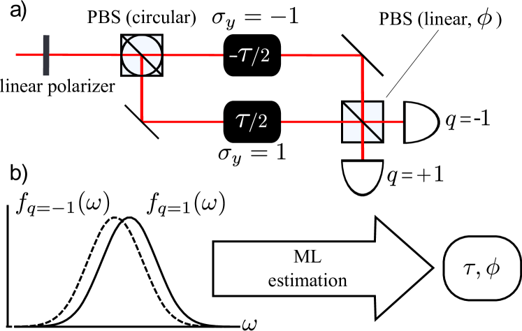
Figure 1: (a) Mach-Zehnder interferometer for laser light with a time-delay asymmetry $\tau$. The incoming beam is linearly polarized and then evenly split by a polarizing beam splitter (PBS) into the two arms with opposite circular polarizations, $\sigma_{y}=\pm 1$. The beams are recombined at a second PBS with linearly polarized outputs. The direction of the linear polarization is described by the azimuthal angle $\phi$ on the Poincaré sphere. Two spectrometers labeled by $q=\pm 1$ measure the spectrum of the outgoing light. (b) Graphical representation of the estimation process. The values of $\tau$ and $\phi$ are extracted from the spectra measured by the two detectors by a maximum-likelihood (ML) estimation technique as described in the text.

A laser pulse with normalized spectrum $p_{0}(\omega)$, which can be interpreted as a probability density, is sent through the interferometer. The probability density of outcomes is then given by

$$p_{q}(\omega;\tau,\phi)=\frac{1}{2}p_{0}(\omega)[1+q\exp(-\epsilon^{2}/2)\cos(\phi-\omega\tau)]\,,$$ (3)

where we have introduced Gaussian fluctuations of amplitude $\epsilon$ of the alignment parameter $\phi$, i.e., convoluted the bare probability density with a fluctuation kernel

$$\xi(\phi,\phi^{\prime})=\frac{1}{\sqrt{2\pi}\epsilon}\exp\left(-\frac{(\phi-\phi^{\prime})^{2}}{2\epsilon^{2}}\right)$$ (4)

that describes fluctuations around the average alignment $\phi$. Note that only the fluctuations with a correlation time smaller than the measurement duration are included in $\epsilon$. Fluctuations with a longer correlation time will modify the effective value of $\phi$. From now on we make the realistic assumption $\epsilon\ll 1$. It can be shown that fluctuations of the alignment of the circular polarizing beam splitter and of the linear polarizer can also be encompassed in $\epsilon$.

Our goal is to find an estimate of the values of the parameters $\tau,\phi$ from outcomes of an experiment following the probability distribution (3). Although $\phi$ is in principle controlled experimentally, its estimation permits to remove possible systematic errors. The quantity produced by the experiment is a set of observed frequencies $f_{q}(\omega)$, which, in principle, converge to $p_{q}(\omega;\tau,\phi)$ as the number $N$ of measured photons is increased.

We use the maximum likelihood procedure Helstrom1976 to provide unbiased estimates of the values of the parameters, see Fig. 1b. This is achieved by maximizing the log-likelihood function $l(\tau,\phi)$ defined as

$$l(\tau,\phi)=\sum_{q=\pm 1}\int d\omega\;f_{q}(\omega)\log p_{q}(\omega;\tau,\phi)\,.$$ (5)

Maximizing the log-likelihood yields two equations which have to be solved numerically in the general case. However, for the special case of almost equal intensities at the two detectors, $|\phi-\omega\tau-\frac{\pi}{2}|\ll 1$, analytical expressions can be derived

$$\phi =\frac{\pi}{2}-\exp(\epsilon^{2}/2)\sum_{q}qP_{q}\,,$$ (6)

$$\tau =\frac{1}{4\Delta\omega}\exp(\epsilon^{2}/2)\left(\frac{1}{\Delta\omega}\sum_{q}qP_{q}\langle\omega\rangle_{q}-\sum_{q}qP_{q}\right)\,,$$ (7)

where $P_{q}$ is the integrated fraction of outcomes in detector $q$, and $\langle\cdot\rangle_{q}$ denotes the average value in detector $q$. The frequency spread $\Delta\omega$ of the initial distribution is given by $(\Delta\omega)^{2}=\sum_{q}P_{q}\langle\omega^{2}\rangle_{q}-\left(\sum_{q}P_{q}\langle\omega\rangle_{q}\right)^{2}$. The estimates (6,7) depend on measurement results and on one unknown amplitude $\epsilon$ that characterizes alignment fluctuations. Remarkably, $\exp(\epsilon^{2}/2)$ only appears as an overall multiplicative factor. Thus, the ultimate error $\Delta\tau_{\text{ult}}$ on the estimation of $\tau$ by assuming $\epsilon=0$ (since its value is unknown, yet realistically $\epsilon\ll 1$) scales with $\tau$, i.e. only a relative error occurs that does not limit the smallest $\tau$ that can be measured. Equation (7) is one of the main results of our Letter.

Aside from the errors due to technical noise, statistical uncertainties also contribute to the estimation error. For a finite number $N$ of detected photons, the statistical errors are provided by the Cramér-Rao bound Helstrom1976 : $\Delta\tau_{\text{stat}}\geq\sqrt{(\mathcal{I}^{-1})_{\tau\tau}/N}$, and $\Delta\phi_{\text{stat}}\geq\sqrt{(\mathcal{I}^{-1})_{\phi\phi}/N}$, where $\mathcal{I}$ is the Fisher information matrix given by

$$\mathcal{I}_{yz}=\sum_{q=\pm 1}\int dx\;p_{q}(x;\tau,\phi)\left(\partial_{y}\log p_{q}\right)\left(\partial_{z}\log p_{q}\right)\,.$$ (8)

As a side remark, note that the logarithmic derivative $\partial_{\tau}\log p_{q}$ is connected to the weak value of $\sigma_{y}$ in detector $q$, see Ref. Hofmann2012, for a discussion. Asymptotically, i.e., for large $N$, the Cramér-Rao bounds are saturated by the maximum-likelihood procedure. In the case of almost equal intensities at the two detectors we obtain

$$\Delta\tau_{\text{stat}}\geq\frac{\exp(\epsilon^{2}/2)}{4\Delta\omega\sqrt{N}}\,,$$ (9)

which shows that the fluctuations of $\phi$ do not increase significantly statistical noise. The number of detected photons $N$ required to obtain a good estimate of $\tau$ is of the order $10/(\Delta\omega\tau)^{2}$. Estimating a time delay of the order of $1$ attosecond with ultrashort laser pulses with $\Delta\omega\approx 10^{15}\text{Hz}$ would require detecting $10^{7}$ photons. A typical pulse contains typically $10^{13}$ photons which would be enough to measure time delays of the order of $1$ zeptosecond corresponding to a displacement of 100fm.

Split detectors.– We would now like to apply this result to an actual detector with a finite resolution. This will in particular shed light on the roles played by the resolution and readout noise of the detector. In principle, the results of the previous section could require measuring the full distribution of $\omega$ without any readout noise. To show that this is not the case we consider “split” detectors which can only discriminate two spectral regions $\omega>\omega_{0}$, leading to a measurement result $r=+1$, and $\omega<\omega_{0}$, leading to $r=-1$. We also add readout noise from the outset. We will see that our conclusion from Eq. (7) (viz. that there is no absolute lower limit on the smallest value of $\tau$ that can be measured) survives even in this extreme case.

To make up for losing the detector resolution some a priori knowledge of the initial frequency distribution $p_{0}(\omega)$ is required. For analytical calculations we will assume an initial Gaussian distribution, but the results will depend only quantitatively on the shape. In practice the distribution should be measured and the calculations done numerically. We thus assume $p_{0}(\omega)\approx e^{-(\omega-\omega_{0})^{2}/2(\Delta\omega)^{2}}/\sqrt{2\pi}\Delta\omega$ where the tails should, in principle, be truncated since $0\leq\omega\leq\omega_{\text{max}}$. The probabilities of the two possible outcomes $r=\pm 1$ at the two detectors $q=\pm 1$ at second order in the small quantity $\Delta\omega\tau$ read

$$p_{rq}=\frac{1}{4}[1+q\exp(-\epsilon^{2}/2)(1-\frac{1}{2}(\Delta\omega\tau)^{2})\cos\phi]$$

$$+rq\exp(-\epsilon^{2}/2)\frac{\Delta\omega\tau}{2\sqrt{2\pi(1+(\Omega/\Delta\omega)^{2})}}\sin\phi\,,$$ (10)

where we allowed for a frequency detection uncertainty of order $\Omega$ modeled as Gaussian white noise.

Denoting the measured probabilities by $f_{rq}$, the maximum likelihood estimation can be analytically carried out in the regime $|\sin\phi|\gg\Delta\omega\tau$, and yields $\cos\phi=\exp(\epsilon^{2}/2)(P_{+}-P_{-})$ in terms of the integrated fraction of outcomes $P_{q}=\sum_{r}f_{rq}$, and

$$\tau=\frac{\sqrt{2\pi(1+(\Omega/\Delta\omega)^{2})}}{8\Delta\omega\sqrt{\exp(-\epsilon^{2})-(P_{+}-P_{-})^{2}}}\sum_{r,q}\frac{rqf_{rq}}{1+q(P_{+}-P_{-})}\,.$$ (11)

The first terms in the expansion of $\tau$ in the fluctuations $\epsilon$ and detection noise $\Omega$ can now be calculated, and we finally obtain

$$\tau=\tau_{0}\left[1+\frac{1}{2}\left(\frac{\epsilon}{\sin\phi}\right)^{2}+\frac{1}{2}\left(\frac{\Omega}{\Delta\omega}\right)^{2}\right]\,,$$ (12)

where $\tau_{0}$ is the estimated value of $\tau$ in the absence of noise, see Eq. (11) with $\epsilon$ and $\Omega$ set to zero. Again the noise does not set an absolute limit on the precision of the estimation of $\tau$ but only a relative precision. The frequency spread $\Delta\omega$ reduces the effect of readout noise. Moreover we observe that in order to minimize the effect of fluctuations of $\phi$, we have to work in the regime $\sin\phi\approx 1$ and not in the weak-value amplification regime of $\sin\phi\approx 0$ where the effect of fluctuations increased.

The statistical uncertainty is given by the Fisher information matrix, which is diagonal in this case, through the Cramér-Rao bound

$$\Delta\tau_{\text{stat}}\geq\frac{\sqrt{2\pi}}{4\Delta\omega\sqrt{N}}\left[1+\frac{1}{2}\left(\frac{\epsilon}{\sin\phi}\right)^{2}+\frac{1}{2}\left(\frac{\Omega}{\Delta\omega}\right)^{2}\right]\,.$$ (13)

Hence the considered fluctuations do not jeopardize the estimation of $\tau$ away from the weak-value amplification regime. We also note that using split detectors leads to a modest increase of statistical noise by a factor $\sqrt{2\pi}$ with respect to Eq. (9). Equations (12,13) demonstrate that even for low-resolution detectors our scheme is robust against readout noise and alignment errors.

Comparison to existing schemes.– Standard interferometry compares two probabilities given by the sine and cosine of the total phase shift given by the combination $\phi-\omega\tau$. This leads to two difficulties: first, to estimate $\tau$ precisely, the laser frequency $\omega$ has to be highly stabilized. Secondly, the alignment $\phi$ cannot be separated from the effect of $\tau$, i.e., alignment errors are a limiting factor to the precision achievable having complete statistical information. This ultimate precision, which cannot be increased by acquiring more measured data, is given by $\Delta\tau_{\text{ult}}=\epsilon/\omega$. In the procedure proposed by Brunner and Simon Brunner2010 that uses the imaginary part of the weak value, the first issue is solved since a large frequency spread $\Delta\omega$ is advantageous for the precise evaluation of $\tau$, which is also true in our scheme. However, the second issue is only partially addressed in Brunner2010 : alignments errors are still a limiting factor, $\Delta\tau_{\text{ult}}=C\epsilon$, where the proportionality constant $C\approx 10^{-18}$ s is three orders of magnitude smaller than for standard interferometry.

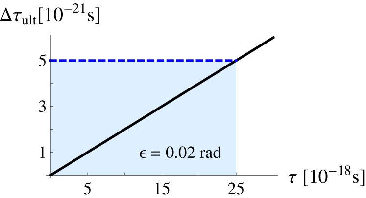
Figure 2: Ultimate precision limit $\Delta\tau_{\text{ult}}$ on the estimation of the physical time delay $\tau$ as a function of $\tau$, in the presence of fluctuations of the alignment $\phi$, see Eq. (4). We assume $\epsilon=0.02$ rad for the plot. The dashed line shows the constant (zeroth-order) contribution of fluctuations to $\Delta\tau_{\text{ult}}=C\epsilon$ for weak-value amplification, here we assume $C\approx 0.25\times 10^{-18}$ s like in Brunner2010 . The solid line is the result of our scheme, $\Delta\tau_{\text{ult}}=\epsilon^{2}\tau/2$. For $\tau<2C/\epsilon$ (shaded area), our scheme outperforms weak-value amplification .

In contrast to that, a major advantage of our scheme is to remove systematic errors as well as fluctuations of the alignment as a limiting factor to the ultimate precision of the time-delay measurement. Alignment fluctuations lead to a relative error $\Delta\tau_{\text{ult}}=\epsilon^{2}\tau/2$ on the estimation of $\tau$, see the discussion after Eq. (7) and the illustration in Fig. 2. This is made possible by working away from the weak-value amplification regime and using all the information contained in the correlations between frequency and polarization of the photons to perform a simultaneous estimation of $\phi$ and $\tau$.

Finally, we would like to mention that if the detector can only measure events at a small rate due to detector saturation, small post-selection probabilities as realized in weak-value amplification schemes permit to effectively increase the rate of measurements Starling2009 . This allows to obtain better statistics, however, if the measurement is limited not by statistics but for other reasons, our method appears preferable.

In conclusion, we have proposed a technique that could be useful to determine very small time delays, or longitudinal phase shifts, due to its robustness with respect to various noise sources. The time delay induces correlations between frequency and polarization of photons going through the interferometer, and our scheme exploits the full information contained in these correlations. The idea is not limited to time-delay measurements and could be used for other precision measurements. In a broader setting, the idea of carrying out a full joint measurement of two weakly entangled degrees of freedom could find applications in many domains such as charge sensing in solid state physics, precision metrology, and gravitational wave detection.

- (1) Y. Aharonov, D. Z. Albert, and L. Vaidman, Phys. Rev. Lett. 60, 1351 (1988).
- (2) O. Hosten and P. Kwiat, Science 319, 787 (2008).
- (3) Y. Gorodetski et al., Phys. Rev. Lett. 109, 013901 (2012).
- (4) P. B. Dixon, D. J. Starling, A. N. Jordan, and J. C. Howell, Phys. Rev. Lett. 102, 173601 (2009).
- (5) N. Brunner and C. Simon, Phys. Rev. Lett. 105, 010405 (2010).
- (6) A. Feizpour, X. Xing, and A. M. Steinberg, Phys. Rev. Lett. 107, 133603 (2011).
- (7) O. Zilberberg, A. Romito, and Y. Gefen, Phys. Rev. Lett. 106, 080405 (2011).
- (8) D. J. Starling, P. B. Dixon, A. N. Jordan, and J. C. Howell, Phys. Rev. A 80, 041803 (2009).
- (9) A. Nishizawa, K. Nakamura, and M.-K. Fujimoto, Phys. Rev. A 85, 062108 (2012).
- (10) Y. Kedem, Phys. Rev. A 85, 060102 (2012).
- (11) Y. Susa, Y. Shikano, and A. Hosoya, Phys. Rev. A 85, 052110 (2012).
- (12) S. Wu and Y. Li, Phys. Rev. A 83, 052106 (2011).
- (13) K. Nakamura, A. Nishizawa, and M.-K. Fujimoto, Phys. Rev. A 85, 012113 (2012).
- (14) T. Geszti, Phys. Rev. A 81, 044102 (2010).
- (15) S. Pang, S. Wu, and Z.-B. Chen, arXiv:1205.0619(2012).
- (16) A. G. Kofman, S. Ashhab, and F. Nori, Phys. Rep. 520, 43 (2012).
- (17) A. Di Lorenzo, Phys. Rev. A 85, 032106 (2012).
- (18) G. Puentes, N. Hermosa, and J. P. Torres, Phys. rev. Lett. 109, 040401 (2012); H. Kobayashi, G. Puentes, and Y. Shikano, Phys. Rev. A 86, 053805 (2012).
- (19) G. C. Knee, G. A. D. Briggs, S. C. Benjamin, E. M. Gauger, Phys. Rev. A 87, 012115 (2013).
- (20) T. Koike and S. Tanaka, Phys. Rev. A 84, 062106 (2011).
- (21) X. Zhu et al., Phys. Rev. A 84, 052111 (2011).
- (22) H. F. Hofmann, M. E. Goggin, M. P. Almeida, and M. Barbieri, Phys. Rev. A 86, 040102(R) (2012).
- (23) H. F. Hofmann, Phys. Rev. A 83, 022106 (2011).
- (24) A. Bednorz and W. Belzig, Phys. Rev. Lett. 105, 106803 (2010).
- (25) J. Dressel and A. N. Jordan, Phys. Rev. Lett. 109, 230402 (2012).
- (26) J. Dressel, S. Agarwal, and A. N. Jordan, Phys. Rev. Lett. 104, 240401 (2010).
- (27) C. W. Helstrom, Quantum detection and estimation theory, Mathematics in Science and Engineering, vol. 123, (Academic Press, New York, 1976).