Superpotentials, quantum parameter space and phase transitions in $\mathcal{N}=1$ supersymmetric gauge theories

Abstract

We study the superpotentials, quantum parameter space and phase transitions that arise in the study of large $N$ dualities between $\mathcal{N}=1$ SUSY $U(N)$ gauge theories and string models on local Calabi-Yau manifolds. The main tool of our analysis is a notion of spectral curve characterized by a set of complex partial ’t Hooft parameters and cuts given by projections on the spectral curve of minimal supersymmetric cycles of the underlying Calabi-Yau manifold. We introduce a prepotential functional via a variational problem which determines the complex density as an extremal constrained by the period conditions. This prepotential is shown to satisfy the special geometry relations of the spectral curve. We give a system of equations for the branch points of the spectral curves and determine the appropriate branch cuts as Stokes lines of a suitable set of polynomials. As an application, we use a combination of analytical and numerical methods to study the cubic model, determine the analytic condition satisfied by critical one-cut spectral curves, and characterize the transition curves between the one-cut and two-cut phases both in the space of spectral curves and in the quantum parameter space.

1 Introduction

The aim of this paper is to apply the theory of spectral curves to analyze the phase structure and the critical processes arising in $\mathcal{N}=1$ SUSY $U(N)$ gauge theories with adjoint matter $\Phi$ obtained by deforming the $\mathcal{N}=2$ theories by a tree-level superpotential $\mathop{\rm Tr}\nolimits W(\Phi)$. Spectral curves with $s$ cuts are associated to the classical vacua that break the gauge group $U(N)$ as a direct product of $s$ factors $U(N_{1})\times\cdots\times U(N_{s})$ where $N=N_{1}+\cdots+N_{s}$. These spectral curves arise as a consequence of the large $N$ dualities between supersymmetric Yang-Mills theories and string models on local Calabi-Yau manifolds $X$ of the form CA01 ; DI02 ; DI022 ; HE07

$$W^{\prime}(z)^{2}+f(z)+u^{2}+v^{2}+w^{2}=0,$$ (1)

where $W(z)$ and $f(z)$ are polynomials

$$W(z)=\frac{z^{n+1}}{n+1}+t_{n}z^{n}+\cdots+t_{1}z,$$ (2)

$$f(z)=b_{n-1}z^{n-1}+\cdots+b_{0}.$$ (3)

The corresponding tree-level prepotential $\mathcal{F}$ can be characterized as a function of the partial ’t Hooft parameters $S_{i}$ by the special geometry relations

$$S_{i}=\oint_{\mathbb{A}_{i}}\Omega,\quad\frac{\partial\mathcal{F}}{\partial S_{i}}=\oint_{\mathbb{B}_{i}}\Omega,$$ (4)

where $\Omega$ is the holomorphic $(3,0)$ form in $X$ and $\mathbb{A}_{i}$ and $\mathbb{B}_{i}$ form a symplectic basis of three-cycles in $X$. In turn, these three-cycles can be understood as fibrations of two-spheres over paths in the Riemann surface defined by the spectral curve

$$y^{2}=W^{\prime}(z)^{2}+f(z).$$ (5)

Integration of $\Omega$ over the fibers reduces the integrals (4) to integrals of $y(z)\mathrm{d}z$ over the projections of the fibers onto the spectral curve.

In this paper we consider spectral curves $\Sigma$ determined from the following data:

1. A set of $s$ pairs of branch points $a_{i}^{\pm}$ joined by $s$ finite disjoint cuts $\gamma_{i}$.

2. A set of $s$ nonzero complex numbers $S_{i}$ such that the branch of $y(z)$ with asymptotic behavior

   $$y(z)=W^{\prime}(z)+\mathcal{O}(z^{-1}),\quad z\rightarrow\infty,$$ (6)

   satisfies the period conditions

   $$\oint_{A_{j}}y(z)\mathrm{d}z=-4\pi\mathrm{i}S_{j},$$ (7)

   where $A_{j}$ is a counterclockwise contour encircling the cut $\gamma_{j}$.

When we need to make explicit the fact that the spectral curves depend on both the cuts and the partial ’t Hooft parameters we denote these spectral curves by $\Sigma(\gamma,\mathbf{S})$, where $\gamma=\gamma_{1}\cup\gamma_{2}\cup\ldots\cup\gamma_{s}$ and $\mathbf{S}=(S_{1},\ldots,S_{s})$.

We emphasize that our analysis of spectral curves does not rely on random models of matrices with eigenvalues constrained to lie on some path $\Gamma$ in the complex plane (holomorphic matrix models). Our motivation is that a proper definition of these models and their planar limit involves several deep subtleties BI05 . For example, the saddle point solutions which provide the planar limit of the free energy exist only if the path $\Gamma$ is such that the corresponding eigenvalue density is real and positive. This condition is trivially satisfied by hermitian models, where $\Gamma$ is the real line and the coefficients of $W(z)$ are real numbers, but it represents a quite non trivial requirement for general holomorphic matrix models. As a consequence, the characterization of the cuts of the spectral curve in terms of the support of the eigenvalue density of holomorphic matrix models is a difficult problem. But the precise form of the cuts is obviously required to analyze critical processes such as cut splitting HE07 ; FE03 ; CA03 ; HE08 ; MA10 ; AL10 and to study global features of the phase structure of the set of spectral curves.

In this paper we avoid any ambiguity by consistently using as cuts the projections onto the spectral curve of minimal supersymmetric cycles in the Calabi-Yau space $X$ BE95 ; KL96 ; SH99 ; GU00 ; GU00err . These minimal cuts are characterized by the condition that the phase of $y(z)\mathrm{d}z$ is constant along each cut. Minimal cuts are the natural generalization of the spectral cuts of the asymptotic eingenvalue density in hermitian matrix models BI05 ; FE04 .

One of the main reasons to introduce matrix models in the study of gauge/string dualities is that the planar limit of the matrix model free energy provides the tree-level prepotential $\mathcal{F}$ DI02 . However we will show that for any spectral curve the same expression of the prepotential

$$\mathcal{F}=\int_{\gamma}W(z)\rho(z)|\mathrm{d}z|-\frac{1}{2}\int_{\gamma}|\mathrm{d}z|\int_{\gamma}|\mathrm{d}z^{\prime}|\mathop{\rm Log}\nolimits(z-z^{\prime})^{2}\rho(z)\rho(z^{\prime})$$ (8)

naturally appears from a variational characterization of the complex density $\rho(z)$ defined by

$$\rho(z)|\mathrm{d}z|=y(z_{+})\frac{\mathrm{d}z}{2\pi\mathrm{i}}=-y(z_{-})\frac{\mathrm{d}z}{2\pi\mathrm{i}},\quad z\in\gamma,$$ (9)

and constrained by the period conditions (7), which in terms of $\rho(z)$ are

$$\int_{\gamma_{j}}\rho(z)|\mathrm{d}z|=S_{j}.$$ (10)

Incidentally, the subindices $z_{+}$ and $z_{-}$ in (9) refer to the one-sided limits of the corresponding function $y(z)$ on $\gamma$, and in (8) the logarithm $\mathop{\rm Log}\nolimits(z-z^{\prime})^{2}$ has to be understood as

$$\mathop{\rm Log}\nolimits(z-z^{\prime})^{2}=\log(z_{+}-z^{\prime})+\log(z_{-}-z^{\prime}),\quad z,z^{\prime}\in\gamma,$$ (11)

for consistently chosen branches of $\log(z-z^{\prime})$. The prepotential functional (8) is independent of the precise form of the cuts as long as they remain in their respective homology classes in the complex plane with all the branch points deleted.

The fundamental application of the prepotential $\mathcal{F}$ as a function of the coefficients $\mathbf{t}$ of $W(z)$ and the partial ’t Hooft parameters $\mathbf{S}$ is the determination of the vacuum expectation values (vevs)

$$u_{k}=\frac{1}{k}\langle\mathop{\rm Tr}\nolimits\Phi^{k}\rangle,\quad\mathcal{S}_{i}=\langle S_{i}\rangle,\quad k=1,\ldots,n,\,\,i=1,\ldots,s,$$ (12)

in the vacuum states $|\mathbf{k}\rangle$ labelled by $\mathbf{k}=(k_{1}k_{2}\cdots k_{s}),\,(k_{i}=1,\ldots,N_{i})$, which correspond to the broken gauge group $U(N_{1})\times\cdots\times U(N_{s})$. Thus CA01 ; DI02 if we introduce the superpotential $W_{\rm eff}({\bf t},{\bf S},\Lambda^{2})$ by

$$W_{\rm eff}=\sum_{i=1}^{s}N_{i}\,\frac{\partial\mathcal{F}}{\partial S_{i}}+S\log\Lambda^{2N},$$ (13)

where

$$S=\sum_{i=1}^{s}S_{i}$$ (14)

and $\Lambda$ is the nonperturbative scale in the $\mathcal{N}=2$ gauge theory, the vevs $\mathcal{S}_{j}$ are the solutions of the field equations

$$\frac{\partial W_{\rm eff}}{\partial S_{i}}=0,\quad i=1,\ldots,s,$$ (15)

and

$$u_{k}=\frac{\partial W_{\rm low}}{\partial t_{k}},\quad\sum_{i=1}^{s}\mathcal{S}_{i}=\frac{\partial W_{\rm low}}{\partial\log\Lambda^{2N}},$$ (16)

where

$$W_{\rm low}({\bf t},\Lambda^{2})=W_{\rm eff}({\bf t},\mathcal{S}_{1}({\bf t},\Lambda^{2}),\ldots,\mathcal{S}_{s}({\bf t},\Lambda^{2}),\Lambda^{2}),$$ (17)

is the low-energy superpotential. The logarithm in (13) is only defined modulo $2\pi\mathrm{i}$ so that $\mathcal{S}_{i}$ and $W_{\rm low}$ are multivalued functions of $\Lambda^{2}$. An important problem is the characterization of the quantum parameter space $\mathcal{M}_{\rm q}$ FE03b ; FE03 ; FE03d on which all these functions are single-valued. For a fixed tree-level superpotential $W(z)$ of degree $n+1$ there is a decomposition of the quantum parameter space

$$\mathcal{M}_{\rm q}=\mathcal{M}_{\rm q}^{(1)}\cup\cdots\mathcal{M}_{\rm q}^{(n)}$$ (18)

into sectors $\mathcal{M}_{\rm q}^{(s)}$ corresponding to vacua with a fixed number $s$ of factors of the broken gauge group. Each point $(\mathcal{S}_{1},\ldots,\mathcal{S}_{s})\in\mathcal{M}_{\rm q}^{(s)}$ determines a class of $s$-cut spectral curves with partial ’t Hooft parameters equal to $\mathcal{S}_{i}$. The characterization of the subsets of spectral curves with minimal cuts in the sectors $\mathcal{M}_{\rm q}^{(s)}$ and their possible interpolations by smoothly varying the parameters of the theory is also an important issue.

In this work we use a combination of analytic and numerical methods to study the phase structure and the phase transitions in the space of spectral curves with minimal cuts for a given polynomial $W(z)$. These phases are labelled by the number $s$ of cuts and are described by manifolds with points parametrized by the partial ’t Hooft parameters. Moreover, using the correspondence between points of the quantum parameter space and spectral curves we translate our analysis of the phase structure of spectral curves to the quantum parameter space of $\mathcal{N}=1$ SUSY $U(N)$ gauge theories.

The layout of this paper is as follows. In section 2 we explain our method to characterize spectral curves and minimal cuts, briefly review some results concerning the classical limit, and make precise the notion of critical spectral curves. Section 3 is devoted to the study of the prepotential associated to a spectral curve via a variational characterization of the complex density; then we consider the corresponding superpotential and the characterization of quantum vacua in terms of solutions of the field equations. In section 4 we study critical spectral curves and, in particular, we analyze the phase transition corresponding to the splitting of one cut in the quantum parameter space. Sections 5 and 6 contain our numerical and analytic study of the spectral curves and the quantum parameter space for the cubic model. Using our analytic condition (derived in section 5.3) satisfied by critical spectral curves, we characterize the transition curves between the one-cut and two-cut phases in both the space of spectral curves and the quantum parameter space. The paper ends with a brief summary and we defer to two appendixes some technical proofs.

2 Spectral curves and minimal cuts

In this section we discuss the characterization of spectral curves (5) with minimal cuts. We denote by $a_{1},\ldots,a_{n}$ the critical points of $W(z)$

$$W^{\prime}(z)=(z-a_{1})\cdots(z-a_{n}).$$ (19)

We will assume that the roots of $y^{2}(z)$ are either simple or double, and denote the double roots by $\alpha_{1},\ldots,\alpha_{r}$. Hence the function $y(z)$ for an $s$-cut spectral curve can be written as

$$y(z)=h(z)w(z),$$ (20)

where

$$h(z)=\prod_{l=1}^{r}(z-\alpha_{l}),\quad w(z)=\sqrt{\prod_{m=1}^{s}(z-a_{m}^{-})(z-a_{m}^{+})},$$ (21)

$r+s=n$, and where the branch of $w(z)$ is fixed by

$$w(z)\sim z^{s},\quad z\rightarrow\infty.$$ (22)

But according to (6) the factor $h(z)$ in (20) is given by

$$h(z)=\left(\frac{W^{\prime}(z)}{w(z)}\right)_{\oplus},$$ (23)

where $\oplus$ stands for the sum of the nonnegative powers of the corresponding Laurent series at infinity. Therefore the function $y(z)$ is completely determined by its branch points, the simple roots $a_{1}^{\pm},\ldots,a_{s}^{\pm}$. We will often use the variables

$$\beta_{i}=\frac{a_{i}^{+}+a_{i}^{-}}{2},\quad\delta_{i}=\frac{a_{i}^{+}-a_{i}^{-}}{2}.$$ (24)

2.1 Determination of spectral curves with minimal cuts

To determine the endpoints $a_{1}^{\pm},\ldots,a_{s}^{\pm}$ of an $s$-cut spectral curve we substitute (20) into the left-hand side of (5) and identify the coefficients of $1,z,\cdots,z^{n+s-1}$ in both members. The remaining coefficients do not give independent relations because

$$y(z)^{2}-W^{\prime}(z)^{2} = \Big{(}\frac{W^{\prime}(z)}{w(z)}\Big{)}_{\ominus}\Big{[}\Big{(}\frac{W^{\prime}(z)}{w(z)}\Big{)}_{\ominus}w(z)^{2}-2W^{\prime}(z)w(z)\Big{]}$$ (25)

$$= \mathcal{O}(z^{n+s-1}),\quad z\rightarrow\infty.$$

Thus we find $n+s$ equations which, however, involve the coefficients $b_{0},\ldots,b_{n-1}$ of the polynomial $f$. The $s$ additional independent relations follow from imposing the period conditions (7).

Incidentally, it will be useful later to note that as a consequence of (6) and (7), the coefficient $b_{n-1}$ of $f(z)$ is given by

$$b_{n-1}=-4\,S.$$ (26)

Note also that implicit in the calculation of the endpoints for $s>1$ is the choice of the $s$ cuts $\gamma_{1},\ldots,\gamma_{s}$ connecting the unknown pairs of endpoints $a_{1}^{\pm},\ldots,a_{s}^{\pm}$.

In general this method leads to several families of solutions for the set of branch points $a_{j}^{\pm}$ as functions of the ’t Hooft parameters $\mathbf{S}$ which, in turn, determine several families of spectral curves $\Sigma(\gamma,\mathbf{S})$. Moreover, the values of the branch points depend only on the homology classes of the cuts $\gamma_{j}$ in $\mathbb{C}\setminus\{a_{1}^{\pm},\ldots,a_{s}^{\pm}\}$.

The next step after determining the branch points is to characterize the set of values of $\mathbf{S}$ for which there exist minimal cuts $\gamma_{j}$ along which the phases of $y(z)\mathrm{d}z$ are constant (cf. figure 1), i.e., each cut $\gamma_{j}$ must be a Stokes line determined by

$$\mathop{\rm Re}\nolimits G_{j}(z)=0,\quad z\in\gamma_{j},$$ (27)

where

$$G_{j}(z)=\mathrm{e}^{-\mathrm{i}\arg S_{j}}\int_{a_{j}^{-}}^{z}y(z^{\prime}_{+})\mathrm{d}z^{\prime}.$$ (28)

Note that although the integration path in (28) is left undefined, due to the period conditions (7) the real parts of the functions $G_{j}(z)$ are single-valued.

Unfortunately, except for certain symmetric cases only a few general facts can be stated about Stokes complexes SI95 : since the endpoints $a_{j}^{\pm}$ are simple zeros of $y^{2}(z)$, three Stokes lines stem from each branch point forming equal angles $2\pi/3$, and each of these Stokes lines does not make loops and ends either at a different zero of $y(z)$ or at infinity. We anticipate that the study of critical configurations requires the calculation of the complete Stokes graph, which comprises both the Stokes lines (27) stemming from the simple roots $a_{j}^{\pm}$ and the four Stokes lines stemming from each double root $\alpha_{l}$ (if they exist). The calculation of a Stokes graph in a generic case has to rely on numerical methods.

Figure 1: Stokes lines $\gamma_{i}$ and contours $A_{i}$.

2.2 The Gaussian model

The simplest example of spectral curves with minimal cuts is provided by the Gaussian model

$$W(z)=\frac{z^{2}}{2},$$ (29)

for which only one-cut spectral curves may arise. Substituting $y^{2}=(z-a^{-})(z-a^{+})$ and $f(z)=-4S$ into (5) we get

$$a^{+}=-a^{-}=2\sqrt{S}.$$ (30)

Then, for $z$ on the straight line segment $\gamma$ with endpoints $a^{\pm}$

$$y(z_{+})=\mathrm{i}\,|z^{2}-4S|^{1/2}\mathrm{e}^{\mathrm{i}\arg S/2}$$ (31)

and therefore $\gamma$ is clearly a minimal cut.

2.3 The classical limit

A $s$-cut family $\Sigma(\gamma,\mathbf{S})$ of spectral curves is said to admit a classical limit if as $\mathbf{S}\rightarrow\mathbf{0}$ the $s$ cuts shrink to $s$ non-degenerate critical points of $W(z)$

$$a_{j}^{\pm}\sim a_{j},\quad(j=1,\ldots,s),$$ (32)

while the double roots of $y^{2}(z)$ tend to the remaining critical points of $W(z)$

$$\alpha_{l}\sim a_{s+l},\quad(l=1,\ldots,r),$$ (33)

so that the family of spectral curves degenerates into $y^{2}\sim W^{\prime}(z)^{2}$. In this case $|a_{j}^{+}-a_{j}^{-}|\ll|a_{j}-a_{k}|$ for all $k\neq j$ and then (32)–(33) imply that for $z\in\gamma_{j}$

$$y^{2}(z) = \prod_{l=1}^{r}(z-\alpha_{l})^{2}\prod_{i=1}^{s}(z-a_{i}^{-})(z-a_{i}^{+})$$ (34)

$$\sim W^{\prime\prime}(a_{j})^{2}(z-a_{j}^{+})(z-a_{j}^{-}).$$

Then

$$\frac{1}{2\pi\mathrm{i}}\,\int_{a_{j}^{-}}^{a_{j}^{+}}y(z_{+})\mathrm{d}z\sim\frac{W^{\prime\prime}(a_{j})}{2\pi}\int_{a_{j}^{-}}^{a_{j}^{+}}\sqrt{(a_{j}^{+}-z)(z-a_{j}^{-})}\,\mathrm{d}z=W^{\prime\prime}(a_{j})\frac{(a_{j}^{+}-a_{j}^{-})^{2}}{16}.$$ (35)

Hence from the period relations we get

$$\frac{(a_{j}^{+}-a_{j}^{-})^{2}}{16}\sim\frac{S_{j}}{W^{\prime\prime}(a_{j})},\quad(j=1,\ldots,s).$$ (36)

This means that the solutions of the cut endpoints equations in the classical limit is

$$\beta_{j}\sim a_{j},\quad\delta_{j}^{2}\sim\frac{4\,S_{j}}{W^{\prime\prime}(a_{j})},\quad(j=1,\ldots,s).$$ (37)

Moreover, by adapting an argument used by Bilal and Metzger BI05 in the context of holomorphic matrix models, we can prove that in the classical limit these spectral curves have minimal cuts which, to first order in $\mathbf{S}$, are the straight line segments with endpoints $a_{j}^{\pm}$. According to (34)

$$\rho(z)=\frac{y(z_{+})}{2\pi\mathrm{i}}\frac{{\rm d}z}{|{\rm d}z|}\sim\frac{|W^{\prime\prime}(a_{j})|}{2\pi}\sqrt{|z-a_{j}^{+}||z-a_{j}^{-}|}\mathrm{e}^{\mathrm{i}(\varphi_{j}+2\psi_{j})}$$ (38)

where

$$\mathrm{e}^{\mathrm{i}\varphi_{j}}=\frac{W^{\prime\prime}(a_{j})}{|W^{\prime\prime}(a_{j})|},\quad\mathrm{e}^{\mathrm{i}\psi_{j}}=\frac{a_{j}^{+}-a_{j}^{-}}{|a_{j}^{+}-a_{j}^{-}|}.$$ (39)

Then setting $2\psi_{j}=\arg S_{j}-\varphi_{j}$, the period conditions (7) imply that the segments $[a_{j}^{-},a_{j}^{+}]$ are minimal cuts. An alternative argument to see this property follows from an observation of Felder FE04 : as $\mathbf{S}\to\mathbf{0}$, the minimal cuts $\gamma_{j}$ are the level lines

$$\mathop{\rm Re}\nolimits(\mathrm{e}^{-\mathrm{i}\arg S_{j}}W(z)-\mathrm{e}^{-\mathrm{i}\arg S_{j}}W(a_{j}))=0.$$ (40)

Hence, if $a_{j}$ is a non degenerate critical point of $W(z)$, any sufficiently small circle $C$ around $a_{j}$ intersects the level lines at four points. For small $\mathbf{S}$ the point $a_{j}$ splits into the two branch points $a_{j}^{\pm}$ and, by continuity, they must be connected by a Stokes line (27) (i.e., a minimal cut) inside the circle $C$ so that there are four Stokes lines leaving $C$.

3 Prepotentials, superpotentials and vacua

3.1 Prepotentials associated to spectral curves

We first introduce a semi-infinite oriented path $\Gamma$ containing the cuts as shown in figure 2, and such that for each $z^{\prime}$ in $\Gamma$ there exists an analytic branch of $\log(z-z^{\prime})$ as a function of $z$ in $\mathbb{C}$ minus the semi-infinite arc $\Gamma_{z^{\prime}}$ of $\Gamma$ ending at $z^{\prime}$, that verifies

$$\log(z_{+}-z^{\prime})+\log(z_{-}-z^{\prime})=\log(z^{\prime}_{+}-z)+\log(z^{\prime}_{-}-z),\quad\mbox{for all $z\neq z^{\prime}$ in $\Gamma$}.$$ (41)

Figure 2: Example of a semi-infinite path $\Gamma$ that contains the cuts $\gamma_{j}$ and allows the construction of consistent determinations of the logarithms in the prepotential.

The property (41) is essential for the consistency of the following definition of $\log(z-z^{\prime})^{2}$

$$\log(z-z^{\prime})^{2}=\log(z_{+}-z^{\prime})+\log(z_{-}-z^{\prime}),\quad z,z^{\prime}\in\Gamma,$$ (42)

which is assumed in the expression of the prepotential $\mathcal{F}$. It is easy to prove that for arcs $\Gamma$ with parameterization $z=z(\tau)$ such that at least one of the functions $x(\tau)$ and $y(\tau)$ is strictly monotone, the property (41) is satisfied by the logarithmic branches defined by

$$\log(z-z^{\prime})=\log|z-z^{\prime}|+\int_{\Gamma_{z,z^{\prime}}}\frac{\mathrm{d}u}{u-z^{\prime}},\quad z^{\prime}\in\Gamma,\quad z\in\mathbb{C}\setminus\Gamma_{z^{\prime}},$$ (43)

where $\Gamma_{z,z^{\prime}}$ is any path in $\mathbb{C}\setminus\Gamma_{z^{\prime}}$ connecting $z^{\prime}+|z-z^{\prime}|$ to $z$. For example if $\Gamma$ is a real interval of the form $(-\infty,x_{0}]$ then (43) determines the principal branch of $\log(z-z^{\prime})$ and (42) gives $\log(z-z^{\prime})^{2}=2\log|z-z^{\prime}|$.

Using hereafter these logarithmic branches, we consider the function

$$g(z)=\int_{\gamma}\log(z-z^{\prime})\rho(z^{\prime})|\mathrm{d}z^{\prime}|$$ (44)

where $\rho(z)$ is the complex density (9). Note that both $y(z)-W^{\prime}(z)$ and $-2g^{\prime}(z)$ are analytic in $\mathbb{C}\setminus\gamma$, vanish as $z\to\infty$ and, according to (9), have the same jump on $\gamma$. Therefore

$$y(z)=W^{\prime}(z)-2g^{\prime}(z),$$ (45)

and using

$$y(z_{+})+y(z_{-})=0,\quad z\in\gamma,$$ (46)

we get

$$W^{\prime}(z)-(g^{\prime}(z_{+})+g^{\prime}(z_{-}))=0,\quad z\in\gamma.$$ (47)

Equation (47) means that $W(z)-(g(z_{+})+g(z_{-}))$ is constant on each connected piece of $\gamma$ or, equivalently, that there are (not necessarily equal) complex numbers $L_{i}$ such that

$$W(z)-\left(g(z_{+})+g(z_{-})\right)=L_{i},\quad z\in\gamma_{i}.$$ (48)

A straightforward calculation using (41) and (42) shows that (48) can be written as the variational equation

$$\frac{\delta}{\delta\rho}\left[\mathcal{F}+\sum_{i=1}^{s}\,L_{i}\left(S_{i}\int_{\gamma_{i}}\mathrm{d}q(z)\right)\right]=0,$$ (49)

where

$$\mathcal{F}=\int_{\gamma}W(z)\,\mathrm{d}q(z)-\frac{1}{2}\int_{\gamma}\mathrm{d}q(z)\int_{\gamma}\mathrm{d}q(z^{\prime})\,\mathop{\rm Log}\nolimits(z-z^{\prime})^{2},$$ (50)

is the prepotential functional and where

$$\mathrm{d}q(z)=\rho(z)|\mathrm{d}z|.$$ (51)

Thus, the variational equation (49) characterizes $\rho(z)$ as a (in general, local) extremal density for $\mathcal{F}$ constrained by (10). It also follows that (cf. Appendix A)

$$\frac{\partial\mathcal{F}}{\partial S_{i}}=L_{i},$$ (52)

so that we can express the superpotential in the form

$$W_{\rm eff}=\sum_{i=1}^{s}N_{i}\,L_{i}+S\log\Lambda^{2N}.$$ (53)

Note that if we write (50) as

$$\mathcal{F}=\int_{\gamma}\left(W(z)-\frac{1}{2}(g(z_{+})+g(z_{-}))\right)\mathrm{d}q(z)$$ (54)

and use again (48), we obtain the usual alternative expression for the prepotential

$$\mathcal{F}=\frac{1}{2}\,\int_{\gamma}W(z)\mathrm{d}q(z)+\frac{1}{2}\sum_{i=1}^{s}S_{i}L_{i}.$$ (55)

3.2 The Gaussian model

As an illustrative example we consider again the Gaussian model (29) with the minimal cut $\gamma$ given by the segment $[-2\sqrt{S},2\sqrt{S}]$. Let us take the path $\Gamma$ as the semi-infinite straight line containing $\gamma$ and ending at $2\sqrt{S}$, and define $\log(z-z^{\prime})$ for $z$ not in $\Gamma_{z^{\prime}}$ according to (43). Then we have

$$\log(z_{+}-z^{\prime})+\log(z_{-}-z^{\prime})=2\log|z-z^{\prime}|+\mathrm{i}\arg S,\quad z,z^{\prime}\in\gamma.$$ (56)

Hence if we parameterize $\gamma$ by $z(t)=2t|S|^{1/2}\mathrm{e}^{\mathrm{i}\arg S/2}$ with $-1\leq t\leq 1$ we get

$$\mathcal{F} = \frac{4|S|^{2}\mathrm{e}^{\mathrm{i}2\arg S}}{\pi}\int_{-1}^{1}t^{2}\sqrt{1-t^{2}}\mathrm{d}t-\mathrm{i}\frac{\arg S}{2}S^{2}$$ (57)

$${}-\frac{4|S|^{2}\mathrm{e}^{\mathrm{i}2\arg S}}{\pi^{2}}\left[\int_{-1}^{1}\int_{-1}^{1}\sqrt{1-t^{2}}\sqrt{1-(t^{\prime})^{2}}\log|t-t^{\prime}|\mathrm{d}t\mathrm{d}t^{\prime}\right.$$

$$\qquad\qquad\qquad\qquad\left.{}+\frac{\pi^{2}}{4}\log(2|S|^{1/2})\right]$$

$$= \left(\frac{3}{4}-\frac{1}{2}\log S\right)S^{2},$$

where $\log S=\log|S|+\mathrm{i}\arg S$.

Hence the superpotential is

$$W_{{\rm eff}}=NS(1-\log S)+S\log\Lambda^{2N}.$$ (58)

The field equations reduce to

$$\log\Big{(}\frac{\Lambda^{2N}}{S^{N}}\Big{)}=0,$$ (59)

and we get the $N$ vacua $|k\rangle$ of the $\mathcal{N}=1$ SUSY $U(N)$ gauge theory which are characterized by the vevs

$$\mathcal{S}^{(k)}=\zeta_{k}\Lambda^{2},$$ (60)

and the low-energy superpotentials

$$W_{{\rm low}}^{(k)}(\Lambda^{2})=N\zeta_{k}\Lambda^{2},$$ (61)

where

$$\zeta_{k}=\mathrm{e}^{2\pi\mathrm{i}k/N},\quad k=1,\ldots,N.$$ (62)

Thus the quantum parameter space $\mathcal{M}_{\rm q}$ is made of $N$ copies of the complex $\Lambda^{2}$-plane connected at the point $\Lambda^{2}=0$.

3.3 Vacua in the classical limit

The leading approximation of $\mathcal{S}_{j}$ in the classical limit can be determined CA01 . In fact, it follows from the the asymptotic formula (184) of Appendix A that

$$L_{j}\sim W(a_{j})-\sum_{k\neq j}S_{k}\log\Delta_{jk}^{2}+S_{j}\Big{(}1+\log\Big{(}\frac{W^{\prime\prime}(a_{j})}{S_{j}}\Big{)}\Big{)},$$ (63)

where $\Delta_{jk}\equiv a_{j}-a_{k}$. The corresponding classical limit for the superpotential is

$$W_{{\rm eff}}\sim\sum_{j=1}^{s}N_{j}\,W(a_{j})+\sum_{j=1}^{s}S_{j}\Big{[}\log\Big{(}\frac{W^{\prime\prime}(a_{j})^{N_{j}}\prod_{i\neq j}\Delta_{ij}^{-2N_{i}}\Lambda^{2N}}{S_{j}^{N_{j}}}\Big{)}+N_{j}\Big{]},$$ (64)

and the field equations in this approximation read

$$\log\Big{(}\frac{W^{\prime\prime}(a_{j})^{N_{j}}\,\prod_{i\neq j}\Delta_{ij}^{-2N_{i}}\,\Lambda^{2N}}{S_{j}^{N_{j}}}\Big{)}=0,$$ (65)

which give rise to $N_{1}\times N_{2}\times\cdots\times N_{s}$ vacua $|\mathbf{k}\rangle=|k_{1}k_{2}\cdots k_{s}\rangle$ with approximate associated vevs CA01

$$\mathcal{S}_{j}^{({\bf k})}\sim\mathrm{e}^{2\pi\mathrm{i}k_{j}/N_{j}}W^{\prime\prime}(a_{j})\,\Lambda^{2}\prod_{k\neq j}\Big{(}\frac{\Lambda}{\Delta_{jk}}\Big{)}^{2N_{k}/N_{j}},\quad k_{j}=1,\ldots,N_{j}.$$ (66)

3.4 Field equations in terms of Abelian differentials

The characterization of the derivatives of the prepotential with respect to the partial ’t Hooft parameters is essential to determine the prepotential from (52) and (55), as well as to study phase transitions of spectral curves. In Appendix A we prove that

$$\frac{\partial\mathcal{F}}{\partial S_{i}}=L_{i}=W(z_{i})-\int_{\gamma}\mathop{\rm Log}\nolimits(z-z_{i})^{2}\mathrm{d}q(z),\quad z_{i}\in\gamma_{i},$$ (67)

$$\frac{\partial^{2}\mathcal{F}}{\partial S_{i}\partial S_{j}}=-\int_{\gamma}\mathop{\rm Log}\nolimits(z-z_{i})^{2}\frac{\partial\mathrm{d}q(z)}{\partial S_{j}},\quad z_{i}\in\gamma_{i}.$$ (68)

In this section we show that the second-order derivatives (68) can be expressed in terms of Abelian differentials of the two-sheeted Riemann surface determined by (5).

Figure 3: Homology basis in the Riemann surface.

We take the homology basis of cycles $\{A_{1},\ldots,A_{s-1},B_{1},\ldots,B_{s-1}\}$ as shown in figure 3, and introduce the meromorphic differential $\mathrm{y}(z)\mathrm{d}z$, where $\mathrm{y}(z)$ is the extension of the function (6) to the two sheets of the Riemann surface by means of the two branches $y_{1}(z)=-y_{2}(z)=y(z)$, so that $y_{2}(z_{-})=-y_{2}(z_{+})=y_{1}(z_{+})=-y_{1}(z_{-})$. Moreover, using (45) and (48) we find that the $B$-periods are

$$\oint_{B_{j}}\mathrm{y}(z)\mathrm{d}z=2(L_{s}-L_{j}),\quad j=1,\ldots,s-1.$$ (69)

Let us denote by $\mathrm{d}\phi_{1},\ldots,\mathrm{d}\phi_{s-1}$ the canonical basis of normalized holomorphic differentials

$$\oint_{A_{i}}\mathrm{d}\phi_{j}=\delta_{ij},\quad i,j=1,\ldots,s-1.$$ (70)

We recall that these differentials are of the form

$$\mathrm{d}\phi_{j}(z)=\frac{p_{j}(z)}{w(z)}\mathrm{d}z,$$ (71)

where $p_{j}(z)$ are polynomials of degree not greater than $s-2$. Likewise, we denote by $\mathrm{d}\Omega_{0}$ the third kind normalized meromorphic differential

$$\oint_{A_{i}}\mathrm{d}\Omega_{0}=0,\quad i=1,\ldots,s-1,$$ (72)

whose only poles are $\infty_{1}$ and $\infty_{2}$, and such that

$$\mathrm{d}\Omega_{0}(z)=\left\{\begin{array}[]{ll}(z^{-1}+\mathcal{O}(z^{-2}))\mathrm{d}z,&\quad z\rightarrow\infty_{1},\\ (-z^{-1}+\mathcal{O}(z^{-2}))\mathrm{d}z,&\quad z\rightarrow\infty_{2}.\end{array}\right.$$ (73)

It can be written as

$$\mathrm{d}\Omega_{0}(z)=\frac{P_{0}(z)}{w(z)}\mathrm{d}z,$$ (74)

where $P_{0}(z)$ is a polynomial of degree $s-1$. In appendix A we derive the following expression for the second-order derivatives of the prepotential,

$$\frac{\partial^{2}\mathcal{F}}{\partial S_{i}\partial S_{j}}=4\pi\mathrm{i}(\delta_{js}-1)\phi_{j}(a_{i}^{+})-2\,\Omega_{0}(a_{i}^{+}),$$ (75)

where the corresponding Abelian integrals $\phi_{j}$ and $\Omega_{0}$ are defined in appendix A by integration in the first sheet of the Riemann surface. Therefore, the field equations (15) admit the following general formulation in terms of Abelian integrals:

$$4\pi\mathrm{i}\sum_{j=1}^{s-1}N_{j}\,\phi_{j}(a_{i}^{+})+2N\Omega_{0}(a_{i}^{+})-\log\Lambda^{2N}=0,\quad i=1,\ldots,s.$$ (76)

3.5 The case $s=1$

In the one-cut case if we denote $a_{1}^{-}=a$, $a_{1}^{+}=b$, $S=S_{1}$ and $L=L_{1}$ then, differentiating (55) with respect to $S$, we find

$$L=\int_{a}^{b}W(z)\frac{\partial\mathrm{d}q(z)}{\partial S}+S\frac{\partial^{2}\mathcal{F}}{\partial S^{2}},$$ (77)

and

$$\mathrm{d}\Omega_{0}(z)=\frac{\mathrm{d}z}{\sqrt{(z-a)(z-b)}}.$$ (78)

Hence (75) reduces to FE03b ; FE03 ; FE03d

$$\frac{\partial^{2}\mathcal{F}}{\partial S^{2}}=-\mathop{\rm Log}\nolimits\left(\frac{b-a}{4}\right)^{2}.$$ (79)

Using (78) and (192) (cf. appendix A) it follows easily that

$$\frac{\partial a}{\partial S}=\frac{4}{h(a)\,(a-b)},\quad\frac{\partial b}{\partial S}=\frac{4}{h(b)\,(b-a)},$$ (80)

and then (79) implies

$$\frac{\partial^{3}\mathcal{F}}{\partial S^{3}}=-\frac{8}{(b-a)^{2}}\,\Big{(}\frac{1}{h(a)}+\frac{1}{h(b)}\Big{)},$$ (81)

where $h(z)$ is given by (23).

Several useful results follow from these formulas. For instance, by substituting recursively (78) into (77) and into (55) we derive the following general expression for the prepotential in the one-cut case:

$$\mathcal{F}=\frac{1}{2}\int_{a}^{b}W(z)\mathrm{d}q(z)-\frac{S}{2\pi\mathrm{i}}\int_{a}^{b}\frac{W(z)\mathrm{d}z}{\sqrt{(z-a)(z-b)}}-\frac{S^{2}}{2}\mathop{\rm Log}\nolimits\left(\frac{b-a}{4}\right)^{2}.$$ (82)

Moreover the field equation in the case of unbroken gauge group ($s=1$)

$$N\frac{\partial^{2}\mathcal{F}}{\partial S^{2}}+\log\Lambda^{2N}=0,$$ (83)

takes the form

$$\log\Big{(}\frac{\delta}{2\Lambda}\Big{)}^{2N}=0,$$ (84)

where $\delta=(b-a)/2$. Thus there are $N$ different values of $\delta^{2}$ characterizing the vacuum states

$$\delta_{k}^{2}=4\zeta_{k}\Lambda^{2},\quad k=1,\ldots,N.$$ (85)

Furthermore, from (81) we deduce that the singular (non-analytic) solutions of the field equation (83) may only arise near points $(\mathcal{S}_{\mathrm{c}},\Lambda_{\mathrm{c}})$ such that the one-cut spectral curve for $S=\mathcal{S}_{\mathrm{c}}$ satisfies one of the conditions

(1)

The cut shrinks to a single point $a=b$. In this case $S_{c}=0$.

(2)

A double root of $y^{2}(z)$ collides with a cut endpoint i.e $h(a)=0$ or $h(b)=0$.

(3)

It is verified that

$$h(a)=-h(b).$$ (86)

3.6 Special geometry relations

In this section we show how the special geometry relations follow from our equations (52) and (69), which in turn determine the $L_{j}$ in terms of $B$-periods. In fact, the special geometry relations on the spectral curve can be formulated in several forms depending on the homology basis used for the Riemann surface (4) with the two infinities $\infty_{1}$ and $\infty_{2}$ removed. We will apply the scheme of Bilal and Metzger (see section 3.2 of BI05 ) to the basis $\{A_{i},B_{i}\}_{i=1}^{s-1}\cup\{\widehat{A},\widehat{B}\}$, where

$$\widehat{A}=\sum_{j=1}^{s}A_{j},$$ (87)

and $\widehat{B}$ is a non-compact cycle starting at $\infty_{2}$ of the second sheet, running to a point $z_{-}\in\gamma_{s}$ and then from $z_{+}$ to $\infty_{1}$ on the first sheet. According to (7), (52) and (69)

$$S_{j}=-\frac{1}{4\pi\mathrm{i}}\oint_{A_{j}}y(z)\mathrm{d}z,\quad\frac{\partial\mathcal{F}}{\partial S_{s}}-\frac{\partial\mathcal{F}}{\partial S_{j}}=\frac{1}{2}\oint_{B_{j}}\mathrm{y}(z)\mathrm{d}z,$$ (88)

where the prepotential is considered as a function $\mathcal{F}(\mathbf{S})$ of the partial ’t Hooft parameters $\mathbf{S}=(S_{1},\ldots,S_{s})$. If instead we consider the prepotential as a function $\mathcal{F}(S,\widetilde{\mathbf{S}})$, where $S$ is the total ’t Hooft parameter and $\widetilde{\mathbf{S}}=(S_{1},\ldots,S_{s-1})$, we obtain

$$\widetilde{S}_{j}=-\frac{1}{4\pi\mathrm{i}}\oint_{A_{j}}y(z)\mathrm{d}z,\quad\frac{\partial}{\partial\widetilde{S}_{j}}\mathcal{F}(S,\widetilde{\mathbf{S}})=-\frac{1}{2}\oint_{B_{j}}\mathrm{y}(z)\mathrm{d}z.$$ (89)

Furthermore, it is clear that

$$S=-\frac{1}{4\pi\mathrm{i}}\oint_{\widehat{A}}y(z)\mathrm{d}z,$$ (90)

while the integral of $\mathrm{y}(z)\mathrm{d}z$ on $\widehat{B}$ is divergent. Therefore we introduce a real cut-off $\Lambda$ and take a cycle $\widehat{B}_{\Lambda}$ starting at $\Lambda$ of the second sheet, running to point $z_{-}\in\gamma_{s}$ and then from $z_{+}$ to $\Lambda$ on the first sheet. Using the same procedure as in the derivation of (69) it follows that

$$\oint_{\widehat{B}_{\Lambda}}\mathrm{y}(z)\mathrm{d}z=2\left(W(\lambda)-2\,g(\Lambda)-L_{s}\right).$$ (91)

Hence we get the cut-off independent result

$$\frac{\partial}{\partial S}\mathcal{F}(S,\widetilde{\mathbf{S}})=\lim_{\Lambda\rightarrow\infty}\left(-\frac{1}{2}\oint_{\widehat{B}_{\Lambda}}\mathrm{y}(z)\mathrm{d}z+W(\lambda)-S\,\log\Lambda^{2}\right).$$ (92)

The identities (88)–(92) constitute the special geometry relations with respect to the basis $\{A_{i},B_{i}\}_{i=1}^{s-1}\cup\{\widehat{A},\widehat{B}\}$. Finally, note that

$$L_{j}=\frac{\partial}{\partial S}\mathcal{F}(S,\widetilde{\mathbf{S}})+(1-\delta_{js})\,\frac{\partial}{\partial\widetilde{S}_{j}}\mathcal{F}(S,\widetilde{\mathbf{S}}),$$ (93)

which shows that the special geometry relations allow us to determine the parameters $L_{j}$ in terms of $B$-periods of the Riemann surface with the infinities removed.

4 Phase structure and critical processes

4.1 Critical spectral curves

In order to formulate the notion of critical spectral curves we first recall that a point of a real curve $F(x,y)=0$ is critical if at that point both partial derivatives $\partial F/\partial x$ and $\partial F/\partial y$ vanish. In the case of a minimal cut $\gamma_{j}$ of a spectral curve $\Sigma(\gamma,\mathbf{S})$ we have that $F=\mathop{\rm Re}\nolimits G_{j}$ and

$$\frac{\partial}{\partial x}\mathop{\rm Re}\nolimits G_{j}(z) = \mathop{\rm Re}\nolimits\left(\mathrm{e}^{-\mathrm{i}\arg S_{j}}y(z)\right),$$ (94)

$$\frac{\partial}{\partial y}\mathop{\rm Re}\nolimits G_{j}(z) = -\mathop{\rm Im}\nolimits\left(\mathrm{e}^{-\mathrm{i}\arg S_{j}}y(z)\right).$$ (95)

Therefore the cut $\gamma_{j}$ has a critical point if for a certain value $\mathbf{S}_{\mathrm{c}}$ of the set of ’t Hooft parameters a zero $z_{0}$ of $y(z)$ different from $a_{j}^{\pm}$ meets the path $\gamma_{j}$. In this case the minimal character of the cut is lost because the phase of $y(z){\rm d}z$ at $z_{0}$ is undefined, and we say that the corresponding spectral curve $\Sigma(\gamma,\mathbf{S}_{\mathrm{c}})$ is critical. As we will illustrate in the study of the cubic model, instances of these critical spectral curves happen in phase transition processes of splitting of minimal cuts. In general critical spectral curves are common limits of several families with different number of cuts and they arise when a zero $z_{0}$ of $y(z)$ different from $a_{j}^{\pm}$ meets one of the Stokes lines emerging from $a_{j}^{\pm}$.

Critical spectral curves exhibit not only splitting of cuts but also birth and death of cuts at a distance as well as merging of two or more cuts BE11 . It should be noticed that the merging of two minimal cuts with partial ’t Hooft parameters $S_{1}$ and $S_{2}$ gives rise to a minimal cut only if $\arg S_{1}=\arg S_{2}$.

4.2 Prepotential and its derivatives at the splitting of a cut

Our main application of the discussion of section 3.4 concerns the behavior of the prepotential and its derivatives at a splitting of a cut. Thus let us consider a family of $(s-1)$-cut spectral curves such that the minimal cut $\gamma_{m-1}$ splits into two minimal cuts $\widetilde{\gamma}_{m-1}$ and $\widetilde{\gamma}_{m}$ with

$$\tilde{a}_{m-1}^{+}=\tilde{a}_{m}^{-}=\alpha,$$ (96)

to give a new $s$-cut spectral curve. If we denote by super indices ^(s-1) and ^(s) the respective magnitudes, it follows at once that

$$w^{(s)}(z)=(z-\alpha)w^{(s-1)}(z),\quad\rho^{(s)}(z)=\rho^{(s-1)}(z).$$ (97)

The corresponding critical values ${\bf S}^{(s-1)}$ and ${\bf S}^{(s)}$ of the partial ’t Hooft parameters are related by

$$S_{k}^{(s-1)}=\left\{\begin{array}[]{ll}S_{k}^{(s)},&\mbox{for $1\leq k\leq m-2$},\\ S_{m-1}^{(s)}+S_{m}^{(s)},&\mbox{for $k=m-1$},\\ S_{k+1}^{(s)},&\mbox{for $m\leq k\leq s-1$},\end{array}\right.$$ (98)

where $\arg S_{m-1}^{(s-1)}=\arg S_{m-1}^{(s)}=\arg S_{m}^{(s)}$. In appendix B we show that the third kind normalized differential $\mathrm{d}\Omega_{0}$ and the normalized holomorphic differentials $\mathrm{d}\phi_{i}$ satisfy

$$\mathrm{d}\Omega_{0}^{(s-1)} = \mathrm{d}\Omega_{0}^{(s)},$$ (99)

$$\mathrm{d}\phi_{k}^{(s-1)} = \mathrm{d}\phi_{\overline{k}}^{(s)},\quad\mbox{for $1\leq k\leq s-1$},$$ (100)

where

$$\overline{k}=\left\{\begin{array}[]{ll}k,&\mbox{for $1\leq k\leq m-2$},\\ \mbox{$m-1$ (or $m$)}&\mbox{for $k=m-1$},\\ k+1,&\mbox{for $m\leq k\leq s-1$}.\end{array}\right.$$ (101)

As a consequence of (50), (67), (75), (97), (99) and (100) we have the following relations for the prepotentials $\mathcal{F}^{(s-1)}$ and $\mathcal{F}^{(s)}$ and their first and second order derivatives at their respective critical values ${\bf S}^{(s-1)}$ and ${\bf S}^{(s)}$:

$$\mathcal{F}^{(s-1)} = \mathcal{F}^{(s)},$$ (102)

$$\frac{\partial\mathcal{F}^{(s-1)}}{\partial S_{k}^{(s-1)}} = \frac{\partial\mathcal{F}^{(s)}}{\partial S_{\overline{k}}^{(s)}},\quad\mbox{for $1\leq k\leq s-1$},$$ (103)

$$\frac{\partial^{2}\mathcal{F}^{(s-1)}}{\partial S_{i}^{(s-1)}\partial S_{j}^{(s-1)}} = \frac{\partial^{2}\mathcal{F}^{(s)}}{\partial S_{\overline{i}}^{(s)}\partial S_{\overline{j}}^{(s)}},\quad\mbox{for $1\leq i,j\leq s-1$}.$$ (104)

Let us consider now a family of spectral curves parametrized by a real control parameter $T$ such that at a certain critical value $T=T_{\mathrm{c}}$ there is a splitting of one cut, i.e for $T<T_{\mathrm{c}}$ ($T>T_{\mathrm{c}}$) the spectral curves have one minimal cut (two minimal cuts). Let us assume that at the critical value $T_{\mathrm{c}}$

$$S_{1}^{(1)}=S_{1}^{(2)}+S_{2}^{(2)},\quad\dot{S}_{1}^{(1)}=\dot{S}_{1}^{(2)}+\dot{S}_{2}^{(2)},\quad\ddot{S}_{1}^{(1)}=\ddot{S}_{1}^{(2)}+\ddot{S}_{2}^{(2)},$$ (105)

where dots stand for derivatives with respect to $T$. Then from (102)–(104) we have that at the critical value $T_{\mathrm{c}}$

$$\mathcal{F}^{(2)} = \mathcal{F}^{(1)},$$ (106)

$$\frac{\mathrm{d}\mathcal{F}^{(2)}}{\mathrm{d}T} = \frac{\partial\mathcal{F}^{(2)}}{\partial S_{1}^{(2)}}\dot{S}_{1}^{(2)}+\frac{\partial\mathcal{F}^{(2)}}{\partial S_{2}^{(2)}}\dot{S}_{2}^{(2)}$$ (107)

$$= \frac{\mathrm{d}\mathcal{F}^{(1)}}{\mathrm{d}S_{1}^{(1)}}(\dot{S}_{1}^{(2)}+\dot{S}_{2}^{(2)})=\frac{\mathrm{d}\mathcal{F}^{(1)}}{\mathrm{d}T},$$

$$\frac{\mathrm{d}^{2}\mathcal{F}^{(2)}}{\mathrm{d}T^{2}} = \frac{\partial\mathcal{F}^{(2)}}{\partial S_{1}^{(2)}}\ddot{S}_{1}^{(2)}+\frac{\partial\mathcal{F}^{(2)}}{\partial S_{2}^{(2)}}\ddot{S}_{2}^{(2)}+\sum_{i,j=1}^{2}\frac{\partial\mathcal{F}^{(2)}}{\partial S_{i}^{(2)}\partial S_{j}^{(2)}}\dot{S}_{i}^{(2)}\dot{S}_{j}^{(2)}$$ (108)

$$= \frac{\mathrm{d}\mathcal{F}^{(1)}}{\mathrm{d}S_{1}^{(1)}}(\ddot{S}_{1}^{(2)}+\ddot{S}_{2}^{(2)})+\frac{\mathrm{d}^{2}\mathcal{F}^{(1)}}{\mathrm{d}{(S_{1}^{(1)})}^{2}}(\dot{S}_{1}^{(2)}+\dot{S}_{2}^{(2)})^{2}=\frac{\mathrm{d}^{2}\mathcal{F}^{(1)}}{\mathrm{d}T^{2}}.$$

Thus the prepotential and its first two derivatives are continuous at $S=S_{\mathrm{c}}$. However, examples in random matrix theory show a jump discontinuity for the third order derivative GR80 ; BL03 ; AL10 . Therefore the splitting of one cut is expected to be generically a third-order phase transition in the space of spectral curves with minimal cuts.

4.3 Splitting of one cut in the quantum parameter space

For simplicity let us consider a critical point $S_{1}^{(1)}$ of a one-cut family of spectral curves corresponding to a splitting into two cuts with partial ’t Hooft parameters $S_{1}^{(2)}$ and $S_{2}^{(2)}$. Then from (104) we have that at these critical values

$$\frac{\partial^{2}\mathcal{F}^{(1)}}{\partial(S_{1}^{(1)})^{2}}=\frac{\partial^{2}\mathcal{F}^{(2)}}{\partial S_{i}^{(2)}\partial S_{j}^{(2)}}.\quad\mbox{for $i,j=1,2$}.$$ (109)

As a consequence the sectors $\mathcal{M}_{\rm q}^{(1)}$ and $\mathcal{M}_{\rm q}^{(2)}$ of the quantum space of parameters touch at the value of $\Lambda^{2}$ given by

$$\Lambda_{\mathrm{c}}^{2}=\exp{\Big{(}-\frac{\partial^{2}\mathcal{F}^{(1)}}{\partial(S_{1}^{(1)})^{2}}\Big{)}}.$$ (110)

Indeed, it is clear that $S_{1}^{(1)}$ and $(S_{1}^{(2)},S_{2}^{(2)})$ satisfy the field equations

$$N\frac{\partial^{2}\mathcal{F}^{(1)}}{\partial S^{2}}+\log\Lambda_{\mathrm{c}}^{2N}=0,$$ (111)

and

$$\sum_{i=1}^{2}N_{i}\frac{\partial^{2}\mathcal{F}^{(2)}}{\partial S_{i}\partial S_{j}}+\log\Lambda_{\mathrm{c}}^{2N}=0,\quad j=1,2,$$ (112)

respectively. In this way we have that a critical spectral curve corresponding to a one-cut splitting determines an interpolating point between the vacua spaces corresponding to the phases of unbroken $U(N)$ and broken $U(N_{1})\times U(N_{2})$ gauge groups.

5 The cubic model in the one-cut case

In this section we apply our theoretical results of sections 2 and 3 to provide a fairly complete global description of the spectral curves with one minimal cut for the cubic potential, which we write in a form resembling the standard form of the exponent in the integral expression of the Airy function,

$$W(z)=\frac{z^{3}}{3}-wz.$$ (113)

5.1 Endpoints, series expansions and prepotential

We will denote $a_{1}^{-}=a$, $a_{1}^{+}=b$, and $S=S_{1}$. Following the procedure outlined in section 2.1 the corresponding $y$ function to be substituted in (5) has the form

$$y(z)=\left(z+\frac{1}{2}(a+b)\right)\sqrt{(z-a)(z-b)},$$ (114)

and $f(z)=-4Sz+b_{0}$. The resulting equations for $a$ and $b$ are simpler when expressed in terms of their semi-sum $\beta=(b+a)/2$ and semi-difference $\delta=(b-a)/2$,

$$2\beta^{2}+\delta^{2}=2w,$$ (115)

$$\beta\delta^{2}=2S.$$ (116)

Therefore $\beta$ satisfies the cubic equation

$$\beta^{3}-w\beta+S=0,$$ (117)

and $\delta$ is determined by

$$\delta^{2} = \frac{2S}{\beta},\quad\mbox{if $\beta\neq 0$}$$ (118)

$$\delta^{2} = 2w,\quad\mbox{if $\beta=0$}.$$ (119)

Note that in the latter case $S$ must be zero.

The solutions $\beta(w,S)$ of the cubic equation (117)—as well as $\delta(w,S)$ and the endpoints $a(w,S)$ and $b(w,S)$—satisfy the scaling relation

$$\beta(w,S)=w^{1/2}\beta(1,S/w^{3/2}),$$ (120)

so that, aside from the $w^{1/2}$ factor, these magnitudes are functions of the single complex variable $S/w^{3/2}$. In our context it is natural to fix the value of $w$ (i.e., to fix the potential) so that the solutions of the endpoint equations for the one-cut case of the cubic model are described by the three-sheeted genus zero Riemann surface (117). The corresponding three branches of $\beta$ are given by

$$\beta_{k}(S)=-\frac{w}{3\Delta_{k}(S)}-\Delta_{k}(S),\quad(k=0,1,2)$$ (121)

where

$$\Delta_{k}(S)=\mathrm{e}^{\mathrm{i}2\pi k/3}\sqrt[3]{\frac{S}{2}+\sqrt{\frac{S^{2}}{4}-\left(\frac{w}{3}\right)^{3}}}.$$ (122)

Here we assume that the cubic root has nonnegative real part and that the square root has nonnegative imaginary part. The finite branch points where two roots coalesce are

$$S_{\pm}=\pm 2(w/3)^{3/2},$$ (123)

at which $\beta_{0}(S_{-})=\beta_{2}(S_{-})=-\sqrt{w/3}$ and $\beta_{1}(S_{+})=\beta_{2}(S_{+})=\sqrt{w/3}$.

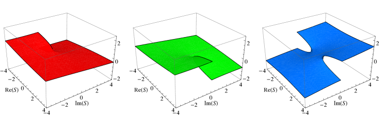
Figure 4: $\mathop{\rm Im}\nolimits\beta_{0}(S)$, $\mathop{\rm Im}\nolimits\beta_{1}(S)$, and $\mathop{\rm Im}\nolimits\beta_{2}(S)$ for $w=3/2^{2/3}$. For this value of $w$ the branch points are $S_{\pm}=\pm 1$.

In the three plots of figure 4 we show the imaginary parts $\mathop{\rm Im}\nolimits\beta_{0}(S)$, $\mathop{\rm Im}\nolimits\beta_{1}(S)$, and $\mathop{\rm Im}\nolimits\beta_{2}(S)$ respectively of the three branches of $\beta(S)$ for a fixed value $w=3/2^{2/3}$. This value of $w$ has been chosen because the corresponding branch points are $S_{\pm}=\pm 1$, and therefore easily identifiable in the figure. The upper and lower edges of the cuts along $\mathop{\rm Re}\nolimits S\leq S_{-}=-1$ of $\beta_{0}(S)$ (red surface) and $\beta_{2}(S)$ (blue surface) have to be glued, as well as the edges of the cuts along $\mathop{\rm Re}\nolimits S\geq S_{+}=1$ of $\beta_{1}(S)$ (green surface) and $\beta_{2}(S)$ (blue surface).

Thus, given a value of $S\neq S_{\pm}$, there are three values $\beta_{k}(S)$ from which we find three possible pairs of endpoints,

$$a_{k}(S)=\beta_{k}(S)-\sqrt{2S/\beta_{k}(S)},$$ (124)

$$b_{k}(S)=\beta_{k}(S)+\sqrt{2S/\beta_{k}(S)}.$$ (125)

Using (121) we find the expansions of $\beta_{k}(S)$ as $S\rightarrow 0$

$$\beta_{0}(S) = -\sqrt{w}-\frac{S}{2w}+\frac{3S^{2}}{8w^{5/2}}+\mathcal{O}(S^{3}),$$ (126)

$$\beta_{1}(S) = \sqrt{w}-\frac{S}{2w}-\frac{3S^{2}}{8w^{5/2}}+\mathcal{O}(S^{3}),$$ (127)

$$\beta_{2}(S) = \frac{S}{w}+\mathcal{O}(S^{3}).$$ (128)

Therefore according to our discussion in section 2.3, as $S\rightarrow 0$ the branches $\beta_{0}$ and $\beta_{1}$ represent families of one-cut spectral curves with a classical limit in which the cuts shrink to the critical point $-\sqrt{w}$ and $+\sqrt{w}$ of the cubic potential. Note also that the endpoints $a$ and $b$ can be expanded as Puiseux series. For example,

$$a_{1}^{\pm}(S)=\sqrt{w}\pm\frac{2^{1/2}S^{1/2}}{w^{1/4}}-\frac{S}{2w}\pm\frac{S^{3/2}}{2^{3/2}w^{7/4}}-\frac{3S^{2}}{8w^{5/2}}+\mathcal{O}(S^{5/2}),$$ (129)

where $a_{1}^{-}\equiv a$ and $a_{1}^{+}\equiv b$. The function $\beta_{2}(S)$ does not represents a family of spectral curves with a shrinking minimal cut as $S\rightarrow 0$ since it reduces to the solution (119) with $a_{2}^{\pm}\rightarrow\pm\sqrt{2w}$. We will see in sections 5.3 and 6.2 that there are not spectral curves with a minimal cut corresponding to $\beta_{2}(S)$ near $S=0$ and that the limit $S\rightarrow 0$ represents a critical spectral curve with two minimal cuts such that $S_{1}+S_{2}=0$.

The expression for the prepotential (82) takes, up to an unessential constant term $-w^{3}/12$, the following simple form in terms of the function $\beta(S)$

$$\mathcal{F}=\frac{\beta^{6}}{2}-\frac{5}{12}w\beta^{4}-\frac{(w\beta-\beta^{3})^{2}}{2}\mathop{\rm Log}\nolimits\left(\frac{w-\beta^{2}}{2}\right).$$ (130)

This expression for the prepotential is equivalent to previous results in which the first two terms in the right-hand side appear in rational form. For example, equation (51) in BR78 can be put in our polynomial form using equation (49) of BR78 to eliminate the denominator.

5.2 Superpotentials and the quantum parameter space

The one-cut case can be used to determine the vacua structure of the unbroken gauge group $U(N)$ FE03d . Using (130) and taking into account that

$$\frac{\partial\beta}{\partial S}=\frac{1}{w-3\beta^{2}},$$ (131)

the superpotential can be expressed in terms of $\beta$ as

$$W_{{\rm eff}} = -\frac{2}{3}N\beta^{3}-N(w\beta-\beta^{3})\mathop{\rm Log}\nolimits\left(\frac{w-\beta^{2}}{2}\right)+(w\beta-\beta^{3})\log\Lambda^{2N}$$ (132)

$$= -\frac{2}{3}N\beta^{3}+(w\beta-\beta^{3})\log\Big{(}\frac{2\,\Lambda^{2}}{w-\beta^{2}}\Big{)}^{N}.$$

We can obtain the vevs $\mathcal{S}$ since (85), (115) and (116) imply

$$(\delta^{(k)})^{2}=4\,\Lambda^{2}\zeta_{k},\quad\beta^{(k,\pm)}=\pm\,\sqrt{w-2\Lambda^{2}\zeta_{k}},\quad k=1,\ldots,N,$$ (133)

and

$$\mathcal{S}^{(k,\pm)}=\pm\,2\Lambda^{2}\zeta_{k}\sqrt{w-2\Lambda^{2}\zeta_{k}},\quad k=1,\ldots,N.$$ (134)

Hence we find two families of $N$ quantum vacua $|k,\pm\rangle$ which correspond to the two classical vacua $\pm\sqrt{w}$ of the cubic model.

To calculate the low-energy superpotential $W_{{\rm low}}(w,\Lambda)$ associated with the $|k,\pm\rangle$ vacua we notice that from (133) it follows that

$$\frac{2\Lambda^{2}\zeta_{k}}{w-(\beta^{(k,\pm)})^{2}}=1,$$ (135)

so that (132) leads to the following simple exact expression

$$W_{{\rm low}}^{(k,\pm)}=-\frac{2}{3}N(\beta^{(k,\pm)})^{3}=\mp\frac{2}{3}N(w-2\Lambda^{2}\zeta_{k})^{3/2}.$$ (136)

We can now calculate the vevs

$$\langle\mathop{\rm Tr}\nolimits\Phi\rangle^{(k,\pm)}=-\frac{\partial W_{{\rm low}}^{(k,\pm)}}{\partial w}=\pm N\sqrt{w-2\Lambda^{2}\zeta_{k}}=N\beta^{(k,\pm)},$$ (137)

and check that

$$\mathcal{S}^{(k,\pm)}=\frac{\partial W_{{\rm low}}^{(k,\pm)}}{\partial\log\Lambda^{2N}}=2\Lambda^{2}\beta^{(k,\pm)}\zeta_{k}.$$ (138)

In this way we have that the one-cut sector $\mathcal{M}_{\rm q}^{(1)}$ of the quantum parameter space can be decomposed into $N$ subsets

$$\mathcal{M}_{\rm q}^{(1)}=\cup_{k=1}^{N}\mathcal{M}_{\rm q}^{(1,k)},$$ (139)

where $\mathcal{M}_{\rm q}^{(1,k)}$ is represented by the two-sheeted Riemann surface of the function $\sqrt{w-\lambda}$. Here

$$\lambda=2\Lambda^{2}\zeta_{k}.$$ (140)

The two sheets $\mathcal{M}_{\rm q}^{(1,k,\pm)}$ are connected through the branch cuts emerging from $\lambda=w$. Each point $(\lambda,\pm)\in\mathcal{M}_{\rm q}^{(1,k,\pm)}$ determines a unique spectral curve given by

$$S=\pm\lambda\sqrt{w-\lambda},\quad\beta=\pm\sqrt{w-\lambda},\quad\delta^{2}=2\lambda.$$ (141)

5.3 Critical spectral curves in the complex $S$ plane

In this section we derive an analytic condition met by critical curves in the complex $S$ plane, i.e., by the locus of values of the complex ’t Hooft parameter $S$ that yield critical spectral curves with minimal cuts. Let us denote by $\Sigma_{k}(S)$ the families of one-cut spectral curves corresponding to the branches $\beta_{k}(S)$ for $k=0,1,2$. The minimal cuts of $\Sigma_{k}(S)$ for a fixed value of $S$ are Stokes lines defined by

$$\mathop{\rm Re}\nolimits G_{k}(z)=0$$ (142)

where

$$G_{k}(z)=\mathrm{e}^{-\mathrm{i}\arg S}\int_{a_{k}^{-}}^{z^{\prime}}\left(z^{\prime}+\beta_{k}\right)\sqrt{(z^{\prime}-\beta_{k})^{2}-\delta_{k}^{2}}\,\mathrm{d}z^{\prime}.$$ (143)

Therefore, if for a certain value of $S$ the double zero $-\beta_{k}$ of $y(z)$ meets the Stokes line, i.e., if

$$\mathop{\rm Re}\nolimits G_{k}(-\beta_{k})=0,$$ (144)

the curve has a critical point. In fact, we can find an analytic condition (which, however, has to be solved numerically) for this critical behavior, because the integrals (143) can be evaluated in closed form. Thus, we find that the critical curve in the complex $S$-plane corresponding to a branch $\beta_{k}(S)$ is given by

$$\mathop{\rm Re}\nolimits\left[\frac{w}{3S}\sqrt{6\beta_{k}^{2}-2w}+\log\left(\sqrt{\frac{\beta_{k}}{2S}}\left(-2\beta_{k}+\sqrt{6\beta_{k}^{2}-2w}\right)\right)\right]=0.$$ (145)

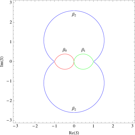
Figure 5: Critical curves in the sense that $\mathop{\rm Re}\nolimits G_{k}(-\beta(S))=0$ for $w=3/2^{2/3}$. Each arc is marked with the corresponding branch $\beta_{k}$ and drawn in the color matching the corresponding branch in figure 4.

In figure 5 we show the three branches $\mathop{\rm Re}\nolimits G_{k}(-\beta)=0\,(k=0,1,2)$ obtained by numerical solution of (145) for $w=3/2^{2/3}$. Each arc is marked and colored to match the corresponding branch $\beta_{k}$ in figure 4 (e.g., the red critical curve, marked $\beta_{0}$, lies on the first plot of figure 4). We have performed extensive numerical calculations of the corresponding Stokes graphs, from which we infer the following picture.

Consider first the branch $\beta_{2}(S)$. The critical (blue) curve in figure 5 separates the $S$ plane into a bounded region and an unbounded region. In the unbounded region we always find a minimal cut joining $a$ to $b$, and therefore a one-cut solution. The critical (blue) line corresponds to configurations where the double root $-\beta_{2}$ meets the minimal cut, and in the bounded region of the $S$ plane the Stokes graphs do not feature finite Stokes lines, i.e., there are not one-cut spectral curves with a minimal cut in this branch. This behavior is illustrated in figure 6, where we show the Stokes graphs for $w=3/2^{2/3}$ and three values of $S$: $S=-0.5-\mathrm{i}\,3$, in the unbounded region of the $S$ plane and slightly below the blue critical curve, $S=-0.5-\mathrm{i}\,2.514\,668\ldots$ on the critical curve, and $S=-0.5-\mathrm{i}\,2$ in the bounded region of the $S$ plane but slightly above the critical curve. Numerical calculations to be presented in the next section show that these critical configurations can be continued to spectral curves with two minimal cuts. Thus, crossing the blue critical curve from the bounded to the unbounded region would correspond to a “merging of two minimal cuts” in the terminology of random matrix theory.

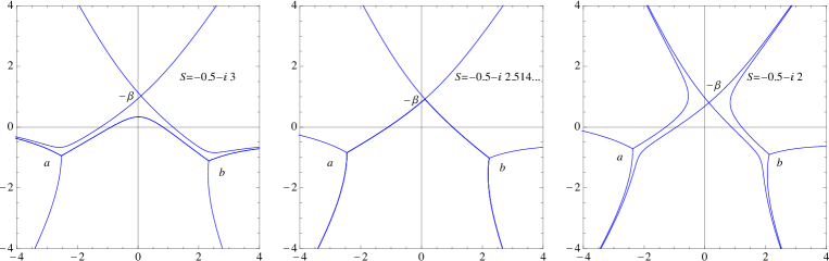
Figure 6: Stokes complexes on the branch $\beta_{2}(S)$ for $w=3/2^{2/3}$ and three values of $S$: $S=-0.5-\mathrm{i}\,3$ (slightly below the blue critical curve in figure 5), $S=-0.5-\mathrm{i}\,2.514\,668\ldots$ (on the critical curve), and $S=-0.5-\mathrm{i}\,2$ (slightly above the critical curve).

The behavior of the branches $\beta_{0}(S)$ and $\beta_{1}(S)$ is the same, and qualitatively different from the behavior of $\beta_{2}(S)$. For concreteness we will describe the behavior of $\beta_{0}(S)$. The corresponding critical curve (the red curve in figure 5) separates the $S$ plane into a bounded region and an unbounded region. In the unbounded region we always find a minimal cut joining $a$ to $b$. The critical curve corresponds to configurations where the double root $-\beta_{0}$ does not meet the minimal cut joining $a$ to $b$, but a second finite Stokes line joining $b$ to $-\beta_{0}$ appears. However, if we proceed to the bounded region of the $S$ plane the Stokes graphs again feature a finite Stokes line joining $a$ to $b$, i.e., there are one-cut solutions with a minimal cut. This behavior is illustrated in figure 7, where we show the Stokes graphs for $w=3/2^{2/3}$ and three values of $S$: $S=-0.5-\mathrm{i}\,0.5$, in the unbounded region of the $S$ plane and slightly below the red critical curve, $S=-0.5-\mathrm{i}\,0.388\,126\ldots$ on the critical curve, and $S=-0.5-\mathrm{i}\,0.3$ in the bounded region of the $S$ plane but slightly above the critical curve. Numerical calculations to be presented in the next section also show that crossing the critical curve of the $S$ plane in the $\beta_{0}$ branch from the unbounded to the bounded region we can continue with one-cut solutions with a minimal cut (as illustrated in figure 7) or alternatively we can continue from the critical configuration to a spectrum curve with two minimal cuts. In this sense, crossing the red critical curve from the bounded to the unbounded region may correspond either to no phase change or to a “birth of a minimal cut at a distance” in the terminology of random matrix theory EY06 .

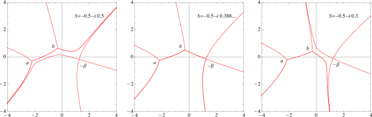
Figure 7: Stokes complexes on the branch $\beta_{0}(S)$ for $w=3/2^{2/3}$ and three values of $S$: $S=-0.5-\mathrm{i}\,0.5$ (slightly below the red critical curve in figure 5), $S=-0.5-\mathrm{i}\,0.388\,126\ldots$ (on the critical curve), and $S=-0.5-\mathrm{i}\,0.3$ (slightly above the critical curve).

5.4 Spectral curves with one minimal cut in the quantum parameter space

In the case of the cubic model each point $(\lambda,\pm)\in\mathcal{M}_{\rm q}^{(1,k,\pm)}$ determines a spectral curve (141) which will be critical if it satisfies the condition (145) or, equivalently, in terms of the variable $\lambda$

$$\mathop{\rm Re}\nolimits\left[\pm\frac{w}{3\lambda}\frac{\sqrt{4w-6\lambda}}{\sqrt{w-\lambda}}+\log\left(\frac{\sqrt{4w-6\lambda}\mp 2\sqrt{w-\lambda}}{\sqrt{2\lambda}}\right)\right]=0.$$ (146)

This equation defines a curve in $\mathcal{M}_{\rm q}^{(1,k,\pm)}$ and since

$$\left(\frac{\sqrt{4w-6\lambda}-2\sqrt{w-\lambda}}{\sqrt{2\lambda}}\right)\left(\frac{\sqrt{4w-6\lambda}+2\sqrt{w-\lambda}}{\sqrt{2\lambda}}\right)=-1,$$ (147)

the parts of the curve lying in each sheet $\mathcal{M}_{\rm q}^{(1,k,+)}$ and $\mathcal{M}_{\rm q}^{(1,k,-)}$ are identical. Figure 8 shows that this critical curve is composed of two ovals, one of them containing the branch point $\lambda=w$.

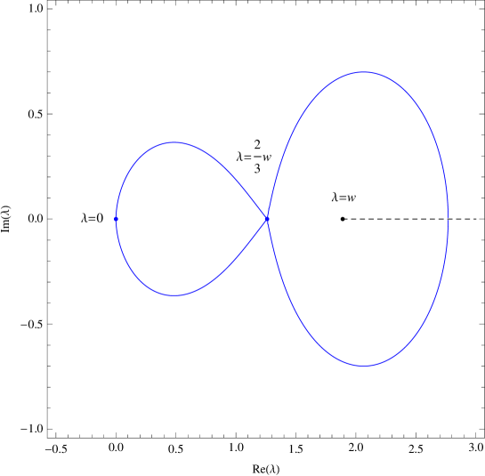
Figure 8: Critical curve in $\mathcal{M}_{\rm q}^{(1,k,\pm)}$ for $w=3/2^{2/3}$.

It is not difficult to give an argument that suggests which regions of the sheets $\mathcal{M}_{\rm q}^{(1,k,\pm)}$ correspond to spectral curves with one minimal cut:

1. As $\lambda\to 0$ then $S(\lambda)\to 0$ and $\beta(\lambda)\to\sqrt{w}$. Therefore, according to (127), the function $\beta(\lambda)$ near $\lambda=0$ behaves as $\beta_{1}(S)$ near $S=0$.

2. As $\lambda\to w$ then $S(\lambda)\to 0$ and $\beta(\lambda)\to 0$. Therefore, according to (128), the function $\beta(\lambda)$ near $\lambda=w$ behaves as $\beta_{2}(S)$ near $S=0$.

As a consequence, the analysis in sec. 5.3 permits us to conjecture that the points in the interior of the oval containing $\lambda=w$ do not supply spectral curves with one minimal cut, and that the oval itself describes processes of splitting of a cut. Conversely, points in the interior of the leftmost oval determine spectral curves with one minimal cut and points on the oval lead to critical spectral curves describing birth of a cut at a distance. Finally, since as $\lambda\to\infty$ then $S(\lambda)\to\infty$ so that according to the analysis in sec. 5.3 we expect that points outside the critical ovals determine spectral curves with one minimal cut.

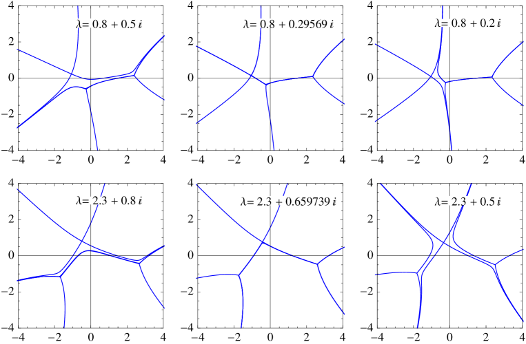
Figure 9: Stokes complexes for two paths in $\mathcal{M}_{\rm q}^{(1,k,\pm)}$ which enter vertically from above the left oval (first row) and the right oval (second row) of the critical curve of figure 8.

These arguments are supported by numerical calculations, two of which are illustrated in figure 9. The three graphs in the first row correspond to three values of $\lambda$ on the same vertical $\mathop{\rm Re}\nolimits\lambda=0.8$. The first value is above the left oval, the second value is critical, i.e., on this oval, and the third value is already in the interior of the oval. These graphs show how we proceed from a spectral curve with one minimal cut, through a critical configuration (in which the three turning points are joined by finite Stokes lines), to another spectral curve with one minimal cut. The three graphs in the second row correspond to three values of $\lambda$ on the vertical $\mathop{\rm Re}\nolimits\lambda=2.3$. The first value is above the right oval, the second value is critical, i.e., on this oval, and the third value is already in the interior of the oval. Now the graphs show that we proceed from a spectral curve with one minimal cut, through a critical configuration (in which the three turning points are joined by finite Stokes lines), but that as we enter the interior of the oval it does not exist an spectral curve with one minimal cut.

As we discussed in section 4.3 critical spectral curves describing a splitting of a cut process determine interpolating points between the sectors $\mathcal{M}_{\rm q}^{(1)}$ and $\mathcal{M}_{\rm q}^{(2)}$ of the quantum parameter space. Therefore for the cubic model the ovals containing $\lambda=w$ in the sheets $\mathcal{M}_{\rm q}^{(1,k,\pm)}$ are interpolating curves between the subsets of these sectors corresponding to spectral curves with minimal cuts. These results show a structure of the quantum parameter space drastically different from that found in FE03d where, due to the absence of a concrete choice of the cuts, the only interpolation found between the sectors $\mathcal{M}_{\rm q}^{(1)}$ and $\mathcal{M}_{\rm q}^{(2)}$ is the single point $\lambda=w$. However, as it will be proved in section 6.2, this point describes a merging of two minimal cuts into a non minimal cut.

6 Two-cut spectral curves in the cubic model

In this section we consider the two-cut phase of spectral curves for the cubic potential (113). We first derive the series expansions around the critical points of the potential for the endpoints of two-cut spectral curves with classical limit. Then we discuss the particular solution corresponding to the slice $S_{1}+S_{2}=0$. Finally, we describe a numerical method to calculate spectral curves with two minimal cuts and their critical processes.

6.1 Endpoints and series expansions

In the two-cut case we will denote $a_{1}^{-}\equiv a$, $a_{1}^{+}\equiv b$, $a_{2}^{-}\equiv c$ and $a_{2}^{+}\equiv d$. Following again the procedure outlined in section 2.1 the corresponding $y$ function to be substituted in (5) has the form

$$y(z)=\sqrt{(z-a)(z-b)(z-c)(z-d)},$$ (148)

and $f(z)=-4(S_{1}+S_{2})z+b_{0}$. The equations for the possible endpoints turn out to be

$$abc+abd+acd+bcd = 4(S_{1}+S_{2}),$$ (149)

$$ab+ac+ad+bc+bd+cd = -2w,$$ (150)

$$a+b+c+d = 0,$$ (151)

$$I(a,b,c,d) = 2\pi\mathrm{i}S_{1},$$ (152)

where

$$I(a,b,c,d)=\int_{a}^{b}\sqrt{(z_{+}-a)(z_{+}-b)(z_{+}-c)(z_{+}-d)}\,\mathrm{d}z.$$ (153)

Although (153) can be expressed in terms of elliptic integrals it is clear that, except in specially simple particular cases, the system (149)–(152) cannot be solved in closed form. However, we can characterize solutions that have a classical limit by means of their series expansions for the endpoints that tend to the critical points $\pm\sqrt{w}$ of the cubic potential as $S_{1}$ and $S_{2}$ tend to zero. These series are the analog of equation (129) in the one-cut case. Since in the two-cut case we lack closed-form solutions analog to (121), we resort to direct substitution of suitable Puiseux expansion into equations (149)–(152). We do have, however, an scaling relation analog to (120):

$$a(w,S_{1},S_{2})=w^{1/2}a(1,S_{1}/w^{3/2},S_{2}/w^{3/2}),$$ (154)

with similar relations for $b$, $c$ and $d$. Therefore we can write the following Puiseux expansions:

$$a = \sqrt{w}\left(-1+\sum_{j=1}^{\infty}\frac{a_{j}}{w^{3j/4}}\right),$$ (155)

$$b = \sqrt{w}\left(-1+\sum_{j=1}^{\infty}\frac{(-1)^{j}a_{j}}{w^{3j/4}}\right),$$ (156)

$$c = \sqrt{w}\left(1+\sum_{j=1}^{\infty}\frac{c_{j}}{w^{3j/4}}\right),$$ (157)

$$d = \sqrt{w}\left(1+\sum_{j=1}^{\infty}\frac{(-1)^{j}c_{j}}{w^{3j/4}}\right),$$ (158)

where we have separated explicitly the first term to identify $a$ and $b$ as the endpoints of the cut that opens up from $-\sqrt{w}$ and $c$ and $d$ as the endpoints of the cut that opens up from $\sqrt{w}$, and where the coefficients $a_{j}$ and $c_{j}$ are functions of $S_{1}$ and $S_{2}$. Substitution of these series into the first three equations (149)–(151) is straightforward. As to the fourth equation (152), which involves the integral (153), we can formally fix the endpoints of the contracting integration interval with a linear change of variable

$$I(a,b,c,d)=-\mathrm{i}(b-a)^{2}\sqrt{(c-a)(d-a)}\int_{0}^{1}\sqrt{t(1-t)}r_{ab}(t)\mathrm{d}t,$$ (159)

where

$$r_{ab}(t)=\sqrt{\left(1-\frac{b-a}{c-a}t\right)\left(1-\frac{b-a}{d-a}t\right)}.$$ (160)

Then we expand $r_{ab}(t)$ as a power series in $t$ around $t=0$ (recall that $b-a$ tends to zero while the denominators remain finite) and integrate term by term. All the integrals are of the form

$$\int_{0}^{1}\sqrt{t(1-t)}t^{k}\,\mathrm{d}t=\frac{\sqrt{\pi}}{2}\frac{\Gamma(k+3/2)}{\Gamma(k+3)},\quad k=0,1,2,\ldots$$ (161)

and the substitution of the Puiseux series for $a$, $b$, $c$, and $d$ in the resulting expression is again straightforward.

To illustrate the pattern of the resulting Puiseux series we show the first six coefficients $a_{k}$ and $c_{k}$:

$$a_{1} = \mathrm{i}\sqrt{2S_{1}},$$ (162)

$$a_{2} = \frac{1}{2}(-{S_{1}}+{S_{2}}),$$ (163)

$$a_{3} = -\mathrm{i}\frac{\sqrt{2S_{1}}}{8}(2{S_{1}}-3{S_{2}}),$$ (164)

$$a_{4} = \frac{1}{8}(3S_{1}^{2}-8{S_{1}}{S_{2}}+3S_{2}^{2}),$$ (165)

$$a_{5} = \mathrm{i}\frac{\sqrt{2S_{1}}}{128}(36S_{1}^{2}-122S_{1}S_{2}+69S_{2}^{2}),$$ (166)

$$a_{6} = -\frac{1}{32}({S_{1}}-{S_{2}})(16S_{1}^{2}-59S_{1}S_{2}+16S_{2}^{2}),$$ (167)

$$c_{1} = -\sqrt{2S_{2}},$$ (168)

$$c_{2} = \frac{1}{2}({S_{1}}-{S_{2}}),$$ (169)

$$c_{3} = \frac{\sqrt{2S_{2}}}{8}(3{S_{1}}-2{S_{2}}),$$ (170)

$$c_{4} = -\frac{1}{8}(3S_{1}^{2}-8S_{1}S_{2}+3S_{2}^{2})$$ (171)

$$c_{5} = -\frac{\sqrt{2S_{2}}}{128}(69S_{1}^{2}-122S_{1}S_{2}+36S_{2}^{2}),$$ (172)

$$c_{6} = \frac{1}{32}({S_{1}}-{S_{2}})(16S_{1}^{2}-59S_{1}S_{2}+16S_{2}^{2}).$$ (173)

The odd coefficients $a_{k}$ and $c_{k}$ involve the square roots of the corresponding ’t Hooft parameters (and cancel in the series for the differences $b-a$ and $d-c$), while the even coefficients are homogeneous polynomials of degree $k/2$ in $S_{1}$ and $S_{2}$. Note also that if in the expressions for the $a_{k}$ we set $S_{1}=0$ and $S_{2}=S$ we formally recover the one-cut expansions (129).

6.2 The cubic model on the slice $S_{1}+S_{2}=0$

As an explicit application of the endpoint equations (149)–(152) we describe now the two-cut spectral curves of the cubic model in the Seiberg-Witten slice $S_{1}+S_{2}=0$ SE94 . These configurations have been used in the literature to study the phase structure of brane/anti-brane systems at large $N$ and non-perturbative effects in matrix models CA07 ; HE07 ; HE08 ; KL10 . We look for solutions of (149)–(152) satisfying

$$c=-b,\quad d=-a,$$ (174)

where we assume $|a|>|b|$. Then these equations reduce to

$$a^{2}+b^{2}=2w,$$ (175)

$$\int_{a}^{b}\sqrt{(z_{+}^{2}-a^{2})(z_{+}^{2}-b^{2})}\mathrm{d}z=2\pi\mathrm{i}S_{1}.$$ (176)

We may solve (175) in the form

$$a=|a|\mathrm{e}^{\mathrm{i}\arg w/2},\quad b=|b|\mathrm{e}^{\mathrm{i}\arg w/2},\quad|b|=\sqrt{2|w|-|a|^{2}},$$ (177)

and it is immediate to see that the straight line segments $[a,b]$ and $[c,d]$ are minimal cuts provided that

$$\arg S_{1}=\frac{3}{2}\arg w.$$ (178)

In particular (176) reads

$$\int_{\sqrt{2|w|-|a|^{2}}}^{|a|}\sqrt{(x^{2}-|a|^{2})(x^{2}+|a|^{2}-2|w|)}\mathrm{d}x=2\pi\mathrm{i}|S_{1}|,$$ (179)

which gives $|S_{1}|$ as a function of $|a|$.

Therefore (178) determines a family of spectral curves $\Sigma(\gamma,S_{1},S_{2}=-S_{1})$ with two minimal cuts, parameterized by the values of $|a|$ in the interval $[\sqrt{|w|},\sqrt{2|w|}]$. The limit $|a|\rightarrow\sqrt{2|w|}$ of this family deserves a particular attention since the spectral curve reduces to the one-cut solution (128) determined by

$$S=0,\quad\beta=0,\quad\delta^{2}=2w.$$ (180)

However due to the fact that $\arg S_{1}\neq\arg S_{2}$ the cut resulting from the merging is not a minimal cut. This spectral curve corresponds to the singular point $\lambda=w$ of the quantum parameter space $\mathcal{M}_{\rm q}^{(1)}$ at which the solutions $\mathcal{S}^{(k)}(\Lambda^{2})$ of the field equation are not analytic, as it should be expected since $h(z)=z+\beta$ and the condition (86) is satisfied.

6.3 Numerical calculation of minimal cuts and critical processes

A direct numerical solution of the system (149)–(152) without a suitable, well identified initial point would be extremely difficult (note that for a fixed value of $w$ the endpoints are functions of the two complex variables $S_{1}$ and $S_{2}$). However, we can take advantage of our knowledge of the critical curve (145) and the corresponding explicit solutions for the one-cut endpoints given by (121), (124) and (125), and proceed iteratively by small increments in $S_{1}$ and $S_{2}$ to calculate the solutions of (149)–(152) at any desired pair of values $(S_{1},S_{2})$ using as initial approximation at each step the results of the previous one.

To illustrate this approach, consider the second, critical configuration in figure 6. In figure 10 we show the numerical continuation from this critical configuration into the two-cut region for two examples. In the first graph of figure 10 we have set $S_{1}=S_{2}=99S/200$, where $S=-0.5-\mathrm{i}\,2.514\,668\ldots$ is the critical value in figure 6. Note that $S_{1}+S_{2}$ is a small perturbation of $S$ (cf. equation (98)), i.e., we split the double zero $-\beta$ into two simple zeros of $y(z)^{2}$ and the critical Stokes graph into a a graph with two finite Stokes lines of similar length (recall that the critical configuration is not symmetric) with $\arg(S_{1})=\arg(S_{2})$. Since the corresponding functions $G_{j}(z)$ in (28) have the same values of $\arg S_{j}$, the Stokes lines cannot cross. Similarly, in the second graph of figure 10 we have perturbed slightly this solution to $S_{1}=99S/200$ and $S_{2}=\mathrm{e}^{\mathrm{i}\pi/25}S_{1}$. Now $\arg S_{1}\neq\arg S_{2}$ and two of the Stokes lines corresponding to different values of $j$ do cross. As we anticipated in the previous section, looking at this process backwards we have an instance of a “merging of two minimal cuts” in the terminology of random matrix theory.

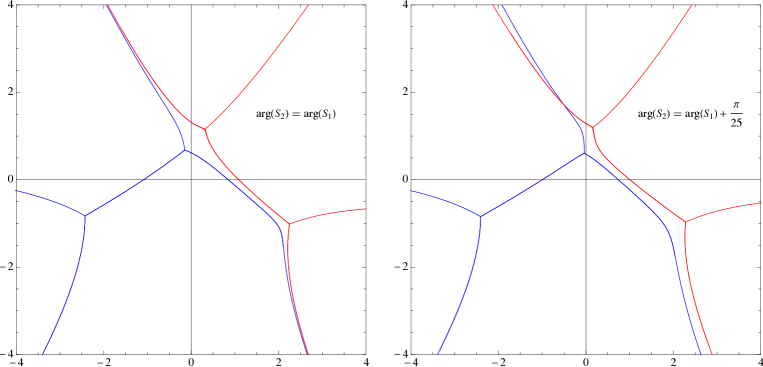
Figure 10: Stokes complexes in the two-cut region for $w=3/2^{2/3}$ and two pairs $(S_{1},S_{2})$ close to the critical curve: the first graph corresponds to $S_{1}=S_{2}=99S/200$, where $S=-0.5-\mathrm{i}\,2.514\,668\ldots$ is the critical value in figure 6 (note that in this case $\arg(S_{1})=\arg(S_{2})$ and the Stokes lines do not cross); the second graph corresponds to $S_{1}=99S/200$ and $S_{2}=\mathrm{e}^{\mathrm{i}\pi/25}S_{1}$ (note that in this case $\arg(S_{1})\neq\arg(S_{2})$ and two Stokes lines cross).

Likewise, in figure 11 we illustrate the numerical continuation from the critical configuration in the second graph of figure 7 to the two-cut region. In the first graph of figure 11 we have set $S_{1}=S$, $S_{2}=S/10$, where $S=-0.5-\mathrm{i}\,0.388\,126\ldots$ is the critical value in figure 7. Again, this is a small perturbation of the critical configuration which we use to generate the initial approximation. The double zero $-\beta$ splits into two simple zeros and the critical Stokes graph into a graph with a long finite Stokes line corresponding to $S_{1}$ and a short finite Stokes line corresponding to $S_{2}$. Since in this first graph we have taken $\arg(S_{1})=\arg(S_{2})$, the corresponding functions $G_{j}(z)$ in (28) have the same values of $\arg S_{j}$, and the Stokes lines cannot cross. In the second graph we have increased the argument of $S_{2}$ by $\pi/30$, and two Stokes lines corresponding to different values of $j$ cross. As we anticipated in the previous section this is an instance of a “birth of a minimal cut at a distance” in the terminology of random matrix theory.

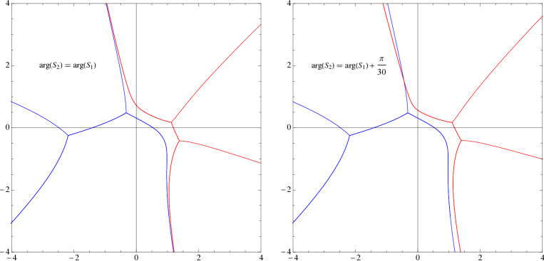
Figure 11: Stokes complexes in the two-cut region for $w=3/2^{2/3}$ and two pairs $(S_{1},S_{2})$ close to the critical curve: the first graph corresponds to $S_{1}=S$, $S_{2}=S/10$, where $S=-0.5-\mathrm{i}\,0.388\,126\ldots$ is the critical value in figure 7; (note that in this case $\arg(S_{1})=\arg(S_{2})$ and the Stokes lines do not cross); the second graph corresponds to $S_{1}=S$ and $S_{2}=\mathrm{e}^{\mathrm{i}\pi/30}S/10$ (note that in this case $\arg(S_{1})\neq\arg(S_{2})$ and two Stokes lines cross).

Therefore we have an efficient numerical algorithm that taking critical one-cut solutions as data to generate an initial approximation to solve equations (149)–(152), allows us to proceed stepwise tracking the solution along any specified path of the complex variables $S_{1}$ and $S_{2}$, generate the two-cut endpoints $a(S_{1},S_{2})$, $b(S_{1},S_{2})$, $c(S_{1},S_{2})$, $d(S_{1},S_{2})$ and calculate the corresponding Stokes graph.

7 Summary

In this paper we have presented a self-contained approach to study the phase transitions that arise in the study of large $N$ dualities between $\mathcal{N}=1$ SUSY $U(N)$ gauge theories and string models on local Calabi-Yau manifolds. Conceptually, it is based on the use of spectral curves with branch cuts that are projections of minimal supersymmetric cycles. From the practical point of view, the key elements of our approach are a system of equations for the branch points and a characterization of the branch cuts as Stokes lines of a suitable set of polynomials. The system of equations for the branch points is derived from the form of the equation of the spectral curve with a fixed number of cuts after imposing period relations on the cuts. In turn, these branch cuts are a natural generalization of the cuts that define the eigenvalue support in holomorphic matrix models (note that in this latter case the partial ’t Hooft parameters are essentially the eigenvalue fractions and therefore real and positive). However, we do not rely on any underlying matrix model but use a variational characterization of the (in general complex) density as an extremal of a prepotential naturally associated to the spectral curve. By writing the derivatives of the prepotential with respect to the ’t Hooft parameters in terms of Abelian integrals we study the splitting of a cut in the space of spectral cuts and show it is typically a third order transition. We also show that a critical spectral curve corresponding to the splitting of a cut represents an interpolating points between different sectors in the quantum parameter space. We have applied these theoretical results and numerical calculations to study the cubic model, finding the analytic condition satisfied by critical one-cut spectral curves, and characterizing the transition curves between the one-cut and two-cut phases both in the space of spectral curves and in the quantum parameter space. Although our analytic results in the one-cut phase of the cubic model rely on the explicit solution of a cubic equation, in principle nothing prevents the use of the same numerical methods used in the two-cut phase to study spectral curves for non polynomial potentials.

A Prepotential identities

In this appendix we collect the proofs of the main identities satisfied by the prepotential associated to spectral curves. To prove (67) and (68) we differentiate (50) with respect $S_{i}$ taking into account that $\rho(a_{1}^{\pm})=\cdots=\rho(a_{s}^{\pm})=0$. Thus we have

$$\frac{\partial\mathcal{F}}{\partial S_{i}} = \int_{\gamma}W(z)\frac{\partial\mathrm{d}q(z)}{\partial S_{i}}-\int_{\gamma}\int_{\gamma}\mathop{\rm Log}\nolimits(z-z^{\prime})^{2}\mathrm{d}q(z^{\prime})\frac{\partial\mathrm{d}q(z)}{\partial S_{i}}$$ (181)

$$= \int_{\gamma}\left(W(z)-(g(z_{+})+g(z_{-}))\right)\frac{\partial\mathrm{d}q(z)}{\partial S_{i}}$$

$$= \sum_{j=1}^{s}L_{j}\int_{\gamma_{j}}\frac{\partial\mathrm{d}q(z)}{\partial S_{i}}=L_{i},$$

where we have used (48) and the fact that because of (10)

$$\int_{\gamma_{j}}\frac{\partial\mathrm{d}q(z)}{\partial S_{i}}=\frac{\partial}{\partial S_{i}}\int_{\gamma_{j}}\mathrm{d}q(z)=\delta_{ij}.$$ (182)

Moreover, from (48) we have that

$$L_{j}=W(z_{j})-\int_{\gamma}\mathop{\rm Log}\nolimits(z-z_{j})^{2}\,\mathrm{d}q(z),\quad z_{j}\in\gamma_{j},$$ (183)

and (67) and (68) follow immediately.

We will next prove that the asymptotics of $L_{j}$ in the classical limit is

$$L_{j}\sim W(a_{j})-\sum_{k\neq j}S_{k}\,\log\Delta_{jk}^{2}+S_{j}\Big{(}1+\log\Big{(}\frac{W^{\prime\prime}(a_{j})}{S_{j}}\Big{)}\Big{)},$$ (184)

where $\Delta_{jk}\equiv a_{j}-a_{k}$. To this aim we set $z_{j}=a_{j}^{+}$ in (183) and get

$$L_{j}=W(a_{j}^{+})-\frac{1}{2\,\pi\,i}\int_{\gamma}{\rm Log}(z-a_{j}^{+})^{2}\,y(z_{+})\mathrm{d}z.$$ (185)

The classical limit of the first term is

$$W(a_{j}^{+})=W(\beta_{j}+\delta_{j})\sim W(a_{j}+\delta_{j})\sim W(a_{j})+\frac{W^{\prime\prime}(a_{j})}{2}\delta_{j}^{2}.$$ (186)

The second term decomposes as a sum

$$\int_{\gamma}{\rm Log}(z-a_{j}^{+})^{2}y(z_{+})\mathrm{d}z=\sum_{k}\int_{\gamma_{k}}{\rm Log}(z-a_{j}^{+})^{2}y(z_{+})\mathrm{d}z.$$ (187)

Taking into account the periods (7), for $k\neq j$ we get

$$\int_{\gamma_{k}}{\rm Log}(z-a_{j}^{+})^{2}y(z_{+})\mathrm{d}z\sim\mathop{\rm Log}\nolimits(\Delta_{jk}^{2})\int_{\gamma_{k}}y(z_{+})\mathrm{d}z=2\pi\mathrm{i}S_{k}\mathop{\rm Log}\nolimits(\Delta_{jk}^{2}),\quad k\neq j.$$ (188)

Moreover, using (34) we obtain

$$\int_{\gamma_{j}}\mathop{\rm Log}\nolimits(z-a_{j}^{+})^{2}y(z_{+})\mathrm{d}z\sim\mathrm{i}W^{\prime\prime}(a_{j})\int_{a_{j}^{-}}^{a_{j}^{+}}\mathop{\rm Log}\nolimits(z-a_{j}^{+})^{2}\sqrt{(z-a_{j}^{-})(a_{j}^{+}-z)}\mathrm{d}z.$$ (189)

The integral in the right-hand side can be exactly calculated using the change of variables $z=a_{j}^{-}+(a_{j}^{+}-a_{j}^{-})\,t$:

$$\int_{a_{j}^{-}}^{a_{j}^{+}}{\rm Log}(z-a_{j}^{+})^{2}\sqrt{(z-a_{j}^{-})(a_{j}^{+}-z)}\mathrm{d}z$$

$$=4\delta_{j}^{2}\mathop{\rm Log}\nolimits(4\delta_{j}^{2})\int_{0}^{1}\sqrt{t(1-t)}\mathrm{d}t+4\delta_{j}^{2}\int_{0}^{1}\mathop{\rm Log}\nolimits(t-1)^{2}\sqrt{t(1-t)}\mathrm{d}t$$

$$=\pi\frac{\delta_{j}^{2}}{2}\mathop{\rm Log}\nolimits(4\delta_{j}^{2})+\pi\frac{\delta_{j}^{2}}{2}(1-\mathop{\rm Log}\nolimits 16)$$

$$=\pi\frac{\delta_{j}^{2}}{2}\Big{(}1+\mathop{\rm Log}\nolimits\frac{\delta_{j}^{2}}{4}\Big{)}$$ (190)

Hence using (37) the asymptotics (184) follows.

Let us prove now the expression (75) of the second derivatives of the prepotential in terms of Abelian integrals. Differentiating (183) we find that

$$\frac{\partial^{2}\mathcal{F}}{\partial S_{i}\partial S_{j}}=\frac{\partial L_{i}}{\partial S_{j}}=-\int_{\gamma}\mathop{\rm Log}\nolimits(z-z_{i})^{2}\frac{\partial\mathrm{d}q(z)}{\partial S_{j}},\quad z_{i}\in\gamma_{i},$$ (191)

where the integrals are independent of the choice of $z_{i}$ in $\gamma_{i}$. From (45) and (7) it follows that

$$\frac{\partial}{\partial S_{j}}\mathrm{y}(z)\mathrm{d}z=-4\pi\mathrm{i}(1-\delta_{js})\mathrm{d}\phi_{j}-2\mathrm{d}\Omega_{0}.$$ (192)

Hence

$$\frac{\partial\mathrm{d}q(z)}{\partial S_{j}}=-2(1-\delta_{js})\mathrm{d}\phi_{j}(z_{+})-\frac{1}{\pi\mathrm{i}}\mathrm{d}\Omega_{0}(z_{+}).$$ (193)

Substituting (193) into (191) we get

$$\frac{\partial^{2}\mathcal{F}}{\partial S_{i}\partial S_{j}} = 2(1-\delta_{js})\int_{\gamma}\mathop{\rm Log}\nolimits(z-z_{i})^{2}\mathrm{d}\phi_{j}(z_{+})$$ (194)

$${}+\frac{1}{\pi\mathrm{i}}\int_{\gamma}\mathop{\rm Log}\nolimits(z-z_{i})^{2}\mathrm{d}\Omega_{0}(z_{+}),\quad z_{i}\in\gamma_{i}.$$

Consider now the first integral in the right-hand side of (194) and denote

$$F_{j}(u)=\int_{\gamma}\mathop{\rm Log}\nolimits(z-u)^{2}\mathrm{d}\phi_{j}(z_{+}),\quad u\in\gamma.$$ (195)

It follows from (71) that

$$\mathrm{d}\phi_{j}(z_{+})=-\mathrm{d}\phi_{j}(z_{-}),\quad z\in\gamma,$$ (196)

which implies that

$$F_{j}(u) = \int_{\gamma}(\log(z_{+}-u)+\log(z_{-}-u))\mathrm{d}\phi_{j}(z_{+})$$ (197)

$$= -\int_{A}\log(z-u)\mathrm{d}\phi_{j}(z),$$

where $A=A_{1}+\cdots+A_{s}$ is the sum of the contours in figure 1. Therefore

$$F^{\prime}_{j}(u)=\int_{A}\frac{\mathrm{d}\phi_{j}(z)}{z-u}=0,\quad u\in\gamma,$$ (198)

because the integrand is analytic outside $A$ and has residue zero at $\infty$. Therefore the functions $F_{j}(u)$ are constant on any connected piece of $\gamma$. Moreover, equation (197) shows that the functions $F_{j}(u)$ are analytic in $\mathbb{C}\setminus\Gamma$ and

$$F^{\prime}_{j}(u)=\int_{A}\frac{\mathrm{d}\phi_{j}(z)}{z-u}=-2\pi\,\mathrm{i}\,\frac{p_{j}(u)}{w(u)},\quad u\notin\gamma.$$ (199)

Since

$$\int_{A}\mathrm{d}\phi_{j}(z)=0,$$ (200)

it also follows from (197) that $F_{j}(u)=\mathcal{O}(1/u)$ as $u\rightarrow\infty$. Therefore, using the standard definition of the Abelian integrals

$$\phi_{j}(u)=\int_{\infty_{1}}^{u}\mathrm{d}\phi_{j}(z)$$ (201)

and equation (199), we may write

$$F_{j}(u)=-2\pi\mathrm{i}\phi_{j}(u),\quad u\in\mathbb{C}\setminus\Gamma,$$ (202)

and by continuity we conclude that

$$F_{j}(z_{i})=-2\pi\mathrm{i}\phi_{j}(a_{i}^{+}),\quad z_{i}\in\gamma_{i}.$$ (203)

The analysis of the second term in equation (194) is similar. We denote

$$F(u)=\int_{\gamma}\mathop{\rm Log}\nolimits(z-u)^{2}\mathrm{d}\Omega_{0}(z_{+}),\quad u\in\gamma.$$ (204)

From (74) we deduce that

$$\mathrm{d}\Omega_{0}(z_{+})=-\mathrm{d}\Omega_{0}(z_{-}),\quad z\in\gamma,$$ (205)

and the same arguments used for $F_{j}(u)$ show that $F(u)$ is constant on any connected piece of $\gamma$, and that the derivative $F^{\prime}(u)$ outside $\gamma$ is

$$F^{\prime}(u)=-2\pi\,\mathrm{i}\,\frac{P_{0}(u)}{w(u)},\quad u\notin\gamma.$$ (206)

Taking into account that

$$\int_{\gamma}\mathrm{d}\Omega_{0}(z)=-\pi\mathrm{i},$$ (207)

if we define the the Abelian integral $\Omega_{0}(u)$ as

$$\Omega_{0}(u)=\lim_{u_{0}\rightarrow\infty}\left(\int_{u_{0}}^{u}\mathrm{d}\Omega_{0}(z)+\log u_{0}\right),$$ (208)

and use equation (206), we find

$$F(u)=-2\pi\mathrm{i}\Omega_{0}(u),\quad u\in\mathbb{C}\setminus\Gamma.$$ (209)

Therefore, by continuity, we finally get the result

$$F(z_{i})=-2\pi\mathrm{i}\Omega_{0}(a_{i}^{+}),\quad\forall z_{i}\in\gamma_{i}.$$ (210)

Equation (75) is now a direct consequence of (194), (203) and (210).

B Coalescence of cut endpoints

The identities (99)–(101) which describe the behavior of the differentials $\mathrm{d}\Omega_{0}$ and $\mathrm{d}\phi_{1},\ldots,\mathrm{d}\phi_{s-1}$ under coalescence of the endpoints of two cuts can be proved using a method due to Tian TI94 . For conciseness we provide the proof for $\mathrm{d}\Omega_{0}$ only. This differential can be written as

$$\mathrm{d}\Omega_{0}(z)=\frac{P_{0}(z)}{w(z)}\,\mathrm{d}z,$$ (211)

where $P_{0}(z)$ is a polynomial of degree $s-1$ which depends on the endpoints $\mathbf{a}^{(s)}=(a_{1}^{\pm},\ldots,a_{s}^{\pm})$ and is uniquely characterized by (72) and (73). Let us first prove that (96) implies

$$P_{0}^{(s)}(z;\mathbf{a}^{(s)})\Big{|}_{z=\alpha}=0.$$ (212)

From (72) we have

$$\oint_{A_{m-1}}\frac{P_{0}^{(s)}(z;\mathbf{a}^{(s)})}{w^{(s)}(z;\mathbf{a}^{(s)})}\mathrm{d}z=0,$$ (213)

so that

$$0 = \int_{a_{m-1}^{-}}^{a_{m-1}^{+}}\left.\frac{P_{0}^{(s)}(z;\mathbf{a}^{(s)})}{w^{(s)}(z;\mathbf{a}^{(s)})}\right|_{a_{m-1}^{(s)+}=a_{m}^{(s)-}=\alpha}\mathrm{d}z$$

$$= \int_{a_{m-1}^{-}}^{\alpha}\frac{\left.P_{0}^{(s)}(z;\mathbf{a}^{(s)})\right|_{a_{m-1}^{(s)+}=a_{m}^{(s)-}=\alpha}}{(z-\alpha)\,w^{(s-1)}(z;\mathbf{a}^{(s-1)})}\mathrm{d}z,$$

which implies (212). Thus, for a coalescence of the type (96) the function

$$\frac{P_{0}^{(s)}(z;\mathbf{a}^{(s)})}{z-\alpha}$$ (214)

determines a polynomial $P_{0}^{(s-1)}(z;\mathbf{a}^{(s-1)})$ of degree $s-2$ and $\mathrm{d}\Omega_{0}^{(s)}$ reduces to

$$\mathrm{d}\Omega_{0}^{(s)}(z)=\frac{P_{0}^{(s-1)}(z)}{w^{(s-1)}(z)}\,\mathrm{d}z.$$ (215)

This expression determines the differential $\mathrm{d}\Omega_{0}^{(s-1)}(z)$ and therefore (99) follows.

References

- (1) F. Cachazo, K. Intriligator, and C. Vafa, A large duality via a geometric transition, Nuc. Phys. B 603 (2001) 3.
- (2) R. Dijkgraaf and C. Vafa, Matrix models, topological strings, and supersymmetric gauge theories, Nuc. Phys. B 644 (2002) 3.
- (3) R. Dijkgraaf and C. Vafa, On geometry and matrix models, Nuc. Phys. B 644 (2002) 21.
- (4) J. J. Heckman, J. Seo, and C. Vafa, Phase structure of a brane/anti-brane system at large , J. High Energy Phys. 07 (2007) 073.
- (5) A. Bilal and S. Metzger, Special geometry of local Calabi-Yau manifolds and superpotentials from holomorphic matrix models, J. High Energy Phys. 08 (2005) 097.
- (6) F. Ferrari, Quantum parameter space in super Yang-Mills. II, Phy. Lett. B 557 (2003) 290.
- (7) F. Cachazo, N. Seiberg, and E. Witten, Phases of supersymmetric gauge theories and matrices, J. High Energy Phys. 03 (2003) 042.
- (8) J. J. Heckman and C. Vafa, Geometrically induced phase transitions at large , J. High Energy Phys. 04 (2008) 052.
- (9) M. Mariño, S. Pasquetti, and P. Putrov, Large duality beyond the genus expansion, J. High Energy Phys. 10 (2010) 074.
- (10) G. Álvarez, L. Martínez Alonso, and E. Medina, Phase transitions in multi-cut matrix models and matched solutions of Whitham hierarchies, J. Stat. Mech. Theory Exp. (2010) 03023.
- (11) K. Becker, E. Becker, and A. Strominger, Fivebranes, membranes and non-perturbative string theory, Nuc. Phys. B 456 (1995) 130.
- (12) A. Klemm, W. Lerche, P. Mayr, C.Vafa, and N. Warner, Self-dual strings and supersymmetric field theory, Nuc. Phys. B 477 (1996) 746.
- (13) A. D. Shapere and C. Vafa, “BPS structure of Argyres-Douglas superconformal theories.” arXiv:hep-th/9910182v2.
- (14) S. Gukov, C. Vafa, and E. Witten, CFT’s from Calabi-Yau four-folds, Nuc. Phys. B 584 (2000) 69.
- (15) S. Gukov, C. Vafa, and E. Witten, Erratum, Nuc. Phys. B 608 (2001) 477.
- (16) G. Felder and R. Riser, Holomorphic matrix integrals, Nuc. Phys. B 691 (2004) 251.
- (17) F. Ferrari, On exact superpotentials in confining vacua, Nuc. Phys. B 648 (2003) 161.
- (18) F. Ferrari, Quantum parameter space and double scaling limits in super Yang-Mills theory, Phys. Rev. D 67 (2003) 085013.
- (19) Y. Sibuya, Global Theory of a Second Order Linear Ordinary Differential Equation with a Polynomial Coefficient. North-Holland, 1975.
- (20) M. Bertola, Boutroux curves with external field: equilibrium measures without a variational problem, Analysis and Math. Phys. 1 (2011) 167.
- (21) D. Gross and E. Witten, Possible third-order phase transition in the large-N lattice gauge theory, Phys. Rev. D 21 (1980) 446.
- (22) P. Bleher and B. Eynard, Double scaling limit in random matrix models and a nonlinear hierarchy of differential equations. Random matrix theory., J. Phys. A: Math. Gen. 36 (2003) 3085.
- (23) E. Brézin, C. Itzykson, G. Parisi, and J. B. Zuber, Planar diagrams, Commun. Math. Phys. 59 (1978) 35.
- (24) B. Eynard, Universal distribution of random matrix eigenvalues near the birth of a cut, J. Stat. Mech. Theory Exp. (2006) P07005.
- (25) N. Seiberg and E. Witten, Monopole condensation, and confinement in supersymmetric Yang-Mills theory, Nuc. Phys. B 426 (1994) 19.
- (26) N. Caporaso, L. Griguolo, M. Mariño, S. Pasquetti, and D. Seminara, Phase transitions, double-scaling limit and topological strings, Phys. Rev. D 75 (2007) 046004.
- (27) A. Klemm, M. Mariño, and M. Rauch, Direct integration and non-perturbative effects in matrix models, J. High Energy Phys. 10 (2010) 004.
- (28) F. R. Tian, The Whitham type equations and linear overdetermined systems of Euler-Poisson-Darboux type, Duke. Math. J. 74 (1994) 203.