Majorana fermions on the Abrikosov flux lattice in a $p_{x}+ip_{y}$ superconductor and thermal conductivity in superclean regime

Abstract

We show that periodic lattice of Abrikosov vortices in chiral $p$ wave superconductor in general supports fermionic states with zero energy provided the intervortex distance is smaller than the critical one. The zero modes appear at the intersection with the Fermi level of electronic magnetic Bloch bands formed by the overlapping vortex core states. The Bloch bands are robust against lattice disorder induced by fluctuations of vortex positions and can transmit the energy flow across the lattice. The hallmark of zero modes on Bloch bands in electronic heat conductivity is discussed.

Topological 2+1 dimensional Fermi systems are one of the most intriguing topics in the field of condensed matter physics. An intense investigation of such systems has started from the theory of integer quantum Hall effect when it was shown that the transverse conductivity is proportional to the discrete valued topological invariant of the ground state IQHE related to the first Chern number of the Berry phase gauge field in the Brillpuin zone. An analogous topologically nontrivial ground state was found in superfluid A phase of ³He filmsVolovikHe3 . In this system the non-trivial chiral $p_{x}+ip_{y}$ structure of superfuid order parameter corresponding to the Cooper pairing with angular momentum $L_{z}=\pm 1$ allows for the existence of quantum Hall effect in the absence of magnetic field. The same state is suggested to realize in layered triplet $p$ wave superconductor Sr₂RuO₄ SrRuO .

Many of the exotic properties of chiral $p_{x}+ip_{y}$ superconductors and Fermi superfluids are determined by the interplay of the ground state topology and the properties of fermionic bound states modified in the vicinity of topological defects in order parameter distribution. In particular the fermionic sectors of ³He A and Sr₂RuO₄ contain zero energy states localized near domain walls and solitonsSilaevFermiArcs , boundariesTsutsumi and quantized vorticesVolovikPwave . The zero energy fermionic modes can be described in terms of the self-conjugated Majorana fermions which were theoretically predicted to appear in several other two-dimensional systems such as the fractional quantum Hall liquid at filling $5/2$ FQHE , heterostructures of topological insulators and superconductors Heterostructures , and possibly certain Iridates which effectively realize the Kitaev honeycomb model Irridates .

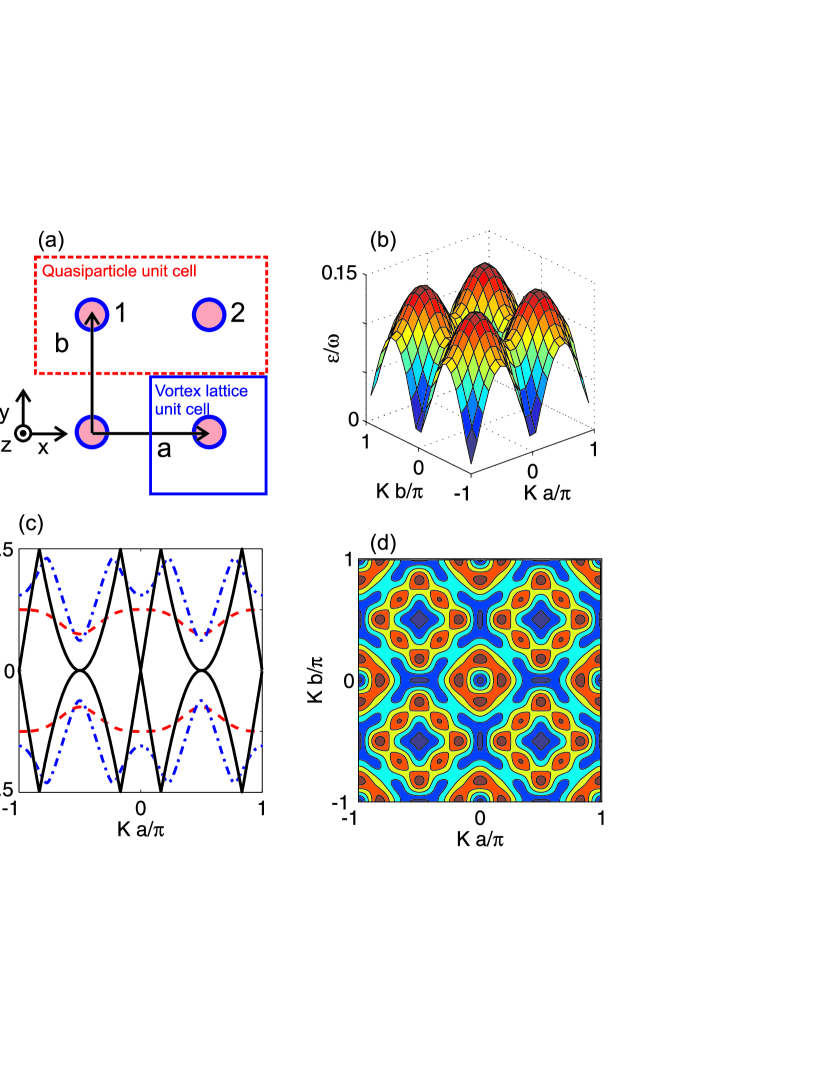
Figure 1: (a) The vortex lattice unit cell and corresponding quasiparticle unite cell containing the nodes marked by 1 and 2 in square vortex lattice. The vortex positions are marked with red filled circles which form the 2D Brave lattice with the basis $({\bf a,b})$. (b) The 3D plot of magnetic Bloch band $\varepsilon_{0+}({\bf K})$ given by (22) $\chi=\pi/4$ and $I_{\bf a}=I_{\bf a}=0.14$. (c) The Bloch bands $\varepsilon_{0\pm}(K_{x},K_{y}=0)$ for $I_{\bf a}=I_{\bf b}=1.4;\;2.8;\;\sqrt{2}\pi$ shown by red dashed, blue dash-dotted and black solid lines correspondingly. (d) The contour plot of $\varepsilon_{0+}({\bf K})$ for $\chi=\pi/4$ and $I_{\bf a}=I_{\bf b}=4.3$. The plots (b,c,d) correspond for the square vortex lattice.

An appealing possibility offered by the nontrivial structure of fermionic spectrum in the vortex phase of chiral $p_{x}+ip_{y}$ superconductors is the realization of quantum matter with exotic non-Abelian quasiparticle statistics SternNature ; IvanovPRL . In this case the non-Abelian anyons are presented by vortex excitations supporting zero-energy Majorana fermions residing inside their cores. That is the spectrum of vortex core fermions is given by

$$\varepsilon=\omega(n+\gamma)$$ (1)

where $n$ is integer number, $\gamma=1/2$ for $s$ wave CdGM and $\gamma=0$ for $p_{x}+ip_{y}$ wave VolovikPwave superconductors. Thus in topologically non-trivial superconductors the spectrum of vortex core fermions (1) contains zero-energy modes with $n=0$ which can be conveniently described in terms of Majorana self-conjugated fermionic fieldIvanovPRL . The ground state of the system with multiple spatially well separated vortices with zero bound fermionic modes is topologically degenerate. The non-Abelyan statistics of vortex anyons allows for the unitary transformations of the ground state realized through the adiabatic permutation of vortices. Such possibility provides an extra motivation for the study of vortices in $p_{x}+ip_{y}$ superconductors due to their potential application in topological quantum computing TQCrmp .

Vortex core Majorana fermions have an important property of being stable with respect to the impurity scatteringVolovikPwave and order parameter perturbations IvanovPRL . However the spectrum vortex core states is extremely sensitive to the intervortex quasiparticle tunnelling. The corresponding spectrum modification in finite clusters of vortices was investigated first by Mel’nikov and Silaev MS1 ; MS2 . In particular for the generic problem of two vortices placed at the distance $d$ the low energy fermionic spectrum has the form

$$\varepsilon=\frac{\omega}{\pi}\left[\pm\arccos(\sqrt{1-e^{-\alpha}}\sin\beta)+\pi(n+1/2+\gamma)\right]\,$$ (2)

where $\gamma=1/2$ for $s$ wave and $\gamma=0$ for $p_{x}+ip_{y}$ wave superconductivity, $\alpha=2\pi e^{-2d/\xi}k_{F}\xi^{2}/d$, $\beta=k_{F}d+\alpha\ln(k_{F}\xi^{2}/d)+\arg(\Gamma(1-i\alpha))+\pi/4$ where $\Gamma(x)$ is Gamma function. The spectrum (2) contains two series of levels with the interlevel distance $\omega\simeq\Delta_{0}/(k_{F}\xi)$, where $\Delta_{0}$ is the gap value far from the vortex core, $\xi$ is the superconducting coherence length. The Eq.(2) demonstrates that the perturbation of energy levels due to the intervortex quasiparticle tunnelling in general is not described by the plain tight binding theory. Indeed the shift of energy levels with respect to the isolated vortex spectrum becomes larger than the energy level spacing $\omega$ when the intervortex distance is smaller than the critical one $d<d_{c}$, where $d_{c}\simeq(\xi/2)\ln(k_{F}\xi)$ is much larger then $\xi$ since $k_{F}\xi\gg 1$. For the typical parameter $k_{F}\xi=100$ corresponds to magnetic fields being larger than that of the order $0.1H_{c2}$.

Thus in a pair of vortices the intervortex quasiparticle tunnelling removes the twofold degeneracy of vortex core states. In particular in $p_{x}+ip_{y}$ superconductor it splits the Majorana zero energy states provided the phase $\beta\neq\pi n$ in the Eq.(2). Such splitting of zero energy levels opens the gap in the fermionic spectrum and can break the quantum coherence during the vortex permutation which is important for the fault tolerance of topological quantum computations Galitskii . The generalization of Eq.(2) for $M-$ vortex clusters is straightforward and was discussed in detailMS1 ; MS2 . In particular for an odd number of vortices $M$ there is always at least one zero energy state irrespective of the vortex position in the cluster. Thus the splitting of Majorana fermions in vortex cluster is not a generic effect and depends on the parity of the total number of vortices $M$. On the other hand in clean type-II superconductors without disorder and pinning centers vortices in finite magnetic field form periodic Abrikosov flux lattice. Therefore the natural question considered in the present paper is whether the spectrum of fermions on the vortex lattice in chiral $p_{x}+ip_{y}$ superconductor is gapped or contains zero energy Majorana states.

Previously the various types of two dimensional lattice spectrum problems of Majorana fermions were considered Kitaev ; Laumann ; SternSquare ; SternNJP ; Lahtinen . These models take into account only the tunnelling between lowest energy states in the vortex cores. As we have discussed above in the generic problem of two vortices the shift of vortex core energy levels becomes larger than the interlevel energy already at small magnetic fields $H\geq 0.1H_{c2}$. Therefore the one level approximation of lattice models is applicable for sparse vortex lattices. Instead in the present paper we consider the eigenvalue problem of genuine Bogolubov - de Gennes equation in chiral $p_{x}+ip_{y}$ superconductor with gap potential corresponding to the periodic Abrikosov flux lattice. To treat this problem we generalize the original approach developed earlier MS1 ; MS2 to calculate the fermionic spectra of finite vortex clusters. This approach allows to calculate the spectrum when the intervortex distance is $d\geq\xi$.

In general the problem of identifying the quasiparticle energies in superconductors is to solve the Bogolubov - de Gennes (BdG) equations having the form:

$$\hat{H}_{0}\Psi+\left(0\quad\;\,\hat{\Delta}\atop\hat{\Delta}^{+}\quad 0\right)\Psi=\varepsilon\Psi\ ,$$ (3)

where $\hat{H}_{0}=\hat{\tau}_{3}\left[(\hat{\bf p}-\hat{\tau}_{3}{\bf A})^{2}-k_{F}^{2}\right]/2m$, $\Psi=(U,V)$, $U$ and $V$ are the particle- and hole - like parts of the fermionic quasiparticle wave function, $\hat{\sigma}_{i}$ are Pauli matrices, $\hat{\bf p}=-i\nabla$, $\hat{\tau}_{i}$ are the Pauli matrices in a particle–hole space, the gap operator is $\hat{\Delta}=\left\{\Delta(\hat{\bf{r}}),e^{i\chi\theta_{p}}\right\}$ where $\chi=\pm 1$ is chirality, $\hat{\bf{r}}$ is a coordinate operator, $\Delta({\bf{r}})$ describes the spatial dependence of the gap function and $\{A,B\}=(AB+BA)/2$ is an anticommutator which provides the gauge invariance of $\hat{\Delta}$. The phase of the order parameter depends on the direction of the electron momentum in $xy$ plane: ${\bf p}=p(\cos\theta_{p},\sin\theta_{p})$. The magnetic field is directed along the $z$ axis ${\bf B}=B{\bf z}$ and for extreme type-II superconductors we can consider the magnetic field to be homogeneous on the spatial scale of intervortex distance and take the gauge ${\bf A}=[{\bf B}\times{\bf r}]/2$ where ${\bf B}$ is an average magnetic field.

Then the periodicity of vortex lattice is determined

$$\Delta({\bf r+d})=e^{i{[\bf B\times d]r}+i\varphi_{\bf d}}\Delta({\bf r})$$ (4)

$${\bf A}({\bf r+d})={\bf A}({\bf r})+[{\bf B}\times{\bf d}]/2$$ (5)

where ${\bf d}=n_{a}{\bf a}+n_{b}{\bf b}$ is the translation of the vortex lattice, $n_{a},n_{b}$ are integer numbers and $\varphi_{\bf d}$ is an arbitrary constant phase shift. By choosing the Wigner-Seitz elementary cell of vortex lattice and placing the origin ${\bf r}=0$ at the vortex center in this cell we immediately obtain that $\varphi_{\bf a}=\varphi_{\bf b}=\pi$.

The translational properties of $\Delta({\bf r})$ and ${\bf A}({\bf r})$ make the Eq.(3) to commute with the magnetic translation operator

$$T^{h}_{{\bf d}}=\hat{\tau}_{3}e^{i\hat{\tau}_{3}{[\bf B\times d]r}/2}T_{{\bf d}}$$ (6)

so that $T^{h}_{{\bf d}}\hat{H}T^{h+}_{{\bf d}}=\hat{H}$ where $T_{{\bf d}}$ is the usual translation by the lattice vector ${\bf d}$. Consequently the solutions of the BdG Eq.(3) can be classified according to the eigenstates of magnetic translation operator. An important point is that the magnetic flux through the vortex lattice unit cell is one half of the flux quantum $B{\bf z}\cdot[{\bf a\times\bf b}]=\pi$ so that the magnetic translations by lattice vectors anticommute $T^{h}_{{\bf a}}T^{h}_{{\bf b}}=-T^{h}_{{\bf b}}T^{h}_{{\bf a}}$. Therefore we should introduce the unit cell for the quasiparticle functions consisting of two vortex lattice unit cells, for example shifted by the vector ${\bf a}$. For the case of square vortex lattice this choice is illustrated in the Fig.1(a). Then the magnetic translation subgroup is formed by vectors ${\bf d_{m}}=2n_{a}{\bf a}+n_{b}{\bf b}$ and the solution of Eq.(3) in general has the form

$$\Psi=\sum_{\bf d_{m}}e^{i{\bf Kd_{m}}}T^{h}_{{\bf d_{m}}}\left[\Psi_{1}({\bf r})+e^{i{\bf Ka}}\Psi_{2}({\bf r})\right]$$ (7)

where the functions $\Psi_{1,2}({\bf r})$ are localized in the centers of vortices forming the unit lattice cell for the quasiparticles (see Fig.1). We substitute the ansatz (7) to the BdG Eq.(3) and calculate the inner product with $\Psi_{1,2}({\bf r})$ taking into account only overlap with neighbor cites to obtain the system of tight binding equations.

The further calculation requires expansion of the node wave functions $\Psi_{1,2}({\bf r})$ by the basis of localized fermionic states of an isolated vortex. It can be implemented using the quasiclassical approximation and the convenient formalismMS1 ; MS2 of the so called $s-\theta_{p}$ representation which allows to express the quasiparticle wave function in momentum representation in the form:

$$\Psi({\bf p})=\frac{1}{k_{F}}\int\limits_{-\infty}^{+\infty}dse^{-i(|{\bf p}|-k_{F})s/\hbar}\psi(s,\theta_{p})\ .$$ (8)

The equation for $\psi(s,\theta_{p})$ reads: $\hat{H}\psi=E\psi$, where

$$\hat{H}=-iV_{F}\hat{\tau}_{3}\partial_{s}+\left(0\quad\;\,\hat{\Delta}\atop\hat{\Delta}^{+}\quad 0\right)\ ,$$ (9)

$V_{F}=k_{F}/m$ is Fermi velocity. Here we take into account the quantization of angular motion variable by treating the angular momentum as differential operator $\hat{\mu}=-i\partial/\partial\theta_{p}$. Hence the spatial coordinate in the gap operator in Eq.(9) is quantum variable in $s-\theta_{p}$ representation $\hat{\bf r}=s{\bf k}_{F}/k_{F}+\left\{[{\bf k}_{F},{\bf z}],\hat{\mu}\right\}/k_{F}^{2}$. Let us emphasize that the Hamiltonian (9) takes account of noncommutability of $\hat{\mu}$ and $\theta_{p}$ and, thus, the above description involves the angular momentum quantization. Replacing $\hat{\mu}$ by a classical variable we get Andreev equations along straight trajectories. The inner product can be expressed through the envelope functions

$$\langle\Psi_{1}|\Psi_{2}\rangle=\frac{\pi}{k_{F}}\int_{-\infty}^{\infty}ds\int_{0}^{2\pi}d\theta_{p}\psi^{+}_{1}\psi_{2}(s,\theta_{p})$$ (10)

and the magnetic translation operator (6) in $s-\theta_{p}$ representation has the form $T^{h}_{\bf d}=\hat{\tau}_{3}e^{-i\varphi_{h}({\bf d})\hat{\tau}_{3}/2}T_{\bf d}$ where $\varphi_{h}({\bf d})=d(s+{\bf nd})\sin(\theta_{p}-\theta_{d})$, the angle $\theta_{d}$ defines the direction of ${\bf d}=d(\cos\theta_{d},\sin\theta_{d})$ and $T_{\bf d}=\exp\left[-i{\bf dk_{F}}(1-ik_{F}^{-1}\partial_{s})\right]$ is the translation operatorMS1 .

The form of the node functions $\Psi_{1,2}(\bf r)$ in Eq.(7) is determined by the states localized in isolated vortex. We consider the vortex lattice cite $1$ centered at the origin ${\bf r}=0$ and define the spatial dependence of gap function inside the unit cell as $\Delta({\bf r})=\Delta_{v}(r)e^{i\theta}$ where $\Delta_{v}(r=0)=0$. Then eigenfunctions of the Hamiltonian (9) centered at lattice cites $1$ and $2$ have the form

$$\psi_{1}(s,\theta_{p})=C_{1}(\theta_{p})\psi_{v}(s,\theta_{p})$$ (11)

$$\psi_{2}(s,\theta_{p})=C_{2}(\theta_{p})T^{h}_{\bf a}\psi_{v}(s,\theta_{p})$$ (12)

where ${\bf n}={\bf k_{F}}/k_{F}$ and

$$\psi_{v}(s,\theta_{p})=e^{i\hat{\tau}_{3}(1+\chi)\theta_{p}/2}\left(1\atop-i\right)\frac{e^{-K(s)}}{\sqrt{\Lambda}},$$ (13)

$K(s)=V_{F}^{-1}\left|\int\limits_{0}^{s}\Delta_{v}(t)dt\right|$ and $\Lambda$ is normalizing factor so that $\langle\Psi|\Psi\rangle=1$ . The node functions are translated to other sides according to the Eq.(6) so that with the help of Eq.(10) we obtain the inner products, e.g.

$$\langle\Psi_{j}|\hat{H}|\Psi_{j}\rangle=\omega\int_{0}^{2\pi}C^{*}_{j}\hat{\mu}C_{j}\frac{d\theta_{p}}{2\pi}$$ (14)

$$\langle\Psi_{j}|\hat{H}|T^{h}_{\bf b}\Psi_{j}\rangle=i(-1)^{j+1}J_{\bf b}\int_{0}^{2\pi}e^{-i{\bf bk_{F}}}C^{*}_{j}C_{j},$$ (15)

$j=1,2$ where ${\bf d=a,b}$ and the Hamiltonian $\hat{H}$ is given by (9). The sign in Eq.(15) determined by the magnetic flux through the unit cell. Here for simplicity we take into account the overlap with four neighboring vortices. The cases of more neighbors can be considered analogously. The main contribution to the inner products of the form (15) comes from the stationary points of the phases $({\bf ak_{F}})$ and $({\bf bk_{F}})$ that is $\theta_{p}^{*}=\theta_{a,b}+\pi n$. The stationary points $\theta_{p}^{*}$ correspond to the trajectories passing through both of the neighbor vortex cores which means that we can calculate the overlap factors as follows

$$J_{\bf d}=\frac{\pi}{k_{F}}\int_{-\infty}^{\infty}\left[\Delta(s)-\tilde{\Delta}_{v}(s_{1})\right]\tilde{\psi}_{v}^{+}(s)\hat{\tau}_{2}\tilde{\psi}_{v}(s_{1})ds.$$ (16)

where $s_{1}=s-{\bf nd}$, $\tilde{\Delta}_{v}(s)=\Delta_{v}(s)sign(s)$, and $\tilde{\psi}_{v}(s)=\psi_{v}(s,\theta_{p}=0)$. Then with good accuracy Eq.(16) yields an estimation $\left|J_{\bf d}\right|\approx\Delta_{0}\exp\left(-d/\xi\right)$.

With the help of the inner products (14,15) and taking into account that $J_{\bf d}=-J_{-\bf d}$ we obtain the equations

$$(\varepsilon-\omega\hat{\mu})C_{1}=F_{\bf b}(\theta_{p})C_{1}+F_{\bf a}(\theta_{p})C_{2}$$ (17)

$$(\varepsilon-\omega\hat{\mu})C_{2}=-F_{\bf b}(\theta_{p})C_{2}+F_{\bf a}(\theta_{p})C_{1}$$

where $F_{\bf d}(\theta_{p})=J_{\bf d}\sin[{\bf d}({\bf k_{F}+K})]$ and ${\bf d}={\bf a,b}$. The system (17) should be solved together with periodic boundary conditions $C_{1,2}(\theta_{p})=C_{1,2}(\theta_{p}+2\pi)$ for $p_{x}+ip_{y}$ wave and $C_{1,2}(\theta_{p})=C_{1,2}(\theta_{p}+2\pi)$ for $s$ wave. Note that in Eqs.(17) we can take into account overlapping with next-to neighbor vortices which will introduce the corrections of the relative order $e^{-d/\xi}$ to the coefficients $F_{\bf a,b}$. Here we neglect such corrections.

To solve the Eq.(17) we use the approximate method employed earlier for the system of two vorticesMS1 . That is besides the vicinity of the angles $\theta_{p}^{*}=\theta_{a,b}+\pi n$ the solution with good accuracy is $C_{1,2}\sim e^{i\varepsilon\theta_{p}/\omega}$. In the $\delta$ vicinity of the angles $\theta_{p}^{*}$ the system (17) diagonalizes yielding the matching conditions ${\bf C}(\theta_{p}^{*}+\delta)=\hat{M}{\bf C}(\theta_{p}^{*}-\delta)$ for the vector ${\bf C}=(C_{1},C_{2})^{T}$. The matching matrices are

$$\hat{M} (\theta_{b})=\exp(-i\hat{\tau}_{3}\chi_{b+})$$ (18)

$$\hat{M} (\theta_{b}+\pi)=\exp(-i\hat{\tau}_{3}\chi_{b-})$$ (19)

$$\hat{M} (\theta_{a})=\cos\chi_{a+}-i\hat{\tau}_{1}\sin\chi_{a+}$$ (20)

$$\hat{M} (\theta_{a}+\pi)=\cos\chi_{a-}-i\hat{\tau}_{1}\sin\chi_{a-}$$ (21)

where $\chi_{d\pm}=I_{\bf d}\sin({\bf Kd}\pm\chi)$ where $\chi=k_{F}d-\pi/4$ and $I_{{\bf d}}=(J_{\bf d}/\omega)\sqrt{\pi/k_{F}d}$.

The periodic boundary condition and Eqs.(18) yield the Bloch waves $\varepsilon=\varepsilon_{n}({\bf K})$ in a periodic Abrikosov flux lattice

$$\varepsilon_{n\pm}({\bf K})=\omega\left(\pm\frac{\arccos X}{2\pi}+n+\gamma\right)$$ (22)

where $\gamma=1/2$ for $s$ wave and $\gamma=0$ for $p_{x}+ip_{y}$ wave, $X=\cos\chi_{a-}\cos\chi_{a+}\cos(\chi_{b+}+\chi_{b-})-\sin\chi_{a-}\sin\chi_{a+}\cos(\chi_{b+}-\chi_{b-})$ and $n$ is integer. The width of Bloch bands (22) is determined by the overall amplitude $max(\omega,\Delta_{0}e^{-d/\xi}/\sqrt{k_{F}d})$ and rapid oscillations with the period $k^{-1}_{F}$ by the intervortex distances $a,b$. The phase of oscillations is determined by the average magnetic field, e.g. $a=b=\sqrt{\Phi_{0}/B}$ for the square lattice where $\Phi_{0}$ is magnetic flux quantum for Cooper pairs. Notwithstanding the rapid oscillations of the bandwidth the spectrum (22) survives fluctuations of the vortex positions ${\bf\delta r}$ provided their amplitude is relatively small. Indeed in case of the disordered vortex lattices let us search the quasiparticle waves in the form $\Psi({\bf r})=\Psi_{0}({\bf r})+\tilde{\Psi}({\bf r})$ where the first term is periodical and given by Eq.(7) and the second term is the distortion due to the fluctuation of vortex positions. We use the expansion (8,11) with the coefficients $\tilde{C}_{1,2},(\theta_{p})$ to represent the distortion $\tilde{\Psi}({\bf r})$ at the particular lattice site. Then we get the equations for $\tilde{C}_{1,2}(\theta_{p})$ $(\varepsilon-\omega\hat{\mu})\tilde{C}_{j}=\omega\tilde{\mu}C_{j0}(\theta_{p})$ where $\tilde{\mu}={\bf z[\delta r\times k_{F}]}$ and $C_{j0}(\theta_{p})$ corresponds to the periodical part of function $\Psi_{0}({\bf r})$ determined by the solution of Eq. (17). The functions $C_{j0}(\theta_{p})$ are the rapidly oscillating ones with the characteristic period $\Delta\theta_{p}\approx e^{d/\xi}/(k_{F}\xi)$ so that the amplitude of the distortion is small $\tilde{C}_{j}\sim e^{d/\xi}|\delta{\bf r}|/\xi\ll 1$ provided vortex position fluctuations are small enough $|\delta{\bf r}|\ll\xi e^{-d/\xi}$.

The plot of the Bloch band $\varepsilon_{0+}({\bf K})$ is shown in the Fig.1(b) for the parameters $\chi=\pi/4$ and $I_{\bf a}=I_{\bf b}=0.14$. One can see that this band contains small energy gap. Indeed for $|I_{\bf d}|\ll 1$ the Eq.(22) can be simplified. Taking into account the quadratic terms of the order $I_{\bf d}^{2}$ we obtain the gapless spectrum identical to the one level lattice model SternSquare with the hopping amplitude determined by $\omega|I_{\bf d}|$. On the other hand the terms of the order $I_{\bf d}^{4}$ open the gap in the spectrum which is beyond the accuracy of one level approximation and appear due to the mixing with higher levels. Note that overlap with next-to neighbor vortices introduce correction smaller by the factor $1/\sqrt{k_{F}\xi}$ than the interaction with higher levels. Decreasing the intervortex distance one finally obtains gapless spectrum when $|I_{\bf d}|\geq\pi$. The example of such crossover to the gapless regime is demonstrated in the dependence $\varepsilon(K_{x},K_{y})$ for the square lattice in Fig.1(c). We set $\chi=\pi/4$ and plot by red dash-dotted, blue dashed and black solid lines the Bloch bands $\varepsilon_{0\pm}({\bf K})$ for $I_{\bf a}=I_{\bf a}=1.4;\;2.8;\;\sqrt{2}\pi$ correspondingly. For higher values of the overlap $|I_{\bf d}|$ the structure of Bloch bands becomes more complicated with rapid oscillations as function of quasimomentum with the characteristic period of the order $1/(|I_{\bf d}|d)$. Such complicated structure of Bloch band $\varepsilon_{0+}({\bf K})$ for $\chi=\pi/4$ and $I_{\bf a}=I_{\bf a}=4.3$ is shown in the contour plot Fig.1(d).

Finally let us consider the possible experimental test of the suggested gapless spectrum of Majorana fermions(22).

In addition to the variety of experiments proposed Experiments . the electronic thermal conductivity $\kappa$ measurements have been proven as an effective tool to study the quaiparticle spectrum in the vortex phase Lowell . The electronic states in magnetic Bloch bands (22) can carry the energy current in the direction $\perp{\bf B}$ due to the hopping of quasiparticles between neighboring vortices. The electronic spectrum on Abrikosov lattice (22) is gapless even in the regular lattices provided the intervortex distance is $d<d_{c}$. Hence one should expect the threshold behavior of $\kappa(B)$ in the increasing magnetic field in the limit $T\rightarrow 0$. That is $\kappa$ should be zero in the gapped phase and in the gapless regime it can be estimated by the textbook expression $\kappa_{\perp}\sim TV_{g}^{2}\tau\nu$ where ${\bf V_{g}}=\partial\varepsilon/\partial{\bf K}$ is the group velocity of Bloch waves (22), $\tau$ is transport time and $\nu=\omega^{-1}d^{-2}$ is density of in the vortex lattice. The typical value of group velocity determined by the intervortex hopping is $V_{g}\sim V_{F}e^{-d/\xi}\sqrt{d/k_{F}\xi^{2}}$ so that assuming $d=\beta\xi\sqrt{H_{c2}/B}$ where $\beta\sim 1$ we obtain

$$\kappa_{\perp}/\kappa_{N}=\frac{\sqrt{B/H_{c2}}}{\beta k_{F}\xi}e^{-2\beta\sqrt{H_{c2}/B}}.$$ (23)

Besides that $\kappa_{\perp}$ also contains oscillating part due to rapid oscillations of energy levels (22) with the period $k^{-1}_{F}$ by the intervortex distance. However the oscillations are mostly cancelled out due to the complicated structure of Bloch bands shown in Fig.1(d). The obtained value of $\kappa$ is valid in the superclean limit $\omega\tau>1$ for fully gapped superconductors including $s$ and $p_{x}+ip_{y}$ wave symmetries. The estimation (23) contains small prefactor $1/k_{F}\xi$ which can explain the experimentally observed small values of $\kappa_{\perp}$ at $B\ll H_{c2}$ Lowell . Interestingly the observedExpThCondKes similar to (23) behavior of $\kappa_{\parallel}$ in the direction $\parallel{\bf B}$ can be explained by the theory MS2 applied to the spectrum(22) since the number of conducting modes along vortex line is determined by the tunnelling factors $I_{\bf d}$.

The author thanks Alexander Mel’nikov and Sergei Sharov for many stimulating discussions and Ville Lahtinen for correspondence. The work was supported b y Russian Foundation for Basic Research.

References

- (1) D. J. Thouless, M. Kohmoto, M. P. Nightingale, and M. den Nijs, Phys. Rev. Let. 49, 405 (1982)
- (2) G.E.Volovik, Zh. Eksp. Teor. Fiz. 94, 123 (1988) [English translation: Sov. Phys. JETP 67, 1804 (1988)];. G.E.Volovik, V.M.Yakovenko, J. Phys.: Condens. Matter 1, 5263 (1989).
- (3) A. P. Mackenzie and Y. Maeno Rev. Mod. Phys. 75 657, 2003
- (4) M. A. Silaev and G. E. Volovik Phys. Rev. B 86, 214511 (2012)
- (5) Y. Tsutsumi, M. Ichioka, and K. Machida, Phys. Rev. B 83, 094510 (2011).
- (6) C. Caroli, P. G. de Gennes, J. Matricon, Phys. Lett. 9, 307 (1964).
- (7) G. Volovik, JETP Lett. 70, 609 (1999).
- (8) R.Willett et al., Phys.Rev. Lett. 59, 1776 (1987); W. Pan et al., Phys. Rev. Lett. 83, 3530 (1999).
- (9) L. Fu and C. L. Kane, Phys. Rev. Lett. 100, 096407 (2008).
- (10) J. Chaloupka et al., Phys. Rev. Lett. 105, 027204 (2010); H.-C. Jiang et al., Phys. Rev. B 83, 245104 (2011);
- (11) A. Stern, Nature 464 187 (2010)
- (12) D. A. Ivanov, Phys. Rev. Lett. 86, 268 (2001).
- (13) C. Nayak , A. Simon, A. Stern, A. Freedman and S. Das Sarma Rev. Mod. Phys. 80 1083 (2008)
- (14) A.S.Mel’nikov, M.A.Silaev, JETP Lett. 83 578 (2006)
- (15) A. S. Mel nikov, D. A. Ryzhov, and M. A. Silaev, Phys. Rev. B 78, 064513 (2008)
- (16) Cheng M, Lutchyn R M, Galitski V and Das Sarma S, Phys. Rev. Lett. 103 107001 (2009)
- (17) A. Kitaev, Ann. Phys., 321, 2 (2006)
- (18) C. R. Laumann, A. W. W. Ludwig, D. A. Huse, and S. Trebst Phys. Rev. B, 85, 161301 (2012)
- (19) E. Grosfeld and A. Stern, Phys. Rev. B 73, 201303 (2006)
- (20) Y.E. Kraus and A. Stern, New J. of Phys., 13, 105006 (2011)
- (21) Y. E. Kraus, A. Auerbach, H.A. Fertig and S.H. Simon, Phys. Rev. Lett. 101, 267002 (2008); N.R. Cooper, A. Stern, Phys. Rev. Lett. 102, 176807 (2009); A.R. Akhmerov, J. Nilsson and C. W. J. Beenakker, Phys. Rev. Lett. 102 216404 (2009); L. Fu and C. L. Kane, Phys. Rev. Lett. 102 216403 (2009)
- (22) V. Lahtinen, A. W. W. Ludwig, J. K. Pachos, and S. Trebst, Phys. Rev. B 86, 075115 (2012)
- (23) J.Lowell, J.B. Sousa, J. Low Temp. Phys. 3, 65 (1970)
- (24) P. H. Kes, J. P. M. van der Veeken, and D. de Kierk, J. Low Temp. Phys. 18, 355 (1975).