Adiabaticity and color mixing in tetraquark spectroscopy

Abstract

We revisit the role of color mixing in the quark-model calculation of tetraquark states, and compare simple pairwise potentials to more elaborate string models with three- and four-body forces. We attempt to disentangle the improved dynamics of confinement from the approximations made in the treatment of the internal color degrees of freedom.

I Introduction

There is a persisting interest in the quark dynamics applied to multiquark spectroscopy. The question is whether there exist compact hadron states beyond ordinary mesons (quark–antiquark) and baryons (three quarks).

In simple constituent models, several mechanisms have been proposed for binding multiquarks: chiral dynamics for light quarks, chromomagnetism, clustering of heavy quarks in a chromoelectric potential, etc. In this article, we concentrate on this latter effect, i.e., multiquark binding in a spin- and flavor-independent potential, and discuss the role of the internal color degrees of freedom. The validity of the existing models is beyond the scope of this note. In particular, we shall not discuss the transition from color as a local gauge invariance to color as a global property of the wave-function in constituent models. Still, even in its simplified version, color is a delicate ingredient of multiquark dynamics.

The first studies on multiquarks within constituent models were based on simple color-additive potentials, extrapolated from meson and baryon spectroscopy. Already for baryons, one hardly justifies the choice of a pairwise interaction, half as strong as the quark–antiquark potential, but a more elaborate modeling, based on a connected $Y$-shape flux tube linking the three quarks, does not change the results significantly.

We shall follow in this paper this picture of a minimal string linking the quarks. There are alternative non-trivial pictures of confinement, in particular the ones based on diquarks, which have been extended from the baryon sector to the multiquarks. See, for instance, Maiani:2004vq ; Ebert:2005nc ; Dubnicka:2010kz .

The $Y$-shape potential of baryons has been extended to tetraquarks and higher multiquark configurations Carlson:1991zt . There are multi-$Y$ connected diagrams in which the string interaction links all quarks and antiquarks as a Steiner tree whose cumulated length is minimized. But the dynamics is dominated by the so-called “flip-flop” diagrams, with disconnected flux tubes for each of the quark–antiquark, three-quark or three-antiquark sub-clusters: the attraction comes from the minimum taken over all possible permutations of the quarks and of the antiquarks.

This flip–flop interaction contains 3-body, 4-body, and higher-order terms, and is thus more delicate to handle in variational calculations. Moreover, when two quarks are exchanged, the color wave function is modified. In the latest studies Vijande:2007ix ; Richard:2009rp ; Vijande:2011im , this effect is not treated rigorously. Instead, a type of adiabatic approximation is used: for any set of coordinates for the quarks, the potential is taken as the minimum of all permutations of the quarks and antiquarks, irrespective of the color wave function, and this minimum, as a function of the coordinates, is interpreted as an effective potential leading to a few-body spectral problem in which color has disappeared. Interestingly, this strategy leads to stable multiquarks for a large variety of constituent masses. This is at variance with the color-additive model, which binds only tetraquarks for large values of the quark-to-antiquark mass ratio.

The question is thus whether the multiquark binding obtained in string models survives a non-adiabatic treatment of the internal color degrees of freedom. The problem is analyzed in the present paper by reformulating the string-based interaction as an operator in color space.

The outline is the following. In Sec. II, we set the notation for the color components of tetraquarks. In Sec. III, we present various models of tetraquark confinement with coupled channels in color space or an adiabatic approximation in which color disappears from the final wave-equation. The results are presented in Sec. IV, and the conclusions in Sec.V.

II Color states

The internal color structure of tetraquark states is described in several papers, see, e.g. Chan:1977st ; Chan:1978nk ; Vijande:2009ac . We shall borrow the notation of Chan:1977st , in particular the names “true baryonium” ($T$) and “mock baryonium” ($M$), though the physics context is rather different in the present heavy-quark spectroscopy as compared to the color chemistry of the late 70s.

The wave function for $(1,2,3,4)=(qq\bar{q}\bar{q})$ is written as

$$\Psi=\psi_{T}\,|T\rangle+\psi_{M}\,|M\rangle$$ (1)

where $|T\rangle$ denotes a color state with the two quarks in a color $\bar{3}$ state, and the antiquarks in a color 3, while $|M\rangle$ corresponds to a color sextet in the quark sector and antisextet in the antiquark one. There is also the possibility of building the global color state out of quark–antiquark clusters either in a color singlet or octet. More precisely, we introduce

$$|T\rangle =|(12)_{\bar{3}}\,(34)_{3}\rangle~{},\quad |M\rangle =|(12)_{6}\,(34)_{\bar{6}}\rangle~{},$$ (2)

$$|1\phantom{{}^{\prime}}\rangle =|(13)_{1}\,(24)_{1}\rangle~{},\quad |8\phantom{{}^{\prime}}\rangle =|(13)_{8}\,(24)_{8}\rangle~{},$$

$$|1^{\prime}\rangle =|(14)_{1}\,(23)_{1}\rangle~{},\quad |8^{\prime}\rangle =|(14)_{8}\,(23)_{8}\rangle~{}.$$

The relations between the different sets can be deduced from

$$|1\phantom{{}^{\prime}}\rangle =\phantom{+}\sqrt{\frac{1}{3}}\,|T\rangle+\sqrt{\frac{2}{3}}\,|M\rangle~{},$$ (3)

$$|8\phantom{{}^{\prime}}\rangle =-\sqrt{\frac{2}{3}}\,|T\rangle+\sqrt{\frac{1}{3}}\,|M\rangle~{},$$

$$|1^{\prime}\rangle =-\sqrt{\frac{1}{3}}\,|T\rangle+\sqrt{\frac{2}{3}}\,|M\rangle~{},$$

$$|8^{\prime}\rangle =\phantom{+}\sqrt{\frac{2}{3}}\,|T\rangle+\sqrt{\frac{1}{3}}\,|M\rangle~{}.$$

Accordingly, the matrix elements of the potential in any basis are related to the ones in another basis, for instance,

$$V_{11}=\langle 1|V|1\rangle=\frac{1}{3}\,V_{TT}+\frac{2}{3}\,V_{MM}+\frac{2\,\sqrt{2}}{3}\,V_{TM}~{},$$ (4)

and many similar relations.

As stressed by Lipkin Lipkin:1986dw , in the limit of a tetraquark with two units of heavy flavor, $(QQ\bar{q}\bar{q})$ with a large quark-to antiquark mass ratio $M/m$, the ground state is an almost pure $|T\rangle$ state, with the two flavored quarks in an antitriplet state, as in ordinary $(QQq)$ baryons, and the two antiquarks neutralizing that color, as in $(\bar{Q}\bar{q}\bar{q})$ antibaryons. In other words, the tetraquark state in the large $M/m$ limit just uses well probed color structures, such as the $3\otimes 3\to\bar{3}$ coupling of two quarks in baryons.

On the other hand, for smaller values of the mass ratio $M/m$, the simple models give at best a very shallow binding. Then the mixing of $|T\rangle$ and $|M\rangle$ is crucial to establish the stability. See, e.g., Brink and Stancu Brink:1994ic .

III Models of tetraquark confinement

In early days of multiquark calculations, the potential was assumed to be pairwise, with the color dependence associated with the exchange of a color octet, namely

$$V=-\frac{3}{16}\,\sum_{i<j}\tilde{\lambda}_{i}.\tilde{\lambda}_{j}\,v(r_{ij})~{}.$$ (5)

Here, $\tilde{\lambda}_{i}$ is the color operator for the $i^{\text{th}}$ quark, and is suitably modified for an antiquark belonging to the $\bar{3}$ representation of SU(3). The normalization is such that $v(r_{ij})$ is the central part of the quarkonium potential.

This model, however crude, gives at least the possibility of studying the role of the internal color degrees of freedom inside a multiquark state.

The additive model being subject to heavy criticism, an alternative was sought, inspired by the strong-coupling regime of QCD. It is referred to as the flip–flop model. For mesons, the potential is $V=\sigma\,r$, where $r$ is the quark–antiquark distance, and $\sigma$ the string tension, which can be set to $\sigma=1$ by rescaling, without loss of generality. For baryons, this is the $Y$-shape interaction $V_{Y}=\min_{a}(r_{1a}+r_{2a}+r_{3a})$. For a tetraquark, the potential is the minimum of the flip–flop term and a connected string, namely Carlson:1991zt ; Vijande:2007ix

$$V_{4} =\min(V_{\text{ff}},V_{\text{s}})~{},$$ (6)

$$V_{\text{ff}} =\min(r_{13}+r_{24},r_{14}+r_{23})~{},$$

$$V_{\text{s}} =\min_{a,b}(r_{1a}+r_{2a}+r_{ab}+r_{3b}+r_{4b})~{},$$

as pictured in Figs. 1.

     

Figure 1: Top: schematic picture of the quark–antiquark and three-quark confinement. Bottom: three contributions to the tetraquark potential; the simple string model takes the minimum of these three contributions

For each set of quark coordinates $\boldsymbol{r}_{i}$, the minimization in (6) implies a rotation in color space. This means that $V_{4}$ is an adiabatic approximation, which tends to overbind the system. More importantly, the minimization, at least as it was carried out in Vijande:2007ix , does not account for any antisymmetrization. It just holds for distinguishable quarks or antiquarks.

As the model (6) gives an interesting spectrum of stable tetraquarks Vijande:2007ix , and, if extended to higher configurations, a spectrum of bound pentaquarks and hexaquarks Richard:2009rp ; Vijande:2011im , it is crucial to estimate the amount of overbinding due to the adiabatic approximation, and the changes occurring when a proper antisymmetrization is implemented.

We aim at constructing an operator in color space that tends to (6) in the adiabatic limit, at least when one of the three terms is clearly the minimum. For instance, if the (1,3) pair is clustered and lies far from the (2,4) pair which is also clustered, the potential is more easily described in the $\{|1\rangle,\,|8\rangle\}$ basis. However, working solely in this latter basis would require the choice of a value for the string tension between color-octet objects (there are studies within QCD, see, e.g., Bali:2000un ) and an ansatz for the transition potential $V_{18}$. Instead, we shall combine the pieces of information coming from the singlet–singlet and triplet–antitriplet states, to deduce the full $2\times 2$ matrix of the potential in the $\{|T\rangle,\,|M\rangle\}$ basis, in which the four-body problem will be solved.

More precisely, we will consider four different models:

• Model A is the adiabatic limit given by (6), already used in Vijande:2007ix . However, the Steiner-tree with two junctions, that plays a marginal role, is neglected. Hence, this is the pure flip–flop model.

• Model B is a smooth version of the adiabatic approximation. We use $g(x)=1/(1+x^{n})$ and its complement $g^{\prime}(x)=1-g(x)$, with some large but finite exponent $n=5$ to soften the transition between different limiting regimes of the string model. In practice, we replace the above $V_{TT}$ by

  $$\hat{V}_{TT}=g_{3}\,g^{\prime}_{3}\,V_{TT}+(1-g_{3}\,g^{\prime}_{3})\\ {}\times\Biggl{[}\frac{3\,V_{1^{\prime}1^{\prime}}+V_{11}}{4}\,g_{1}{}+\frac{3\,V_{11}+V_{1^{\prime}1^{\prime}}}{4}\,g^{\prime}_{1}\Biggr{]}~{},$$ (7)

  where

  $$V_{11}=r_{13}+r_{24}~{},\quad V_{1^{\prime}1^{\prime}}=r_{14}+r_{23}~{},$$ (8)

  and

  $$g_{3} =g\left(\frac{V_{33}}{V_{11}}\right)~{},\quad g^{\prime}_{3}=g\left(\frac{V_{33}}{V_{1^{\prime}1^{\prime}}}\right)~{},$$ (9)

  $$g_{1} =1-g^{\prime}_{1}=g\left(\frac{V_{11}}{V_{1^{\prime}1^{\prime}}}\right)~{}.$$

  Then, the potential is known in any basis from $V_{11}$, $V_{1^{\prime}1^{\prime}}$ and $\hat{V}_{TT}$. For instance, in the $\{|1\rangle,\,|8\rangle\}$ basis, one uses $V_{11}$ and

  $$V_{18} =\frac{1}{4\sqrt{2}}\{V_{11}+3V_{1^{\prime}1^{\prime}}-4\hat{V}_{TT}\}$$ (10)

  $$V_{88} =\frac{1}{4}\{-V_{11}+3V_{1^{\prime}1^{\prime}}+2\hat{V}_{TT}\}~{},$$

  and it is readily checked that if $g_{1}\to 1$, the potential becomes diagonal. The four-body problem is more conveniently solved in the $\{|T\rangle,\,|M\rangle\}$ basis, and besides $\hat{V}_{TT}$, the relevant matrix elements are

  $$V_{TM} =\frac{3}{4\sqrt{2}}\{V_{11}-V_{1^{\prime}1^{\prime}}\}$$ (11)

  $$V_{MM} =\frac{1}{4}\{3V_{11}+3V_{1^{\prime}1^{\prime}}-2\hat{V}_{TT}\}~{},$$

• Model C is the color-additive model of (5), normalized to a unit string tension for quarkonium.

• Model D is the crude adiabatic limit of the previous one. This means that for any given set of positions, the $2\times 2$ matrix consisting of $V_{TT}$, $V_{TM}$ and $V_{MM}$ of model 4 is diagonalized, and the lowest eigenvalue is taken as the effective four-body potential, irrespective of any symmetrization or antisymmetrization. Of course, model D is more attractive than model C.

• Several other variants have been envisaged, but abandoned as leading to collapses or inconsistencies. For instance, it is tempting to use relations similar to (11) to express $V_{TM}$ and $V_{MM}$ from $V_{11}$, $V_{1^{\prime}1^{\prime}}$ and $V_{TT}$, as given by the string model. But then the Hamiltonian is not bounded below.

IV Results

The results are shown in Table 1. The aim is not to provide a benchmark of four-body calculations. What really matters, is how the ground-state energy evolves when going from a model to another one. The variational estimate has been carried out using just a few Gaussians, and in the case of models B and C, imposing the proper symmetry.

For this purpose, we make use of a wave function with the relevant symmetry for each color component. As the color vector $|T\rangle$ ($|M\rangle$) is antisymmetric (symmetric) under both the exchange of the identical quarks and the identical antiquarks, it has to be combined with a radial wave function with the proper symmetries. The way of constructing these wave functions has been explicitly detailed in Ref. Vijande:2009ac . We will just draft here its main characteristics. The radial wave function is taken as a linear combination of generalized Gaussians depending on six variational parameters $a_{ij}$ of the form,

$$\Psi(\boldsymbol{x_{1}},\boldsymbol{x_{2}},\boldsymbol{x_{3}})=\sum_{k=1}^{4}\alpha_{k}\exp\left[-\sum_{i\geq j=1}^{3}a_{ij}s_{ij}^{k}\,\boldsymbol{x}_{i}\cdot\boldsymbol{x}_{j}\right],$$ (12)

where $s^{k}$ are six-component $(ij)$ vectors made of arrangements of positive and negative signs. Once combined with the proper election of the signs $\alpha_{k}$, they give rise to radial wave functions with the following symmetries in the radial space under the exchange of quarks and antiquarks: $SS,SA,AS,$ or $AA$, where $S$ stands for symmetric and $A$ for antisymmetric.

Table 1: Results for the various models A, B, C and D, as a function of the quark-to-antiquark mass ratio $M/m$

$M/m$	A	B	C	D	Threshold
1.	4.644	4.803	4.702	4.596	4.676
2.	4.211	4.306	4.275	4.160	4.248
3.	4.037	4.131	4.112	3.984	4.086
4.	3.941	4.041	4.010	3.891	3.998
5.	3.880	3.985	3.954	3.828	3.942
10.	3.742	3.860	3.834	3.685	3.831

The results from models A and D are very similar for the variational energies. This means that the extra attraction noticed in Vijande:2007ix is mainly due to the color mixing in the adiabatic approximation. Restoring the interaction as an operator in color space is less favorable for multiquark binding, and it is readily seen that models B and C led to comparable predictions. The color structure of the wave-functions is also rather similar in models B and C, with mostly a singlet–singlet configuration.

However, if one looks at the details, it can be realized that the flip–flop and and the additive models differ. In particular, the average $QQ$ separation, $\langle r_{12}\rangle$ is smaller in the additive model than in the flip–flop model. If the mass ratio $M/m\to\infty$, this effect becomes more pronounced, with $\langle r_{12}\rangle\to 0$ in the former case and $\langle r_{12}\rangle$ evolving to a finite value (for $m$ fixed) in the latter one. This influences the contribution of the $W$-exchange contribution to the weak decay of $(bc\bar{q}\bar{q})$, which also plays a role in the decay of $(bcu)$ baryons Korner:1994nh .

This large $M/m$ limit is rather interesting. A detailed numerical study would involve the computation of an effective $QQ$ interaction, $V_{\text{eff}}(r_{12})$, sum of the direct $QQ$ interaction and of the $\bar{q}\bar{q}$ binding energy around them, very similar to the Heitler–London potential of two protons in the adiabatic treatment of the hydrogen molecule. Already, for baryons with two heavy quarks, $(QQq)$, it was stressed that the Born–Oppenheimer approximation works very well to reproduce the properties of the lowest states Fleck:1989mb . For $(QQ\bar{q}\bar{q})$, it is striking that the effective potentials $V_{\text{eff}}(r_{12})$ have qualitative differences in the additive model and in the flip–flop one. In the additive model, the minimum of $V_{\text{eff}}(r_{12})$ is reached at $r_{12}=0.$ The $\bar{q}\bar{q}$ contribution is stationary there. So, up to a constant, the potential is dominated by the direct $QQ$ term, which is $r_{12}/2$ here. Thus the average separation decreases as $M^{-1/3}$, according to the well-known scaling laws in a linear potential Quigg:1979vr . In the flip–flop model, $V_{\text{eff}}(r_{12})$ is minimum at some finite distance. This can be seen directly. This is also compulsory, if one wishes to understand why $(QQ\bar{q}\bar{q})$ is stable in the large $M/m$ limit, as seen by the following reductio ad absurdum: suppose that in the Born–Oppenheimer limit of the flip–flop model, $\langle r_{12}\rangle\to 0$, then the flip–flop energy of $(QQ\bar{q}\bar{q})$ and the energy of its threshold, $(Q\bar{q})+(Q\bar{q})$, which are pictured in Fig. 2 and given by

$$V_{\text{eff}}(r_{12}) =\min(r_{13}+r_{24},r_{14}+r_{23})~{},$$ (13)

$$V_{\text{th}} =r_{13}+r_{24}~{},$$

would coincide if $r_{12}=0$ and the inequality among energies $(QQ\bar{q}\bar{q})<(Q\bar{q})+(Q\bar{q})$ would be impossible.

Figure 2: Flip-flop potential for $r_{12}\to 0$ and cumulated potential of two mesons

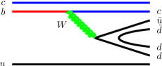
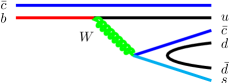
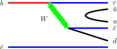
Figure 3: Some weak decays of the $(bcu)$ baryon and $(b\bar{c})$ meson leading to a tetraquark in the final state

V Conclusions

Our results illustrate the role of antisymmetrization in preventing from a proliferation of multiquarks. In particular, the main difference between the naive color-additive model and the crude flip–flop model comes from the treatment of color. It remains that in such a flavor-independent confining, the binding of $(QQ\bar{q}\bar{q})$ is obtained for heavy enough quarks.

More ambitious tools are obviously needed to handle the four-quark dynamics. In particular, in the double-charm sector, the binding effect of the confining interaction is probably not sufficient. In addition, the spin-part of the wave function can be made favorable: as stressed, e.g., in Hyodo:2012pm and references therein, there is a light–light interaction in $(cc\bar{u}\bar{d})$ which is absent in the two mesons constituting the threshold.

The production of such tetraquarks can be accessible in B-factories Hyodo:2012pm and at the proton–proton colliders. Note also that $(cc\bar{q}\bar{q})$ can be a decay product of hadrons containing charm and beauty. From a $(bcu)$ baryon, for instance, the Cabibbo allowed $b\to c+W^{-}\to c+d+\bar{u}$, combined to a $d\bar{d}$ pair creation, leads to $(bcu)\to(cc\bar{u}\bar{d})+(ddu)$. See Fig. 3. From $(b\bar{c})$, one could first envisage the Cabbibo suppressed $b\to u+W^{-}\to u+\bar{c}+s$, and after the creation of a light quark–antiquark pair, this would monitor a decay $(b\bar{c})\to(\bar{c}\bar{c}ud)+(s\bar{d})$. Of course, the CKM suppression factor is rather effective here. Perhaps more promising is the chain $b\to c+W^{-}\to c+\bar{c}+d$ giving altogether $(c\bar{c}u\bar{u}d\bar{c})$ after a $u\bar{u}$ pair creation. This could lead to $\bar{D}^{-}+X$, where $\bar{D}$ is an anticharmed meson and $X$ one of the new hidden charm resonances reviewed, e.g., in Nielsen:2009uh ; Valcarce:2012qwa . Another combination is $(\bar{c}\bar{c}ud)+(c\bar{u})$, with, however, a different topology of the quark diagram and thus different color and OZI suppression factors, as discussed by Lipkin in a different context Lipkin:1998ew . Anyhow, any heavy-quark factory should lead to the discovery of heavy tetraquarks with suitable triggers.

- (1) L. Maiani, F. Piccinini, A. D. Polosa, and V. Riquer, Phys. Rev. D71, 014028 (2005), hep-ph/0412098
- (2) D. Ebert, R. Faustov, and V. Galkin, Phys.Lett. B634, 214 (2006), arXiv:hep-ph/0512230 [hep-ph]
- (3) S. Dubnicka, A. Z. Dubnickova, M. A. Ivanov, and J. G. Korner, Phys.Rev. D81, 114007 (2010), arXiv:1004.1291 [hep-ph]
- (4) J. Carlson and V. R. Pandharipande, Phys. Rev. D43, 1652 (1991)
- (5) J. Vijande, A. Valcarce, and J. M. Richard, Phys. Rev. D76, 114013 (2007), arXiv:0707.3996 [hep-ph]
- (6) J.-M. Richard, Phys. Rev. C81, 015205 (2010), arXiv:0908.2944 [hep-ph]
- (7) J. Vijande, A. Valcarce, and J.-M. Richard, Phys.Rev. D85, 014019 (2012), arXiv:1111.5921 [hep-ph]
- (8) H.-M. Chan and H. Høgåsen, Phys. Lett. B72, 121 (1977)
- (9) H.-M. Chan et al., Phys. Lett. B76, 634 (1978)
- (10) J. Vijande and A. Valcarce, Symmetry 1, 155 (2009), arXiv:0912.3605 [hep-ph]
- (11) H. J. Lipkin, Phys. Lett. B172, 242 (1986)
- (12) D. Brink and F. Stancu, Phys.Rev. D49, 4665 (1994)
- (13) G. S. Bali, Phys.Rev. D62, 114503 (2000), arXiv:hep-lat/0006022 [hep-lat]
- (14) J. Körner, M. Kramer, and D. Pirjol, Prog. Part. Nucl. Phys. 33, 787 (1994), arXiv:hep-ph/9406359 [hep-ph]
- (15) S. Fleck and J. M. Richard, Prog. Theor. Phys. 82, 760 (1989)
- (16) C. Quigg and J. L. Rosner, Phys.Rept. 56, 167 (1979)
- (17) T. Hyodo, Y.-R. Liu, M. Oka, K. Sudoh, and S. Yasui(2012), arXiv:1209.6207 [hep-ph]
- (18) M. Nielsen, F. S. Navarra, and S. H. Lee, Phys.Rept. 497, 41 (2010), arXiv:0911.1958 [hep-ph]
- (19) A. Valcarce, T. Caramés, and J. Vijande, Few-Body Systems, 1(2012), ISSN 0177-7963, http://dx.doi.org/10.1007/s00601-012-0518-8
- (20) H. Lipkin, Phys.Lett. B433, 117 (1998)