Recursive Pathways to Marginal Likelihood Estimation with Prior-Sensitivity Analysis

Abstract

We investigate the utility to computational Bayesian analyses of a particular family of recursive marginal likelihood estimators characterized by the (equivalent) algorithms known as “biased sampling” or “reverse logistic regression” in the statistics literature and “the density of states” in physics. Through a pair of numerical examples (including mixture modeling of the well-known galaxy data set) we highlight the remarkable diversity of sampling schemes amenable to such recursive normalization, as well as the notable efficiency of the resulting pseudo-mixture distributions for gauging prior sensitivity in the Bayesian model selection context. Our key theoretical contributions are to introduce a novel heuristic (“thermodynamic integration via importance sampling”) for qualifying the role of the bridging sequence in this procedure and to reveal various connections between these recursive estimators and the nested sampling technique.

and

1 Introduction

Though typically unnecessary for computational parameter inference in the Bayesian framework, the factor, $Z$, required to normalize the product of prior and likelihood nevertheless plays a vital role in Bayesian model selection and model averaging (Kass and Raftery, 1995; (Hoeting et al., 1999)). For priors admitting an “ordinary” density, $\pi(\theta)$, with respect to the Lebesgue measure (a “$\Lambda$-density”), we write for the posterior

$$\pi(\theta|y) = L(y|\theta)\pi(\theta)/Z\quad\mbox{with}$$

$$Z = \int_{\Omega}L(y|\theta)\pi(\theta)\,d\theta,$$

and, more generally (e.g., for stochastic process priors) we write

$$dP_{\theta|y}(\theta) = L(y|\theta)\,dP_{\theta}(\theta)/Z\quad\mbox{with}$$

$$Z = \int_{\Omega}L(y|\theta)\bigl{\{}dP_{\theta}(\theta)\bigr{\}},$$

with the likelihood, $L(y|\theta)$, a non-negative, real-valued function supposed integrable with respect to the prior. In this context $Z$ is generally referred to as either the marginal likelihood (i.e., the likelihood of the observed data marginalized [averaged] over the prior) or the evidence. With the latter term though, one risks the impression of overstating the value of this statistic in the case of limited prior knowledge (cf. Gelman et al., 2004, Chapter 6).

Problematically, few complex statistical problems admit an analytical solution to Equations (1) or (1), or span such low-dimensional spaces [$D(\theta)\lesssim 5$–10] that direct numerical integration presents a viable alternative. With errors (at least in principle) independent of dimension, Monte Carlo-based integration methods have thus become the mode of choice for marginal likelihood estimation across a diverse range of scientific disciplines, from evolutionary biology ((Xie et al., 2011); (Arima and Tardella, 2012); (Baele et al., 2012)) and cosmology ((Mukherjee, Parkinson and Liddle, 2006); (Kilbinger et al., 2010)) to quantitative finance ((Li, Ni and Lin, 2011)) and sociology ((Caimo and Friel, 2013)).

1.1 Monte Carlo-Based Integration Methods

With the posterior most often “thinner-tailed” than the prior and/or constrained within a much diminished sub-volume of the given parameter space, the simplest marginal likelihood estimators drawing solely from $\pi(\theta)$ or $\pi(\theta|y)$ cannot be relied upon for model selection purposes. In the first case—strictly, that $\int_{\Omega}[1/L(y|\theta)]\pi(\theta)\,d\theta$ diverges—the harmonic mean estimator (HME; Newton and Raftery, 1994),

$$\hat{Z}^{H}=\Biggl{[}\sum_{i=1}^{n}1/n/L(y|\theta_{i})\Biggr{]}^{-1}\quad\mbox{for }\theta_{i}\sim\pi(\theta|y),$$

suffers theoretically from an infinite variance, meaning in practice that its convergence toward the true $Z$ as a one-sided $\alpha$-stable limit law can be incredibly slow ((Wolpert and Schmidler, 2012)). Even when “robustified” as per Gelfand and Dey (1994) or Raftery et al. (2007), however, the HME remains notably insensitive to changes in $\pi(\theta)$, whereas $Z$ itself is characteristically sensitive ((Robert and Wraith, 2009); (Friel and Wyse, 2012)). [See also Weinberg (2012) for yet another approach to robustifying the HME.] Though assuredly finite by default, the variance of the prior arithmetic mean estimator (AME),

$$\hat{Z}^{A}=\sum_{i=1}^{n}L(y|\theta_{i})/n\quad\mbox{for }\theta_{i}\sim\pi(\theta),$$

on the other hand, will remain impractically large whenever there exists a substantial difference in “volume” between the regions of greatest concentration in prior and posterior mass, with huge sample sizes necessary to achieve reasonable accuracy (e.g., Neal, 1999).

A wealth of more sophisticated integration methods have thus lately been developed for generating improved estimates of the marginal likelihood, as reviewed in depth by Chen, Shao and Ibrahim (2000), Robert and Wraith (2009) and Friel and Wyse (2012). Notable examples include the following: adaptive multiple importance sampling ((Cornuet et al., 2012)), annealed importance sampling ((Neal, 2001)), bridge sampling ((Meng and Wong, 1996)), [ordinary] importance sampling (cf. Liu, 2001), path sampling/thermodynamic integration ((Gelman and Meng, 1998); (Lartillot and Phillipe, 2006); (Friel and Pettitt, 2008); (Calderhead and Girolami, 2009)), nested sampling ((Skilling, 2006); (Feroz and Hobson, 2008)), nested importance sampling ((Chopin and Robert, 2010)), reverse logistic regression ((Geyer, 1994)), sequential Monte Carlo (SMC; Cappé et al., 2004; Del Moral, Doucet and Jasra, 2006), the Savage–Dickey density ratio ((Marin and Robert, 2010)) and the density of states ((Habeck, 2012); (Tan et al., 2012)). A common thread running through almost all these schemes is the aim for a superior exploration of the relevant parameter space via “guided” transitions across a sequence of intermediate distributions, typically following a bridging path between the $\pi(\theta)$ and $\pi(\theta|y)$ extremes. [Or, more generally, the $h(\theta)$ and $\pi(\theta|y)$ extremes if a suitable auxiliary/reference density, $h(\theta)$, is available to facilitate the integration; cf. Lefebvre, Steele and Vandal (2010).] However, the nature of this bridging path differs significantly between algorithms. Nested sampling, for instance, evolves its “live point set” over a sequence of constrained-likelihood distributions, $f(\theta)\propto\pi(\theta)I(L(y|\theta)\geq L_{\mathrm{lim}})$, transitioning from the prior ($L_{\mathrm{lim}}=0$) through to the vicinity of peak likelihood ($L_{\mathrm{lim}}\approx L_{\mathrm{max}}-\varepsilon$), while thermodynamic integration, on the other hand, draws progressively (via Markov Chain Monte Carlo [MCMC]; Tierney, 1994) from the family of “power posteriors,”

$$\pi_{t}(\theta|y)\propto\pi(\theta)L(y|\theta)^{t},$$ (3)

explicitly connecting the prior at $t=0$ to the posterior at $t=1$.

Another key point of comparison between these rival Monte Carlo techniques lies in their choice of identity by which the evidence is ultimately computed. The (geometric) path sampling identity,

$$\log Z=\int_{0}^{1}\mathrm{E}_{\pi_{t}}\bigl{\{}\log L(y|\theta)\bigr{\}}\,dt,$$

for example, is shared across both thermodynamic integration and SMC, in addition to its namesake. However, SMC can also be run with the “stepping-stone” solution (cf. Xie et al., 2011),

$$Z=\prod_{j=2}^{m}Z_{t_{j}}/Z_{t_{j-1}},\quad\mbox{where }t_{1}=0\mbox{ and }t_{m}=1,$$

with $\{t_{j}\dvtx j=1,\ldots,m\}$ indexing a sequence of (“tempered”) bridging densities, and, indeed, this is the mode preferred by experienced practitioners (e.g., Del Moral, Doucet and Jasra, 2006). Yet another identity for computing the marginal likelihood is that of the recursive pathway explored here.

First introduced within the “biased sampling” paradigm ((Vardi, 1985)), the recursive pathway is shared by the popular techniques of “reverse logistic regression” (RLR) and “the density of states” (DoS). By recursive we mean that, algorithmically, each may be run such that the desired $Z$ is obtained through backward induction of the complete set of intermediate normalizing constants corresponding to the sequence of distributions in the given bridging path by supposing these to be already known. That is, a stable solution may be found in a Gauss–Seidel-type manner ((Ortega and Rheinboldt, 1967)) by starting with a guess for each normalizing constant as input to a convex system of equations for updating these guesses, returning the new output as input to the same equations, and iterating until convergence. In fact, although the RLR and the DoS approaches differ vastly in concept and derivation—the former emerging from considerations of the reweighting mixtures problem in applied statistics ((Geyer and Thompson, 1992); (Geyer, 1994); (Chen and Shao, 1997); (Kong et al., 2003)) and the latter from computational strategies for free energy estimation in physics/chemistry/biology ((Ferrenberg and Swendsen, 1989); (Kumar et al., 1992); (Shirts and Chodera, 2008); (Habeck, 2012); (Tan et al., 2012))—both may be seen to recover the same algorithmic form in practice. To illustrate this equivalence, and to explain further the recursive pathway to marginal likelihood estimation, we describe each in detail below (Sections 2.1 and 2.2), though we begin with the more general biased sampling algorithm (Section 2).

Following this review of the recursive family (which includes our theoretical contributions concerning the link between the DoS and nested sampling in Section 2.2.1), we highlight the potential for efficient prior-sensitivity analysis when using these marginal likelihood estimators (Section 2.3) and discuss issues regarding design and sampling of the bridging sequence (Section 2.4). We then introduce a novel heuristic to help inform the latter by characterizing the connection between the bridging sequences of biased sampling and thermodynamic integration (Section 3). Finally, we present two numerical case studies illustrating the issues and techniques discussed in the previous sections: the first concerns a “mock” banana-shaped likelihood function (Section 4) and includes the demonstration of a novel synthesis of the recursive pathway with nested sampling (Section 4.2), while the second concerns mixture modeling of the galaxy data set (Section 5) and includes a demonstration of importance sample reweighting of an infinite-dimensional mixture posterior to recover its finite-dimensional counterparts (Section 5.4.3).

2 Biased Sampling

The archetypal recursive marginal likelihood estimator—from which both the RLR and DoS methods may be directly recovered—is that of biased sampling, introduced by Vardi (1985) for finite-dimensional parameter spaces and extended to general sample spaces by Gill, Vardi and Wellner (1988). The basic premise of biased sampling is that one has available $m$ sets of $n_{j}$ i.i.d. draws, $\{\theta_{i}\}_{j}$, from a series of $w_{j}(\theta)$-weighted versions of a common, unknown measure, $F$, that is,

$$\{\theta_{i}\}_{j}\sim F_{j},\quad\mbox{where }dF_{j}(\theta)=w_{j}(\theta)/W_{j}\,dF(\theta).$$

The $W_{j}$ term here represents the normalization constant of the $j$th weighted distribution, typically unknown. As Vardi (1985) demonstrates, provided the drawn $\{\theta_{i}\}_{j}$ obey a certain graphical condition (discussed later), then there exists a unique nonparametric maximum likelihood estimator (NPMLE) for $F$, which as a by-product produces consistent estimates of all unknown $W_{j}$. If the common measure, $F$, is in fact the parameter prior, $P_{\theta}$, then the choices $w_{1}(\theta)=1$ and $w_{m}(\theta)=L(y|\theta)$ describe sampling from the prior and posterior, respectively. Hence, we switch to the notation $W_{j}=Z_{j}$ with $Z_{1}=1$ (for a proper prior) and $Z_{m}=Z$ for the above choices of $w_{1}$ and $w_{m}$.

For a given bridging scheme to be amenable to normalization via biased sampling, it is of course necessary that each intermediate sampling distribution be absolutely continuous with respect to the prior (i.e., $P_{j}\ll P_{\theta}$) such that the weight function corresponds to the Radon–Nikodym derivative, $w_{j}(\theta)=\frac{dP_{j}}{dP_{\theta}}(\theta)$. It is easy to verify then the applicability of biased sampling to, for example, (i) importance sampling from a sequence of bridging densities, $f_{j}(\theta)$, with (at least the union of their) supports matching but not exceeding that of a $\Lambda$-density prior, $w_{j}(\theta)=f_{j}(\theta)/\pi(\theta)$; and (ii) thermodynamic integration over tempered likelihoods, $w_{j}(\theta)=L(y|\theta)^{\beta_{j}}$, for both the $\Lambda$-density and general case. In fact, if we view the likelihood function as defining a transformation of the prior, $P_{\theta}$, to the measure $P_{L}$ in univariate “likelihood space,” $0\leq L\leq\infty$, then such tempering may be seen as directly analogous to Vardi’s example of “length biased sampling.” Accordingly, Vardi’s case study of $m=2$ with $w_{1}=1$ and $w_{2}=x$ (read $L$) equates to marginal likelihood estimation via defensive importance sampling from the prior and posterior ((Newton and Raftery, 1994); (Hesterberg, 1995)), while his one sample study with $w_{1}=x$ ($L$) matches the HME.

For Bayesian analysis problems in which the prior measure is explicitly known (as opposed to being “known” only implicitly as the induced measure belonging to a well-defined stochastic process), the application of the biased sampling paradigm to the task of marginal likelihood estimation is arguably paradoxical since we make the pretence to estimate $P_{\theta}$ (known) in order to recover an estimate for $Z$ (unknown). However, we would propose that an adequate justification for the use of Vardi’s method in this context is already provided by the same pragmatic reasoning used to adopt any statistical estimator for the task of marginal likelihood computation in place of the direct approach of numerical integration (quadrature)—namely, that although $Z$ is defined exactly by our known prior and likelihood function, we choose to treat it as if it were an unknown variable simply because the MC integration techniques this brings into play are more computationally efficient (being relatively insensitive to the dimension of the problem; cf. Liu (2001)).

Vardi’s derivation of the NMPLE for the unknown $F$ (i.e., $P_{\theta}$) in biased sampling involves two key steps. The first is the observation that, as is typical of the NMPLE method in general, the resulting estimator, $d\hat{F}(\theta)$, will be strictly atomic with point masses assigned to each of the sampled $\theta_{i}$ (also called a histogram estimate of $F$). The second is that the normalization constants for each $W_{j}$ corresponding to the atomic $d\hat{F}(\theta)$ can then be learned via an appropriately weighted summation over all the observed $\theta_{i}$ (not just those from the corresponding $j$th distribution). In the notation for our marginal likelihood estimation scenario, Vardi (1985) shows that the estimation problem for $d\hat{P}_{\theta}(\theta)=\{p_{i}\}_{j}$ can ultimately be reduced to the maximization of the following log-likelihood function,

$$\log\mathcal{L}(p)=\sum_{j=1}^{m}\sum_{i=1}^{n_{j}}\log\bigl{(}w_{j}\bigl{(}\{\theta_{i}\}_{j}\bigr{)}\{p_{i}\}_{j}/\hat{Z}_{j}\bigr{)},$$

subject to the constraints, $\sum_{j=1}^{m}\sum_{i=1}^{n_{j}}\{p_{i}\}_{j}=1$ and all $\{p_{i}\}_{j}>0$ [see Vardi’s Equation (2.2), where we avoid his explicit treatment of matching $\theta_{i}$ draws, implicitly allowing multiple point mass contributions at the same $\theta_{i}$ to give a summed contribution to the atomic $d\hat{P}_{\theta}(\theta)$].

Importantly, the resulting biased sampling estimator for the unknown $Z_{k}$ allows for a recursive solution via the iterative updating of initial guesses ($\hat{Z}_{k}>0$) as follows:

$$\hat{Z}_{k} = \sum_{j=1}^{m}\sum_{i=1}^{n_{j}}\Biggl{(}w_{k}\bigl{(}\{\theta_{i}\}_{j}\bigr{)}$$

$$\phantom{\sum_{j=1}^{m}\sum_{i=1}^{n_{j}}\Biggl{(}}{}\Big{/}\Biggl{(}\sum_{s=1}^{m}n_{s}w_{s}\bigl{(}\{\theta_{i}\}_{j}\bigr{)}/\hat{Z}_{s}\Biggr{)}\Biggr{)}$$

(adapted from Gill, Vardi and Wellner’s 1988 Proposition 1.1c). As discussed by Vardi (1985) and Geyer (1994), the above system of $(m-1)$ equations in $(m-1)$ unknowns (given $Z_{1}=1$) with Gauss–Seidel type iterative updates is globally convergent, although the gradient and Hessian of the likelihood function are also accessible, meaning that alternative maximization strategies harnessing this information may prove more efficient within a restricted domain.

The convergence properties of the biased sampling estimator for the unknown $F$ (i.e., $P_{\theta}$) and its associated $W_{j}$ ($Z_{j}$) in general state spaces (possibly infinite-dimensional) have been thoroughly characterized by Gill, Vardi and Wellner (1988) using the theory of empirical processes indexed by sets and functions (cf. Dudley and Philipp, 1983). In particular, Gill, Vardi and Wellner (1988) demonstrate a central limit theorem (CLT) for convergence of the vector of normalization estimates, $\hat{\mathbf{W}}$, to the truth, $\mathbf{W}$, as $\sqrt{N}(\hat{\mathbf{W}}-\mathbf{W})\stackrel{{\scriptstyle d}}{{\longrightarrow}}\mathcal{N}(\mathbf{0},\Sigma)$, where the covariance matrix, $\Sigma$, takes the form given in their Proposition 2.3 [for the case here of $Z_{1}=1$ known, otherwise their Equation (2.24)]. The sample-based estimate of this error matrix, $\hat{\Sigma}$, is easily computed from the output of a standard biased sampling simulation, and in our numerical experiments with the banana-shaped pseudo-likelihood function of Section 4 it was observed to give (on average, with an approximate transformation via Slutsky’s lemma) a satisfactory, though slightly conservative, match to the sample variance of $\log\hat{Z}$ under repeat simulation, even at relatively small sample sizes.

However, as noted by Christian Robert in his discussion of Kong et al.’s (2003) “read” paper, the availability of such formulae (for the asymptotic covariance matrix) can sometimes “give a false confidence in estimators that should not be used.” A canonical example is that of the HME, for which the usual importance sampling variance formula applied to the posterior draws may well give a finite result, though in fact the theoretical variance is infinite (meaning that the convergence of the HME is no longer obeying the assumed CLT). In particular, for finite theoretical variance of the HME (cf. Section 1) we require that the prior is fatter tailed than the posterior such that $\int_{\Omega}[1/L(y|\theta)]\pi(\theta)\,d\theta<\infty$. As was recognized by Vardi (1985) and Gill, Vardi and Wellner (1988), the same condition effectively holds for the validity of the CLT for biased sampling and may be expressed as an inverse mean bias-weighted integrability requirement over the indexing class of functions or sets in its empirical process construction. Important to note in the context of marginal likelihood estimation is that provided the prior itself is contained within the weighting scheme [e.g., $w_{1}(\theta)=1$], then the above condition is automatically satisfied; this of course parallels the strategy of defensive importance sampling ((Newton and Raftery, 1994); (Hesterberg, 1995)).

Finally, we observe here the other key prerequisite for successful biased sampling: that the bridging sequence of weighting functions and the random draws from them are such that a unique NPMLE for $F$ ($P_{\theta}$) actually exists. To ensure the asymptotic existence of a unique NPMLE (i.e., with an unlimited number of draws from each weighted distribution), Vardi (1985) gives the following condition on the supports, $\operatorname{Supp}(w_{j})$, of the bridging sequence: that there does not exist a proper subset, $B$, of $\{1,\ldots,m\}$ such that

$$\biggl{(}\bigcup_{j\in B}\operatorname{Supp}(w_{j})\biggr{)}\cap\biggl{(}\bigcup_{j\notin B}\operatorname{Supp}(w_{j})\biggr{)}=\varnothing.$$

In effect, the set of bridging distributions must overlap in such a way that the relative normalization of each with respect to all others will be inevitably constrained by the data. This condition is again satisfied automatically if the support of at least one of the bridging distributions encompasses all others, such as that of the prior or an equivalent reference density. In the finite sample sizes of real-world simulation the above must be strengthened to specify that the drawn $\{\theta_{i}\}_{j}$ do in fact cover each critical region of overlap. Formally, Vardi (1985) introduces a requirement of strong connectivity on the directed graph, $G$, with $m$ vertices and edges $h$ to $j$ for each $(h,j)$-pairing, such that $w_{h}(\theta_{k})>0$ for some $\theta_{k}\in\{\theta_{i}\}_{j}$. This is equivalent to the finite sample “inseparability” condition given by Geyer (1994).

2.1 Reverse Logistic Regression

In the reweighting mixtures problem (cf. Geyer and Thompson, 1992 and Geyer, 1994) the aim is to discover an efficient proposal density for use in the importance sampling of an arbitrary target about which little is known a priori. Geyer’s solution was to suggest sampling not from a single density of standard form, but rather from an ensemble of different densities, $f_{j}(\theta)=q_{j}(\theta)/Q_{j}$, for $j=1,\ldots,m$ with $q_{j}(\theta)$ known and $Q_{j}$ typically unknown. The pooled draws, $\{\{\theta_{i}\}_{j}\dvtx i=1,\ldots,n_{j};j=1,\ldots,m\}$, are then to be treated as if from a single mixture density, with each free normalizing constant—and hence the appropriate weighting scheme—to be derived recursively. As with biased sampling, if we suppose $q_{1}(\theta)$ to be the Bayesian prior (with $Q_{1}=1$) and $q_{m}(\theta)$ the (unnormalized) posterior (with $Q_{j}=Z$), the relevance of this approach to marginal likelihood estimation becomes readily apparent. In this context we write the imagined (i.e., pseudo-) mixture density, $p(\theta)$, in the form

$$p(\theta)=\sum_{j=1}^{m}[n_{j}/n]\bigl{[}q_{j}(\theta)/Z_{j}\bigr{]},$$ (5)

where $n=\sum_{j=1}^{m}n_{j}$.

The recursive normalization scheme introduced by Geyer (1994) for this purpose is based on maximization in $\{Z_{2},\ldots,Z_{m}\}$ (i.e., $[\mathbb{R}_{+}]^{m-1}$) of the following quasi-log-likelihood function representing the likelihood of each set of $\{\theta_{i}\}_{j}$ having been drawn from its true $f_{j}(\theta)$ rather than some other $f_{k[\neq j]}(\theta)$ in the pseudo-mixture:

$$\log L\bigl{(}\bigl{\{}\{\theta_{i}\}_{j}\dvtx i=1,\ldots,n_{j};j=1,\ldots,m\bigr{\}}|$$

$$\hskip 128.0pt\{Z_{1},\ldots,Z_{m}\}\bigr{)}$$ (6)

$$\quad=\sum_{j=1}^{m}\sum_{i=1}^{n_{j}}\log\bigl{(}q_{j}\bigl{(}\{\theta_{i}\}_{j}\bigr{)}/Z_{j}/p\bigl{(}\{\theta_{i}\}_{j}\bigr{)}\bigr{)}.$$

Owing to the arithmetic equivalence between Equation (2.1) and the objective function of logistic regression in the generalized linear modeling framework—but with the “predictor” here random and the “response” nonrandom—Geyer (1994) has dubbed this method “reverse logistic regression.” Setting the partial derivative in each unknown $Z_{k}$ to zero yields the series of convex equations defining the RLR marginal likelihood estimator:

$$\hat{Z}_{k}=\sum_{j=1}^{m}\sum_{i=1}^{n_{j}}q_{k}\bigl{(}\{\theta_{i}\}_{j}\bigr{)}/p\bigl{(}\{\theta_{i}\}_{j}\bigr{)}/n,$$ (7)

which, with reference to our definition of the pseudo-mixture density above, may be confirmed equivalent to biased sampling [Equation (2)] in the $\Lambda$-density case for $w_{j}(\theta)=q_{j}(\theta)/\pi(\theta)$. [The $\pi(\theta)$ term ultimately cancels out from both the numerator and denominator of Equation (2), but serves here to establish our connection with the notion of a common unknown distribution, $F$ or $P_{\theta}$.]

As Kong et al. (2003) explore in detail, the fact that Geyer’s RLR derivation via the quasi-log-likelihood function of Equation (2.1) leads to the same set of recursive update equations as Vardi’s biased sampling hides a certain weakness of this “retrospective formulation”: that the Hessian of the quasi-log-likelihood does not provide the correct asymptotic covariance matrix for the output $\hat{Z}_{k}$. (Though the difference in practice is almost negligible; cf. Section 4.) The same applies to a “naïve,” alternative derivation of the RLR estimator—relevant to the thermodynamic integration via importance sampling methodology we describe in Section 3—given by Evans et al. (2003) in their discussion of Kong et al.’s “read” paper. That is, treat the pooled $\{\theta_{i}\}_{j}$ as if drawn from the pseudo-mixture density, $p(\theta)$, with $Z_{k}$ ($k=2,\ldots,m$) unknown, and apply the ordinary importance sampling estimator—based on the identity, $Z_{k}=\int_{\Omega}\frac{q_{k}(\theta)}{p(\theta)}p(\theta)\,d\theta$—to recover the recursive update scheme of Equation (2) (but again without a corresponding argument to arrive at the correct variance).

An interesting observation often made in connection with RLR is that Equation (7) can in fact be applied without knowledge of which $f_{j}(\theta)$ each $\theta_{i}$ was drawn from, such that we may rewrite the recursive update scheme,

$$\hat{Z}_{k}=\sum_{i=1}^{n}q_{k}(\theta_{i})/p(\theta_{i})/n,$$ (8)

where we have taken the step of “losing the labels,” $j$, on our $\{\theta_{i}\}_{j}$. This is made possible, as Kong et al. (2003) explain, because “under the model as specified …the association of draws with distribution labels is uninformative. The reason for this is that all the information in the labels for estimating the ratios is contained in the design constants, $\{n_{1},\ldots,n_{m}\}$.”

2.2 The Density of States

Yet another construction of the convex series of $\hat{Z}_{k}$ updates characterizing the recursive appoach [cf. Equation (2)] has recently been demonstrated in the context of free energy estimation for molecular interactions by Habeck (2012) and Tan et al. (2012). In this framework rather than aiming directly for estimation of the marginal likelihood one aims instead to reconstruct a closely-related distribution, namely, “the density of states” (DoS), $g(e)$, defined in the physics literature in terms of a composition of the Dirac delta “function,” $\delta(\cdot)$, as

$$g(e)=\int_{\Omega}\pi(\theta)\delta\bigl{(}e+\log L(y|\theta)\bigr{)}\,d\theta.$$

Important to note from a mathematical perspective, however, is that the composition of the Dirac delta “function”—which is itself not strictly a function, being definable only as a measure or a generalized function—lacks an intrinsic definition. Hörmander (1983) proposes a version in $\mathbb{R}^{n}$ valid only when the composing function, here $v(\theta)=e+\log L(y|\theta)$, is continuously differentiable and $dv(\theta)/d\theta$ nowhere zero, clearly problematic whenever the likelihood function holds constant over a set of nonzero measures with respect to $P_{\theta}$! We therefore begin by suggesting a robust, alternative definition of the DoS as a transformation of the likelihood through the prior, an exercise that also serves to elucidate its connections with Skilling’s nested sampling.

As briefly noted earlier with respect to characterization of the HME as Vardi’s “length biased sampling,” the likelihood function can serve as the basis for construction of a number of measure theoretic transformations of the prior. Most notably, the mapping $L(y|\theta)\dvtx\Omega\mapsto\mathbb{R}^{+}$ gives the prior in likelihood space ($0\leq L\leq\infty)$,

$$P_{L}\dvtx\mathrm{P}_{L}\{B\}=\int_{L^{-1}B}\bigl{\{}dP_{\theta}(\theta)\bigr{\}}$$

for $B\in\mathcal{B}(\mathbb{R}^{+})$ (the Borel sets on the extended reals) following Halmos [(1950), page 163], with the notation $L^{-1}B$ denoting the (assumed $P_{\theta}$-measurable) set of all $\theta$ transformed through $L(y|\theta)$ into $B$. If the domain of $\theta$ is a metric space, then continuity (or at least discontinuity on no more than a countable set) of $L(y|\theta)$ is sufficient to ensure the $P_{\theta}$-measurability of $B$ (i.e., the validity of the above), while the continuity of the logarithm in $e(\theta)=-\log L(y|\theta)$ ensures the same for the corresponding transformation of the prior to “energy” space ($-\infty\leq e\leq\infty$),

$$P_{e}\dvtx\mathrm{P}_{e}\{C\}=\int_{e^{-1}C}\bigl{\{}dP_{\theta}(\theta)\bigr{\}},$$

with $C\in\mathcal{B}(\mathbb{R}^{+})$. In each case the appropriate version of the marginal likelihood shares equality with the original [Equation (1)] wherever $Z$ is itself finite, owing to the $P_{L}$- and $P_{e}$-measurability of $L$ and $\exp(-e)$, respectively:

$$Z = \int_{0}^{\infty}L\bigl{\{}dP_{L}(L)\bigr{\}}\quad\mbox{and}$$

$$Z = \int_{-\infty}^{\infty}\exp(-e)\bigl{\{}dP_{e}(e)\bigr{\}}$$

(cf. Halmos, 1950, page 164).

Although unnecessary for a straightforward application of biased sampling, one might choose to further require that $P_{e}$ admit a $\Lambda$-density, equivalent to the requirement that its distribution function, $G_{e}(e^{\prime})=\int_{-\infty}^{e^{\prime}}\{dP_{e}(e)\}$, be everywhere differentiable. For a continuous likelihood function we can be assured of this provided that $L(y|\theta)$ at no place holds constant over a set of nonzero measures with respect to $P_{\theta}$—the same limitation on its $\delta$ “function” definition. If so, we may write the marginal likelihood integral as Habeck (2012),

$$Z=\int_{-\infty}^{\infty}\exp(-e)g_{e}(e)\,de.$$ (9)

Estimation of $g_{e}(e)$ (or in fact the general measure, $P_{e}$) can of course be accomplished via biased sampling given i.i.d.’s draws from a series of $w(e)$-weighted versions of $g_{e}$, and, indeed, this is the justification of the DoS algorithm—seen as the limiting case of the weighted histogram analysis method ((Ferrenberg and Swendsen, 1989)) with bin size approaching zero—given by Tan et al. (2012). The derivation of the recursive update formula [Equation (2)] presented by Habeck (2012) for the DoS is alternatively via a novel functional analysis procedure for optimization of the log-likelihood of an empirical energy histogram; however, as with Geyer’s RLR derivation, this approach does not lead to an uncertainty estimate or CLT for the output $\hat{Z}_{k}$.

2.2.1 Relation to nested sampling

The nested sampling identity ((Skilling, 2006)),

$$Z=\int_{0}^{1}L(X)\,dX,$$ (10)

where $L(X)$ represents the inverse of the survival function of likelihood with respect to the prior—that is, $X(L^{\prime})=1-\mathrm{P}_{L}\{L\leq L^{\prime}\}$—and $dX$ denotes Riemann integration over the “prior mass cumulant,” may best be understood by reference to a well-known relation between the expectation of a non-negative random variable and its distribution function, namely, that for $y\sim P_{Y}$ with $y\geq 0$,

$$\mathrm{E}_{Y}\{Y\}=\int_{0}^{\infty}Y\bigl{\{}dP_{Y}(Y)\bigr{\}}=\int_{0}^{\infty}\bigl{(}1-\mathrm{P}_{Y}\{Y\leq y\}\bigr{)}\,dy$$

(cf. Billingsley, 1968, page 223). Importantly, this relation (which follows from integration by parts) holds irrespective of whether or not $P_{Y}$ admits a $\Lambda$-density, and in the marginal likelihood context becomes $Z=\int_{0}^{\infty}1-\mathrm{P}_{L}\{L\leq L^{\prime}\}\,dL^{\prime}$. If $\mathrm{P}_{L}\{L=\infty\}=0$, then this monotonically decreasing, cadlag function on $\mathbb{R}_{+}$ with bounded range (between zero and one) is (perhaps improper) Riemann integrable, and we may simply “switch axes” to obtain Equation (10). While the uniqueness of the inverse survival function, $L(X)$, can be ensured by requiring $L(y|\theta)$ to be continuous with connected support ((Chopin and Robert, 2010)), the weaker condition of $L(y|\theta)$ discontinuous on a set of measure zero with respect to $P_{L}$ suffices to ensure an $L(X)$ defined uniquely on all but a corresponding set of Lebesgue measure zero, negligible also for our Riemann integration.

Now for differentiable $G_{e}(e^{\prime})=\mathrm{P}_{\theta}\{e(\theta)<e^{\prime}\}$, such that $g(e)$ might be defined without our earlier measure theoretic considerations as $g(e)=dG_{e}(e)/de$, the DoS version of the marginal likelihood [Equation (9)] can nevertheless be recovered using the nested sampling identity. Observing that $G_{e}(e)=X(\exp[-e])=X(L)$, we have

$$g(e) = dX\bigl{(}\exp[-e]\bigr{)}/de=dX(L)/dL\times dL/de$$

$$= dX(L)/dL\times-\exp[-e].$$

Substitution of $X(L)$ into Equation (10) yields

$$Z = \int_{X(\infty)}^{X(0)}L(X)\,dX$$

$$= \int_{\infty}^{0}L\bigl{(}X\bigl{(}L^{\prime}\bigr{)}\bigr{)}\times dX\bigl{(}L^{\prime}\bigr{)}/dL^{\prime}\times dL^{\prime},$$

and then by substitution of $e$ we recover

$$Z = \int_{e(-\infty)}^{e(\infty)}L^{\prime}\times dX\bigl{(}L^{\prime}\bigr{)}/dL^{\prime}\times dL^{\prime}$$

$$= \int_{-\infty}^{\infty}\exp[-e]\times-g(e)\exp[e]\times-\exp[-e]\times de.$$

That is, consistent with the requirements of Habeck (2012) and Tan et al. (2012), this alternative DoS formulation returns the identity

$$Z=\int_{-\infty}^{\infty}g(e)\exp(-e)\,de.$$

Interestingly, the above relationship between the DoS and nested sampling identities is mirrored by the existence of a measure theoretic construction for the latter (cf. Appendix C of Feroz et al., 2013). If we take the survival function, $X(L)=1-\int_{0}^{L}\{dP_{L}\}$, as defining yet another transformation of the prior through the likelihood—a transformation ensured $P_{L}$-measurable, and hence $P_{\theta}$-measurable, by the right continuity of $X(L)$—we recover the following distribution in prior cumulant space ($0\leq X\leq 1$):

$$P_{X}\dvtx\mathrm{P}_{X}\{D\}=\int_{X^{-1}D}\bigl{\{}dP_{\theta}(\theta)\bigr{\}}.$$

Similarly, the marginal likelihood formula equivalent to the nested sampling identity becomes

$$Z=\int_{0}^{1}L(X)\{dX\}$$

for $X(L)$ invertible, that is, $L(y|\theta)$ continuous with connected support ((Chopin and Robert, 2010)). More generally, though, we can view $L(X)$ as the conditional probability function of likelihood given prior mass cumulant defined modulo $P_{\theta}$ by the relation

$$\int_{X^{-1}D}L(y|\theta)\bigl{\{}dP_{\theta}(\theta)\bigr{\}}=\int_{D}e_{\theta}(L|X)\bigl{\{}dP_{X}(X)\bigr{\}}$$ (11)

(cf. Halmos and Savage, 1949). For statistical problems on a complete separable metric space there will always exist a unique local version of $e_{\theta}(L|X)$ defined as a weak limit such that $e_{\theta}(L|X=x)$ is meaningful even for atomic $x$ ((Pfanzagl, 1979)).

The value of this insight becomes apparent when we examine the nested sampling estimator for posterior functionals (cf. Chopin and Robert, 2010),

$$\mathrm{E}_{\pi(\theta|y)}\bigl{\{}f(\theta)\bigr{\}}\approx\sum_{i=1}^{n}\tilde{w}_{i}L(\theta_{i}|y)f(\theta_{i}),$$

where $\tilde{w}_{i}$ here represents the nested sampling posterior weight for $\theta_{i}$, $d\hat{P}_{X}(X(\theta_{i}))$—typically $\tilde{w}_{i}=(\hat{X}_{i-1}-\hat{X}_{i})$ ((Skilling, 2006)). This estimator relies on the relation given by Equation (11) with $L(y|\theta)$ replaced by $L(y|\theta)f(\theta)$, which holds for $f(\theta)$ measurable—a more general condition than that of $e_{\theta}(f|L)$ absolutely continuous given by Chopin and Robert (2010). Importantly, this ensures the validity of prior-sensitivity analysis via computation of the posterior functional of $\pi_{\mathrm{alt}}(\theta)/\pi(\theta)$ in nested sampling—a powerful technique not previously exploited in nested sampling analyses—as we shall discuss for the case of biased sampling below.

2.3 Importance Sample Reweighting for Prior-Sensitivity Analysis

In the Bayesian framework ((Jeffreys, 1961); (Jaynes, 2003)) the ratio of marginal likelihoods under rival hypotheses (i.e., the Bayes factor) operates directly on the prior odds ratio for model selection to produce the posterior odds ratio as

$$\mathrm{P}\{M_{1}|y\}/\mathrm{P}\{M_{2}|y\}$$

$$\quad=\bigl{[}\mathrm{P}\{y|M_{1}\}/\mathrm{P}\{y|M_{2}\}\bigr{]}\bigl{[}\mathrm{P}\{M_{1}\}/\mathrm{P}\{M_{2}\}\bigr{]}$$ (12)

$$\quad=[Z_{M_{1}}/Z_{M_{2}}]\bigl{[}\mathrm{P}\{M_{1}\}/\mathrm{P}\{M_{2}\}\bigr{]}.$$

A much maligned feature of the marginal likelihood in this context is its possible sensitivity to the choice of the parameter priors, $\mathrm{P}\{\theta|M_{1}\}$ and $\mathrm{P}\{\theta|M_{2}\}$, through $Z_{M_{1}}$ and $Z_{M_{2}}$. When limited information is available to inform (or justify) this choice, the resulting Bayes factor can appear almost arbitrary. [On the other hand, viewed as a quantitative implementation of Ockham’s Razor, the key role of prior precision may well serve as strong justification for the use of Bayesian model selection in the scientific context; cf. Jeffreys and Berger (1991).] In their influential treatise on this topic Kass and Raftery (1995) thus argue that some form of prior-sensitivity analysis be conducted as a routine part of all Bayesian model choice experiments, their default recommendation being the recomputation of the Bayes factor under a doubling and halving of key hyperparameters.

If the original marginal likelihoods have been estimated under an amenable simulation scheme, then, as Chopin and Robert (2010) point out for the case of nested importance sampling, alternative Bayes factors under (moderate) prior rescalings may be easily recovered by appropriately reweighting the existing draws without the need to incur further (computationally expensive) likelihood function calls; and, indeed, the RLR method was conceived specifically to facilitate such computations (though in the reweighting mixtures context; Geyer and Thompson, 1992; Geyer, 1994). Using the $\hat{Z}_{k}$ from biased sampling under our nominal prior for a given model, the pseudo-mixture density, $p(\theta)$, of Equation (5) now serves as an efficient “proposal” for pseudo-importance sampling of various other targets with mass concentrated near that of the posterior. In particular, for the alternative marginal likelihood, $\hat{Z}_{\mathrm{alt}}$, under some alternative prior density, $\pi_{\mathrm{alt}}(\theta)$, we have

$$\hat{Z}_{\mathrm{alt}}=\sum_{i=1}^{n}L(y|\theta_{i})\pi_{\mathrm{alt}}(\theta_{i})/p(\theta_{i})/n.$$ (13)

The stability of this importance sample reweighting procedure may be monitored via the effective sample size, $\mathrm{ESS}=n/[1+\operatorname{var}_{p}\{\pi_{\mathrm{alt}}(\theta)/p(\theta)\}]$, following Kong, Liu and Wong (1994), and its asymptotic variance estimated via recomputation of Equation (13) under perturbations to the original $\hat{Z}_{k}$ drawn from the biased sampling covariance matrix with bootstrap resampling of the pooled $\theta_{i}$.

For the general case of biased sampling from $w_{j}(\theta)$-weighted versions of a prior distribution, $P_{\theta}$, not necessarily admitting a $\Lambda$-density, the equivalent formula takes the Radon–Nikodym derivative of the alternative prior with respect to the original, $\frac{dP_{\theta,\mathrm{alt}}}{dP_{\theta}}(\theta)$ (for $P_{\theta,\mathrm{alt}}\ll P_{\theta}$), such that

$$\hat{Z}_{\mathrm{alt}} = \sum_{i=1}^{n}L(y|\theta_{i})\frac{dP_{\theta,\mathrm{alt}}}{dP_{\theta}}(\theta)$$

$$\phantom{\sum_{i=1}^{n}}{}\Big{/}\Biggl{[}\sum_{j=1}^{m}n_{j}/n\times w_{j}(\theta_{i})\Biggr{]}\bigg{/}n.$$

We demonstrate the utility of this approach to prior-sensitivity analysis in our finite and infinite mixture modeling of the well-known galaxy data set in Section 5—and we refer the interested reader to our other recent astronomical application concerning a semiparameteric mixed effects model presented in Cameron and Pettitt (2013). Though both these examples are based on the Dirichlet process prior, one can envisage application of the same technique to investigate prior sensitivity in many other problems of applied statistics—for example, Gaussian or Ornstein–Uhlenbeck process modeling of astronomical time series ((Brewer and Stello, 2009); (Bailer-Jones, 2012)).

2.4 Designing and Sampling the Bridging Sequence

Although the recursive update scheme of biased sampling provides a powerful technique for estimating the marginal likelihood given i.i.d. draws from a prespecified sequence of $w_{j}(\theta)$-weighted distributions, the design of this bridging sequence and the choice of an algorithm to sample from it are left to the user. While it is possible from theoretical principles to identify the optimal choice of $w_{j}(\theta)$ with respect to the asymptotic variance under perfect sampling for a limited range of problems—for example, Gill, Vardi and Wellner (1988) show the optimality of $w_{1}(\theta)=|L-Z|$ (requiring $Z$ known!) for the one sample case with $F=P_{L}$ (in our marginal likelihood notation)—the design problem cannot easily be solved in general. Moreover, even where a theoretically optimal sequence can be identified, it will not necessarily be computationally feasible to sample from such a sequence. Of more practical value therefore are heuristic guides for the pragmatic choice of $w_{j}(\theta)$: strategies that will in a wide variety of applied problems produce adequate bridging sequences to ensure manageable uncertainty in the output $\hat{Z}$ while remaining accessible to existing posterior sampling techniques. This topic in various guises is the focus for the remainder of this paper, including our numerical examples.

Perhaps the most natural family of bridging sequence for use on the recursive pathway is that of the power posteriors method [Equation (3); Lartillot and Phillipe, 2006; Friel and Pettitt, 2008]: this being both the favored approach for past DoS-based applications ((Habeck, 2012); (Tan et al., 2012))—where the parameter, $t$, has a physical interpretation as the inverse system temperature—and in Geyer’s formulation of RLR—where this particular sampling strategy ties in neatly with his parallel tempering MCMC algorithm (MC³; Geyer, 1992). And, indeed, in Section 3 below we will describe yet another conceptual connection between these two methods, providing a heuristic justification for the borrowing of thermodynamic integration strategies to this end. Importantly, simulation from the power posterior at an arbitrary $t_{j}$ is typically no more difficult than simulation from the full posterior ($t_{m}=1$), the required modifications to a standard MCMC and/or Gibbs sampling code being often quite trivial (e.g., Cameron and Pettitt, 2013). With biased sampling devised for i.i.d. draws, though, it is important to thin the resulting chains ((Tan et al., 2012)) so as not to bias the corresponding asymptotic covariance estimates. Experience has shown that prior-focused temperature schedules, such as $t=\{0,1/(m-1),2/(m-1),\ldots,1\}^{c}$ with $c\sim 3$–5, tend to work well for thermodynamic integration ((Friel and Pettitt, 2008)), and we confirm this also for biased sampling of our banana-shaped likelihood case study in Section 4. [Likewise for tempering from a normalized auxiliary density, $h(\theta)$, closer in Kullback–Leibler divergence to the posterior than the prior; Lefebvre, Steele and Vandal (2010) and see our Section 4.1.]

Another effective choice of bridging sequence for biased sampling, which we demonstrate in our galaxy data set case study of Section 5, is that of partial data posteriors (cf. Chopin, 2002): that is, $L(y^{(r_{j})}|\theta)\pi(\theta)$ where $y^{(r_{j})}$ represents a subset of $r_{j}$ elements of the full data set with $r_{1}=0$ the prior and $r_{m}=n_{\mathrm{tot}}$ the full posterior. For i.i.d. $y$, with an expected contribution of $r_{j}$ times the unit Fisher information, the “volume” of highest posterior mass should shrink as roughly $\sqrt{r_{j}}$, suggesting an automatic choice of roughly $r_{j}=\lfloor n_{\mathrm{tot}}\times\{0,1/(m-1),2/(m-1),\ldots,1\}^{c}\rfloor$ with $c=2$ for this method. (In practice though, the first nonzero $r_{j}$ may well be limited by sampling/identifiability constraints on the model; for our mixture model, for instance, we must specify $r_{2}=k$, the number of mixture components.)

Finally, as observed by Habeck (2012), the constrained-likelihood bridging sequence of nested sampling can also be represented within the DoS framework via $w_{j}(e)=I(e<e_{j})$ with $e_{j}<e_{j-1}$, although in practice (as we explore in Section 4) the non-i.i.d. nature of the resulting draws (with each draw from $e_{j-1}$ influencing the placement of the next $e_{j}$ and its successors) violates the assumptions of the biased sampling paradigm and ultimately limits the utility of this approach by biasing its asymptotic covariance estimate. In fact, this issue more generally remains an open problem for recursive marginal likelihood estimation theory: how can we best design effective strategies for adaptively choosing our bridging sequence, and how can such modifications to the biased sampling paradigm be accounted for theoretically? Given the effectiveness of empirical process theory for characterizing the asymptotics of Vardi’s biased sampling, it seems likely that a solution to the above will require extensive work in this area (with a focus on the impact of long-range dependencies). A similar problem arises in describing the asymptotics of adaptive multiple importance sampling ((Cornuet et al., 2012)), which without its adaptive behavior could be considered a version of biased sampling with known $W_{j}$; Marin, Pudlo and Sedki (2012) were recently able to provide a consistency proof for a modified version of this algorithm, but with a CLT remaining elusive.

3 Thermodynamic Integration via Importance Sampling

Inspired by the recursive pathway of biased sampling, RLR and the DoS, we present here yet another such strategy for marginal likelihood estimation, which we name “thermodynamic integration via importance sampling” (TIVIS). Although quite novel at face value, it is easily shown to be a direct transformation of the recursive update methodology; yet by effectively recasting this as a thermodynamic integration procedure we attain insight into the relationship between its error budget and bridging sequence. Specifically, the error in the estimation of each $Z_{k}$ may be thought of as dependent on both the $J$-divergence ((Lefebvre, Steele and Vandal, 2010)) between it and the remainder of the ensemble (via the thermodynamic identity) and on the accuracy of our estimates for those other $Z_{j}$ ($j\neq k$).

To construct the TIVIS estimator, we once again assume the availability of pooled draws, $\{\{\theta_{i}\}_{j}\dvtx i=1,\ldots,n_{j};j=1,\ldots,m\}$, from a sequence of bridging densities, $f_{j}(\theta)=q_{j}(\theta)/Z_{j}$ ($j=1,\ldots,m$), with each $g_{k}(\theta)$ exactly known. Moreover, we suppose that $j=1$ indexes a normalized reference/auxiliary, $\pi(\theta)$ or $h(\theta)$, such that $Z_{1}=1$ is known, but with the remaining $Z_{k}$ typically unknown. Despite our subsequent use of the thermodynamic identity, however, we do not necessarily require here that the bridging densities follow the geometric path between these two extremes. Now, rather than seek each $\hat{Z}_{k}$ via direct importance sampling from $p(\theta)$ as per the RLR, the TIVIS method is to instead seek each normalization constant via thermodynamic integration from its preceding density in the ensemble, $q_{k-1}(\theta)$, using the identity,

$$\log Z_{k}=\int_{0}^{1}E_{\pi_{t}^{k}}\bigl{\{}\log\bigl{(}q_{k}(\theta)/f_{k-1}(\theta)\bigr{)}\bigr{\}}\,dt,$$ (15)

where $\pi_{t}^{k}(\theta)\propto[f_{k}(\theta)]^{t}[f_{k-1}(\theta)]^{1-t}\propto[g_{k}(\theta)]^{t}\times\break[g_{k-1}(\theta)]^{1-t}$. For existence of the log-ratio in Equation (15) we must impose the strict condition (not necessary for ordinary RLR) that all $f_{k}(\theta)$ share matching supports. Pseudo-importance sampling from $p(\theta)$—that is, importance sample reweighting of the drawn $\{\theta_{i}\}_{j}$—allows construction of the appropriate (but unnormalized) weighting function,

$$u(\theta,t)=\bigl{[}g_{k}(\theta)\bigr{]}^{t}\bigl{[}g_{k-1}(\theta)\bigr{]}^{1-t}/p(\theta),$$

which in substitution to Equation (15) yields the TIVIS estimator,

$$\log(\hat{Z}_{k}/\hat{Z}_{k-1})$$

$$\quad=\int_{0}^{1}\Biggl{[}\sum_{i=1}^{n}\log\bigl{(}g_{k}(\theta_{i})/g_{k-1}(\theta_{i})\bigr{)}u(\theta_{i},t)\Biggr{]}$$ (16)

$$\phantom{\quad=\int_{0}^{1}}{}\Big{/}\Biggl{[}\sum_{i=1}^{n}u(\theta_{i},t)\Biggr{]}\,dt.$$

In computational terms, numerical solution ofthe one-dimensional integral in the above may beachieved to arbitrary accuracy by simply evaluating the integrand at sufficiently many $t_{j}$ on the unit interval, followed by summation with Simpson’s rule. If the sequence of bridging densities is well chosen (and suitably ordered), the $J$-divergence between each $f_{k}(\theta)$ and $f_{k-1}(\theta)$ pairing should be far less than that between prior and posterior, such that a naïve regular spacing of the $t_{j}$ will suffice.

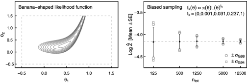
Figure 1: The banana-shaped likelihood function of our first case study [Equation (4) of Section 4] illustrated graphically as a logarithmically-spaced contour plot on the domain of our Uniform prior, $[-0.5,1.5]\times[-0.5,1.5]$ (left-hand panel). Convergence of the biased sampling estimator for the corresponding marginal likelihood under MC³ sampling of the power posterior (at five prespecified temperatures) as a function of the total sample size is shown in the right-hand panel. The marked points and error bars on this figure indicate respectively the recovered mean and standard error (SE) in $\log\hat{Z}$ for 100 trials at each $n_{\mathrm{tot}}$. The dashed, light grey line indicates the “exact” $\log Z$ for this example derived via brute-force quadrature, and the open, light grey symbols indicate the mean “per simulation” estimate of the SE from the asymptotic covariance matrix formulae of Gill, Vardi and Wellner (1988) and Geyer (1994) alternately.

To show the equivalence between this estimator and that of the recursive update scheme defined by Equation (2), we simply observe that the derivative of the denominator in Equation (3) equals the numerator and, thus, by analogy to $\int_{0}^{1}s^{\prime}(x)/s(x)\,dx=\log s(1)-\log s(0)$, we have

$$\log(\hat{Z}_{k}/\hat{Z}_{k-1}) = \log\Biggl{[}\sum_{i=1}^{n}g_{k}(\theta_{i})/p(\theta_{i})\Biggr{]}$$

$${}-\log\Biggl{[}\sum_{i=1}^{n}g_{k-1}(\theta_{i})/p(\theta_{i})\Biggr{]},$$

and, thus,

$$\log\hat{Z}_{k}=\log\Biggl{[}\sum_{i=1}^{n}g_{k}(\theta_{i})/p(\theta_{i})/n\Biggr{]}.$$

In the following two case studies we further explore by numerical example various issues concerning the design of the bridging sequence [with particular reference to the efficiency in $L(y|\theta)$ calls; Section 4], and we highlight the utility of the normalized bridging sequence for prior-sensitivity analysis (Section 5).

4 Case Study: Banana-Shaped LIkelihood Function

For our first case study we consider a (“mock,” that is, data independent) banana-shaped likelihood function, defined in two dimensions ($\theta=\{\theta_{1},\theta_{2}\}$) as

$$L(\theta) = \exp\bigl{(}-\bigl{(}10\times(0.45-\theta_{1})\bigr{)}^{2}/4$$

$$\phantom{\exp\bigl{(}\ \,\,}{}-\bigl{(}20\times\bigl{(}\theta_{2}/2-\theta_{1}^{4}\bigr{)}\bigr{)}^{2}\bigr{)},$$

with a Uniform prior density of $\pi(\theta)=1/4$ on the rectangular domain, $[-0.5,1.5]\times[-0.5,1.5]$. A simple illustration of this likelihood function as a logarithmically-spaced contour plot is presented in the left-hand panel of Figure 1. Brute-force numerical integration via quadrature returns the “exact” solution, $Z=0.01569[6]$ (or $\log Z=-4.154[3]$).

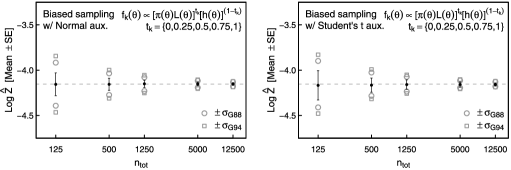
Figure 2: Convergence of the biased sampling estimator for the marginal likelihood of our banana-shaped likelihood function under MC³ sampling (at five prespecified temperatures) on the geometric path between a “data-driven” reference/auxiliary density, $h(\theta)$, and the posterior, shown as a function of the total sample size. The adopted $h(\theta)$ takes a two-dimensional Student’s $t$ form in the left-hand panel and a Normal form in the right-hand, with its controlling parameters ($\mu_{\mathrm{mode}}$ and $\Sigma_{\mathrm{mode}}$) in each case set to the location and curvature of the posterior mode. A marked reduction in standard error (at fixed $n_{\mathrm{tot}}$) with respect to that of the naïve (power posteriors) path, that is, $h(\theta)=\pi(\theta)$, is evident from comparison with Figure 1.

As a benchmark of the method we first apply the biased sampling estimator to draws from a sequence of bridging densities following the standard power posteriors path. Though even a cursory inspection of the likelihood function for this simple case study is sufficient to confirm its unimodality and to motivate a family of suitable proposal densities for straightforward importance sampling of $\pi_{t}(\theta)\propto\pi(\theta)L(\theta)^{t}$, for demonstrative purposes we have chosen to implement an MC³ ((Geyer, 1992)) approach here instead, the latter being ultimately amenable to more complex posteriors than the former. Following standard practice for thermodynamic integration—as per our motivation from Sections 2.4 and 3 above—we adopt a prespecified tempering schedule spaced geometrically as $t=\{0,1/(m-1),2/(m-1),\ldots,1\}^{c}$ with $c=5$ and $m=5$. To illustrate the $1/\sqrt{n}$ convergence of biased sampling, we run this procedure 100 times at each of five total sample sizes ($n_{\mathrm{tot}}=\{125,500,1250,5000,12\mbox{,}500\}$; distributed equally across all five temperatures) thinned at a rate of 0.25 from their parent MC³ chains. The resulting mean and standard error (SE) at each $n_{\mathrm{tot}}$ are marked in the right-hand panel of Figure 1.

Overlaid are (the means of) the corresponding “per simulation” estimates of this standard error computed from the rival asymptotic covariance matrix forms of Gill, Vardi and Wellner (1988)/Kong et al. (2003) and Geyer (1994): the former being originally derived from the empirical process CLT applicable to biased sampling and the latter from maximum likelihood theory using the Hessian of the quasi-likelihood function for reverse logistic regression. As noted in Section 2, Kong et al. (2003) have previously discussed the inadequacy of Geyer’s covariance estimator—though for the present design the difference is negligible. It is worth noting that both estimates are a little conservative at low $n_{\mathrm{tot}}$ but give an excellent agreement with the repeat simulation SE by $n_{\mathrm{tot}}=1250$.

With this power posteriors version of biased sampling as benchmark, we now consider the merits of two alternative schemes for defining, and sampling from, the required sequence of bridging densities, $f_{k}(\theta)$, in Sections 4.1 and 4.2 below.

4.1 Thermodynamic Integration from a Reference/Auxiliary Density

As highlighted by Lefebvre, Steele and Vandal (2010), the error budget of thermodynamic integration over the geometric path depends to first-order upon the $J$-divergence between the reference/auxiliary density, $h(\theta)$, and the target, $\pi(\theta|y)$. Thus, it will generally be more efficient to set a “data-driven” $h(\theta)$—such as may be recovered from the position and local curvature of the posterior mode—than to integrate “naïvely” from the prior, that is, $h(\theta)=\pi(\theta)$. Here we demonstrate the corresponding improvement to the performance of the biased sampling estimator resulting from the choices, $h(\theta)\sim\mathcal{N}_{\mathrm{Trunc.}}(\mu_{\mathrm{mode}},\Sigma_{\mathrm{mode}}^{-1})$ and $h(\theta)\sim\mathcal{T}_{\mathrm{Trunc.}}(\mu_{\mathrm{mode}},\Sigma_{\mathrm{mode}}^{-1})$. Here $\mathcal{N}_{\mathrm{Trunc.}}$ and $\mathcal{T}_{\mathrm{Trunc.}}$ denote the two-dimensional Normal and Student’s $t$ ($\nu=1$) distributions (truncated to our prior support), respectively, while $\mu_{\mathrm{mode}}$ denotes the posterior mode and $\Sigma_{\mathrm{mode}}$ its local curvature (recovered here analytically, but estimable at minimal cost in many Bayesian analysis problems via standard numerical methods). As before, we apply MC³ to explore the tempered posterior and repeat both experiments 100 times at each of our five $n_{\mathrm{tot}}$. In contrast to the power posteriors case, we adopt here a regular temperature grid, $t=\{0,0.25,0.5,0.75,1\}$, to allow for the imposed/intended similarity between $\pi(\theta|y)$ and $h(\theta)$. Our results are presented in Figure 2 and discussed below.

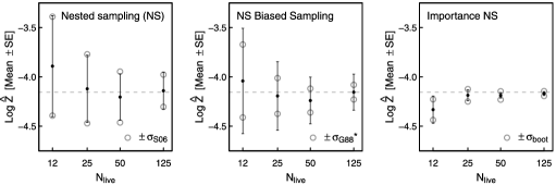
Figure 3: The performance of nested sampling (left-hand panel) as a marginal likelihood estimator for our banana-shaped pseudo-likelihood function, run under the ellipse-based strategy for exploring the sequence of constrained-likelihood densities proposed by Mukherjee, Parkinson and Liddle (2006); compared with that of biased sampling (middle panel) and “importance nested sampling” (right-hand panel) with the same bridging sequence. The first two schemes converge to the true $\log Z$ at a similar rate in $N_{\mathrm{live}}$, while the third is faster since it harnesses the information content of draws otherwise discarded from nested sampling in its constrained-likelihood search.

As expected from both theoretical considerations ((Gelman and Meng, 1998); (Lefebvre, Steele and Vandal, 2010)) and reports of practical experience with other marginal likelihood estimators ((Fan et al., 2012)), use of a “data-driven” auxiliary in this example has indeed reduced markedly the standard error of the biased sampling scheme (at fixed $n_{\mathrm{tot}}$) with respect to that of the naïve (power posteriors) path, that is, $h(\theta)=\pi(\theta)$. In this instance the (thinner-tailed) Normal auxiliary has outperformed the (fatter-tailed) Student’s $t$ (with one d.o.f.); however, although this result is again consistent with theoretical expectations—as a quick computation using the “exact” $\log Z$ confirms $J[\mathcal{N}(\mu_{\mathrm{mode}},\Sigma_{\mathrm{mode}}^{-1}),h(\theta)]\ll J[\mathcal{T}(\mu_{\mathrm{mode}},\Sigma_{\mathrm{mode}}^{-1}),h(\theta)]$—it should be remembered that the optimal choice of auxiliary from within a standard parametric family depends on the likelihood function itself, and so will vary from problem to problem. Moreover, without knowledge of the desired $Z$ it is not possible to optimize $h(\theta)$ a priori; and even a crude estimator of the $J$-divergence run with, for example, the Laplace approximation to the marginal likelihood will nevertheless add numerous extra likelihood evaluations to the computational budget. Although “fatter-tailed” than a typical likelihood function, the Student’s $t$ may well prove a superior choice for some multimodel posterior problems in practice by better facilitating mixing during the MC³ sampling stage.

4.2 Ellipse/Ellipsoid-Based Nested Sampling

Recalling the connections between the DoS derivation of the recursive pathway and the nested sampling algorithm described in Section 2.2, it is of some interest to compare directly the performance of these rival techniques. The present case study with its Uniform prior density is in fact well suited to this purpose since in the field of cosmological model selection, where nested sampling has been most extensively used of late ((Mukherjee, Parkinson and Liddle, 2006); (Feroz and Hobson, 2008)), it is standard practice to adopt separable priors from which a Uniform sample space may be easily constructed under the quantile function transformation, which, for the discussion below, we assume has been done such that $\pi(\theta)$ may be taken as strictly Uniform on $[0,1]^{N}$ (in the transformed coordinate space). Given these conditions, Mukherjee, Parkinson and Liddle (2006) outline a crude-but-effective scheme for exploring the constrained-likelihood shells of nested sampling, in which the new “live” particle for each update must be drawn with density proportional to $\pi(\theta)I(L(\theta)>L(\theta_{i-1}))$.

Under the Mukherjee, Parkinson and Liddle (2006) scheme, to draw the required $\theta_{i}$, one simply identifies the minimum bounding ellipse [or with $D(\theta)>2$, the minimum bounding ellipsoid] for the present set of “live” particles, expands this ellipse by a small factor $\sim$1.5–2 with the aim of enclosing the full support of $I(L(\theta)>L(\theta_{i-1}))$, and then draws randomly from its interior until a valid $\{\theta_{i},L(\theta_{i})\}$ is discovered. Supposing the elliptical sampling window thus defined has been enlarged sufficiently to fully enclose the desired likelihood surface [which it must do to ensure unbiased sampling of $\{\theta_{i},L(\theta_{i})\}$, although we can rarely be sure that it has], it remains unlikely to match its shape exactly, leading to an overhead of $n_{\mathrm{oh}}$ discarded draws, $\{\theta_{i}^{(j)}\dvtx L(\theta_{i}^{(j)})<L(\theta_{i-1}),j=1,\ldots,n_{\mathrm{oh}}\}$. At each $\theta_{i}$ the incurred $n_{\mathrm{oh}}$ may be thought of as a single realization of the negative binomial distribution with $p$ equal to the fraction of the bounded ellipse for which $L(\theta)<L(\theta_{i-1})$, hence, $E(n_{\mathrm{oh}})=1/p-1$. The magnitude of this overhead can in general be expected to scale with the geometric volume of the parameter space, potentially limiting the utility of this otherwise dimensionally-insensitive Monte Carlo-based estimator. However, where applicable, the Mukherjee, Parkinson and Liddle (2006) scheme may nevertheless prove more efficient than the alternative of constrained-MCMC-sampling to find the new $\theta_{i}$ (cf. Friel and Wyse, 2012) in which one must discard at least $\sim$10–20 burn-in moves [each with a necessary $L(\theta)$ call] per step to achieve approximate stationarity.

Applying the ellipse-based approach to nested sampling of the banana-shaped likelihood function of Equation (4) with $N_{\mathrm{live}}=\{12,25,50,125\}$ live particles evolved over $10\times N_{\mathrm{live}}$ steps in each case [and a small extrapolation of the mean $L_{\mathrm{live}}$ times $\exp(-10)$ at the final step; cf. Skilling, 2006], we recover a convergence to the true $\log Z$ as shown in the left-hand panel of Figure 3. Important to note is that with the ellipse scale factor of 1.5 used here the result is an overhead of $n_{\mathrm{oh}}\approx 2.3$ likelihood calls per accepted $\theta_{i}$, such that nested sampling at $N_{\mathrm{live}}=125$ corresponds to $n_{\mathrm{tot}}\approx 2875$ in the previous examples. An overhead of this magnitude should be a concern for “real world” applications of nested sampling in which the likelihood function may be genuinely expensive to evaluate; indeed, for modern cosmological simulations MCMC exploration of the $D(\theta)\lesssim 12$ posterior is effectively a super-computer-only exercise due solely to the cost of solving for $L(y|\theta)$. [At this point the skeptical reader might object that the distinctly nonelliptical $L(\theta)$ considered in this example be considered a particularly unfair case for testing the Mukherjee, Parkinson and Liddle (2006) method, but such banana-shaped likelihoods are in fact quite common in higher-order cosmological models; see, for instance, Davis et al. (2007).] We therefore suggest that one might improve upon the efficiency of ellipse-based nested sampling by co-opting its bridging sequence into the biased sampling framework in some manner.

As Habeck (2012) has pointed out, the nested sampling pathway can be accommodated roughly within the DoS (and hence biased sampling) framework, for example, by treating the accepted $\theta_{i}$ (pooled with the surviving $N_{\mathrm{live}}$ live particles) as drawn from the series of weighted distributions, $w_{j}(\theta)\,dF(\theta)=I(L(\theta)>L_{j})\,dF(\theta)$. However, with each $w_{j}(\theta)$ ($j>1$) now dependent on past draws—and hence the $\{\theta_{i}\}_{j}$ no longer i.i.d.—although we can apply the recursive update scheme of Equation (2) to normalize the bridging sequence and then importance sample reweight to $Z$, the biased sampling CLT no longer holds. To demonstrate this, we apply the above procedure to the draws from our previous nested sampling runs and plot the mean and repeat simulation SE at each $N_{\mathrm{live}}$ in the middle panel of Figure 3. While the efficiency of this estimator is almost identical to that of ordinary nested sampling, the “naïve” application of Gill et al.’s asymptotic covariance matrix does not yield an SE estimate matching that of repeat simulation.

A more interesting alternative is to observe that for the ellipse-based nested sampling method (given uniform priors) the normalization of each $f_{k}(\theta)$ is in fact easily computed from the area/volume of the corresponding ellipse/ellipsoid. That is, we can simply pool our draws—including the $\theta_{i}$ with $L(\{\theta_{i}\}_{j})<L_{j}$ otherwise discarded from nested sampling—and apply the importance sample reweighting procedure of Equation (13) with $\pi_{\mathrm{alt}}(\theta)=\pi(\theta)$ and

$$p(\theta)=\sum_{k=1}^{m}[n_{k}/n_{\mathrm{tot}}]\bigl{[}I\bigl{(}\theta\in\mathit{Ell}[E_{\mathrm{live}(k)}]\bigr{)}/V_{k}\bigr{]}$$

(with $V_{k}$ the volume of the $k$th ellipse and $\mathit{Ell}[E_{\mathrm{live}(k)}]$ its interior). Application of this strategy—which we dub “importance nested sampling” (INS)—to the present example yields $\log Z$ estimates with much smaller repeat simulation SE than either of the previous summations as shown in the right-hand panel of Figure 3. Bootstrap resampling of the drawn $\{\theta_{i},L_{i}\}$ gives a reasonable estimator of this SE, though we note that INS does not appear to be unbiased in $\log Z$, with a slight tendency toward underestimation at small $n_{\mathrm{tot}}$. Further computational experiments are now underway to better quantify the advantages offered by this approach to harnessing the information content of these otherwise discarded draws in the ellipse-based nested sampling paradigm (presented in Feroz et al., 2013).

5 Case Study: Normal Mixture Modeling of the Galaxy Data Set

The well-known galaxy data set, first proposed as a test case for kernel density estimation by Roeder (1990), consists of precise recession velocity measurements (in units of 1000 km s^-1) for 82 galaxies in the Corona Borealis region of the Northern sky reported by Postman, Huchra and Geller (1986). The purpose of the original astronomical study was to search—in light of a then recently discovered void in the neighboring Boötes field ((Kirshner et al., 1981))—for further large-scale inhomogeneities in the distribution of galaxies. Given the well-defined selection function of their survey, Postman, Huchra and Geller (1986) were easily able to compute as a benchmark the recession velocity density function expected under the null hypothesis of a uniform distribution of galaxies throughout space, and by visual comparison of this density against a histogram of their observed velocities the astronomers were able to establish strong evidence against the null, thereby boosting support for the (now canonical) hierarchical clustering model of cosmological mass assembly ((Gunn, 1972)). However, under the latter hypothesis, as Roeder (1990) insightfully observed, one can then ask the more challenging statistical question of “how many distinct clustering components are in fact present in the recession velocity data set?”

Many authors have since attempted to answer this question (posed for simplicity as a univariate Normal mixture modeling problem) as a means to demonstrate the utility of their preferred marginal likelihood estimation or model space exploration strategy. Notable such contributions to this end include the following: the infinite mixture model (Dirichlet process prior) analyses of Escobar and West (1995) and Phillips and Smith (1996); Chib’s exposition of marginal likelihood estimation from Gibbs sampling output ((Chib, 1995)); the reversible jump MCMC approach of Richardson and Green (1997); and the label switching studies of Stephens (2000) and Jasra, Holmes and Stephens (2005). The earliest of these efforts are well summarized by Aitkin (2001), who highlights a marked dependence of the inferred number of mixture components on the chosen priors. For this reason, as much as its historical significance, the galaxy data set provides a most interesting case study with which to illustrate the potential of prior-sensitivity analysis under the recursive pathway.

The outline of our presentation is as follows. In Section 5.1 we set forth the finite and infinite mixture models to be examined here and in Section 5.2 we describe the MCMC strategies we use to explore their complete and partial data posteriors. In Section 5.3 we discuss various astronomical motivations for our default hyperprior choices and, finally, in Section 5.4 we present the results of a biased sampling run on this problem with importance sample reweighting-based transformations between alternative priors.

5.1 Normal Mixture Model

5.1.1 Finite mixture model

Following Diebolt and Robert (1994) and Lee et al. (2008), we write the $k$-component Normal mixture model with component weights, $\phi$, in the latent allocation variable form for data vector, $y$, and (unobserved) allocation vector, $z$, such that

$$\pi(z_{i}=j)=\phi_{j}\quad\mbox{and}\quad\pi(y_{i}|z_{i}=j)=f_{\mathcal{N}}(y_{i}|\theta_{j}).$$

Here $f_{\mathcal{N}}(\cdot|\theta_{j})$ represents the one-dimensional Normal density, which we will reference in mean–precision syntax as $\mathcal{N}(\mu_{j},\tau_{j}^{-1})$, that is, $\theta_{j}=\{\mu_{j},\tau_{j}\}$.

Given priors for the number of components in the mixture, the distribution of weights at a given $k$ and the vector of mean precisions—that is, $\pi(k)$, $\pi(\phi|k)$ and $\pi(\theta|\phi,k)$, respectively—the posterior for the number of mixture components in the finite mixture case may be recovered by integration over $\{\phi,\theta\}$ at each $k$,

$$\pi(k|y) = \pi(k)/Z$$

$${}\times\int_{\Omega}\pi(\phi|k)\pi(\theta|\phi,k)L(y|\theta,\phi,k)\,d\phi\,d\theta$$

$$= \pi(k)Z^{(k)}/Z.$$

Here the likelihood, $L(y|\theta,\phi,k)$, is given by a summation over the $n_{\mathrm{tot}}$ unobserved, $z_{i}$, as

$$L(y|\theta,\phi,k)=\prod_{i=1}^{n_{\mathrm{tot}}}\sum_{j=1}^{k}\phi_{j}f_{\mathcal{N}}(y_{i}|\theta_{j}).$$ (18)

That is, for a $\pi(k)$ assigning mass to only a small set of elements, one approach to recovering $\pi(k|y)$ is simply to estimate the “per component” marginal likelihood, $\hat{Z}^{(k)}$, at each of these $k$ and then reweight by $\pi(k)$. The full marginal likelihood of the model can then of course be estimated from the sum, $\hat{Z}=\sum_{k}\hat{Z}^{(k)}$. While this is indeed the strategy adopted here for exposition purposes, it is worth noting that such direct marginal likelihood estimation to recover $\pi(k|y)$ for this model can in fact be entirely avoided via either the reversible jump MCMC algorithm ((Richardson and Green, 1997)) or Gibbs sampling over the infinite mixture version described below.

5.1.2 Infinite mixture model

Rather than specify a maximum number of mixture components a priori, Escobar and West (1995) and Phillips and Smith (1996) (among others) have advocated an infinite-dimensional solution based on the Dirichet process prior. In particular, one may suppose the data to have been drawn from an infinite mixture of Normals with means, variances and weights drawn as the realization, $Q$, of a Dirichlet process (DP), $\operatorname{DP}(M,G_{0})$, on $\mathbb{R}\times\mathbb{R}_{+}$, the characterization of the DP being via a concentration index, $M$, and reference density, $G_{0}$, and with all $Q$ being both normalized and strictly atomic. For small $M$ ($\lesssim 10$) the tendency is for these $Q$ to be dominated by only a few (mixture) components, while for large $M$ the number of significant components inevitably increases, with the typical $Q$ thereby becoming closer (in the metric of weak convergence) to $G_{0}$. The likelihood of i.i.d. $y$ for a given $Q$ requires (in theory) an infinite sum over the contribution from each of its components,

$$L(y|Q)=\prod_{i=1}^{n_{\mathrm{tot}}}\sum_{j=1}^{\infty}\phi_{j}f_{\mathcal{N}}(y_{i}|\theta_{j}),$$

where each $\phi_{j}$ represents the limiting fraction of points in the realization assigned to a particular $\theta_{j}$. (In practice, however, this summation can generally be truncated with negligible loss of accuracy after accounting for the contributions of only the most dominant components.) Computation of the marginal likelihood for the above model is thus nominally by integration over the infinite-dimensional space of $Q$. In particular, if we suppose a hyperprior density for the hyperparameters, $\psi$, of the DP (i.e., for $M$ and the controlling parameters of $G_{0}$), we have $Z=\int_{\Omega(\psi)}\int_{\Omega(Q)}L(y|Q)\{dP_{Q|\psi}(Q)\}\pi(\psi)\,d\psi$.

As per the finite mixture case, we can simplify our posterior exploration and relevant computations by introducing latent variables, $z$ and $\theta$, for allocation of the $y$ and the corresponding mean-precision vectors of the parent components in $Q$. In this version the likelihood takes the form

$$L\bigl{(}y|\{z,\theta\}\bigr{)}=\prod_{i=1}^{n_{\mathrm{tot}}}f_{\mathcal{N}}(y_{i}|\theta_{z_{i}}),$$

and the marginal likelihood becomes

$$Z = \int_{\Omega(\psi)}\int_{\Omega(Q)}\int_{\Omega(\{z,\theta\})}L\bigl{(}y|\{z,\theta\}\bigr{)}$$

$$\phantom{\int_{\Omega(\psi)}\int_{\Omega(Q)}\int_{\Omega(\{z,\theta\})}}{}\cdot\bigl{\{}dP_{\{z,\theta\}|Q}\bigl{(}\{z,\theta\}\bigr{)}\bigr{\}}$$

$$\phantom{\int_{\Omega(\psi)}\int_{\Omega(Q)}\int_{\Omega(\{z,\theta\})}}{}\cdot\bigl{\{}dP_{Q|\psi}(Q)\bigr{\}}\pi(\psi)\,d\psi.$$

Importantly, existing Gibbs sampling methods for the DP allow for collapsed sampling from the posterior for $\{z,\theta,\psi\}$ and Equation (5.1.2) can be reduced to $\int_{\Omega(\{z,\theta,\psi\})}L(y|\{z,\theta\})\{dP_{\{z,\theta,\psi\}}(\{z,\theta,\psi\})\}$. In one further twist, however, we note that since the reduced expression is degenerate across component labelings, it is in fact more computationally efficient to estimate $Z$ from

$$\int_{\Omega(\{z,\theta,\psi\})}\int_{\Omega(\hat{Q})}L(y|\hat{Q})$$

$$\phantom{\int_{\Omega(\{z,\theta,\psi\})}\int_{\Omega(\hat{Q})}}{}\cdot\{dP_{\hat{Q}|\{z,\theta,\psi\}}\}$$ (20)

$$\phantom{\int_{\Omega(\{z,\theta,\psi\})}\int_{\Omega(\hat{Q})}}{}\cdot\bigl{\{}dP_{\{z,\theta,\psi\}}\bigl{(}\{z,\theta,\psi\}\bigr{)}\bigr{\}},$$

where $P_{\hat{Q}|\{z,\theta,\psi\}}$ takes a particularly simple analytic form by the nature of the DP (cf. Escobar and West, 1995).

Finally, it is important to note that since each realization of the DP has always an infinite number of components with probability one (though usually only a few with significant mass), the usual interpretation for the posterior, $\pi(k|y)$, in this context is the posterior distribution of the number of unique label assignments among the observed data set (i.e., the dimension of $\theta$ in $\{z,\theta\}$). However, although pragmatically useful for such modeling problems as that exhibited by the galaxy data set, as Miller and Harrison (2013) note, this estimate is not consistent.

5.2 MC Exploration of the Mixture Model Posterior

5.2.1 Finite mixture model

Exploration of the posterior for $\{\theta,\phi\}$ at fixed $k$ in this finite mixture model can be accomplished rather efficiently (modulo the well-known problem of mixing between modes; cf. Neal, 1999) via Gibbs sampling given conjugate prior choices, as explained in detail by Richardson and Green (1997). To this end, we suppose

$$\mu_{j} \sim \mathcal{N}\bigl{(}\kappa,\xi^{-1}\bigr{)},\quad\tau_{j}\sim\Gamma(\alpha,\beta),\quad\mbox{and}$$

$$\beta \sim \Gamma(\beta_{1},\beta_{2}),$$

where $\Gamma(a,b)$ represents the Gamma distribution with rate $a$ and shape $b$. To simulate from the resulting posterior, we use the purpose-built code provided by BMMmodel and JAGSrun in the BayesMix package ((Grün and Leisch, 2010)) for R. No modifications to this code are necessary for sampling the partial data posterior, and both the partial and full data likelihoods given partial likelihood draws (at fixed $k$) may be recovered with Equation (18). The range of $k$ for which we compute marginal likelihoods is here limited by the range of a truncated Poisson prior on $k$.

5.2.2 Infinite mixture model

As noted earlier, exploration of the infinite mixture model posterior can also be facilitated through Gibbs sampling with the appropriate choice of priors ((Escobar and West, 1995)); and although contemporary codes typically use the (more efficient) alternative algorithm of Neal (2000), the prior forms dictated by the conjugacy necessary for Gibbs sampling remain the default. Hence, to this end, we suppose a fixed concentration index of $M=1$ and a Normal-Gamma reference density,

$$G_{0}\dvtx\tau_{j}\sim\Gamma(s/2,S/2),\quad\mu_{j}|\tau_{j}\sim\mathcal{N}(m,\tau_{j}h),$$

assigning hyperpriors of $h\sim\Gamma(h_{1}/2,h_{2}/2)$ and $1/S\sim\Gamma(\nu_{1}/2,\nu_{2}/2)$. Here we use the DPdensity function in the DPpackage ((Jara et al., 2011)) for R to explore this posterior. While no modifications to this code are required for sampling the partial likelihood posteriors, the computation of full data likelihoods given the partial likelihood posterior requires that we sample a series of dummy components from the current posterior until some appropriate truncation point, $k^{\prime}\dvtx\sum_{j=1}^{k^{\prime}}\phi_{j}\approx 1$, before applying (the $k^{\prime}$-truncated version of) Equation (5.1.2).

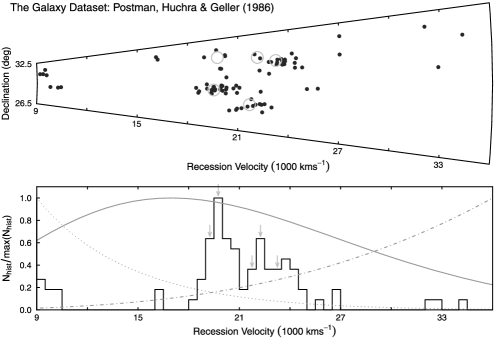
Figure 4: Visualization of the galaxy data set, including its Abell clusters and selection function. The clustering of galaxies in recession velocity–declination space is illustrated by way of the “cone diagram” shown in the top panel and its projection to a recession velocity histogram shown in the bottom panel. The positions of five Abell clusters targeted by the original survey are also highlighted here (open circles and arrows in light grey), along with the survey’s magnitude-dependent, volume-dependent and net selection functions (shown as the dotted, dash-dotted and solid curves, respectively, in the bottom panel).

5.3 Astronomical Motivations for our Priors

5.3.1 Finite mixture model

As noted earlier, by considering the well-defined selection function of their observational campaign, the authors of the original astronomical study were able to construct the expected probability density function of recession velocities for their survey under the null hypothesis of a uniform distribution of galaxies throughout space. In particular, Postman, Huchra and Geller (1986) recognized that the strict apparent magnitude limit of their spectroscopic targeting strategy ($m_{r}<15.7$ mag) would act as a luminosity (or absolute magnitude) limit evolving with recession velocity (distance) according to

$$M_{r,\mathrm{lim}}(v)\approx m_{r}-5\log_{10}(v)-30,$$

where we have assumed units of 1000 km s^-1 for $v$ and a “Hubble constant” of $H_{0}=100$ km s^-1 Mpc^-1. To estimate the form of the resulting selection function, $S_{\mathrm{mag}}(v)$, Postman, Huchra and Geller (1986) considered how the relative number of galaxies per unit volume brighter than this limit would vary with distance given the absolute magnitude distribution function, $F_{\mathrm{mag}}(\cdot)$, for galaxies in the local Universe, that is, $S_{\mathrm{mag}}(v)\propto 1-F_{\mathrm{mag}}(M_{r,\mathrm{lim}}(v))$. To approximate the latter, the astronomers simply integrated over a previous estimate of the local luminosity density parameterized as a Schechter function ((Schechter, 1976)) with characteristic magnitude, $M_{r}^{\ast}\approx-19.40-1.5$ mag, and faint-end slope, $\alpha_{r}^{\ast}\approx-1.3$, such that

$$f(M)\propto\bigl{[}10^{2/5(M_{r}^{\ast}-M)}\bigr{]}^{\alpha_{r}^{\ast}+1}\exp\bigl{[}-10^{2/5(M_{r}^{\ast}-M)}\bigr{]}$$

and

$$S_{\mathrm{mag}}(v)\propto\int_{-\infty}^{M_{r,\mathrm{lim}}(v)}f(M)\,dM.$$

An interesting feature of magnitude-limited astronomical surveys is that, although with increasing recession velocity this $S_{\mathrm{mag}}(v)$ selection function restricts their sampling to the decreasing fraction of galaxies above $M_{r,\mathrm{lim}}(v)$, the volume of the Universe probed by (the projection into three-dimensional space of) their two-dimensional angular viewing window is, in contrast, rapidly increasing. Hence, there exists an important additional selection effect, $S_{\mathrm{vol}}(v)$, operating in competition with, and initially dominating, that on magnitude, and scaling with (roughly) the third power of recession velocity such that

$$S_{\mathrm{vol}}(v)\propto v^{3}.$$

The product of these two effects therefore returns the net selection function of the galaxy data set, which we illustrate (along with each effect in isolation) in Figure 4 (see also Figure 4b from Postman, Huchra and Geller, 1986); the point being that there do exist informative astronomical considerations for choosing at least some of the hyperparameters of our priors in this mixture modeling case study, though past analyses have tended to ignore this context (contributing somewhat to the apparent “failure” of Bayesian mixture modeling for this data set; Aitkin, 2001). In particular, the shape of the selection function in velocity space suggests the form for our prior on the component means: a choice of $\{\kappa=17,\xi=0.008\}$ gives a reasonable match to the shape of $S_{\mathrm{mag}}(v)S_{\mathrm{vol}}(v)$. Perhaps surprisingly, as we will demonstrate later, the choice of prior on the component means has a substantial influence on the resulting $\pi(k|y)$; changing only these of our hyperparameters to “data-driven” values chosen as $\{\kappa=\bar{y}\ (20.8),\xi=1/\operatorname{var}\{y\}\ (0.048)\}$ results in a drastic shift of the posterior.

Likewise, we can inform our prior choice for the number of components in the mixture with regard to the original survey design, which featured five separate observational windows placed so as to cover five previously identified galaxy clusters from the Abell catalog. (The positions of these clusters in bivariate recession velocity–declination space, and its projection to univariate velocity space, are also marked on Figure 4 for reference.) Hence, we select a mode of $\lambda=5$ for our truncated Poisson prior for $\pi(k)$. With the $k=1$ and $k=2$ mixture models already well excluded by previous analyses, and $k>10$ a pragmatic upper bound for exploration given $\lambda=5$, we therefore truncate our prior to the range $3\leq k\leq 10$. This contrasts somewhat with the Uniform priors on $k\leq 10$ and $k\leq 30$ assumed by Roeder and Wasserman (1997) and Richardson and Green (1997), respectively—though reweighting for alternative $\pi(k)$ (on this support) is trivial in any case.

Only the precisions of the Normal mixture components are not well constrained from astronomical considerations—although we can at least be confident that any large-scale clustering should occur above the scale of individual galaxy clusters ($\sim$1 Mpc or $\Delta v\approx 0.1$) and (unless the uniform space-filling hypothesis were correct) well below the width of our selection function. Thus, we simply adopt a fixed shape hyperparameter of $\alpha=2$ for our Gamma prior on the $\tau_{j}$ and allow the rate hyperparameter to vary according to its Gamma hyperprior form $\beta_{1}=1$ and $\beta_{2}=0.05$. Our choice here is thus comparable to that of Richardson and Green (1997) who suppose $\pi(\beta)\sim\Gamma(0.2,0.016)$—not $\Gamma(0.2,0.573)$ as misquoted by Aitkin (2001)—though we evidently place far less prior weight on exceedingly large precisions (small variances).

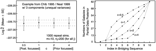
Figure 5: Relationship between the standard error (SE) of $\log Z$ estimation and the choice of a partial data posterior bridging sequence for biased sampling of the 3-component (unequal variance) mixture model under the Chib (1995) priors. The data points in the left-hand panel represent the mean $\log\hat{Z}$ and the error bars its (single run) SE, computed from 1000 repeat simulations with 200 draws from each of 10 steps in the bridging sequence. The dashed grey lines indicate the benchmark estimate ($\pm\,$SE) from Neal (1999), and the $c$ values of the horizontal axis refer to the design of the partial data posterior bridging sequence as $r_{j}=n_{\mathrm{tot}}\times\{0,1/9,2/9,\ldots,1\}^{c}$. These sequences are also illustrated graphically for clarity in the right-hand panel.

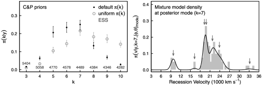
Figure 6: Posterior probabilities for the number of Normal mixture components in the galaxy data set, $\pi(k|y)$, under our astronomically motivated priors (left-hand panel). The solid, dark grey symbols here denote the true posterior, while the open, light grey symbols indicate for reference the raw, “per component” marginal likelihood-based result, that is, before application of our truncated Poisson $\pi(k)$. In each case the relevant uncertainties [recovered from estimates of the asymptotic covariance matrix for each $\log\hat{Z}^{(k)}$] are illustrated as 95% credible interval error bars. The effective sample size (ESS) provided by the pseudo-mixture of 10 partial data posteriors sampled for 4000 draws each is noted in grey for each $k$. The inferred probability density (in velocity space) at the maximum a posteriori parameterization of our Normal mixture model ($k=7$) is then illustrated for reference against a scaled histogram of the galaxy data set in the right-hand panel.

5.3.2 Infinite mixture model

The same considerations can also help shape our hyperparameter choices for the priors on our infinite mixture model. In particular, we take $\{m=17,s=4,h_{1}=2,h_{2}=8,\nu_{1}=1,\allowbreak\nu_{2}=1\}$ for the hyperparameters shaping the Normal-Gamma reference density, $G_{0}$, with the aim of matching as closely as possible to the priors of our finite-dimensional model. With the scale parameter of our prior on the component precisions taking an inverse-Gamma hyperprior form in the infinite case and a Gamma form in the finite case, it was not possible to exactly match these distributions: our choice of $\{\nu_{1}=1,\nu_{2}=1\}$ is intended to at least give comparable 5% and 95% quantiles. Finally, we adopt a fixed value for the concentration parameter of $M=1$; this choice coincidentally gives a similar effective prior for the number of unique components among the 82 observed galaxies to that of the $\pi(k)$ adopted for our finite mixture model (see Escobar and West, 1995, for instance).

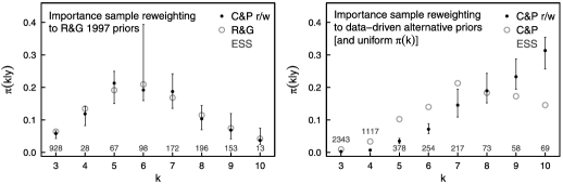
Figure 7: Importance sample reweighting of our draws from the pseudo-mixture of partial data posteriors used to estimate $\pi(k|y)$ under the Richardson and Green (1997) priors (left-hand panel). The solid, dark grey symbols here denote the reweighted posterior estimate, while the open, light grey symbols indicate for reference the Richardson and Green (1997) benchmark. The results of the equivalent procedure to approximate the effect of using alternative “data-driven” priors are shown in the right-hand panel; here the solid, dark grey symbols again represent the reweighted estimate, with the open, light grey symbols illustrating the reference point provided by our default priors. In both instances we treat $\pi(k)$ as uniform to emphasize the difference to the “per component” marginal likelihoods made by this modest change of prior. In each panel the relevant uncertainties [recovered via bootstrap resampling from our pseudo-mixture plus estimates of the asymptotic covariance matrix for each $\log\hat{Z}^{(k)}$] are illustrated as 95% credible interval error bars. The effective sample size (ESS) provided by the pseudo-mixture of 10 partial data posteriors sampled for 4000 draws each is noted in grey for each $k$.

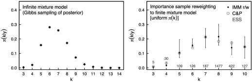
Figure 8: Posterior for the number of unique label assignments among the galaxy data set recovered from Gibbs sampling of our (Dirichlet process-based) infinite mixture model (left-hand panel). The results of importance sample reweighting of these draws, combined as a pseudo-mixture with those simulated under our bridging sequence of partial data posteriors, are shown via the solid, dark grey symbols in the right-hand panel. The target of this reweighting procedure is the “per component” [i.e., uniform $\pi(k)$] posterior for the number of mixture model components in our benchmark finite mixture model (shown as the open, light grey symbols). The relevant uncertainties [recovered via bootstrap resampling from our pseudo-mixture plus estimates of the asymptotic covariance matrix for each $\log\hat{Z}^{(k)}$] are illustrated as 95% credible interval error bars. The effective sample size (ESS) provided by the pseudo-mixture of 10 partial data posteriors sampled for 4000 draws each is noted in grey for each $k$.

5.4 Numerical Results

5.4.1 Chib example

As an initial verification of our code, we first run the Gibbs sampling procedure outlined above (Section 5.2.1) to explore the partial data posteriors of a three-component (unequal variance) mixture model using the priors from Chib (1995), with the biased sampling algorithm then applied for marginal likelihood estimation. Neal (1999) has made public the results of a $10^{8}$ draw AME calculation providing a precise benchmark for the marginal likelihood under these priors of $-226.791\ (\pm\,0.089)$ (SE), though it should be noted that the galaxy data set used for this purpose is that with Chib’s transcription error in the 78th observation (which we insert explicitly into the public R version for the present application only). Given just 200 saved draws from Gibbs sampling (at a thinning rate of 0.9) of the partial data posterior at each of 10 steps spaced as $r_{j}=\lfloor n_{\mathrm{tot}}\times\{0,1/9,2/9,\ldots,1,\}^{c=2}\rfloor$ (with $r_{2}$ reset to 3 to facilitate sampling), we can confirm the recovery of this benchmark as $-226.79\ (\pm\,0.15)$ (SE). Estimation of the (single run) standard error (SE) was for this purpose conducted via 1000 repeat simulations. Further repeats of this procedure with both more posterior focused ($c=0.5$, 1) and more prior focused ($c=4$) partial data schedules confirm the optimality of the $c=2$ choice anticipated from Fisher information principles (Section 2.4). The results of this experiment are illustrated in Figure 5.

5.4.2 Finite mixture model

To estimate “per component” marginal likelihoods for each $k$ ($3\leq k\leq 10$) in our finite mixture model, we run the same procedure of partial data posterior exploration followed by biased sampling with $4000$ draws from each of ten steps on the $c=2$ bridging sequence. The results of this computation are illustrated in Figure 6; the uncertainties indicated are gauged from the asymptotic covariance matrix of the biased sampling estimator (as per Gill, Vardi and Wellner, 1988). We recover a posterior mode of $k=7$ components, the recession velocity density belonging to which at the corresponding mode in $\{\phi,\theta\}$ is also illustrated in Figure 6 for reference. To the eye, it appears that $k=7$ may be a slight overestimate since the third and fourth components (in order of increasing recession velocity) are more or less on top of each other, suggesting that one is being used to account for a slight non-Normality in the shape of this peak.

To demonstrate the potential for efficient prior-sensitivity analysis via importance sample reweighting of the pseudo-mixture density of partial data posteriors normalized by biased sampling (Section 2.3), we begin by recovering the Richardson and Green (1997) result from the above simulation output. The results of this reweighting procedure are shown in Figure 7. Since the Richardson and Green (1997) priors are significantly different to those chosen here from astronomical considerations (as discussed in Section 5.3), the effective sample sizes provided by our pseudo-mixture of $4000\times 10$ draws range from just 13 to 928, yet the resulting approximation to the former benchmark is actually rather good. Moreover, the corresponding 95% credible intervals [recovered via bootstrap resampling from our pseudo-mixture plus estimates of the asymptotic covariance matrix for each $\log\hat{Z}^{(k)}$] indeed enclose all eight $\pi(k|y)$ reference points.

As a second demonstration we also show in Figure 7 the results of reweighting for alternative “data-driven” choices for the hyperparameters of our prior on the component means: $\{\kappa=\bar{y}\ (20.8),\xi=1/\operatorname{var}\{y\}\allowbreak(0.048)\}$. To emphasize the large difference this small change in $\pi(\theta)$ makes to the “per component” log $Z^{(k)}$ values, the comparison presented is between our default and “data-driven” priors with $\pi(k)$ removed (i.e., treated as uniform). This investigation clearly confirms the remarkable prior sensitivity of $\pi(k|y)$ in the galaxy data set example. Interestingly, the preference under our “data-driven” priors is for an even greater number of mixture components ($k>7$), despite the $k=7$ solution already seeming (visually) to be an overfitting of the available data.

5.4.3 Infinite mixture model

In Figure 8 we present the results of Gibbs sampling the posterior of our infinite mixture model. In particular, we show in the left-hand panel of this figure the posterior for the number of unique label assignments among the galaxy data set, which, as we have noted earlier, is typically used as a proxy for the number of mixture components present (although under the Dirichet process prior this is formally always infinite). In the right-hand panel we demonstrate again the power of importance sample reweighting for prior-sensitivity analysis, though for this particular case the stochastic process prior used requires that we apply the appropriate Radon–Nikodym derivative version given by Equation (2.3).

The Radon–Nikodym derivative, $\frac{dP_{\{z,\theta,\psi\},\mathrm{alt}}}{dP_{\{z,\theta,\psi\}}}(\{z,\theta,\allowbreak\psi\})$, of the measure on $\{z,\theta,\psi\}$ assigned by a $k$-component finite mixture model with respect to that assigned by the Dirichlet process prior of our infinite mixture model may be computed as follows. First, we observe that the Radon–Nikodym derivative between two Dirichlet process priors on the (equivalent) space of $\{\{\theta_{1},\ldots,\theta_{n_{\mathrm{tot}}}\},\psi\}$ (with the $\theta_{i}$ possibly nonunique) has been previously derived by Doss (2012), thereby providing a direct formula for computing $\frac{dP_{\{z,\theta,\psi\},\mathrm{int}}}{dP_{\{z,\theta,\psi\}}}(\{z,\theta,\psi\})$, where $P_{\{z,\theta,\psi\},\mathrm{int}}$ represents a Dirichlet process prior with hyperpriors on the $\psi$ of its reference density chosen to be identical to those on the $\{\mu_{j},\tau_{j}\}$ and $\beta$ of our finite mixture model. That is, we choose $P_{\{z,\theta,\psi\},\mathrm{int}}$ such that its projection to $P_{\{z,\theta,\psi\},\mathrm{int}}$ for $z$ with $k$ unique elements is equivalent (a.e.) to that of $P_{\{z,\theta\},\mathrm{alt}}$ with our hyperparameter on $\beta$ integrated out, allowing $P_{\{z,\theta,\psi\},\mathrm{alt}}$ to be defined identical to $f(z)P_{\{z,\theta,\psi\},\mathrm{int}}$. The necessary $f(z)$ to ensure that $\frac{dP_{\{z,\theta,\psi\},\mathrm{alt}}}{dP_{\{z,\theta,\psi\},\mathrm{int}}}\frac{dP_{\{z,\theta,\psi\},\mathrm{int}}}{dP_{\{z,\theta,\psi\}}}=\frac{dP_{\{z,\theta,\psi\},\mathrm{alt}}}{dP_{\{z,\theta,\psi\}}}$ is then simply the ratio of the labeling probabilities under our finite mixture model and the intermediate version of our infinite mixture model [with $f(z)\neq 0$ only where the number of unique elements in $z$ equals $k$].

A formula for the desired $f(z)$ can be derived by combining standard properties of the Dirichlet-Multinomial distribution (our finite-dimensional model prior on $z$) with results from the work of Antoniak (1974) on the marginals of the Dirichlet process. In each case the probability of a given labeling sequence depends not on its ordering, but rather on its vector of per-label counts. Using Antoniak’s system of writing $C(m_{1},m_{2},\ldots,m_{n_{\mathrm{tot}}})$ as the set of labelings with $m_{1}$ unique elements, $m_{2}$ pairs, etc., we have wherever $\sum_{i=1}^{n_{\mathrm{tot}}}m_{i}\leq k$,

$$f(z\in C) = \Biggl{(}\frac{n_{\mathrm{tot}}!}{\prod_{i=1}^{n_{\mathrm{tot}}}(i!)^{m_{i}}}\frac{\Gamma(k\alpha)}{\Gamma(n_{\mathrm{tot}}+k\alpha)}$$

$$\phantom{\qquad\quad}{}\cdot\prod_{i=1}^{n_{\mathrm{tot}}}\biggl{(}\frac{\Gamma(i+\alpha)}{\Gamma(\alpha)}\biggr{)}^{m_{i}}\Biggr{)}$$

$${}\Big{/}\biggl{(}\frac{(k-\sum_{i=1}^{n_{\mathrm{tot}}}m_{i})!(\prod m_{i})!}{k!}$$

$$\hskip 14.22636pt{}\cdot\frac{n_{\mathrm{tot}}!}{\prod_{i=1}^{n_{\mathrm{tot}}}i^{m_{i}}(m_{i}!)}\frac{M^{\sum_{i=1}^{n_{\mathrm{tot}}}m_{i}}}{M^{[n_{\mathrm{tot}}]}}\biggr{)},$$

where $x^{[j]}$ denotes the rising factorial function as per Proposition 3 of Antoniak (1974). For our case of $\alpha=1$ and $M=1$ this reduces to

$$f(z\in C) = \biggl{(}\frac{n_{\mathrm{tot}}!(k-1)!}{(n_{\mathrm{tot}}+k-1)!}\biggr{)}$$

$${}\Big{/}\biggl{(}\frac{(k-\sum_{i=1}^{n_{\mathrm{tot}}}m_{i})!(\prod m_{i})!}{k!\prod_{i=1}^{n_{\mathrm{tot}}}i^{m_{i}}(m_{i}!)}\biggr{)}.$$

6 Conclusions

In this paper we have presented an extensive review of the recursive pathway to marginal likelihood estimation as characterized by biased sampling, reverse logistic regression and the density of states; in particular, we have highlighted the diversity of bridging sequences amenable to recursive normalization and the utility of the resulting pseudo-mixtures for prior-sensitivity analysis (in the Bayesian context). Our key theoretical contributions have included the introduction of a novel heuristic (“thermodynamic integration via importance sampling”) for guiding design of the bridging sequence and an elucidation of various connections between these recursive estimators and the nested sampling technique. Our two numerical case studies illustrate in depth the practical implementation of these ideas using both “ordinary” and stochastic process priors.

References

- Aitkin (2001) {barticle}[auto:STB—2014/02/12—12:18:25] \bauthor\bsnmAitkin, \bfnmM.\binitsM. (\byear2001). \btitleLikelihood and Bayesian analysis of mixtures. \bjournalStatist. Model. \bvolume1 \bpages287–304. \bptokimsref\endbibitem
- Antoniak (1974) {barticle}[mr] \bauthor\bsnmAntoniak, \bfnmCharles E.\binitsC. E. (\byear1974). \btitleMixtures of Dirichlet processes with applications to Bayesian nonparametric problems. \bjournalAnn. Statist. \bvolume2 \bpages1152–1174. \bidissn=0090-5364, mr=0365969 \bptokimsref\endbibitem
- Arima and Tardella (2012) {barticle}[mr] \bauthor\bsnmArima, \bfnmSerena\binitsS. and \bauthor\bsnmTardella, \bfnmLuca\binitsL. (\byear2012). \btitleImproved harmonic mean estimator for phylogenetic model evidence. \bjournalJ. Comput. Biol. \bvolume19 \bpages418–438. \biddoi=10.1089/cmb.2010.0139, issn=1066-5277, mr=2913981 \bptokimsref\endbibitem
- Baele et al. (2012) {barticle}[pbm] \bauthor\bsnmBaele, \bfnmGuy\binitsG., \bauthor\bsnmLemey, \bfnmPhilippe\binitsP., \bauthor\bsnmBedford, \bfnmTrevor\binitsT., \bauthor\bsnmRambaut, \bfnmAndrew\binitsA., \bauthor\bsnmSuchard, \bfnmMarc A.\binitsM. A. and \bauthor\bsnmAlekseyenko, \bfnmAlexander V.\binitsA. V. (\byear2012). \btitleImproving the accuracy of demographic and molecular clock model comparison while accommodating phylogenetic uncertainty. \bjournalMol. Biol. Evol. \bvolume29 \bpages2157–2167. \biddoi=10.1093/molbev/mss084, issn=1537-1719, pii=mss084, pmcid=3424409, pmid=22403239 \bptokimsref\endbibitem
- Bailer-Jones (2012) {barticle}[auto:STB—2014/02/12—12:18:25] \bauthor\bsnmBailer-Jones, \bfnmC. A. L.\binitsC. A. L. (\byear2012). \btitleA Bayesian method for the analysis of deterministic and stochastic time series. \bjournalAstron. Astrophys. \bvolume546 \bpagesA89. \bptokimsref\endbibitem
- Billingsley (1968) {bbook}[mr] \bauthor\bsnmBillingsley, \bfnmPatrick\binitsP. (\byear1968). \btitleConvergence of Probability Measures. \bpublisherWiley, \blocationNew York. \bidmr=0233396 \bptokimsref\endbibitem
- Brewer and Stello (2009) {barticle}[auto:STB—2014/02/12—12:18:25] \bauthor\bsnmBrewer, \bfnmB. J.\binitsB. J. and \bauthor\bsnmStello, \bfnmD.\binitsD. (\byear2009). \btitleGaussian process modelling of asteroseismic data. \bjournalMon. Not. R. Astron. Soc. \bvolume395 \bpages2226–2233. \bptokimsref\endbibitem
- Caimo and Friel (2013) {barticle}[auto:STB—2014/02/12—12:18:25] \bauthor\bsnmCaimo, \bfnmA.\binitsA. and \bauthor\bsnmFriel, \bfnmN.\binitsN. (\byear2013). \btitleBayesian model selection for exponential random graph models. \bjournalSocial Networks \bvolume35 \bpages11–24. \bptokimsref\endbibitem
- Calderhead and Girolami (2009) {barticle}[mr] \bauthor\bsnmCalderhead, \bfnmBen\binitsB. and \bauthor\bsnmGirolami, \bfnmMark\binitsM. (\byear2009). \btitleEstimating Bayes factors via thermodynamic integration and population MCMC. \bjournalComput. Statist. Data Anal. \bvolume53 \bpages4028–4045. \biddoi=10.1016/j.csda.2009.07.025, issn=0167-9473, mr=2744303 \bptokimsref\endbibitem
- Cameron and Pettitt (2013) {bmisc}[auto:STB—2014/02/12—12:18:25] \bauthor\bsnmCameron, \bfnmE.\binitsE. and \bauthor\bsnmPettitt, \bfnmA. N.\binitsA. N. (\byear2013). \bhowpublishedOn the evidence for cosmic variation of the fine structure constant (II): A semi-parametric Bayesian model selection analysis of the quasar dataset. Preprint. Available at \arxivurlarXiv:1309.2737. \bptokimsref\endbibitem
- Cappé et al. (2004) {barticle}[mr] \bauthor\bsnmCappé, \bfnmO.\binitsO., \bauthor\bsnmGuillin, \bfnmA.\binitsA., \bauthor\bsnmMarin, \bfnmJ. M.\binitsJ. M. and \bauthor\bsnmRobert, \bfnmC. P.\binitsC. P. (\byear2004). \btitlePopulation Monte Carlo. \bjournalJ. Comput. Graph. Statist. \bvolume13 \bpages907–929. \biddoi=10.1198/106186004X12803, issn=1061-8600, mr=2109057 \bptokimsref\endbibitem
- Chen and Shao (1997) {barticle}[mr] \bauthor\bsnmChen, \bfnmMing-Hui\binitsM.-H. and \bauthor\bsnmShao, \bfnmQi-Man\binitsQ.-M. (\byear1997). \btitleOn Monte Carlo methods for estimating ratios of normalizing constants. \bjournalAnn. Statist. \bvolume25 \bpages1563–1594. \biddoi=10.1214/aos/1031594732, issn=0090-5364, mr=1463565 \bptokimsref\endbibitem
- Chen, Shao and Ibrahim (2000) {bbook}[mr] \bauthor\bsnmChen, \bfnmMing-Hui\binitsM.-H., \bauthor\bsnmShao, \bfnmQi-Man\binitsQ.-M. and \bauthor\bsnmIbrahim, \bfnmJoseph G.\binitsJ. G. (\byear2000). \btitleMonte Carlo Methods in Bayesian Computation. \bpublisherSpringer, \blocationNew York. \biddoi=10.1007/978-1-4612-1276-8, mr=1742311 \bptokimsref\endbibitem
- Chib (1995) {barticle}[mr] \bauthor\bsnmChib, \bfnmSiddhartha\binitsS. (\byear1995). \btitleMarginal likelihood from the Gibbs output. \bjournalJ. Amer. Statist. Assoc. \bvolume90 \bpages1313–1321. \bidissn=0162-1459, mr=1379473 \bptokimsref\endbibitem
- Chopin (2002) {barticle}[mr] \bauthor\bsnmChopin, \bfnmNicolas\binitsN. (\byear2002). \btitleA sequential particle filter method for static models. \bjournalBiometrika \bvolume89 \bpages539–551. \biddoi=10.1093/biomet/89.3.539, issn=0006-3444, mr=1929161 \bptokimsref\endbibitem
- Chopin and Robert (2010) {barticle}[mr] \bauthor\bsnmChopin, \bfnmNicolas\binitsN. and \bauthor\bsnmRobert, \bfnmChristian P.\binitsC. P. (\byear2010). \btitleProperties of nested sampling. \bjournalBiometrika \bvolume97 \bpages741–755. \biddoi=10.1093/biomet/asq021, issn=0006-3444, mr=2672495 \bptokimsref\endbibitem
- Cornuet et al. (2012) {barticle}[mr] \bauthor\bsnmCornuet, \bfnmJean-Marie\binitsJ.-M., \bauthor\bsnmMarin, \bfnmJean-Michel\binitsJ.-M., \bauthor\bsnmMira, \bfnmAntonietta\binitsA. and \bauthor\bsnmRobert, \bfnmChristian P.\binitsC. P. (\byear2012). \btitleAdaptive multiple importance sampling. \bjournalScand. J. Stat. \bvolume39 \bpages798–812. \biddoi=10.1111/j.1467-9469.2011.00756.x, issn=0303-6898, mr=3000850 \bptokimsref\endbibitem
- Davis et al. (2007) {barticle}[auto:STB—2014/02/12—12:18:25] \bauthor\bsnmDavis, \bfnmT. M.\binitsT. M. \betalet al. (\byear2007). \btitleScrutinizing exotic cosmological models using ESSENCE supernova data combined with other cosmological probes. \bjournalAstrophys. J. \bvolume666 \bpages716–725. \bptokimsref\endbibitem
- Del Moral, Doucet and Jasra (2006) {barticle}[mr] \bauthor\bsnmDel Moral, \bfnmPierre\binitsP., \bauthor\bsnmDoucet, \bfnmArnaud\binitsA. and \bauthor\bsnmJasra, \bfnmAjay\binitsA. (\byear2006). \btitleSequential Monte Carlo samplers. \bjournalJ. R. Stat. Soc. Ser. B Stat. Methodol. \bvolume68 \bpages411–436. \biddoi=10.1111/j.1467-9868.2006.00553.x, issn=1369-7412, mr=2278333 \bptokimsref\endbibitem
- Diebolt and Robert (1994) {barticle}[mr] \bauthor\bsnmDiebolt, \bfnmJean\binitsJ. and \bauthor\bsnmRobert, \bfnmChristian P.\binitsC. P. (\byear1994). \btitleEstimation of finite mixture distributions through Bayesian sampling. \bjournalJ. Roy. Statist. Soc. Ser. B \bvolume56 \bpages363–375. \bidissn=0035-9246, mr=1281940 \bptokimsref\endbibitem
- Doss (2012) {barticle}[mr] \bauthor\bsnmDoss, \bfnmHani\binitsH. (\byear2012). \btitleHyperparameter and model selection for nonparametric Bayes problems via Radon–Nikodym derivatives. \bjournalStatist. Sinica \bvolume22 \bpages1–26. \biddoi=10.5705/ss.2009.259, issn=1017-0405, mr=2933165 \bptokimsref\endbibitem
- Dudley and Philipp (1983) {barticle}[mr] \bauthor\bsnmDudley, \bfnmR. M.\binitsR. M. and \bauthor\bsnmPhilipp, \bfnmWalter\binitsW. (\byear1983). \btitleInvariance principles for sums of Banach space valued random elements and empirical processes. \bjournalZ. Wahrsch. Verw. Gebiete \bvolume62 \bpages509–552. \biddoi=10.1007/BF00534202, issn=0044-3719, mr=0690575 \bptokimsref\endbibitem
- Escobar and West (1995) {barticle}[mr] \bauthor\bsnmEscobar, \bfnmMichael D.\binitsM. D. and \bauthor\bsnmWest, \bfnmMike\binitsM. (\byear1995). \btitleBayesian density estimation and inference using mixtures. \bjournalJ. Amer. Statist. Assoc. \bvolume90 \bpages577–588. \bidissn=0162-1459, mr=1340510 \bptokimsref\endbibitem
- Evans et al. (2003) {barticle}[auto:STB—2014/02/12—12:18:25] \bauthor\bsnmEvans, \bfnmM.\binitsM., \bauthor\bsnmRobert, \bfnmC. P.\binitsC. P., \bauthor\bsnmDavison, \bfnmA. C.\binitsA. C., \bauthor\bsnmJiang, \bfnmW.\binitsW., \bauthor\bsnmTanner, \bfnmM. A.\binitsM. A., \bauthor\bsnmDoss, \bfnmH.\binitsH., \bauthor\bsnmQin, \bfnmJ.\binitsJ., \bauthor\bsnmFokianos, \bfnmK.\binitsK., \bauthor\bsnmMacEachern, \bfnmS. N.\binitsS. N., \bauthor\bsnmPeruggia, \bfnmM.\binitsM., \bauthor\bsnmGuha, \bfnmS.\binitsS., \bauthor\bsnmChib, \bfnmS.\binitsS., \bauthor\bsnmRitov, \bfnmY.\binitsY., \bauthor\bsnmRobins, \bfnmJ. M.\binitsJ. M. and \bauthor\bsnmVardi, \bfnmY.\binitsY. (\byear2003). \btitleDiscussion on the paper by Kong, McCullagh, Meng, Nicolas and Tan. \bjournalJ. Roy. Statist. Soc. B \bvolume65 \bpages604–618. \bptokimsref\endbibitem
- Fan et al. (2012) {barticle}[auto:STB—2014/02/12—12:18:25] \bauthor\bsnmFan, \bfnmY.\binitsY., \bauthor\bsnmRui, \bfnmW.\binitsW., \bauthor\bsnmChen, \bfnmM.-H.\binitsM.-H., \bauthor\bsnmKuo, \bfnmL.\binitsL. and \bauthor\bsnmLewis, \bfnmP. O.\binitsP. O. (\byear2012). \btitleChoosing among partition models in Bayesian phylogenetics. \bjournalMol. Biol. Evol. \bvolume28 \bpages523–532. \bptokimsref\endbibitem
- Feroz and Hobson (2008) {barticle}[auto:STB—2014/02/12—12:18:25] \bauthor\bsnmFeroz, \bfnmF.\binitsF. and \bauthor\bsnmHobson, \bfnmM. P.\binitsM. P. (\byear2008). \btitleMultimodal nested sampling: An efficient and robust alternative to Markov Chain Monte Carlo methods for astronomical data analyses. \bjournalMon. Not. R. Astron. Soc. \bvolume384 \bpages449–463. \bptokimsref\endbibitem
- Feroz et al. (2013) {bmisc}[auto:STB—2014/02/12—12:18:25] \bauthor\bsnmFeroz, \bfnmF.\binitsF., \bauthor\bsnmHobson, \bfnmM. P.\binitsM. P., \bauthor\bsnmCameron, \bfnmE.\binitsE. and \bauthor\bsnmPettitt, \bfnmA. N.\binitsA. N. (\byear2013). \bhowpublishedImportance nested sampling and the multinest algorithm. Preprint. Available at \arxivurlarXiv:1306.2144. \bptokimsref\endbibitem
- Ferrenberg and Swendsen (1989) {barticle}[pbm] \bauthor\bsnmFerrenberg, \bfnmA. M.\binitsA. M. and \bauthor\bsnmSwendsen, \bfnmR. H.\binitsR. H. (\byear1989). \btitleOptimized Monte Carlo data analysis. \bjournalPhys. Rev. Lett. \bvolume63 \bpages1195–1198. \bidissn=1079-7114, pmid=10040500 \bptokimsref\endbibitem
- Friel and Pettitt (2008) {barticle}[mr] \bauthor\bsnmFriel, \bfnmN.\binitsN. and \bauthor\bsnmPettitt, \bfnmA. N.\binitsA. N. (\byear2008). \btitleMarginal likelihood estimation via power posteriors. \bjournalJ. R. Stat. Soc. Ser. B Stat. Methodol. \bvolume70 \bpages589–607. \biddoi=10.1111/j.1467-9868.2007.00650.x, issn=1369-7412, mr=2420416 \bptokimsref\endbibitem
- Friel and Wyse (2012) {barticle}[mr] \bauthor\bsnmFriel, \bfnmNial\binitsN. and \bauthor\bsnmWyse, \bfnmJason\binitsJ. (\byear2012). \btitleEstimating the evidence—A review. \bjournalStat. Neerl. \bvolume66 \bpages288–308. \biddoi=10.1111/j.1467-9574.2011.00515.x, issn=0039-0402, mr=2955421 \bptokimsref\endbibitem
- Gelfand and Dey (1994) {barticle}[mr] \bauthor\bsnmGelfand, \bfnmA. E.\binitsA. E. and \bauthor\bsnmDey, \bfnmD. K.\binitsD. K. (\byear1994). \btitleBayesian model choice: Asymptotics and exact calculations. \bjournalJ. Roy. Statist. Soc. Ser. B \bvolume56 \bpages501–514. \bidissn=0035-9246, mr=1278223 \bptokimsref\endbibitem
- Gelman and Meng (1998) {barticle}[mr] \bauthor\bsnmGelman, \bfnmAndrew\binitsA. and \bauthor\bsnmMeng, \bfnmXiao-Li\binitsX.-L. (\byear1998). \btitleSimulating normalizing constants: From importance sampling to bridge sampling to path sampling. \bjournalStatist. Sci. \bvolume13 \bpages163–185. \biddoi=10.1214/ss/1028905934, issn=0883-4237, mr=1647507 \bptokimsref\endbibitem
- Gelman et al. (2004) {bbook}[mr] \bauthor\bsnmGelman, \bfnmAndrew\binitsA., \bauthor\bsnmCarlin, \bfnmJohn B.\binitsJ. B., \bauthor\bsnmStern, \bfnmHal S.\binitsH. S. and \bauthor\bsnmRubin, \bfnmDonald B.\binitsD. B. (\byear2004). \btitleBayesian Data Analysis, \bedition2nd ed. \bpublisherChapman & Hall/CRC, \blocationBoca Raton, FL. \bidmr=2027492 \bptokimsref\endbibitem
- Geyer (1992) {barticle}[auto:STB—2014/02/12—12:18:25] \bauthor\bsnmGeyer, \bfnmC. J.\binitsC. J. (\byear1992). \btitlePractical Markov chain Monte Carlo. \bjournalStatist. Sci. \bvolume7 \bpages473–483. \bptokimsref\endbibitem
- Geyer (1994) {bmisc}[auto:STB—2014/02/12—12:18:25] \bauthor\bsnmGeyer, \bfnmC. J.\binitsC. J. (\byear1994). \bhowpublishedEstimating normalizing constants and reweighting mixtures in Markov chain Monte Carlo. Technical Report 568, School of Statistics, Univ. Minnesota, Minneapolis, MN. \bptokimsref\endbibitem
- Geyer and Thompson (1992) {barticle}[mr] \bauthor\bsnmGeyer, \bfnmCharles J.\binitsC. J. and \bauthor\bsnmThompson, \bfnmElizabeth A.\binitsE. A. (\byear1992). \btitleConstrained Monte Carlo maximum likelihood for dependent data. \bjournalJ. Roy. Statist. Soc. Ser. B \bvolume54 \bpages657–699. \bidissn=0035-9246, mr=1185217 \bptnotecheck related \bptokimsref\endbibitem
- Gill, Vardi and Wellner (1988) {barticle}[mr] \bauthor\bsnmGill, \bfnmRichard D.\binitsR. D., \bauthor\bsnmVardi, \bfnmYehuda\binitsY. and \bauthor\bsnmWellner, \bfnmJon A.\binitsJ. A. (\byear1988). \btitleLarge sample theory of empirical distributions in biased sampling models. \bjournalAnn. Statist. \bvolume16 \bpages1069–1112. \biddoi=10.1214/aos/1176350948, issn=0090-5364, mr=0959189 \bptokimsref\endbibitem
- Grün and Leisch (2010) {bmisc}[auto:STB—2014/02/12—12:18:25] \bauthor\bsnmGrün, \bfnmB.\binitsB. and \bauthor\bsnmLeisch, \bfnmF.\binitsF. (\byear2010). \bhowpublishedBayesMix: An R package for Bayesian mixture modeling. Technical report. \bptokimsref\endbibitem
- Gunn (1972) {barticle}[auto:STB—2014/02/12—12:18:25] \bauthor\bsnmGunn, \bfnmJ. E.\binitsJ. E. and \bauthor\bsnmGott, \bfnmJ. R. III\binitsJ. R. III (\byear1972). \btitleOn the infall of matter into clusters of galaxies and some effects on their evolution. \bjournalAstrophys. J. \bvolume176 \bpages1–19. \bptokimsref\endbibitem
- Habeck (2012) {barticle}[auto:STB—2014/02/12—12:18:25] \bauthor\bsnmHabeck, \bfnmM.\binitsM. (\byear2012). \btitleEvaluation of marginal likelihoods via the density of states. \bjournalJ. Mach. Learn. Res. \bvolume22 \bpages486–494. \bptokimsref\endbibitem
- Halmos (1950) {bbook}[mr] \bauthor\bsnmHalmos, \bfnmPaul R.\binitsP. R. (\byear1950). \btitleMeasure Theory. \bpublisherVan Nostrand, \blocationNew York. \bidmr=0033869 \bptokimsref\endbibitem
- Halmos and Savage (1949) {barticle}[mr] \bauthor\bsnmHalmos, \bfnmPaul R.\binitsP. R. and \bauthor\bsnmSavage, \bfnmL. J.\binitsL. J. (\byear1949). \btitleApplication of the Radon–Nikodym theorem to the theory of sufficient statistics. \bjournalAnn. Math. Statist. \bvolume20 \bpages225–241. \bidissn=0003-4851, mr=0030730 \bptokimsref\endbibitem
- Hesterberg (1995) {barticle}[auto:STB—2014/02/12—12:18:25] \bauthor\bsnmHesterberg, \bfnmT.\binitsT. (\byear1995). \btitleWeighted average importance sampling and defensive mixture distributions. \bjournalTechnometrics \bvolume37 \bpages185–194. \bptokimsref\endbibitem
- Hoeting et al. (1999) {barticle}[mr] \bauthor\bsnmHoeting, \bfnmJennifer A.\binitsJ. A., \bauthor\bsnmMadigan, \bfnmDavid\binitsD., \bauthor\bsnmRaftery, \bfnmAdrian E.\binitsA. E. and \bauthor\bsnmVolinsky, \bfnmChris T.\binitsC. T. (\byear1999). \btitleBayesian model averaging: A tutorial. \bjournalStatist. Sci. \bvolume14 \bpages382–417. \biddoi=10.1214/ss/1009212519, issn=0883-4237, mr=1765176 \bptokimsref\endbibitem
- Hörmander (1983) {bbook}[mr] \bauthor\bsnmHörmander, \bfnmLars\binitsL. (\byear1983). \btitleThe Analysis of Linear Partial Differential Operators. I: Distribution Theory and Fourier Analysis. \bseriesGrundlehren der Mathematischen Wissenschaften [Fundamental Principles of Mathematical Sciences] \bvolume256. \bpublisherSpringer, \blocationBerlin. \biddoi=10.1007/978-3-642-96750-4, mr=0717035 \bptokimsref\endbibitem
- Jara et al. (2011) {barticle}[auto:STB—2014/02/12—12:18:25] \bauthor\bsnmJara, \bfnmA.\binitsA., \bauthor\bsnmHanson, \bfnmT. E.\binitsT. E., \bauthor\bsnmQuintana, \bfnmF. A.\binitsF. A., \bauthor\bsnmMüller, \bfnmP.\binitsP. and \bauthor\bsnmRosner, \bfnmG. L.\binitsG. L. (\byear2011). \btitleDPpackage: Bayesian semi- and nonparametric modelling in R. \bjournalJ. Statist. Softw. \bvolume40 \bpages1–30. \bptokimsref\endbibitem
- Jasra, Holmes and Stephens (2005) {barticle}[mr] \bauthor\bsnmJasra, \bfnmA.\binitsA., \bauthor\bsnmHolmes, \bfnmC. C.\binitsC. C. and \bauthor\bsnmStephens, \bfnmD. A.\binitsD. A. (\byear2005). \btitleMarkov chain Monte Carlo methods and the label switching problem in Bayesian mixture modeling. \bjournalStatist. Sci. \bvolume20 \bpages50–67. \biddoi=10.1214/088342305000000016, issn=0883-4237, mr=2182987 \bptokimsref\endbibitem
- Jaynes (2003) {bbook}[mr] \bauthor\bsnmJaynes, \bfnmE. T.\binitsE. T. (\byear2003). \btitleProbability Theory: The Logic of Science. \bpublisherCambridge Univ. Press, \blocationCambridge. \biddoi=10.1017/CBO9780511790423, mr=1992316 \bptokimsref\endbibitem
- Jeffreys (1961) {bbook}[mr] \bauthor\bsnmJeffreys, \bfnmHarold\binitsH. (\byear1961). \btitleTheory of Probability, \bedition3rd ed. \bpublisherClarendon Press, \blocationOxford. \bidmr=0187257 \bptokimsref\endbibitem
- Jeffreys and Berger (1991) {bmisc}[auto:STB—2014/02/12—12:18:25] \bauthor\bsnmJeffreys, \bfnmW. H.\binitsW. H. and \bauthor\bsnmBerger, \bfnmJ. O.\binitsJ. O. (\byear1991). \bhowpublishedSharpening Ockham’s razor on a Bayesian strop. Technical Report 91-44C, Dept. Statistics, Purdue Univ., West Lafayette, IN. \bptokimsref\endbibitem
- Kass and Raftery (1995) {barticle}[auto:STB—2014/02/12—12:18:25] \bauthor\bsnmKass, \bfnmR. E.\binitsR. E. and \bauthor\bsnmRaftery, \bfnmA. E.\binitsA. E. (\byear1995). \btitleBayes factors. \bjournalJ. Amer. Statist. Assoc. \bvolume90 \bpages773–795. \bptokimsref\endbibitem
- Kilbinger et al. (2010) {barticle}[auto:STB—2014/02/12—12:18:25] \bauthor\bsnmKilbinger, \bfnmM.\binitsM., \bauthor\bsnmWraith, \bfnmD.\binitsD., \bauthor\bsnmRobert, \bfnmC. P.\binitsC. P., \bauthor\bsnmBenabed, \bfnmK.\binitsK., \bauthor\bsnmCappé, \bfnmO.\binitsO., \bauthor\bsnmCardoso, \bfnmJ.-F.\binitsJ.-F., \bauthor\bsnmFort, \bfnmG.\binitsG., \bauthor\bsnmPrunet, \bfnmS.\binitsS. and \bauthor\bsnmBouchet, \bfnmF. R.\binitsF. R. (\byear2010). \btitleBayesian model comparison in cosmology with population Monte Carlo. \bjournalMon. Not. R. Astron. Soc. \bvolume405 \bpages2381–2390. \bptokimsref\endbibitem
- Kirshner et al. (1981) {barticle}[auto:STB—2014/02/12—12:18:25] \bauthor\bsnmKirshner, \bfnmR. P.\binitsR. P., \bauthor\bsnmOemler, \bfnmA. Jr.\binitsA. Jr., \bauthor\bsnmSchechter, \bfnmP. L.\binitsP. L. and \bauthor\bsnmShectman, \bfnmS. A.\binitsS. A. (\byear1981). \btitleA million cubic megaparsec void in Boötes? \bjournalAstrophys. J. \bvolume248 \bpages57–60. \bptokimsref\endbibitem
- Kong, Liu and Wong (1994) {barticle}[auto:STB—2014/02/12—12:18:25] \bauthor\bsnmKong, \bfnmA.\binitsA., \bauthor\bsnmLiu, \bfnmJ. S.\binitsJ. S. and \bauthor\bsnmWong, \bfnmW. H.\binitsW. H. (\byear1994). \btitleSequential imputations and Bayesian missing data problems. \bjournalJ. Amer. Statist. Assoc. \bvolume89 \bpages278–288. \bptokimsref\endbibitem
- Kong et al. (2003) {barticle}[mr] \bauthor\bsnmKong, \bfnmA.\binitsA., \bauthor\bsnmMcCullagh, \bfnmP.\binitsP., \bauthor\bsnmMeng, \bfnmX.-L.\binitsX.-L., \bauthor\bsnmNicolae, \bfnmD.\binitsD. and \bauthor\bsnmTan, \bfnmZ.\binitsZ. (\byear2003). \btitleA theory of statistical models for Monte Carlo integration. \bjournalJ. R. Stat. Soc. Ser. B Stat. Methodol. \bvolume65 \bpages585–618. \biddoi=10.1111/1467-9868.00404, issn=1369-7412, mr=1998624 \bptnotecheck related \bptokimsref\endbibitem
- Kumar et al. (1992) {barticle}[auto:STB—2014/02/12—12:18:25] \bauthor\bsnmKumar, \bfnmS.\binitsS., \bauthor\bsnmRosenberg, \bfnmJ. M.\binitsJ. M., \bauthor\bsnmBouzida, \bfnmD.\binitsD., \bauthor\bsnmSwendsen, \bfnmR. H.\binitsR. H. and \bauthor\bsnmKollman, \bfnmP. A.\binitsP. A. (\byear1992). \btitleThe weighted histogram analysis method for free-energy calculations on biomolecules. I. The method. \bjournalJ. Comput. Chem. \bvolume13 \bpages1011–1021. \bptokimsref\endbibitem
- Lartillot and Phillipe (2006) {barticle}[auto:STB—2014/02/12—12:18:25] \bauthor\bsnmLartillot, \bfnmN.\binitsN. and \bauthor\bsnmPhillipe, \bfnmH.\binitsH. (\byear2006). \btitleComputing Bayes factors using thermodynamic integration. \bjournalSyst. Biol. \bvolume55 \bpages195–207. \bptokimsref\endbibitem
- Lee et al. (2008) {bmisc}[auto:STB—2014/02/12—12:18:25] \bauthor\bsnmLee, \bfnmK.\binitsK., \bauthor\bsnmMarin, \bfnmJ.-M.\binitsJ.-M., \bauthor\bsnmMengersen, \bfnmK.\binitsK. and \bauthor\bsnmRobert, \bfnmC. P.\binitsC. P. (\byear2008). \bhowpublishedBayesian inference on mixtures of distributions. Preprint. Available at \arxivurlarXiv:0804.2413. \bptokimsref\endbibitem
- Lefebvre, Steele and Vandal (2010) {barticle}[mr] \bauthor\bsnmLefebvre, \bfnmGeneviève\binitsG., \bauthor\bsnmSteele, \bfnmRussell\binitsR. and \bauthor\bsnmVandal, \bfnmAlain C.\binitsA. C. (\byear2010). \btitleA path sampling identity for computing the Kullback–Leibler and J divergences. \bjournalComput. Statist. Data Anal. \bvolume54 \bpages1719–1731. \biddoi=10.1016/j.csda.2010.01.018, issn=0167-9473, mr=2608968 \bptokimsref\endbibitem
- Li, Ni and Lin (2011) {barticle}[mr] \bauthor\bsnmLi, \bfnmYong\binitsY., \bauthor\bsnmNi, \bfnmZhong-Xin\binitsZ.-X. and \bauthor\bsnmLin, \bfnmJin-Guan\binitsJ.-G. (\byear2011). \btitleA stochastic simulation approach to model selection for stochastic volatility models. \bjournalComm. Statist. Simulation Comput. \bvolume40 \bpages1043–1056. \biddoi=10.1080/03610918.2011.563002, issn=0361-0918, mr=2792481 \bptokimsref\endbibitem
- Liu (2001) {bbook}[mr] \bauthor\bsnmLiu, \bfnmJun S.\binitsJ. S. (\byear2001). \btitleMonte Carlo Strategies in Scientific Computing. \bpublisherSpringer, \blocationNew York. \bidmr=1842342 \bptokimsref\endbibitem
- Marin, Pudlo and Sedki (2012) {bmisc}[author] \bauthor\bsnmMarin, \bfnmJ.-M.\binitsJ.-M., \bauthor\bsnmPudlo, \bfnmP.\binitsP. and \bauthor\bsnmSedki, \bfnmM.\binitsM. (\byear2012). \bhowpublishedConsistency of the adaptive multiple importance sampling. Preprint. Available at \arxivurlarXiv:1301.2548. \bptokimsref\endbibitem
- Marin and Robert (2010) {barticle}[mr] \bauthor\bsnmMarin, \bfnmJean-Michel\binitsJ.-M. and \bauthor\bsnmRobert, \bfnmChristian P.\binitsC. P. (\byear2010). \btitleOn resolving the Savage–Dickey paradox. \bjournalElectron. J. Stat. \bvolume4 \bpages643–654. \biddoi=10.1214/10-EJS564, issn=1935-7524, mr=2660536 \bptokimsref\endbibitem
- Meng and Wong (1996) {barticle}[mr] \bauthor\bsnmMeng, \bfnmXiao-Li\binitsX.-L. and \bauthor\bsnmWong, \bfnmWing Hung\binitsW. H. (\byear1996). \btitleSimulating ratios of normalizing constants via a simple identity: A theoretical exploration. \bjournalStatist. Sinica \bvolume6 \bpages831–860. \bidissn=1017-0405, mr=1422406 \bptokimsref\endbibitem
- Miller and Harrison (2013) {bmisc}[author] \bauthor\bsnmMiller, \bfnmJeffrey W.\binitsJ. W. and \bauthor\bsnmHarrison, \bfnmMatthew T.\binitsM. T. (\byear2013). \bhowpublishedA simple example of Dirichlet process mixture inconsistency for the number of components. Preprint. Available at \arxivurlarXiv:1301.2708v1. \bptokimsref\endbibitem
- Mukherjee, Parkinson and Liddle (2006) {barticle}[auto:STB—2014/02/12—12:18:25] \bauthor\bsnmMukherjee, \bfnmP.\binitsP., \bauthor\bsnmParkinson, \bfnmD.\binitsD. and \bauthor\bsnmLiddle, \bfnmA. R.\binitsA. R. (\byear2006). \btitleA nested sampling algorithm for cosmological model selection. \bjournalAstrophys. J. \bvolume638 \bpagesL51–L54. \bptokimsref\endbibitem
- Neal (1999) {bmisc}[auto:STB—2014/02/12—12:18:25] \bauthor\bsnmNeal, \bfnmR.\binitsR. (\byear1999). \bhowpublishedErroneous results in “Marginal likelihood from the Gibbs output.” Available at http://www.cs.toronto.edu/~radford/ftp/chib-letter.pdf. \bptokimsref\endbibitem
- Neal (2000) {barticle}[mr] \bauthor\bsnmNeal, \bfnmRadford M.\binitsR. M. (\byear2000). \btitleMarkov chain sampling methods for Dirichlet process mixture models. \bjournalJ. Comput. Graph. Statist. \bvolume9 \bpages249–265. \biddoi=10.2307/1390653, issn=1061-8600, mr=1823804 \bptokimsref\endbibitem
- Neal (2001) {barticle}[mr] \bauthor\bsnmNeal, \bfnmRadford M.\binitsR. M. (\byear2001). \btitleAnnealed importance sampling. \bjournalStat. Comput. \bvolume11 \bpages125–139. \biddoi=10.1023/A:1008923215028, issn=0960-3174, mr=1837132 \bptokimsref\endbibitem
- Newton and Raftery (1994) {barticle}[mr] \bauthor\bsnmNewton, \bfnmMichael A.\binitsM. A. and \bauthor\bsnmRaftery, \bfnmAdrian E.\binitsA. E. (\byear1994). \btitleApproximate Bayesian inference with the weighted likelihood bootstrap. \bjournalJ. Roy. Statist. Soc. Ser. B \bvolume56 \bpages3–48. \bidissn=0035-9246, mr=1257793 \bptnotecheck related \bptokimsref\endbibitem
- Ortega and Rheinboldt (1967) {barticle}[mr] \bauthor\bsnmOrtega, \bfnmJames M.\binitsJ. M. and \bauthor\bsnmRheinboldt, \bfnmWerner C.\binitsW. C. (\byear1967). \btitleMonotone iterations for nonlinear equations with application to Gauss–Seidel methods. \bjournalSIAM J. Numer. Anal. \bvolume4 \bpages171–190. \bidissn=0036-1429, mr=0215487 \bptokimsref\endbibitem
- Pfanzagl (1979) {barticle}[mr] \bauthor\bsnmPfanzagl, \bfnmJ.\binitsJ. (\byear1979). \btitleConditional distributions as derivatives. \bjournalAnn. Probab. \bvolume7 \bpages1046–1050. \bidissn=0091-1798, mr=0548898 \bptokimsref\endbibitem
- Phillips and Smith (1996) {bincollection}[mr] \bauthor\bsnmPhillips, \bfnmDavid B.\binitsD. B. and \bauthor\bsnmSmith, \bfnmAdrian F. M.\binitsA. F. M. (\byear1996). \btitleBayesian model comparison via jump diffusions. In \bbooktitleMarkov Chain Monte Carlo in Practice \bpages215–239. \bpublisherChapman & Hall, \blocationLondon. \bidmr=1397970 \bptokimsref\endbibitem
- Postman, Huchra and Geller (1986) {barticle}[auto:STB—2014/02/12—12:18:25] \bauthor\bsnmPostman, \bfnmM.\binitsM., \bauthor\bsnmHuchra, \bfnmJ. P.\binitsJ. P. and \bauthor\bsnmGeller, \bfnmM. J.\binitsM. J. (\byear1986). \btitleProbes of large-scale structure in the Corona Borealis region. \bjournalAstrophys. J. \bvolume92 \bpages1238–1247. \bptokimsref\endbibitem
- Raftery et al. (2007) {bincollection}[mr] \bauthor\bsnmRaftery, \bfnmAdrian E.\binitsA. E., \bauthor\bsnmNewton, \bfnmMichael A.\binitsM. A., \bauthor\bsnmSatagopan, \bfnmJaya M.\binitsJ. M. and \bauthor\bsnmKrivitsky, \bfnmPavel N.\binitsP. N. (\byear2007). \btitleEstimating the integrated likelihood via posterior simulation using the harmonic mean identity. In \bbooktitleBayesian Statistics 8 \bpages371–416. \bpublisherOxford Univ. Press, \blocationOxford. \bidmr=2433201 \bptokimsref\endbibitem
- Richardson and Green (1997) {barticle}[mr] \bauthor\bsnmRichardson, \bfnmSylvia\binitsS. and \bauthor\bsnmGreen, \bfnmPeter J.\binitsP. J. (\byear1997). \btitleOn Bayesian analysis of mixtures with an unknown number of components. \bjournalJ. Roy. Statist. Soc. Ser. B \bvolume59 \bpages731–792. \biddoi=10.1111/1467-9868.00095, issn=0035-9246, mr=1483213 \bptnotecheck related, check year \bptokimsref\endbibitem
- Robert and Wraith (2009) {bincollection}[auto:STB—2014/02/12—12:18:25] \bauthor\bsnmRobert, \bfnmC. P.\binitsC. P. and \bauthor\bsnmWraith, \bfnmD.\binitsD. (\byear2009). \btitleComputational methods for Bayesian model choice. In \bbooktitleBayesian Inference and Maximum Entropy Methods in Science and Engineering: The 29th International Workshop on Bayesian Inference and Maximum Entropy Methods in Science and Engineering. \bseriesAIP Conference Proceedings \bvolume1193 \bpages251–262. \bpublisherAmerican Institute of Physics, \baddressNew York. \bptokimsref\endbibitem
- Roeder (1990) {barticle}[auto:STB—2014/02/12—12:18:25] \bauthor\bsnmRoeder, \bfnmK.\binitsK. (\byear1990). \btitleDensity estimation with confidence sets exemplified by superclusters and voids in the galaxies. \bjournalJ. Amer. Statist. Assoc. \bvolume85 \bpages617–624. \bptokimsref\endbibitem
- Roeder and Wasserman (1997) {barticle}[mr] \bauthor\bsnmRoeder, \bfnmKathryn\binitsK. and \bauthor\bsnmWasserman, \bfnmLarry\binitsL. (\byear1997). \btitlePractical Bayesian density estimation using mixtures of normals. \bjournalJ. Amer. Statist. Assoc. \bvolume92 \bpages894–902. \biddoi=10.2307/2965553, issn=0162-1459, mr=1482121 \bptokimsref\endbibitem
- Schechter (1976) {barticle}[auto:STB—2014/02/12—12:18:25] \bauthor\bsnmSchechter, \bfnmP.\binitsP. (\byear1976). \btitleAn analytic expression for the luminosity function of galaxies. \bjournalAstrophys. J. \bvolume203 \bpages297–306. \bptokimsref\endbibitem
- Shirts and Chodera (2008) {barticle}[auto:STB—2014/02/12—12:18:25] \bauthor\bsnmShirts, \bfnmM. R.\binitsM. R. and \bauthor\bsnmChodera, \bfnmJ. D.\binitsJ. D. (\byear2008). \btitleStatistically optimal analysis of samples from multiple equilibrium states. \bjournalJ. Chem. Phys. \bvolume129 \bpages124105. \bptokimsref\endbibitem
- Skilling (2006) {barticle}[mr] \bauthor\bsnmSkilling, \bfnmJohn\binitsJ. (\byear2006). \btitleNested sampling for general Bayesian computation. \bjournalBayesian Anal. \bvolume1 \bpages833–859 (electronic). \biddoi=10.1214/06-BA127, issn=1931-6690, mr=2282208 \bptokimsref\endbibitem
- Stephens (2000) {barticle}[mr] \bauthor\bsnmStephens, \bfnmMatthew\binitsM. (\byear2000). \btitleBayesian analysis of mixture models with an unknown number of components—An alternative to reversible jump methods. \bjournalAnn. Statist. \bvolume28 \bpages40–74. \biddoi=10.1214/aos/1016120364, issn=0090-5364, mr=1762903 \bptokimsref\endbibitem
- Tan et al. (2012) {barticle}[auto:STB—2014/02/12—12:18:25] \bauthor\bsnmTan, \bfnmZ.\binitsZ., \bauthor\bsnmGallicchio, \bfnmE.\binitsE., \bauthor\bsnmLapelosa, \bfnmM.\binitsM. and \bauthor\bsnmLevy, \bfnmR. M.\binitsR. M. (\byear2012). \btitleTheory of binless multi-state free energy estimation with applications to protein-ligand binding. \bjournalJ. Chem. Phys. \bvolume136 \bpages144102. \bptokimsref\endbibitem
- Tierney (1994) {barticle}[mr] \bauthor\bsnmTierney, \bfnmLuke\binitsL. (\byear1994). \btitleMarkov chains for exploring posterior distributions. \bjournalAnn. Statist. \bvolume22 \bpages1701–1762. \biddoi=10.1214/aos/1176325750, issn=0090-5364, mr=1329166 \bptnotecheck related \bptokimsref\endbibitem
- Vardi (1985) {barticle}[mr] \bauthor\bsnmVardi, \bfnmY.\binitsY. (\byear1985). \btitleEmpirical distributions in selection bias models. \bjournalAnn. Statist. \bvolume13 \bpages178–205. \biddoi=10.1214/aos/1176346585, issn=0090-5364, mr=0773161 \bptnotecheck related \bptokimsref\endbibitem
- Weinberg (2012) {barticle}[mr] \bauthor\bsnmWeinberg, \bfnmMartin D.\binitsM. D. (\byear2012). \btitleComputing the Bayes factor from a Markov chain Monte Carlo simulation of the posterior distribution. \bjournalBayesian Anal. \bvolume7 \bpages737–769. \biddoi=10.1214/12-BA725, issn=1936-0975, mr=2981634 \bptokimsref\endbibitem
- Wolpert and Schmidler (2012) {barticle}[mr] \bauthor\bsnmWolpert, \bfnmRobert L.\binitsR. L. and \bauthor\bsnmSchmidler, \bfnmScott C.\binitsS. C. (\byear2012). \btitle-stable limit laws for harmonic mean estimators of marginal likelihoods. \bjournalStatist. Sinica \bvolume22 \bpages1233–1251. \biddoi=10.5705/ss.2010.221, issn=1017-0405, mr=2987490 \bptokimsref\endbibitem
- Xie et al. (2011) {barticle}[auto:STB—2014/02/12—12:18:25] \bauthor\bsnmXie, \bfnmW.\binitsW., \bauthor\bsnmLewis, \bfnmP.\binitsP., \bauthor\bsnmFan, \bfnmY.\binitsY., \bauthor\bsnmKuo, \bfnmL.\binitsL. and \bauthor\bsnmChen, \bfnmM.-H.\binitsM.-H. (\byear2011). \btitleImproving marginal likelihood estimation for Bayesian phylogenetic model selection. \bjournalSyst. Biol. \bvolume18 \bpages1001–1013. \bptokimsref\endbibitem