On the relation between forecast precision and trading profitability of financial analysts

Abstract

We analyze the relation between earning forecast accuracy and expected profitability of financial analysts. Modeling forecast errors with a multivariate Gaussian distribution, a complete characterization of the payoff of each analyst is provided. In particular, closed-form expressions for the probability density function, for the expectation, and, more generally, for moments of all orders are obtained. Our analysis shows that the relationship between forecast precision and trading profitability need not to be monotonic, and that, for any analyst, the impact on his expected payoff of the correlation between his forecasts and those of the other market participants depends on the accuracy of his signals. Furthermore, our model accommodates a unique full-communication equilibrium in the sense of Radner (1979): if all information is reflected in the market price, then the expected payoff of all market participants is equal to zero.

1 Introduction

Many empirical studies indicate that financial analysts differ in their forecast accuracy (see, e.g., Stickel, 1992; Sinha et al., 1997), and that these differences are persistent over time (see Mikhail et al., 2004). Therefore it is natural to ask how the forecast ability of an analyst translates into the profitability of a trading strategy based on his advice. This question is addressed, e.g., in the works of Loh and Mian (2006) and Ertimur et al. (2007). Both papers rank analysts according to their earnings forecast accuracy and show that the difference between factor-adjusted returns resulting from recommendations in the highest accuracy quintile and in the lowest accuracy quintile is significantly positive. However, as noted by Ertimur et al. (2007), since both papers focus only on the contemporaneous relationship between accuracy and profitability, the reported abnormal excess returns among analysts cannot be considered as evidence for the existence of an implementable ex-ante trading strategy.

Furthermore, a strand of literature reports that earning abnormal trading returns based on the recommendations of financial analysts is by no means an easy task: Bradshaw (2004) shows that although earning forecasts have the highest explanatory power for recommendations, these projections have the least association with future excess returns; Barber et al. (2001) and Mikhail et al. (2004) conclude that, after trading costs are taken into consideration, the differences in trading performance among analysts become insignificant; Brown and Pfeiffer (2008) argue that reported abnormal returns might be spurious due to the fact that forecast errors are scaled by share prices.

To explain the absence of a clear positive relationship between forecast precision and trading profitability one can simply invoke the efficient market hypothesis: if market prices reflect correctly all available information, then, due to the level playing field, no market participant can earn abnormal returns. The paradox of the efficient market hypothesis is that, if every investor believed in the efficiency of the market, then the market would not be efficient because no one would have an incentive to process information. This issue is addressed by Grossman and Stiglitz (1980), who argues that the strong-form efficient market hypothesis is not a meaningful assumption and that gathering information makes sense up to the point where its marginal cost equals its marginal benefit.

Another natural way to analyze the problem is to consider inefficient markets. Different simulation studies by Schredelseker (1984, 2001) and Pfeifer et al. (2009) show that for markets out of equilibrium and with asymmetric information the relationship between forecast accuracy and trading profitability might be non-monotonic. This could be an explanation of the fact that linear or monotonic statistical measures, such as Pearson or Spearman correlation, detect only weak or no dependence in the empirical data. The main findings were confirmed also in experimental market settings, see Huber (2007) and Huber et al. (2008). Lawrenz and Weissensteiner (2012) propose a theoretical model where agents learn, i.e. improve their forecast abilities in a Bayesian sense. They use numerical integration to calculate the expected profit of the single agents, and with a regression analysis they explain the result by forecast errors of the single analyst, by forecast errors of the others and by correlation effects among market participants. Surprisingly, existing empirical studies in this field seem to neglect the covariance of the forecast errors as an important explanatory variable.

Let us now turn to the objectives of this work: we propose a one-period model with asymmetric information, in the context of which we derive closed-form expressions for the probability density function, the expectation, as well as all higher moments of the payoff obtained by each market participant. We are not aware of other contributions in the literature where such complete characterizations in a model with asymmetric information have been obtained. Our analysis yields that any market participant benefits from a reduction (increase) in the volatility of his own signal (of the signals of other market participants) whenever his own signal is negatively correlated with the aggregated (weighted) signal of all other market participants. That is, the expected payoff of any agent improves if his signal becomes more accurate, provided his signal is negatively correlated to the aggregated signal of all other agents. This observation can be interpreted saying that, in this case, agents have an incentive to improve their forecast skills (on this issue cf., e.g., Mikhail et al. (1999), Brav and Heaton (2002) or Markov and Tamayo (2006)). On the other hand, if his signal is positively correlated with the aggregated forecasts of all other market participants, a $J$-shaped relationship between forecast accuracy and expected payoff exists. Such a non-monotonic relationship was first reported in simulation studies by Schredelseker (1984, 2001) and empirically confirmed by Huber (2007) and Huber et al. (2008). Our model provides a rigorous explanation for the emergence of such effects.

Another implication of our analysis is that, for any agent, the impact of the correlation between his own signal and the aggregated signal of all other participants on his expected payoff depends on the accuracy of the signal: if the relative accuracy of this signal is above (below) a certain threshold, the impact of an increase in correlation is positive (negative), while for intermediate levels of accuracy the impact of correlation is non-monotonic. In this sense our model offers an explanation of two (apparently) contradicting empirical observations that have appeared in the literature, i.e. that analysts with a high reputation tend to issue similar predictions (known as herding effect, see, e.g., Graham, 1999), as well as to produce recommendations that deviate significantly from the consensus forecasts (see, e.g. Lamont, 2002), or to follow an anti-herding strategy (see, e.g. Bernhardt et al., 2006).

Finally, our model accommodates a full communication equilibrium in the sense of Radner (1979), and this equilibrium is unique. If all available information is correctly reflected in the market price, then the expected trading payoff of all analysts in our model is equal to zero.

The remaining content is organized as follows: in Section 2 we introduce the model (in particular, we obtain an expression for the expected payoff of each agent), discuss some of its implications through an accurate sensitivity analysis, and prove the existence and uniqueness of a full communication equilibrium. In Section 3 we obtain the probability density function and we compute moments of all orders for the payoff of each agent. A numerical example is provided in Section 4, and Section 5 concludes.

Notation. We denote the Euclidean scalar product by $\langle\cdot,\cdot\rangle$. The Gaussian law on $\mathbb{R}^{n}$ with mean $m$ and covariance matrix $Q$ is denoted by $N_{\mathbb{R}^{n}}(m,Q)$, and we omit the subscript if the space is clear. The distribution and density functions of the standard Gaussian law on $\mathbb{R}$ are denoted by $\Phi$ and $\phi$, respectively.

2 Model

In order to model incomplete information we assume that $n$ risk-neutral market participants do not know the true (or fair) value of a company. However, they process available information (e.g., accounting statements) and try to infer the true value of the firm (see, e.g., Barron et al., 1998; Markov and Tamayo, 2006). Although we assume that each market participant $i$, $i=1,2,\ldots,n$, has an unbiased signal (i.e., forecast) $\xi_{i}$ about the fair value, agents are heterogeneous along two dimensions. In particular, agents differ in the precision of their estimates. In this way we capture the idea that analysts might have distinct skills and/or data at their disposal. Moreover, we assume that the correlation between individual forecasts may differ among analysts (see, e.g., Fischer and Verrecchia, 1998). We assume that $\xi=(\xi_{1},\dots,\xi_{n})$ is a vector of centered jointly Gaussian random variables with non-singular covariance matrix $Q$.

According to their price forecasts, analysts submit conditional buy and sell orders. Whenever the price is below his own estimate ($p<\xi_{i}$), analyst $i$ is willing to buy and therefore takes a long position, otherwise ($p>\xi_{i}$) he takes a short position. The true value is revealed immediately after the trade. Following Fischer and Verrecchia (1998), we consider a dealer market, i.e. we assume that a market maker clears the market by buying and selling for his own account. We assume that this market maker sets the price $p$ equal to a weighted average of the different estimates, that is,

$$p:=\sum_{i=1}^{n}w_{i}\xi_{i}=\langle w,\xi\rangle,$$ (1)

where $w=(w_{1},\ldots,w_{n})\in\mathbb{R}^{n}$, $\sum_{i}w_{i}=1$. In order to avoid degenerate (and trivial) cases, we assume that at least two elements of $w$ are not zero. Of course, setting the price equal to the mean of the single estimates is a special case of this pricing mechanism. If the market maker exploited additional information, then he could assign more weight to more accurate analysts. This is in line with empirical studies which report higher price reactions to forecast revisions of analysts with a higher reputation, see, e.g., Gleason and Lee (2003). Furthermore, as we will show in Subsection 2.2, the linear pricing function (1) is flexible enough to incorporate correctly all signals revealed by the market participants and to lead to a full communication equilibrium in the sense of Radner (1979).

We assume, without loss of generality, that the true value of the asset is zero, and, in analogy to Brav and Heaton (2002), we calculate the expected performance of all agents. For notational convenience we focus on agent 1, but it is clear that the extension of our analysis to the generic agent $i$, $i\in\{1,\ldots,n\}$, is just a matter of relabeling. The expected trading payoff of agent 1 is given by

$$\mu_{1}:=\mathop{{}\mathbb{E}}\bigl{[}(0-p)\operatorname{sgn}(\xi_{1}-p)\bigr{]}=-\mathop{{}\mathbb{E}}\bigl{[}p\,\operatorname{sgn}(\xi_{1}-p)\bigr{]},$$

where $\operatorname{sgn}:x\mapsto 1_{\left]0,+\infty\right[}(x)-1_{\left]-\infty,0\right[}(x)$ stands for the signum function. In particular, if the forecast $\xi_{1}$ is above the market price $p$, then agent $1$ takes a long position with a payoff equal to $(0-p)$, otherwise, if his forecast $\xi_{1}$ is below the market price $p$, his payoff is equal to $(p-0)$.

As a first step, we determine the joint distribution of $\xi_{1}$ and $p$.

Lemma 2.1.

Let $Q_{1}$ denote the first row of the matrix $Q$. One has $(\xi_{1},p)\sim N_{\mathbb{R}^{2}}(0,S)$, where

$$S=\begin{bmatrix}q_{11}&\langle Q_{1},w\rangle\\ \langle Q_{1},w\rangle&\langle Qw,w\rangle\end{bmatrix}$$

and $\det S>0$. In particular, one has $(\xi_{1},p)=(aX+bY,cY)$ in law, where $(X,Y)\sim N_{\mathbb{R}^{2}}(0,I)$ and

$$a:=\sqrt{q_{11}-b^{2}}>0,\qquad b:=\frac{\langle Q_{1},w\rangle}{\sqrt{\langle Qw,w\rangle}},\qquad c:=\sqrt{\langle Qw,w\rangle}>0.$$

Proof.

Since $(\xi_{1},p)=A\xi$, where $A:\mathbb{R}^{n}\to\mathbb{R}^{2}$ is the linear map represented by the matrix (which we denote by the same symbol, with an innocuous abuse of notation)

$$A=\begin{bmatrix}1&0&\cdots&0\\ w_{1}&w_{2}&\cdots&w_{n}\end{bmatrix},$$ (2)

well-known results on Gaussian laws imply that $(\xi_{1},p)\sim N_{\mathbb{R}^{2}}(0,S)$, where

$$S=AQA^{\prime}=\begin{bmatrix}q_{11}&\sum_{j=1}^{n}w_{j}q_{1j}\\ \sum_{i=1}^{n}w_{i}q_{i1}&\sum_{i,j=1}^{n}w_{i}w_{j}q_{ij}\end{bmatrix}=\begin{bmatrix}q_{11}&\langle Q_{1},w\rangle\\ \langle Q_{1},w\rangle&\langle Qw,w\rangle\end{bmatrix}.$$ (3)

Note that, due to our assumptions on $w$, $A$ has full rank, hence $S$ is non-singular. In particular, there exists an upper-triangular matrix $B$ of the type

$$B=\begin{bmatrix}a&b\\ 0&c\end{bmatrix}$$ (4)

such that $S=BB^{\prime}$. Elementary computations show that one has

$$a=\sqrt{q_{11}-b^{2}},\qquad b=\frac{\langle Q_{1},w\rangle}{\sqrt{\langle Qw,w\rangle}},\qquad c=\sqrt{\langle Qw,w\rangle}.$$

Note that $a$ is well defined (and strictly positive) because

$$q_{11}-b^{2}=\frac{q_{11}\langle Qw,w\rangle-\langle Q_{1},w\rangle^{2}}{\langle Qw,w\rangle}=\frac{\det S}{\langle Qw,w\rangle},$$

where $\det S>0$ since, as remarked above, $S$ is non-singular, and $\langle Qw,w\rangle>0$ because $Q$ is strictly positive definite and $w\neq 0$. Let $Z:=(X,Y)\sim N_{\mathbb{R}^{2}}(0,I)$. Then the law of the random vector $BZ=(aX+bY,cY)$ is $N(0,BB^{\prime})=N(0,S)$, i.e. it coincides with the law of $(\xi_{1},p)$. ∎

Writing

$$S=\begin{bmatrix}\operatorname{Var}\xi_{1}&\operatorname{Cov}(\xi_{1},p)\\ \operatorname{Cov}(\xi_{1},p)&\operatorname{Var}p\end{bmatrix}=:\begin{bmatrix}\sigma^{2}_{1}&\sigma_{1p}\\ \sigma_{1p}&\sigma^{2}_{p}\end{bmatrix},$$

it is immediately seen that the following identities hold:

$$a=\sqrt{\sigma^{2}_{1}-\left(\frac{\sigma_{1p}}{\sigma_{p}}\right)^{2}},\qquad b=\frac{\sigma_{1p}}{\sigma_{p}},\qquad c=\sigma_{p}.$$

As the main result of this section, in the following we derive a closed-form expression for the expected payoff of the single agent.

Proposition 2.2.

Let $a$, $b$, $c$ be defined as in Lemma 2.1, and $\beta:=(c-b)/a$. One has

$$\mu_{1}=-\mathop{{}\mathbb{E}}\bigl{[}p\operatorname{sgn}(\xi_{1}-p)\bigr{]}=\frac{2c\beta}{\sqrt{2\pi}\sqrt{1+\beta^{2}}}.$$

Proof.

Taking into account that $a>0$, we can write

$$\mu_{1}=-\mathop{{}\mathbb{E}}\bigl{[}p\,\operatorname{sgn}(\xi_{1}-p)\bigr{]}=-c\mathop{{}\mathbb{E}}\bigl{[}Y\operatorname{sgn}(aX+(b-c)Y)\bigr{]}=-c\mathop{{}\mathbb{E}}\bigl{[}Y\operatorname{sgn}(X-\beta Y)\bigr{]}.$$

The independence of $X$ and $Y$ yields

$$\mathop{{}\mathbb{E}}\bigl{[}Y\operatorname{sgn}(X-\beta Y)\bigr{]}=\mathop{{}\mathbb{E}}\mathop{{}\mathbb{E}}\bigl{[}Y\operatorname{sgn}(X-\beta Y)\big{|}Y\bigr{]}=\int_{\mathbb{R}}y\mathop{{}\mathbb{E}}\bigl{[}\operatorname{sgn}(X-\beta y)\bigr{]}\phi(y)\,dy.$$

Observing that one has

$$\mathop{{}\mathbb{E}}\bigl{[}\operatorname{sgn}(X-\beta y)\bigr{]} =\mathop{{}\mathbb{E}}1_{\{X>\beta y\}}-\mathop{{}\mathbb{E}}1_{\{X<\beta y\}}=\mathbb{P}(X>\beta y)-\mathbb{P}(X<\beta y)$$

$$=1-2\mathbb{P}(X<\beta y)=1-2\Phi(\beta y),$$

we get, recalling that $\int_{\mathbb{R}}y\phi(y)\,dy=0$,

$$\mathop{{}\mathbb{E}}\bigl{[}Y\operatorname{sgn}(X-\beta Y)\bigr{]}=\int_{\mathbb{R}}y\bigl{(}1-2\Phi(\beta y)\bigr{)}\phi(y)\,dy=-2\int_{\mathbb{R}}\Phi(\beta y)\,y\,\phi(y)\,dy.$$

We thus have

$$\mu_{1}=-c\mathop{{}\mathbb{E}}\bigl{[}Y\operatorname{sgn}(X-\beta Y)\bigr{]}=2c\int_{\mathbb{R}}\Phi(\beta y)y\phi(y)\,dy.$$

Since $\phi^{\prime}(y)=-y\phi(y)$ and $\Phi^{\prime}(\beta y)=\beta\phi(\beta y)$, integration by parts yields, taking into account that $\Phi$ is bounded and $\phi$ is rapidly decreasing at infinity,

$$\mu_{1}=2c\beta\int_{\mathbb{R}}\phi(\beta y)\,\phi(y)\,dy=\frac{2c\beta}{\sqrt{2\pi}}\int_{\mathbb{R}}\frac{1}{\sqrt{2\pi}}\exp\left(-(1+\beta^{2})y^{2}/2\right)\,dy.$$

By the change of variable $y=x/\sqrt{1+\beta^{2}}$, one finally obtains

$$\mu_{1}=\frac{2c\beta}{\sqrt{2\pi}\sqrt{1+\beta^{2}}}\int_{\mathbb{R}}\frac{1}{\sqrt{2\pi}}e^{-x^{2}/2}\,dx=\frac{2c\beta}{\sqrt{2\pi}\sqrt{1+\beta^{2}}}.\qed$$

Remark 2.3.

As shown in Section 3 below, it is possible to provide a complete probabilistic characterization of the trading profit as a random variable, determining its density in closed form.

Recalling the definitions of $a$, $b$, $c$ and $\beta$, the expected payoff $\mu_{1}$ can also be written as

$$\mu_{1}=\sqrt{2/\pi}\,\frac{\sigma^{2}_{p}-\sigma_{1p}}{\sqrt{\sigma^{2}_{1}+\sigma^{2}_{p}-2\sigma_{1p}}}=\sqrt{2/\pi}\,\frac{\sigma^{2}_{p}-\sigma_{1}\sigma_{p}\rho_{1p}}{\sqrt{\sigma^{2}_{1}+\sigma^{2}_{p}-2\sigma_{1}\sigma_{p}\rho_{1p}}},$$ (5)

where $\left]-1,1\right[\ni\rho_{1p}:=\sigma_{1p}/(\sigma_{1}\sigma_{p})$ denotes the correlation between $\xi_{1}$ and $p$. Compared to previous (numerical) simulation studies, this closed-form solution allows for a thorough comparative static analysis. As can be seen from (5), $(\sigma_{1},\sigma_{r})\mapsto\mu_{1}(\sigma_{1},\sigma_{r})$ is homogeneous of order $1$. Therefore, without loss of generality, in Figure 1 we set $\sigma_{p}=1$ and show the effect of different levels of $\sigma_{1}$ and $\rho$.

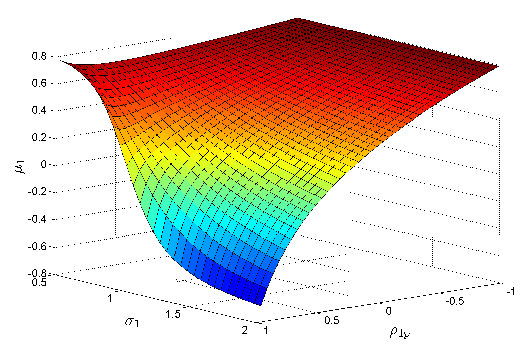
Figure 1: Expected gains for agent 1 given $\sigma_{p}=1$

2.1 Sensitivity analysis

Let us introduce the random variable $r:=p-w_{1}\xi_{1}=\sum_{k=2}^{n}w_{k}\xi_{k}$, and define

$$\sigma_{r}^{2}:=\operatorname{Var}(r),\qquad\rho_{1r}:=\frac{1}{\sigma_{1}\sigma_{r}}\operatorname{Cov}(\xi_{1},r).$$

In this section we analyze the impact on the expected payoff $\mu_{1}$ due to variations in the parameters $\sigma_{1}$, $\sigma_{r}$, and $\rho_{1r}$. Note that one has

$$\sigma_{p}^{2} =\operatorname{Var}(w_{1}\xi_{1}+r)=w_{1}^{2}\sigma_{1}^{2}+\sigma_{r}^{2}+2w_{1}\sigma_{1r}=w_{1}^{2}\sigma_{1}^{2}+\sigma_{r}^{2}+2w_{1}\sigma_{1}\sigma_{r}\rho_{1r},$$

$$\sigma_{1p} =\operatorname{Cov}(\xi_{1},w_{1}\xi_{1}+r)=w_{1}\sigma_{1}^{2}+\sigma_{1r}=w_{1}\sigma_{1}^{2}+\sigma_{1}\sigma_{r}\rho_{1r},$$

which implies, by (5),

$$\mu_{1}=\mu_{1}(\sigma_{1},\sigma_{r},\rho_{1r})=-\sqrt{2/\pi}\;\frac{w_{1}(1-w_{1})\sigma_{1}^{2}-\sigma_{r}^{2}+(1-2w_{1})\rho_{1r}\sigma_{r}\sigma_{1}}{\sqrt{(w_{1}-1)^{2}\sigma_{1}^{2}+\sigma_{r}^{2}-2(1-w_{1})\rho_{1r}\sigma_{r}\sigma_{1}}}.$$ (6)

Proposition 2.4.

The following properties of the function $\sigma_{1}\mapsto\mu_{1}(\sigma_{1},\sigma_{r},\rho_{1r})$ hold:

• it is strictly decreasing if $\rho_{1r}\leq 0$;

• if $\rho_{1r}>0$, there exists $\bar{\sigma}_{1}>0$ such that it is strictly increasing on $\left]0,\bar{\sigma}_{1}\right]$ and strictly decreasing on $\left[\bar{\sigma}_{1},\infty\right[$.

Proof.

(a) Let us write

$$\mu_{1}=-\sqrt{2/\pi}\;\frac{a\sigma_{1}^{2}+b\sigma_{1}-c}{\sqrt{\alpha\sigma_{1}^{2}-\beta\sigma_{1}+c}},$$

where

$$a :=w_{1}(1-w_{1})>0, b :=(1-2w_{1})\rho_{1r}\sigma_{r},$$

$$c :=\sigma_{r}^{2}>0, \alpha :=(1-w_{1})^{2}>0,$$

$$\beta :=2(1-w_{1})\rho_{1r}\sigma_{r}.$$

After a few tedious but straightforward calculations, one gets

$$\frac{\partial\mu_{1}}{\partial\sigma_{1}}=-\sqrt{2/\pi}\bigl{(}\alpha\sigma_{1}^{2}-\beta\sigma_{1}+c\bigr{)}^{-3/2}\,g(\sigma_{1}),$$

where

$$g(x) =a\alpha x^{3}-\frac{3}{2}a\beta x^{2}+\bigl{(}(2a+\alpha)c-b\beta/2\big{)}x+(b-\beta/2)c$$

$$=:a_{3}x^{3}+a_{2}x^{2}+a_{1}x+a_{0}$$

and

$$a_{3} =w_{1}(1-w_{1})^{3}>0,$$

$$a_{2} =-3w_{1}(1-w_{1})^{2}\sigma_{r}\rho_{1r},$$

$$a_{1} =\sigma_{r}^{2}(1-w_{1})\bigl{(}(1+2\rho_{1r}^{2})w_{1}+1-\rho_{1r}^{2}\bigr{)}>0,$$

$$a_{0} =-w_{1}\sigma_{r}^{3}\rho_{1r}.$$

It is thus immediately seen that, if $\rho_{1r}\leq 0$, then $g(x)>0$ for all $x\geq 0$, which proves (a).

(b) We are going to show that, independently of the value of $\rho_{1r}>0$, the function $g$ is strictly increasing. In fact, one has $g^{\prime}(x)=3a_{3}x^{2}+2a_{2}x+a_{1}$, whose discriminant $a_{2}^{2}-3a_{1}a_{3}$ has the same sign of $(1+w_{1})(\rho_{1r}^{2}-1)$, which is clearly negative. Therefore, $g^{\prime}(x)>0$ for all $x\geq 0$, hence $g$ is strictly increasing. In particular, since $g(0)=a_{0}<0$ and $\lim_{x\to+\infty}g(x)=+\infty$, it follows that $g$ has only one positive root $\bar{\sigma}_{1}$, with $g(x)<0$ for all $x\in\left[0,\bar{\sigma}_{1}\right[$ and $g(x)>0$ for all $x\in\left]\bar{\sigma}_{1},+\infty\right[$, which proves (b). ∎

Therefore, if the signal is negatively correlated with the aggregated signal of the others, then – ceteris paribus – a reduction in the volatility of the signal always increases the expected payoff. Our model is therefore at least partially consistent with empirical results reported in Mikhail et al. (1999), where single market participants have an incentive to acquire and process information in order to improve their forecast ability. On the other hand, it should be stressed that an improvement of the precision of the signal (i.e. a reduction of $\sigma_{1}$) does not always imply a higher expected payoff. In particular, if the signal of agent $1$ is positively correlated with the aggregated signal of all other agents, the effect of a decrease in $\sigma_{1}$ on $\mu_{1}$ depends, in a complex way, on all parameters of the model. We shall see that an analogous non-monotonic relationship holds with respect to variations in $\sigma_{r}$.

Proposition 2.5.

The following properties of the function $\sigma_{r}\mapsto\mu_{1}(\sigma_{1},\sigma_{r},\rho_{1r})$ hold:

• it is strictly increasing if $\rho_{1r}\leq 0$;

• if $\rho_{1r}>0$, there exists $\bar{\sigma}_{r}>0$ such that it is strictly decreasing on $\left]0,\bar{\sigma}_{r}\right]$ and strictly increasing on $\left[\bar{\sigma}_{r},\infty\right[$.

Proof.

Since $(\sigma_{1},\sigma_{r})\mapsto\mu_{1}(\sigma_{1},\sigma_{r})$ is homogeneous of order $1$, Euler’s theorem yields

$$\sigma_{1}\frac{\partial\mu_{1}}{\partial\sigma_{1}}(\sigma_{1},\sigma_{r})+\sigma_{r}\frac{\partial\mu_{1}}{\partial\sigma_{r}}(\sigma_{1},\sigma_{r})=\mu_{1}(\sigma_{1},\sigma_{r}),$$ (7)

hence

$$\frac{\partial\mu_{1}}{\partial\sigma_{r}} =\frac{1}{\sigma_{r}}\Bigl{(}\mu_{1}-\sigma_{1}\frac{\partial\mu_{1}}{\partial\sigma_{1}}\Bigr{)}$$

$$=\frac{\sqrt{2/\pi}}{\sigma_{r}}\bigl{(}\alpha\sigma_{1}^{2}-\beta\sigma_{1}+c\bigr{)}^{-3/2}\Bigl{(}\sigma_{1}g(\sigma_{1})-\bigl{(}a\sigma_{1}^{2}+b\sigma_{1}-c\bigr{)}\bigl{(}\alpha\sigma_{1}^{2}-\beta\sigma_{1}+c\bigl{)}\Bigr{)}$$

$$=\frac{\sqrt{2/\pi}}{\sigma_{r}}\bigl{(}\alpha\sigma_{1}^{2}-\beta\sigma_{1}+c\bigr{)}^{-3/2}\Bigl{(}(-a\beta/2-b\alpha)\sigma_{1}^{3}+\bigl{(}c(a+2\alpha)+b\beta/2\bigr{)}\sigma_{1}^{2}+$$

$$\hskip 30.00005pt-\frac{3}{2}c\beta\sigma_{1}+c^{2}\Bigr{)}$$

$$=\sqrt{2/\pi}\bigl{(}\alpha\sigma_{1}^{2}-\beta\sigma_{1}+c\bigr{)}^{-3/2}\bigl{(}\sigma_{r}^{3}+a_{1}\sigma_{1}\sigma_{r}^{2}+a_{2}\sigma_{1}^{2}\sigma_{r}+a_{3}\sigma_{1}^{3}\bigr{)}$$

$$=\sqrt{2/\pi}\bigl{(}\alpha\sigma_{1}^{2}-\beta\sigma_{1}+c\bigr{)}^{-3/2}h(\sigma_{r}),$$

where $h(x):=x^{3}+a_{1}\sigma_{1}x^{2}+a_{2}\sigma_{1}^{2}x+a_{3}\sigma_{1}^{3}$ and

$$a_{3} :=\frac{-a\beta/2-b\alpha}{\sigma_{r}}=-(1-w_{1})^{3}\rho_{1r},$$

$$a_{2} :=\frac{c(a+2\alpha)+b\beta/2}{\sigma_{r}^{2}}=w_{1}^{2}(1+2\rho_{1r}^{2})-3w_{1}(1+\rho_{1r}^{2})+2+\rho_{1r}^{2},$$

$$a_{1} :=\frac{-3c\beta/2}{\sigma_{r}^{3}}=-3(1-w_{1})\rho_{1r}.$$

Let us first show that $a_{2}>0$: in fact, looking at the above definition of $a_{2}$ as a polynomial in $w_{1}$, its roots are

$$\frac{3(1+\rho_{1r}^{2})\pm(1-\rho_{1r}^{2})}{2+4\rho_{1r}^{2}}\geq 1.$$

(a) Since $a_{1},a_{2},a_{3}>0$, Descartes’ rule of signs implies that $h$ has no positive roots. Moreover, since $h(0)=\sigma_{1}^{3}a_{3}>0$, we conclude that $h(x)>0$ for all $x>0$, i.e. $\partial\mu_{1}/\partial\sigma_{r}>0$.

(b) Note that $h$ is strictly increasing: in fact, one has $h^{\prime}(x)=3x^{2}+2a_{1}\sigma_{1}x+a_{2}\sigma_{1}^{2}$, and the discriminant of this polynomial is proportional to

$$a_{1}^{2}-3a_{2}=3(1-\rho_{1r}^{2})(1-w_{1})(w_{1}-2)<0.$$

Since $a_{3}<0$ implies that $h(0)<0$, we conclude that $h$ admits exactly one positive root $\bar{\sigma}_{r}$, as well as that $h$ is negative on $[0,\bar{\sigma}_{r}]$ and positive on $\left]\bar{\sigma}_{r},+\infty\right[$. ∎

Note that the first statement of the previous Proposition simply says that, if $\rho_{1r}\leq 0$, the expected payoff $\mu_{1}$ improves as $\sigma_{r}$ increases, i.e. agent $1$ obtains a higher payoff as the relative accuracy of his own signal improves. On the other hand, if $\rho_{1r}>0$, in analogy to Proposition 2.4, the relationship between $\mu_{1}$ and $\sigma_{r}$ is no longer monotonic and is determined in a complex way by all parameters of the model. This $J$-shaped relationship between forecast precision and trading profitability was first reported in simulation studies by Schredelseker (1984, 2001) and also documented in experimental works by Huber (2007) and Huber et al. (2008). The authors use a cumulative information setting which implies a positive pairwise correlation. In the numerical example of Section 4 we adopt this setting, thus reproducing the behavior observed in the above mentioned papers.

It should be remarked that, even though Propositions 2.4 and 2.5 are qualitatively very similar, it is not true in general that $\partial\mu_{1}/\partial\sigma_{1}(\sigma_{1},\sigma_{r})>0$ implies $\partial\mu_{1}/\partial\sigma_{r}(\sigma_{1},\sigma_{r})<0$ for all $\sigma_{1}$, $\sigma_{r}$, as it can be immediately realized looking at (7). More precise information on the values of the parameters determining the signs of $\mu_{1}$ and of its partial derivatives can be easily obtained.

Proposition 2.6.

Let $\sigma_{1}$, $\sigma_{r}$ be fixed positive constants, and $\alpha_{+}=\alpha_{+}(\rho_{1r})$ be defined as in (8) below. The function $\rho_{1r}\mapsto\mu_{1}(\sigma_{1},\sigma_{r},\rho_{1r})$ is locally decreasing if $\sigma_{r}<\alpha_{+}\sigma_{1}$ and locally increasing if $\sigma_{r}>\alpha_{+}\sigma_{1}$.

Proof.

One has, setting $\alpha:=\sigma_{r}/\sigma_{1}$,

$$\frac{\partial\mu_{1}}{\partial\rho_{1r}} =\sqrt{2/\pi}\,A^{-3}\Bigl{[}(1-w_{1})(1-2w_{1})\sigma_{1}^{2}\sigma_{r}^{2}\rho+w_{1}\sigma_{1}\sigma_{r}^{3}-(1-w_{1})^{3}\sigma_{1}^{3}\sigma_{r}\Bigr{]}$$

$$=\sqrt{2/\pi}\,A^{-3}\sigma_{1}^{3}\sigma_{r}\Bigl{[}w_{1}\alpha^{2}+(1-w_{1})(1-2w_{1})\rho_{1r}\alpha-(1-w_{1})^{3}\Bigr{]},$$

where $A$ denotes the denominator of the fraction appearing in (6). Then the sign of $\partial\mu_{1}/\partial\rho_{1r}$ is equal to the sign of the polynomial in $\alpha$

$$w_{1}\alpha^{2}+(1-w_{1})(1-2w_{1})\rho_{1r}\alpha-(1-w_{1})^{3},$$

whose roots $\alpha_{-}<0<\alpha_{+}$ are

$$\alpha_{\pm}:=(1-w_{1})\frac{-(1-2w_{1})\rho_{1r}\pm\sqrt{(1-2w_{1})^{2}\rho_{1r}^{2}+4w_{1}(1-w_{1})}}{2w_{1}}.$$ (8)

In particular, if $\sigma_{r}/\sigma_{1}<\alpha_{+}$, then $\partial\mu_{1}/\partial\rho_{1r}$ is negative; if $\sigma_{r}/\sigma_{1}>\alpha_{+}$, then $\partial\mu_{1}/\partial\rho_{1r}$ is positive. ∎

Corollary 2.7.

Let $\sigma_{1}$, $\sigma_{r}>0$ be given, and define

$$\ell :=\frac{1-w_{1}}{2w_{1}}\Bigl{(}\sqrt{(1-2w_{1})^{2}+4w_{1}(1-w_{1})}-\lvert 1-2w_{1}\rvert\Bigr{)},$$

$$u :=\frac{1-w_{1}}{2w_{1}}\Bigl{(}\sqrt{(1-2w_{1})^{2}+4w_{1}(1-w_{1})}+\lvert 1-2w_{1}\rvert\Bigr{)}.$$

If $\sigma_{r}/\sigma_{1}\in[\ell,u]$, then

• if $w_{1}<1/2$, then there exists $\bar{\rho}$ such that $\rho_{1r}\mapsto\mu_{1}(\rho_{1r})$ is decreasing on $[-1,\bar{\rho}]$ and increasing on $[\bar{\rho},1]$;

• if $w_{1}>1/2$, then there exists $\bar{\rho}$ such that $\rho_{1r}\mapsto\mu_{1}(\rho_{1r})$ is increasing on $[-1,\bar{\rho}]$ and decreasing on $[\bar{\rho},1]$;

Otherwise, if $\sigma_{r}/\sigma_{1}<\ell$, then $\rho_{1r}\mapsto\mu_{1}(\rho_{1r})$ is decreasing on $[-1,1]$; if $\sigma_{r}/\sigma_{1}>u$, then $\rho_{1r}\mapsto\mu_{1}(\rho_{1r})$ is increasing on $[-1,1]$.

Proof.

Note that one has

$$\frac{\partial\alpha_{+}}{\partial\rho_{1r}}=\frac{1-w_{1}}{2w_{1}}\,\frac{-a\sqrt{a^{2}\rho_{1r}^{2}+b}+a^{2}\rho_{1r}}{\sqrt{a^{2}\rho_{1r}^{2}+b}},$$

where

$$a:=1-2w_{1},\qquad b:=4w_{1}(1-w_{1})>0,$$

therefore $\partial\alpha_{+}/\partial\rho_{1r}>0$ if and only if

$$a^{2}\rho_{1r}>a\sqrt{a^{2}\rho_{1r}^{2}+b}.$$

Simple calculations immediately reveal that this inequality is always satisfied if $a=1-2w_{1}<0$, and never satisfied if $a=1-2w_{1}>0$. Equivalently, $\rho_{1r}\mapsto\alpha_{+}(\rho_{1r})$ is increasing if $w_{1}>1/2$, and decreasing if $w_{1}<1/2$. To complete the proofs it is enough to observe that one has

$$\alpha_{+}(-1) =\frac{1-w_{1}}{2w_{1}}\Bigl{(}(1-2w_{1})+\sqrt{(1-2w_{1})^{2}+4w_{1}(1-w_{1})}\Bigr{)}$$

$$\alpha_{+}(1) =\frac{1-w_{1}}{2w_{1}}\Bigl{(}-(1-2w_{1})+\sqrt{(1-2w_{1})^{2}+4w_{1}(1-w_{1})}\Bigr{)}.\qed$$

To describe the relationship between the expect payoff of agent $1$ and the correlation coefficient $\rho_{1r}$ we can thus distinguish three regimes: if the relative accuracy of his signal is low ($\sigma_{r}/\sigma_{1}<\ell$), then, for any $\rho_{ir}\in[-1,1]$, agent $1$ gains from a decline in the correlation between his signal and the aggregated signal of all other agents; if the relative accuracy of his signal is high ($\sigma_{r}/\sigma_{1}>u$), then, for any $\rho_{ir}\in[-1,1]$, agent 1 gains from an increase in correlation; if the (inverse) relative accuracy $\sigma_{r}/\sigma_{1}$ falls within the interval $[\ell,u]$, then the dependence of $\mu_{1}$ on $\rho_{1r}$ turns out to be non-monotonic. In the first two cases, i.e. when the (inverse) relative accuracy $\sigma_{r}/\sigma_{1}$ falls above $u$ or below $\ell$, the result can be heuristically motivated as follows: if agent 1 overestimates (underestimates) the true value, then the market price will be even higher (lower) than his signal. According to his decision rule (buying when the signal is above the market price and selling when the signal is below the market price), he will then take the correct trading position. Moreover, note that, in the third regime, if $w_{1}<1/2$ the function $\rho_{1r}\mapsto\mu_{1}(\rho_{1r})$ has exactly one global minimum, which implies a higher expected payoff for extreme (either positive or negative) rather than for intermediate levels of correlation. This result hence offers a complete explanation of the contradicting empirical observations according to which analysts with a high reputation tend to herd (see, e.g. Graham, 1999), as well as to deviate more drastically from the consensus forecast (see, e.g., Lamont, 2002; Bernhardt et al., 2006).

2.2 Full Communication Equilibrium

In Section 2.1 we consider naive investors who trade on the basis of their individual signals. We propose a one-period model where the true value of the firm, and therefore gains and losses of each analyst, are revealed immediately after the trade. Of course, in the long run the different agents will participate to the market only under the condition that the expected payoff is not negative. This holds also for the market marker, whose expected payoff – by definition of a dealer market – is given by the negative sum of the single $\mu_{i}$’s. In order to avoid a breakdown of trading as described by the theory of lemon markets and given the zero-sum property of the game, an equilibrium implies that the expected payoff of each agent must be equal to zero (i.e, $\mu_{i}=0$ $\forall i=1,\ldots,n$). A natural question is whether our model, where prices are equal to a weighted average of the single signals, see (1), is able to accommodate such an equilibrium.

In order to keep the market alive, the market maker will have an interest to ensure a level playing field for all participants. He could use the observed covariance matrix $Q$ and the single signals $\xi_{i}$ revealed by the conditional orders to set the price. Using the model of Black and Litterman (1992) with non-informative priors, one obtains the following choice for the price: $p^{*}:=\langle Q^{-1}\mathbf{1},\mathbf{1}\rangle^{-1}\langle Q^{-1}\mathbf{1},\xi\rangle$, which corresponds in (1) to

$$w^{*}:=\langle Q^{-1}\mathbf{1},\mathbf{1}\rangle^{-1}(Q^{-1}\mathbf{1}).$$ (9)

If market prices are fully revealing all available information, then the market is said to be in a full communication equilibrium (see Radner, 1979). With this choice of $w$ one has, for any $k\in\{1,2,\ldots,n\}$,

$$\sigma_{kp}=\langle Q_{k},w^{*}\rangle=\frac{\langle Q^{-1}Q_{1},\mathbf{1}\rangle}{\langle Q^{-1}\mathbf{1},\mathbf{1}\rangle}=\frac{\langle e_{k},\mathbf{1}\rangle}{\langle Q^{-1}\mathbf{1},\mathbf{1}\rangle}=\frac{1}{\langle Q^{-1}\mathbf{1},\mathbf{1}\rangle}=\langle Qw^{*},w^{*}\rangle=\sigma_{p}^{2},$$

hence, by (5), in equilibrium the expected payoff of all market participants is zero. As a consequence, the expected payoff of the market marker is also equal to zero. According to Radner (1979) any fully-revealing communication equilibrium is also a fully-revealing rational expectation equilibrium. Let us show that, in fact, such equilibrium is unique, in the sense of the following Proposition.

Proposition 2.8.

There exists one and only one vector $w\in\mathbb{R}^{n}$, with $\sum_{k=1}^{n}w_{k}=1$, such that $\mu_{i}=0$ for all $i=1,2,\ldots,n$.

Proof.

It is enough to show that there exists a unique vector $w\in\mathbb{R}^{n}$ with $\sum_{k=1}^{n}w_{k}=1$, such that

$$\langle Qw,w\rangle=\langle Q_{k},w\rangle\qquad\forall k=1,\ldots,n.$$ (10)

Existence has already been proved by explicitly constructing a solution $w^{*}$. It is thus enough to prove uniqueness. Condition (10) implies $\langle Q_{1},w\rangle=\langle Q_{k},w\rangle$ for all $k>1$, hence $\langle Q_{1}-Q_{k},w\rangle=0$ for all $k>1$. This in turn implies $w\in V^{\perp}$, where

$$V=\operatorname{span}(Q_{1}-Q_{2},\ldots,Q_{1}-Q_{n}),$$

and $V^{\perp}$ stands for the orthogonal complement of $V$ in $\mathbb{R}^{n}$, so that $\mathbb{R}^{n}=V\oplus V^{\perp}$. Since $Q$ is assumed to be non-singular, the vectors $Q_{1},\ldots,Q_{n}$ are linearly independent, hence $\dim V=n-1$, which implies that $\dim V^{\perp}=1$. Since $w^{*}\neq 0$, then $w^{*}$ is a generator of $V^{\perp}$. In particular, $0\neq w\in V^{\perp}$ implies that there exists $\alpha\neq 0$ such that $w=\alpha w^{*}$. Then $1=\sum_{k=1}^{n}w_{k}=\alpha\sum_{k=1}^{n}w^{*}_{k}=\alpha$ yields the uniqueness of $w^{*}$. ∎

3 Density function of the payoff

In the previous section we have presented a closed-form solution for the expected trading payoffs of the single agents, see (5). As a matter of fact, we can give a complete characterization of trading payoffs as random variables. In this section we provide a closed-form expression for the density of the payoff for each agent. Throughout the section we adopt the notation introduced in Lemma 2.1 and Proposition 2.2.

We begin with an auxiliary result, which might be interesting in its own right.

Proposition 3.1.

Let

$$F(x_{1},x_{2}):=\mathbb{P}\bigl{(}p\leq x_{1},\,\operatorname{sgn}(\xi_{1}-p)=x_{2}\bigr{)},\qquad x_{1}\in\mathbb{R},\;x_{2}\in\{-1,1\},$$

denote the joint distribution of $p$ and $\operatorname{sgn}(\xi_{1}-p)$. One has

$$F(x_{1},x_{2};\beta)=\Phi(x_{1}/c)\Phi(-\beta x_{1}x_{2}/c)-\frac{x_{2}}{2\pi}\arctan(1/\beta)+x_{2}\operatorname{sgn}\beta\biggl{(}\frac{1}{4}+\int_{0}^{\frac{|\beta|}{c}x_{1}}\Phi(z/|\beta|)\phi(z)\,dz\biggr{)}.$$

Proof.

By Lemma 2.1, there exist $a>0$, $b\in\mathbb{R}$ and $c>0$ such that $p=cY$ and $\xi_{1}=aX+bY$ in law, where $X$ and $Y$ are independent standard Gaussian random variables. Setting $\beta=(c-b)/a$, one has

$$F(x_{1},x_{2})=\mathbb{P}\bigl{(}Y\leq x_{1}/c,\;\operatorname{sgn}(X-\beta Y)=x_{2}\bigr{)}.$$

Let us record, for later use, the following obvious observation:

$$\Phi(x_{1}/c) =\mathbb{P}(Y\leq x_{1}/c)=\mathbb{P}\bigl{(}Y\leq x_{1}/c,\,\operatorname{sgn}(X-\beta Y)=-1\bigr{)}+\mathbb{P}\bigl{(}Y\leq x_{1}/c,\,\operatorname{sgn}(X-\beta Y)=1\bigr{)}$$

$$=F(x_{1},-1)+F(x_{1},1).$$

Let us consider first the case $\beta>0$: one has

$$F(x_{1},-1)=\mathbb{P}\bigl{(}Y\leq x_{1}/c,\,\operatorname{sgn}(X-\beta Y)=-1\bigr{)}=\mathbb{P}\bigl{(}Y\leq x_{1}/c,\,X<\beta Y\bigr{)},$$

where we have used the fact that $a>0$, $c>0$. Hence

$$F(x_{1},-1) =\mathbb{P}\bigl{(}X/\beta\leq Y\leq x_{1}/c\bigr{)}$$

$$=\int_{-\infty}^{\frac{\beta}{c}x_{1}}\mathbb{P}(z/\beta\leq Y\leq x_{1}/c)\,\phi(z)\,dz$$

$$=\Phi(x_{1}/c)\Phi(\beta x_{1}/c)-\int_{-\infty}^{\frac{\beta}{c}x_{1}}\Phi(z/\beta)\phi(z)\,dz.$$

Appealing to Lemma A.1, we end up with

$$F(x_{1},-1)=\Phi(x_{1}/c)\Phi(\beta x_{1}/c)-\frac{1}{4}+\frac{1}{2\pi}\arctan(1/\beta)-\int_{0}^{\frac{\beta}{c}x_{1}}\Phi(z/\beta)\phi(z)\,dz.$$

The expression for $F(x_{1},1)$ is obtained as follows:

$$F(x_{1},1) =\Phi(x_{1}/c)-F(x_{1},-1)$$

$$=\Phi(x_{1}/c)\bigl{(}1-\Phi(\beta x_{1}/c)\bigr{)}+\frac{1}{4}-\frac{1}{2\pi}\arctan(1/\beta)+\int_{0}^{\frac{\beta}{c}x_{1}}\Phi(z/\beta)\phi(z)\,dz$$

$$=\Phi(x_{1}/c)\Phi(-\beta x_{1}/c)+\frac{1}{4}-\frac{1}{2\pi}\arctan(1/\beta)+\int_{0}^{\frac{\beta}{c}x_{1}}\Phi(z/\beta)\phi(z)\,dz$$

Let us now consider the case $\beta<0$: by a reasoning completely analogous to the one used above, we can write

$$F(x_{1},1) =\mathbb{P}\bigl{(}Y\leq x_{1}/c,\;X/\beta\leq Y\bigr{)}=\mathbb{P}(X/\beta\leq Y\leq x_{1}/c)$$

$$=\int_{\frac{\beta}{c}x_{1}}^{\infty}\mathbb{P}(z/\beta\leq Y\leq x_{1}/c)\,\phi(z)\,dz$$

$$=\Phi(x_{1}/c)\Phi(-\beta x_{1}/c)-\int_{-\infty}^{-\frac{\beta}{c}x_{1}}\Phi(-z/\beta)\phi(z)\,dz$$

$$=\Phi(x_{1}/c)\Phi(-\beta x_{1}/c)-\frac{1}{4}-\frac{1}{2\pi}\arctan(1/\beta)-\int_{0}^{\frac{|\beta|}{c}x_{1}}\Phi(z/|\beta|)\phi(z)\,dz,$$

hence also

$$F(x_{1},-1) =\Phi(x_{1}/c)-F(x_{1},1)$$

$$=\Phi(x_{1}/c)\bigl{(}1-\Phi(-\beta x_{1}/c)\bigr{)}+\frac{1}{4}+\frac{1}{2\pi}\arctan(1/\beta)+\int_{0}^{\frac{|\beta|}{c}x_{1}}\Phi(z/|\beta|)\phi(z)\,dz$$

$$=\Phi(x_{1}/c)\Phi(\beta x_{1}/c)+\frac{1}{4}+\frac{1}{2\pi}\arctan(1/\beta)+\int_{0}^{\frac{|\beta|}{c}x_{1}}\Phi(z/|\beta|)\phi(z)\,dz.$$

We may thus write

$$F(x_{1},-1) =\Phi(x_{1}/c)\Phi(\beta x_{1}/c)+\frac{1}{2\pi}\arctan(1/\beta)-\operatorname{sgn}\beta\left(\frac{1}{4}+\int_{0}^{\frac{|\beta|}{c}x_{1}}\Phi(z/\beta)\phi(z)\,dz\right),$$

$$F(x_{1},1) =\Phi(x_{1}/c)\Phi(-\beta x_{1}/c)-\frac{1}{2\pi}\arctan(1/\beta)+\operatorname{sgn}\beta\left(\frac{1}{4}+\int_{0}^{\frac{|\beta|}{c}x_{1}}\Phi(z/\beta)\phi(z)\,dz\right),$$

that are equivalent to the claim. ∎

Remark 3.2.

The joint distribution of $p$ and $\operatorname{sgn}(\xi_{1}-p)$ can alternatively be expressed in terms of the bivariate Gaussian law. Consider, for instance, the case $\beta>0$ and $x_{2}=-1$: Lemma A.2 yields

$$F(x_{1},-1) =\Phi(x_{1}/c)\Phi(\beta x_{1}/c)-\int_{-\infty}^{\frac{\beta}{c}x_{1}}\Phi(z/\beta)\phi(z)\,dz$$

$$=\Phi(x_{1}/c)\Phi(\beta x_{1}/c)-\Phi_{2}\left(\beta x_{1}/c,0;-\frac{1}{\sqrt{1+\beta^{2}}}\right),$$

where $\Phi_{2}(\cdot,\cdot;\rho)$ denotes the distribution function of a bivariate Gaussian random variable with correlation coefficient $\rho$.

The following Proposition is the main result of this section and of the whole paper.

Proposition 3.3.

Let $M=p\operatorname{sgn}(\xi_{1}-p)$ denote the negative payoff of agent $1$. The random variable $M$ has a (smooth) density $f_{M}$ given by

$$f_{M}(z)=\frac{2}{c}\phi(z/c)\Phi(-\beta z/c).$$

Proof.

Let us first compute the distribution $F_{M}(z):=\mathbb{P}(M\leq z)$ of the random variable $M$. One has

$$F_{M}(z) =\mathbb{P}(p\operatorname{sgn}(\xi_{1}-p)\leq z)$$

$$=\mathbb{P}\bigl{(}p\operatorname{sgn}(\xi_{1}-p)\leq z,\;\operatorname{sgn}(\xi_{1}-p)=-1\bigr{)}+\mathbb{P}\bigl{(}p\operatorname{sgn}(\xi_{1}-p)\leq z,\;\operatorname{sgn}(\xi_{1}-p)=1\bigr{)}$$

$$=\mathbb{P}\bigl{(}p\geq-z,\;\operatorname{sgn}(\xi_{1}-p)=-1\bigr{)}+\mathbb{P}\bigl{(}p\leq z,\;\operatorname{sgn}(\xi_{1}-p)=1\bigr{)}$$

$$=\mathbb{P}(\operatorname{sgn}(\xi_{1}-p)=-1)-F(-z,-1)+F(z,1),$$

where $F$ denotes the joint distribution of $p$ and $\operatorname{sgn}(\xi_{1}-p)$, and

$$\mathbb{P}(\operatorname{sgn}(\xi_{1}-p)=-1)=\mathbb{P}(X\leq\beta Y)=1/2,$$

which follows immediately because $X$ and $Y$ are independent, symmetric, and have a continuous distribution: $\mathbb{P}(X\leq\beta Y)+\mathbb{P}(X\geq\beta Y)=1$, but $\mathbb{P}(X\geq\beta Y)=\mathbb{P}(-X\geq-\beta Y)=\mathbb{P}(X\leq\beta Y)$.

Thanks to Proposition 3.1, one has

$$F_{M}(z)=C_{\beta}+\bigl{(}2\Phi(z/c)-1\bigr{)}\Phi(-\beta z/c)+\operatorname{sgn}\beta\left(\int_{0}^{-\frac{|\beta|}{c}z}\Phi(y/|\beta|)\phi(y)\,dy+\int_{0}^{\frac{|\beta|}{c}z}\Phi(y/|\beta|)\phi(y)\,dy\right),$$

where $C_{\beta}$ denotes a constant that depends only on $\beta$, hence

$$f_{M}(z)=\frac{d}{dz}F_{M}(z) =\frac{2}{c}\phi(z/c)\Phi(-\beta z/c)-\frac{\beta}{c}\phi(\beta z/c)\bigl{(}2\Phi(z/c)-1\bigr{)}$$

$$\qquad+\operatorname{sgn}\beta\,\Bigl{(}\frac{|\beta|}{c}\Phi(z/c)\phi(|\beta|z/c)-\frac{|\beta|}{c}\Phi(-z/c)\phi(-|\beta|z/c)\Bigr{)}$$

$$=\frac{2}{c}\phi(z/c)\Phi(-\beta z/c)+\frac{\beta}{c}\phi(\beta z/c)-2\frac{\beta}{c}\Phi(z/c)\phi(\beta z/c)$$

$$\qquad+\frac{\beta}{c}\Phi(z/c)\phi(\beta z/c)-\frac{\beta}{c}\Phi(-z/c)\phi(\beta z/c)$$

$$=\frac{2}{c}\phi(z/c)\Phi(-\beta z/c)+\frac{\beta}{c}\phi(\beta z/c)-\frac{\beta}{c}\phi(\beta z/c)\bigl{(}\Phi(z/c)+\Phi(-z/c)\bigr{)}$$

$$=\frac{2}{c}\phi(z/c)\Phi(-\beta z/c).\qed$$

It is immediately seen that the density of the random variable $-M$, which represents the trading payoff of agent $1$, is given by

$$f_{-M}(z)=f_{M}(-z)=\frac{2}{c}\phi(z/c)\Phi(\beta z/c).$$

3.1 Higher moments

Given the complete probabilistic characterization of the (negative) trading profit $M$ just obtained, one can compute any moment of $M$ simply integrating against the density $f_{M}$. It is easier, however, to proceed differently.

For an odd number $2k-1$, $k\in\mathbb{N}$, we define $(2k-1)!!:=\prod_{j=1}^{k}(2j-1)$, and set, by convention, $(-1)!!:=1$.

Proposition 3.4.

Let $k\in\mathbb{N}$. One has

$$\mathop{{}\mathbb{E}}M^{2k} =(2k-1)!!\,\langle Qw,w\rangle^{k},$$

$$\mathop{{}\mathbb{E}}M^{2k-1} =-\frac{2^{k}(k-1)!\,c^{2k-1}\beta}{\sqrt{2\pi(1+\beta^{2})}}\,\sum_{j=0}^{k-1}\frac{(2j-1)!!}{(2j)!!}\,\frac{1}{(1+\beta^{2})^{j}}.$$

Proof.

Since $M^{2k}=p^{2k}$, and $p=\langle w,\xi\rangle$ is a centered Gaussian random variable with variance $\langle Qw,w\rangle$, standard formulas for moments of Gaussian laws give

$$\mathop{{}\mathbb{E}}M^{2k}=\mathop{{}\mathbb{E}}p^{2k}=\mathop{{}\mathbb{E}}\langle w,\xi\rangle^{2k}=(2k-1)!!\,\langle Qw,w\rangle^{k}.$$

Moreover, by Lemma 2.1, one has

$$\mathop{{}\mathbb{E}}M^{2k+1} =\mathop{{}\mathbb{E}}p^{2k+1}\operatorname{sgn}(\xi_{1}-p)=c^{2k+1}\mathop{{}\mathbb{E}}Y^{2k+1}\operatorname{sgn}(X-\beta Y)$$

$$=c^{2k+1}\int_{\mathbb{R}}y^{2k+1}\mathop{{}\mathbb{E}}\left[\operatorname{sgn}(X-\beta y)\right]\,\phi(y)\,dy,$$

where $\mathop{{}\mathbb{E}}\left[\operatorname{sgn}(X-\beta y)\right]=1-2\Phi(\beta y)$, hence

$$\mathop{{}\mathbb{E}}M^{2k+1}=-2c^{2k+1}\int_{\mathbb{R}}y^{2k+1}\Phi(\beta y)\,\phi(y)\,dy.$$ (11)

Note that, setting $v(y)=y^{2k}\phi(y)$, one has

$$v^{\prime}(y)=\bigl{(}2ky^{2k-1}-y^{2k+1}\bigr{)}\phi(y),$$

hence, integrating by parts in (11),

$$\begin{split}\int_{\mathbb{R}}\Phi(\beta y)\,y^{2k+1}\phi(y)\,dy&=\int_{\mathbb{R}}\Phi(\beta y)\bigl{(}y^{2k+1}-2ky^{2k-1}\bigr{)}\phi(y)\,dy\\ &\qquad+2k\int_{\mathbb{R}}\Phi(\beta y)\,y^{2k-1}\phi(y)\,dy\\ &=\beta\int_{\mathbb{R}}y^{2k}\phi(\beta y)\phi(y)\,dy+2k\int_{\mathbb{R}}\Phi(\beta y)\,y^{2k-1}\phi(y)\,dy,\end{split}$$ (12)

where, setting $\sigma_{\beta}:=(1+\beta^{2})^{-1/2}$ for convenience of notation, and recalling again standard formulas for moments of Gaussian laws,

$$\int_{\mathbb{R}}y^{2k}\phi(\beta y)\phi(y)\,dy =\bigl{(}2\pi(1+\beta^{2})\bigr{)}^{-1/2}\frac{1}{\sigma_{\beta}\sqrt{2\pi}}\int_{\mathbb{R}}y^{2k}e^{-y^{2}/(2\sigma_{\beta}^{2})}\,dy$$

$$=\bigl{(}2\pi(1+\beta^{2})\bigr{)}^{-1/2}\,(2k-1)!!\,(1+\beta^{2})^{-k}.$$

Therefore, setting

$$f_{k} :=\int_{\mathbb{R}}\Phi(\beta y)\,y^{2k-1}\phi(y)\,dy,$$

$$a_{k} :=\frac{\beta}{\sqrt{2\pi(1+\beta^{2})}}\,(2k-1)!!\,(1+\beta^{2})^{-k},$$

(12) can be written as

$$f_{k+1}-2kf_{k}=a_{k},\qquad f_{1}=\frac{\beta}{\sqrt{2\pi(1+\beta^{2})}}.$$

Dividing both sides of this difference equation by $2^{k}k!$, we are left with

$$\frac{f_{k+1}}{2^{k}\,k!}-\frac{f_{k}}{2^{k-1}\,(k-1)!}=\frac{a_{k}}{2^{k}\,k!},$$

hence, setting

$$g_{k}:=\frac{f_{k}}{2^{k-1}\,(k-1)!},\qquad b_{k}:=\frac{a_{k}}{2^{k}\,k!},$$

the previous difference equation is equivalent to

$$g_{k+1}-g_{k}=b_{k},\qquad g_{1}=\frac{\beta}{\sqrt{2\pi(1+\beta^{2})}},$$

which can be easily solved, writing the telescoping sum

$$g_{k}-g_{1} =(g_{k}-g_{k-1})+(g_{k-1}-g_{k-2})+\cdots+(g_{2}-g_{1})$$

$$=b_{k-1}+b_{k-2}+\cdots+b_{1},$$

which yields

$$f_{k} =2^{k-1}(k-1)!\,g_{k}=2^{k-1}(k-1)!\,\biggl{(}g_{1}+\sum_{j=1}^{k-1}b_{j}\biggl{)}$$

$$=2^{k-1}(k-1)!\,\biggl{(}\frac{\beta}{\sqrt{2\pi(1+\beta^{2})}}+\frac{\beta}{\sqrt{2\pi(1+\beta^{2})}}\sum_{j=1}^{k-1}\frac{(2j-1)!!}{2^{j}j!}\,\frac{1}{(1+\beta^{2})^{j}}\biggr{)}$$

$$=\frac{2^{k-1}(k-1)!\,\beta}{\sqrt{2\pi(1+\beta^{2})}}\,\sum_{j=0}^{k-1}\frac{(2j-1)!!}{(2j)!!}\,\frac{1}{(1+\beta^{2})^{j}}.$$

By definition of $f_{k}$ and (11) one finally obtains

$$\mathop{{}\mathbb{E}}M^{2k-1}=-2c^{2k-1}f_{k}=-\frac{2^{k}(k-1)!\,c^{2k-1}\beta}{\sqrt{2\pi(1+\beta^{2})}}\,\sum_{j=0}^{k-1}\frac{(2j-1)!!}{(2j)!!}\,\frac{1}{(1+\beta^{2})^{j}}.\qed$$

It is immediately seen that the moments of the payoff $-M$ of even degree coincide with those of $M$, while the moments of odd degree are equal in absolute value, but with opposite sign. Moreover, centered moments can easily be obtained by the non-central one just derived.

4 Numerical example

In this section we illustrate our main results with a numerical example. We assume that four agents, labeled by $i\in\{1,\ldots,4\}$, participate to the market. The covariance matrix $Q$ of their signals is displayed in Table 1 below. The analysts are labeled according to their forecast precision (measured by the standard deviation $\sigma_{i}$ of their signals), in reverse order. The market maker assigns equal weight ($w_{i}=0.25)$ to each signal. The numerical values chosen here try to mimic models with a cumulative information structure (see Schredelseker, 1984, 2001), where analysts with an intermediate accuracy implicitly face the highest correlation (note that the signal of agent $1$ is less correlated with other agents’ signals than the signal of agent $2$).

$i$	$\sigma_{i}$	$C$				$Q$
1	1.3	1	0.9	0.6	0.3	1.690	1.404	0.858	0.390
2	1.2	0.9	1	0.8	0.6	1.404	1.440	1.056	0.720
3	1.1	0.6	0.8	1	0.7	0.858	1.056	1.210	0.770
4	1	0.3	0.6	0.7	1	0.390	0.720	0.770	1.000

Table 1: Signal structure of the numerical example: $C$ and $Q$ denote the correlation matrix and the covariance matrix, respectively.

In the following we compare the payoffs of all analysts. We use the formulas of the previous section to calculate the first four central moments. Table 2 shows that, although analyst $1$ has a less accurate signal than analyst $2$ (with a resulting higher variance and kurtosis in the payoffs), his expected payoff is better. Obviously, analyst $2$ suffers from his high correlation with all other market participants, which is also reflected in a more negative skewness.

Therefore, our model reproduces the non-monotone relationship between forecast precision and trading profitability observed in Schredelseker (1984, 2001).

$i$	$\mu_{i}$	$\sigma^{2}_{i}$	$\varsigma_{i}$	$\kappa_{i}$
1	-0.115	0.970	-0.001	2.825
2	-0.406	0.819	-0.029	2.018
3	0.016	0.983	0.000	2.900
4	0.285	0.902	0.010	2.444

Table 2: Higher moments of the payoff for analysts $i=1,\ldots,4$: $\varsigma_{i}$ and $\kappa_{i}$ denote the skewness and kurtosis of agent $i$, respectively.

Figure 2 shows the density function of the payoff for all analysts.

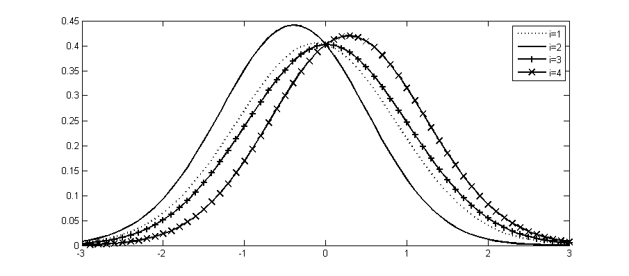
Figure 2: Density function for the payoffs of analysts $i=1,\ldots,4$.

Figure 3 shows the dependence of the expected payoff of agent $1$ on the accuracy of his own signal (as measured by the standard deviation $\sigma_{1}$) and on the correlation between his signal $\xi_{1}$ and the aggregated signal of all other agents $r$. The value of $\sigma_{r}$ is equal to $0.739$. The non-monotonic relationship between $\mu_{1}$ and $\sigma_{1}$ is clearly displayed for some positive values of $\rho_{1r}$. Moreover, while for large (small) values of $\sigma_{1}$ the expected payoff is decreasing (increasing) as $\rho_{1r}$ increases, for intermediate values of $\sigma_{1}$ a non-monotonic behaviour can be observed. Given $w_{1}=0.25<1/2$, $\mu_{1}$ is first decreasing and then increasing in $\rho_{1r}$.

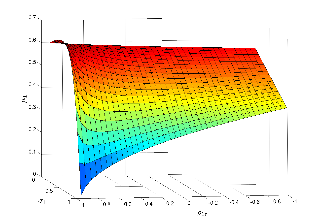
Figure 3: Expected payoff of analysts $1$ as function of $\sigma_{1}$ and $\rho_{1r}$, with $\sigma_{r}=0.739$.

5 Conclusion

We propose a model in which analysts differ in the precision of their signals as well as in the correlation between each other. We provide a complete characterization of the trading payoff of each agent, obtaining its probability density function in closed form, as well as explicit expressions for its moments of all orders. Such precise description allows us to perform a detailed sensitivity analysis, with the following implications: If the forecasts of an analyst are negatively correlated with the aggregated forecasts of the others, then he always takes advantage of improving his forecast skills. If the correlation between the forecasts is positive, then a non-monotonic relationship between forecast precision and trading profitability exists. Furthermore, the impact of correlation on the expected payoff of an analyst depends on the relative accuracy of his signal: if the relative accuracy is below (above) a certain threshold, then he suffers (benefits) from an increasing correlation, while for intermediate levels of relative accuracy the relationship is non-monotonic.

This is the first time, to the best of our knowledge, that an analytical model is proposed, which fully explains the non-trivial interplay between forecast accuracy and trading performance. Our model recovers as special cases previous (partial) results from simulation studies, and is able to explain the different – sometimes contradicting – empirical observations reported in the literature. Finally, we provide strong evidence that empirical studies on the relationship between forecast precision and trading profitability need to take into account the correlation structure of the forecasts.

Appendix A Appendix

Lemma A.1.

Let $a\in\mathbb{R}$. One has

$$\int_{0}^{\infty}\Phi(ax)\,\phi(x)\,dx =\frac{1}{4}+\frac{1}{2\pi}\arctan a,$$

$$\int_{-\infty}^{0}\Phi(ax)\,\phi(x)\,dx =\frac{1}{4}-\frac{1}{2\pi}\arctan a.$$

Proof.

For $a>0$ one has

$$\Phi(ax)=\frac{1}{2}+\int_{0}^{ax}\phi(y)\,dy\qquad\forall x\geq 0,$$

hence

$$\int_{0}^{\infty}\Phi(ax)\,\phi(x)\,dx=\int_{0}^{\infty}\left(\frac{1}{2}+\int_{0}^{ax}\phi(y)\,dy\right)\phi(x)\,dx=\frac{1}{4}+\int_{D_{a}}\phi_{2}(x,y)\,dx\,dy,$$

where $\mathbb{R}^{2}\supset D_{a}:=\bigl{\{}0\leq x<\infty,\;0\leq y\leq ax\bigr{\}}$ and $\phi_{2}$ stands for the density of the standard Gaussian measure on $\mathbb{R}^{2}$. Since $D_{a}$ is a cone of $\mathbb{R}^{2}$ with vertex at the origin and aperture equal to $\arctan a$, taking the rotational invariance of $\phi_{2}$ into account (or, equivalently, passing to radial coordinates), we have

$$\int_{D_{a}}\phi_{2}(x,y)\,dx\,dy=\frac{\arctan a}{2\pi}.$$

Let us now assume $a<0$. Then $\Phi(ax)=1-\Phi(|a|x)$ for all $x\geq 0$, hence, recalling that $\arctan$ is odd,

$$\int_{0}^{\infty}\Phi(ax)\,\phi(x)\,dx=\frac{1}{2}-\int_{0}^{\infty}\Phi(|a|x)\,\phi(x)\,dx=\frac{1}{2}-\frac{1}{4}-\frac{\arctan|a|}{2\pi}=\frac{1}{4}+\frac{\arctan a}{2\pi}.$$

The first identity is thus proved. The second follows immediately:

$$\int_{-\infty}^{0}\Phi(ax)\,\phi(x)\,dx=\int_{0}^{\infty}\Phi(-ax)\,\phi(x)\,dx=\int_{0}^{\infty}\bigl{(}1-\Phi(ax)\bigr{)}\,\phi(x)\,dx=\frac{1}{2}-\frac{1}{4}-\frac{1}{2\pi}\arctan a.\qed$$

Lemma A.2.

One has

$$\int_{-\infty}^{y}\Phi(bx)\phi(x)\,dx=\Phi_{2}\bigl{(}y,0;-b(1+b^{2})^{-1/2}\bigr{)}$$

Proof.

It is enough to write

$$\Phi(bx)=\int_{-\infty}^{bx}\phi(z)\,dz=\int_{-\infty}^{0}\phi(z+bx)\,dz=\sqrt{b^{2}+1}\int_{-\infty}^{0}\phi(z\sqrt{b^{2}+1}+bx)\,dz,$$

which implies

$$\int_{-\infty}^{y}\Phi(bx)\phi(x)\,dx=\frac{\sqrt{b^{2}+1}}{2\pi}\,\int_{\Xi_{y}}\exp\Bigl{(}-\frac{1}{2}\bigl{(}(b^{2}+1)x^{2}+2b(b^{2}+1)^{1/2}xz+(b^{2}+1)z^{2}\bigr{)}\Bigr{)}\,dx\,dz,$$

where $\mathbb{R}^{2}\supset\Xi_{y}:=\left]-\infty,y\right]\times\left]-\infty,0\right]$. Writing

$$(b^{2}+1)x^{2}+2b(b^{2}+1)^{1/2}xz+(b^{2}+1)z^{2} =(b^{2}+1)\left(x^{2}+z^{2}-2\frac{-b}{\sqrt{b^{2}+1}}xz\right)$$

$$=\frac{1}{1-\rho^{2}}\bigl{(}x^{2}-2\rho xz+z^{2}\bigr{)},$$

with $\displaystyle\rho:=-\frac{b}{(b^{2}+1)^{1/2}}$, we are left with

$$\int_{-\infty}^{y}\Phi(bx)\phi(x)\,dx=\int_{\Xi_{y}}f(x,z;R)\,dx\,dz,$$

where $f(\cdot,\cdot;R)$ denotes the density of $N_{\mathbb{R}^{2}}(0,R)$, with

$$R=\begin{bmatrix}1&\rho\\ \rho&1\end{bmatrix}=\begin{bmatrix}1&\displaystyle-\frac{b}{\sqrt{b^{2}+1}}\\ \displaystyle-\frac{b}{\sqrt{b^{2}+1}}&1\end{bmatrix}.\qed$$

References

- Barber et al. (2001) Barber, B., R. Lehavy, M. McNichols, and B. Trueman (2001). Can Investors Profit from the Prophets? Security Analyst Recommendations and Stock Returns. Journal of Finance 56(2), 531–563.
- Barron et al. (1998) Barron, O. E., O. Kim, S. C. Lim, and D. E. Stevens (1998). Using Analysts’ Forecasts to Measure Properties of Analysts’ Information Environment. The Accounting Review 73(4), 421–433.
- Bernhardt et al. (2006) Bernhardt, D., M. Campello, and E. Kutsoati (2006). Who Herds? Journal of Financial Economics 80(3), 657 – 675.
- Black and Litterman (1992) Black, F. and R. Litterman (1992). Global Portfolio Optimization. Financial Analysts Journal 48(5), 28–43.
- Bradshaw (2004) Bradshaw, M. T. (2004). How Do Analysts Use Their Earnings Forecasts in Generating Stock Recommendations? The Accounting Review 79(1), 25–50.
- Brav and Heaton (2002) Brav, A. and J. Heaton (2002). Competing Theories of Financial Anomalies. Review of Financial Studies 15(2), 575–606.
- Brown and Pfeiffer (2008) Brown, J. and J. Pfeiffer (2008). Do Investors Under-react to Information in Analysts’ Earnings Forecasts? Journal of Business Finance & Accounting 35(7/8), 889–911.
- Ertimur et al. (2007) Ertimur, Y., J. Sunder, and S. V. Sunder (2007). Measure for Measure: The Relation between Forecast Accuracy and Recommendation Profitability of Analysts. Journal of Accounting Research 45(3), 567–606.
- Fischer and Verrecchia (1998) Fischer, P. E. and R. E. Verrecchia (1998). Correlated Forecast Errors. Journal of Accounting Research 36(1), 91–110.
- Gleason and Lee (2003) Gleason, C. A. and C. M. Lee (2003). Analyst Forecast Revisions and Market Price Discovery. The Accounting Review 78(1), 193–225.
- Graham (1999) Graham, J. R. (1999). Herding among Investment Newsletters: Theory and Evidence. The Journal of Finance 54(1), 237–268.
- Grossman and Stiglitz (1980) Grossman, S. J. and J. E. Stiglitz (1980). On the Impossibility of Informationally Efficient Markets. The American Economic Review 70(3), 393–408.
- Huber (2007) Huber, J. (2007). ’J’-shaped Returns to Timing Advantage in Access to Information - Experimental Evidence and a Tentative Explanation. Journal of Economic Dynamics and Control 31(8), 2536 – 2572.
- Huber et al. (2008) Huber, J., M. Kirchler, and M. Sutter (2008). Is More Information always Better?: Experimental Financial Markets with Cumulative Information. Journal of Economic Behavior & Organization 65(1), 86 – 104.
- Lamont (2002) Lamont, O. A. (2002). Macroeconomic Forecasts and Microeconomic Forecasters. Journal of Economic Behavior & Organization 48(3), 265–280.
- Lawrenz and Weissensteiner (2012) Lawrenz, J. and A. Weissensteiner (2012). Correlated Errors: Why a Monotone Relationship Between Forecast Precision and Trading Profitability May Not Hold. Journal of Business Finance & Accounting 39(5-6), 675–699.
- Loh and Mian (2006) Loh, R. K. and G. M. Mian (2006). Do Accurate Earnings Forecasts Facilitate Superior Investment Recommendations? Journal of Financial Economics 80(2), 455 – 483.
- Markov and Tamayo (2006) Markov, S. and A. Tamayo (2006). Predictability in Financial Analyst Forecast Errors: Learning or Irrationality? Journal of Accounting Research 44(4), 725–761.
- Mikhail et al. (1999) Mikhail, M. B., B. R. Walther, and R. H. Willis (1999). Does Forecast Accuracy Matter to Security Analysts. The Accounting Review 74(2), 185–200.
- Mikhail et al. (2004) Mikhail, M. B., B. R. Walther, and R. H. Willis (2004). Do Security Analysts Exhibit Persistent Differences in Stock Picking Ability? Journal of Financial Economics 74(1), 67–91.
- Pfeifer et al. (2009) Pfeifer, C., K. Schredelseker, and G. U. Seeber (2009). On the Negative Value of Information in Informationally Inefficient Markets: Calculations for Large Number of Traders. European Journal of Operational Research 195(1), 117 – 126.
- Radner (1979) Radner, R. (1979). Rational Expectations Equilibrium: Generic Existence and the Information Revealed by Prices. Econometrica 47, 655–678.
- Schredelseker (1984) Schredelseker, K. (1984). Anlagestrategie und Informationsnutzen am Aktienmarkt. Zeitschrift für betriebswirtschaftliche Forschung 36, 44–59.
- Schredelseker (2001) Schredelseker, K. (2001). Is the Usefulness Approach Useful? Some Reflections on the Utility of Public Information. In S. McLeay and A. Riccaboni (Eds.), Contemporary Issues in Accounting Regulation., pp. 135–153. Boston: Kluwer.
- Sinha et al. (1997) Sinha, P., L. D. Brown, and S. Das (1997). A Re-examination of Financial Analysts’ Differential Earnings Forecast Accuracy. Contemporary Accounting Research 14(1), 1–42.
- Stickel (1992) Stickel, S. E. (1992). Reputation and Performance among Security Analysts. Journal of Finance 47(5), 1811–1836.