Skeletal Representations and Applications

Abstract

When representing a solid object there are alternatives to the use of traditional explicit (surface meshes) or implicit (zero crossing of implicit functions) methods. Skeletal representations encode shape information in a mixed fashion: they are composed of a set of explicit primitives, yet they are able to efficiently encode the shape’s volume as well as its topology. I will discuss, in two dimensions, how symmetry can be used to reduce the dimensionality of the data (from a 2D solid to a 1D curve), and how this relates to the classical definition of skeletons by Medial Axis Transform. While the medial axis of a 2D shape is composed of a set of curves, in 3D it results in a set of sheets connected in a complex fashion. Because of this complexity, medial skeletons are difficult to use in practical applications. Curve skeletons address this problem by strictly requiring their geometry to be one dimensional, resulting in an intuitive yet powerful shape representation. In this report I will define both medial and curve skeletons and discuss their mutual relationship. I will also present several algorithms for their computation and a variety of scenarios where skeletons are employed, with a special focus on geometry processing and shape analysis.

1 Introduction

Three-dimensional models of solid objects are commonly used in a large variety of disciplines: computer graphics, medical imaging, computer aided design, visualization and digital inspection, etc. The information contained in these models typically encodes whether a particular region of space is inside or outside the object (i.e. implicit/volumetric representations) or the interface between these two regions (i.e. explicit/surface representations). While they are invaluable in capturing details of the shape at an arbitrarily fine scale, more compact and expressive representations are often needed.

The advantages of compact representations are many. From a computational standpoint, we would like to represent the core information of our data in the most space-efficient way possible. This is beneficial as it allows algorithms that require exhaustive analysis of the input to work on much smaller datasets. The performance and quality of their results will depend on the conciseness and expressiveness of their description. On the other hand, many algorithms require some form of user intervention, like in editing or visualization of complex data. By providing the user with a compact and meaningful abstraction of the object, the complexity of this interaction can then be greatly reduced.

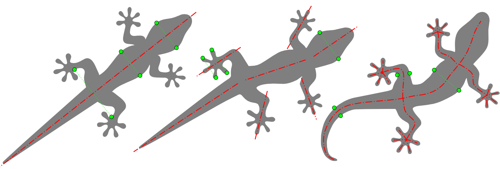
Figure 1: Three planar solid objects $\mathcal{O}_{a}$, $\mathcal{O}_{b}$, $\mathcal{O}_{c}$ and their respective axes of symmetry. The planar symmetry relations (dotted green lines) between a few pairs of points (green dots) have been highlighted.

In order to be able to generate a compact representations we can observe that most objects present a certain degree of redundancy in the information they convey. Indeed, in a geometric setting, this redundancy can be measured by the symmetry of the object. Intuitively, by removing the redundant information from an object that can be inferred through symmetry, we should be able to obtain more compact representations.

In an object, symmetry presents itself at different levels and by exploiting it we can create different levels of shape abstraction. For instance, consider the symmetries of the 2D solid object provided in Fig. 1. For simple shapes like $\mathcal{O}_{a}$, a single symmetry axis captures the global structure of the shape. However, such a global relationship is not always suitable. For example, by performing a simple quasi-rigid articulation of $\mathcal{O}_{a}$ we can obtain $\mathcal{O}_{b}$, where a global symmetry axis is now insufficient. To address this problem we could use multiple, more localized, axes of symmetry. However, when the shape undergoes even more complex types of articulation, like $\mathcal{O}_{c}$, even the use of a limited set of axes of symmetry becomes too restrictive. The solution to this problem can be found by considering symmetry at its finest level. Each pair of points in the shape is linked by a infinitesimal symmetry relationship and their centres of symmetry can be linked together to form a curvilinear axis commonly referred to as the skeleton of the shape.

Historically, the extraction of skeletal representations can be dated back to Blum’s work on the Medial Axis Transform [Blum 1967], which tracks the loci of maximally inscribed circles in two dimensional shapes. Although the MAT of a shape is unique, many alternative definitions exist, which I will discuss in

2 medial:definitions

. Each of these definitions highlight different properties (

3 medial:properties

), which in turn can be exploited for its computation (

4 medial:computation

). Of all these alternatives the most noteworthy in the context of this discussion is the one provided by [Blum 1973], which re-formulates the medial skeleton as the Symmetry Axis Transform of the shape: an attempt to identify infinitesimal (i.e. local) reflectional symmetries.

In two dimensions, we can use the infinitesimal reflectional symmetries encoded by the MAT to create curvilinear skeletons. This simple network of curves provide us with the desired concise shape representation. Unfortunately, when we extend our attention to the three dimensional objects it retains its curvilinear characteristics only when we restrict our consideration to networks of tubular structures. For more general shapes, the medial skeleton, while still computable, is composed of sheets (two dimensional manifolds) stitched together in a complex fashion [Giblin and Kimia 2004]. Even though medial representations of 3D objects are still useful in many applications (

5 medial:applications

), there are situations in which a simpler curvilinear representation is beneficial. These curvilinear representations of 3D shapes are commonly referred to as curve skeletons and will be the subject of

6 skeletons

.

Apart from medial skeletons, where unique and precise definitions (

7 medial:definitions

) are available, there are multiple ways to define curve skeletons and their computation (

8 skeletons

) is consequently application dependent. Typically we can think of the skeleton as a graph-like coding of the shape’s essential structure (

9 skeletons:properties

). This encoding attempts to represent shapes in ways that agree with human intuition: by representing connected components and the way they connect to form a whole. Thus, curve skeletons can be thought of as shape descriptors: a compact and expressive representation suitable for solving tasks which are computationally expensive if performed on large data sets.

10 Medial skeletons

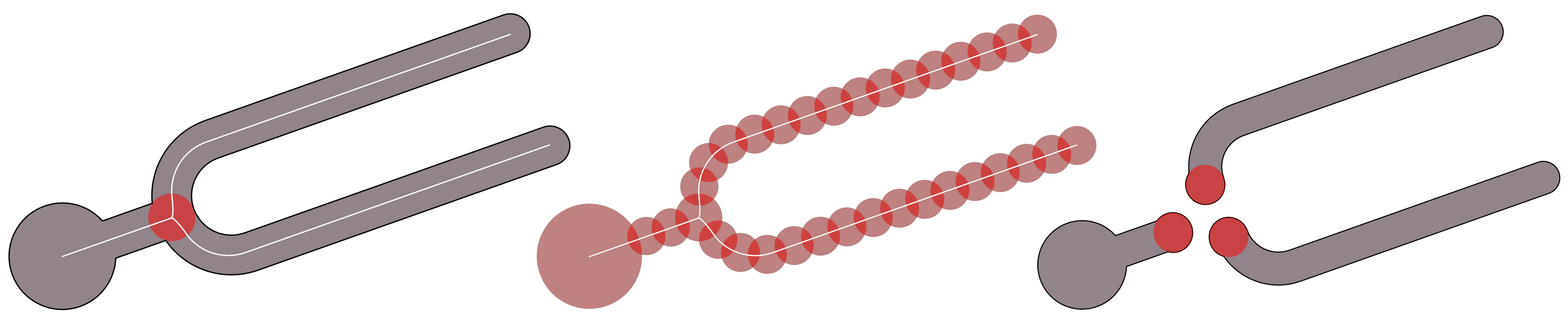
Figure 2: Medial Axis Transform essentials: (a) a planar solid object (gray), its medial axis (white) and one of its maximal inscribed balls (red); (b) the superposition of a subset of medial balls and its ability to capture the original geometry; (c) the branch structure of the medial axis can be used to decompose the shape in meaningful parts.

The concept of medial skeletons originated in the context of two dimensional shape understanding. It was created as a way of reducing the large amount of information carried by a shape down to a “skeleton” of crucial information that can be more readily assimilated. In Figure 2 an example of medial skeleton for a planar shape is shown. Note how the medial skeleton is able to effectively capture the parts that compose the shape and the way in which they are interconnected to form the whole.

Medial skeletons can be defined in many ways, as discussed in

11 medial:definitions

. As the medial skeleton of a shape is unique, these definitions are equivalent and reporting just one of them unequivocally defines medial skeletons. Nevertheless, these alternative formulations are very informative: they reveal essential shape properties which I will further discuss in

12 medial:properties

. These properties will offer key insights that will help provide the foundations for the creation of algorithms for skeleton extraction (

13 medial:computation

) and their practical application (

14 medial:applications

).

14.1 Defining medial skeletons

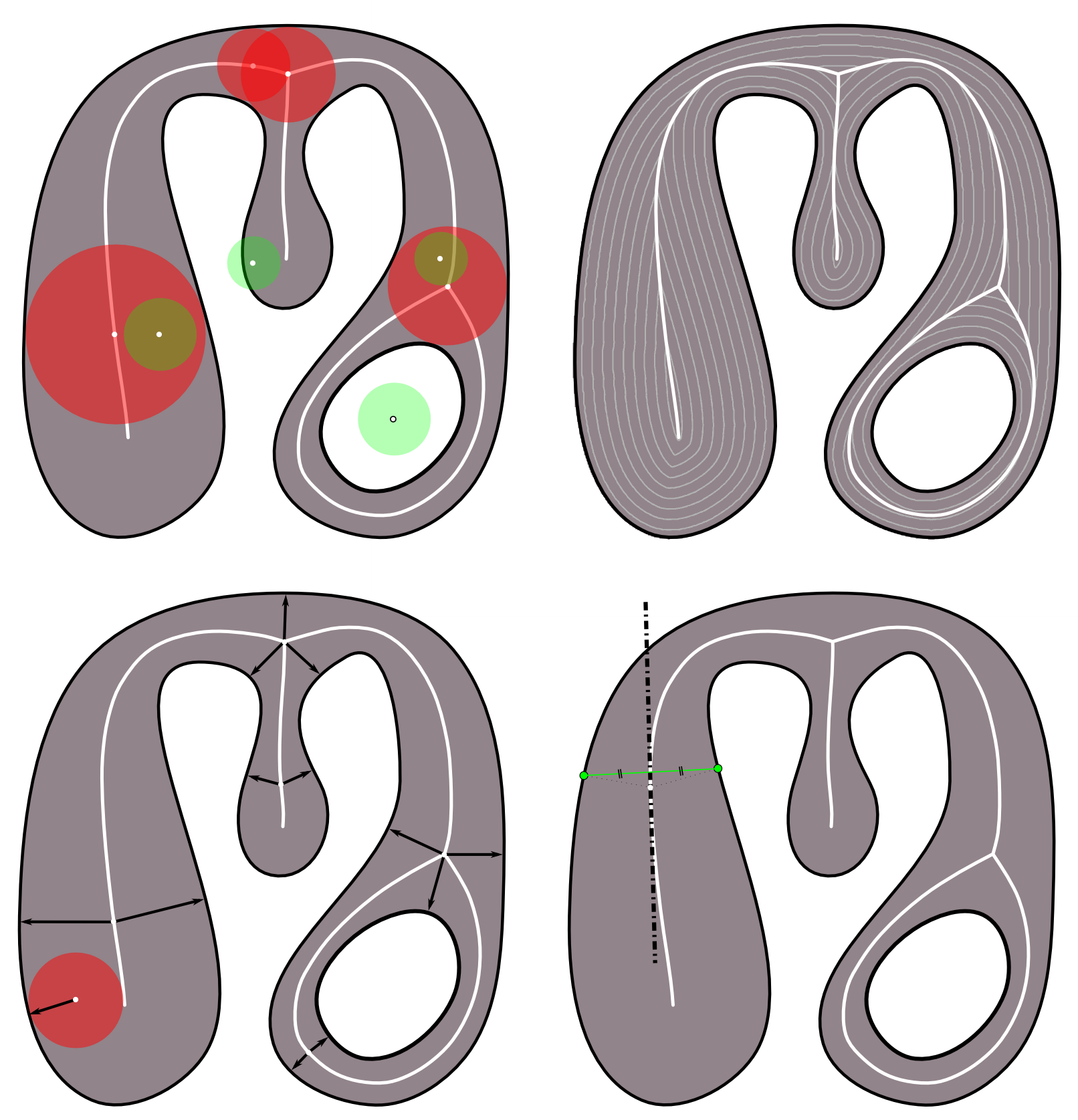
Figure 3: The four possible definitions of medial axis, in lexicographical order: (a) only the centres of maximally inscribed balls, colored in red, are part of the medial axis; (b) the medial axis as the shock graph of grass-fire evolution, the location of the boundary at different times is illustrated by thin white lines; (c) only points on the medial axis have more than one corresponding point on the shape boundary; (d) the medial axis links boundary points with an infinitesimal reflectional symmetry relationship.

In this section we will formally define medial skeletons of a shape. In this context a shape is nothing but a solid object $\mathcal{O}\subset\mathds{R}^{n}$ with boundary $\mathcal{S}=\partial\mathcal{O}$. Note that while I will define them and discuss their properties predominantly in two dimensions, these, unless otherwise noted, generalize to three dimensions. In $\mathds{R}^{2}$ we will refer to the $\mathcal{S}$ as the “contour” of the shape while in $\mathds{R}^{3}$ it will be simply referred to as the “surface” of the object. Also note that while in general the medial skeletons can be defined both for $\mathcal{O}$ and its complement space $\mathds{R}^{n}\setminus\mathcal{O}$, our focus will be on the skeletons of $\mathcal{O}$: the internal medial skeleton.

Maximally inscribed balls

The original idea of medial skeletons was introduced in the two dimensional domain by [Blum 1967]. Blum proposed that the skeleton of an object $\mathcal{O}$ can be extracted by fitting maximally inscribed balls^†in $\mathcal{O}$ and noting the locus of their centres (see Fig. 3-a). By augmenting the location of these centres $\mathcal{M}$ with the radius of the corresponding spheres $\mathcal{R}$ we obtain the Medial Axis Transform $\left[\mathcal{M},\mathcal{R}\right]=\textbf{MAT}(\mathcal{O})$.

Definition 14.1.

The Medial Axis Transform of $\mathcal{O}$ is the set of centres $\mathcal{M}$ and radii $\mathcal{R}$ of all the maximal inscribed balls in $\mathcal{O}$.

Note that since we only consider balls which are maximal, many inscribed balls and their associated loci will simply be discarded. The representation that we will obtain will consequently be sparse: the medial axis of $\mathcal{O}\subset\mathds{R}^{n}$ has at most dimensionality $n-1$. In addition, by superimposing medial balls of radius $\mathcal{R}$ at locations $\mathcal{M}$ we can recreate the original shape $\mathcal{O}$. This allows us to understand how the MAT is indeed a transform as it admits invertibility.

While Blum’s original definition provides us with much insight on its capabilities, it is hard to think in terms of maximally inscribed balls. For this reason a more commonly known definition is the one based on the grassfire analogy.

Grassfire analogy

Imagine $\mathcal{O}\subset\mathds{R}^{2}$ as if it were a patch of grass whose whole boundary $\mathcal{S}$ is set on fire at $t=0$. The fire will propagate isotropically from the boundary towards the interior of the shape with uniform speed along the normals $\mathbf{n}$. At certain locations, the fire fronts coming from different parts of the shape will meet and quench, thus defining a shock graph [Kimia et al. 1995]:

Definition 14.2.

The Medial Axis Transform of $\mathcal{O}$ with boundary $\mathcal{S}$ is given by the shock graph of the motion $\dot{S}=-\mathbf{n}$ and the time $t$ at which each shock is formed.

This definition not only stands at the core of many medial axis computation algorithms, which we will analyze in

15 medial:computation

, but it also allows us to intuitively understand why these skeletons are called medial. As two different sides of the boundary move at the same speed, their quenching location is located deep in the object, along its centreline.

Maxwell set

As the grassfire propagates isotropically, quench points will always be equidistant from the boundary. Consequently medial points are always associated with at least two (Euclidean) closest points on $\mathcal{S}$. This very property lies at the core of the Maxwell set definition of Medial Axis Transform [Mather 1983]:

Definition 15.1.

The Medial Axis Transform is the set of locations $\mathcal{M}$ internal to the object with more than one corresponding closest boundary point and their distance $\mathcal{R}$ from the boundary $\mathcal{S}$.

This definition has a key importance in the geometric setting. In

16 medial:computation:voronoi

we will discuss how this lies at the basis of medial extraction algorithms based on the Voronoi diagram.

Symmetry axis

Let us momentarily restrict our attention to objects with $C^{1}$ continuous boundaries. If we take a points $x\in\mathds{R}^{2}$, then the closest point on the boundary $s^{*}\in\mathcal{S}$ will define a ball $\mathcal{B}_{x,r}$ centred at $x$ of radius $r=\|x-s^{*}(x)\|$. This ball can be proved to be tangent to $S$ at $s^{*}$ [Amenta et al. 1998b]. If we restrict our attentions to medial points, which have at least two closest boundary points, then the associated medial balls will be bi-tangent to $S$:

Definition 16.1.

The Medial Axis Transform of $\mathcal{O}$ is the set of centres $\mathcal{M}$ and radii $\mathcal{R}$ of all the inscribed balls in $\mathcal{O}$ which are bi-tangent to its boundary $\mathcal{S}$.

Interestingly, the locus of bi-tangent balls was introduced by [Giblin and Brassett 1985] under the name of symmetry set. Consequently, the medial axis can be seen as a subset of the symmetry set, where only inscribed balls are to be considered. This simple observation underlines how skeletons can be thought of as a representation of symmetry axis as discussed in

17 intro

. Furthermore, note that while this equivalency required smooth boundaries, it extends to non-smooth ones by considering bi-tangency in the general sense.

17.1 Medial axis properties

The definitions from

18 medial:definitions

gave us much insight on what medial skeletons, or better, Medial Axis Transforms are. First, we understood why it’s medial, as it is located in the middle of the shape. Then we understood why it’s an axis, by observing its interpretation as an infinitesimal symmetry axis and its correlation to the symmetry set. But most importantly we understood it is a transform as it is unique and fully invertible. Consequently, the Medial Axis Transform can be thought of as a dual representation of shape, which exhibits particular properties of the shape. In this section we will focus on three core properties: 1) its ability to compactly represent topology, 2) the association between medial branch and shape part and 3) the ability to encode local shape volume.

In two dimensions, skeletons have received much attention as they are very effective at capturing the topological properties of the shape. Indeed, it can be shown how a shape and its medial axis are homotopy equivalent [Lieutier 2003]. Although both volumetric and boundary representations have this ability, the skeleton is able to represent topology more compactly by means of a lower dimensional construct. Remember that for a $\mathds{R}^{n}$ solid, the medial skeletons will have at most dimensionality $n-1$. Consequently, for two dimensional objects this will result in one-dimensional (curvilinear) medial skeletons. In a similar fashion, a three dimensional tubular shape can be represented by a medial skeleton as a collection of centrelines that split and join to encode the object topology. However, when we move our attention to 3D solids, medial skeletons will not be curvilinear, as they can contain up to $(3-1)$D construct: a collection of two-manifolds, curves and points in space (see Figure Skeletal Representations and Applications-b). For this reason the representation of topology in three dimensional data is more commonly performed by curve skeletons (see Figure Skeletal Representations and Applications-c) discussed in

19 skeletons

.

Medial branches and the “curse of instability”

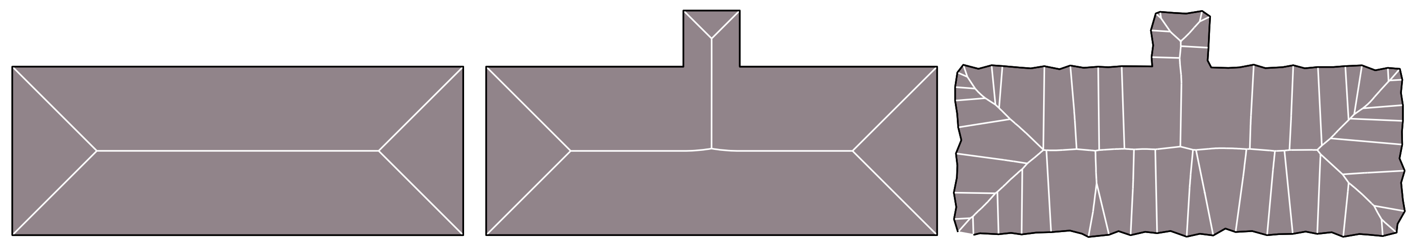
Figure 4: (a) Medial axis of a simple rectangular polygon. (b) Inserting a new feature creates localized changes in the skeletal structure. (c) The classical medial axis is unstable w.r.t. small scale features (i.e. noise)

.

By observing Figure 2 we can see how the medial skeleton does not exclusively capture the topology of the shape. Indeed, there would be no topological difference in between the tuning fork and any other planar shape homotopic to a disk. In fact, the medial is composed of a set of branches which are descriptive of the shape structure – it decomposes a shape in parts and they way in which they are interconnected (Figure 2-c). In order to better understand the limitations of medial skeletons, it is important to see what causes the creation of skeletal branches. To analyze this behaviour we can restrict our attention to planar polygons, whose medial axis transform simply consists of straight lines and parabolic arcs. In this simplified scenario, illustrated in Figure 4-a, we have a straightforward relationship: a medial branch can be found for every convex vertex of the boundary. This is indeed a cause of concern, since as illustrated in Figure 4-(b,c) polygonal objects with very similar geometry can result in very different medial skeletons. Ideally we would desire to have a branch for any “important” geometric part/feature of the shape. Here, the concept of importance is to be intended in terms of relative geometric scale w.r.t. other shape features. Note however that the classical medial skeleton is scale insensitive: the addition of an arbitrarily small geometric feature results in large, yet local, change on the medial axis. This property (or lack thereof) is known in the literature as the stability of the medial axis [Attali et al. 2009] and will be the subject of

20 medial:computation:stability

.

Correspondence and local thickness

By observing Figure 3-c we can perceive the existence of a very natural link between points on medial axis surfaces and points on the object boundary surfaces. Definition 15.1 allowed us to understand the first of these links: for each point on the medial axis there is one or more corresponding points on the boundary of the object. It is interesting to note that for at least $C^{1}$ smooth boundaries the opposite relation is quite different as for each point on the object boundary there is exactly one corresponding point on the medial surfaces. This observation is extremely important because it allows us to attach to each of the boundary points the size of the corresponding medial ball $\mathcal{B}$. The injectivity of the correspondence allows us to transport the scalar function $\mathcal{R}$ defined on $\mathcal{M}$ onto the shape surface $\mathcal{S}$. This scalar function defined on the surface is extremely important as it provides a formal way to define local shape thickness whose applications will be explored in

21 medial:applications

.

21.1 Medial axis computation

A large body of work exists on medial axis computation. In this section I will briefly describe the core idea behind these solutions. In geometry processing objects are most commonly represented by their boundary. For this reason I will introduce and describe methods that are progressively more suitable for these representations.

21.1.1 Exact medial computation

Regardless of the representation, if we are given an exact description of the shape then it should also be possible to compute an exact medial axis representation. Typically these exact computations follow the intuition behind the Maxwell set definition. For example if the boundary of an object is represented as polygons, then we can extract the medial axis by computing their bisectors as shown by [Lee 1982, Held 2001] in two dimensions and [Culver et al. 2004] in three dimensions. Note that the extraction of the exact medial axis is not restricted to piecewise linear representations. Recently the authors of [Tzoumas 2011] demonstrated how to compute the medial axis of rational curves in the plane, while [Musuvathy et al. 2011] addressed a similar problem in the three dimensional domain.

The extraction of exact medial representations, albeit possible, suffers from two major shortcomings. First of all, none of the methods above is able to deal with large datasets, like the ones typically found in most practical applications. This complexity is due to the fact that to compute the exact medial axis we have to solve systems of high degree algebraic equations. But even more importantly, in most scenarios geometric shapes are not known exactly. Shapes are indeed represented by different kinds of approximation, thus exactly extracting the medial axis is often unnecessary. For these reasons we will now move our attention to algorithms for approximate medial axis extraction and discuss the quality of this approximation.

21.1.2 Topological thinning

In the discussion of Definition 14.1 I highlighted the fact that the medial axis is a compact structure, with a much smaller volume than the original object, and how this structure is necessarily contained within its boundaries. If we represent our shape as a set of voxels sampling its interior, then a simple idea to compute medial axis is to progressively reduce the volume from the outside-in until a “thin” axial representation of unitary thickness is obtained. This criterion lies at the base of topological thinning methods like the one in [Palágyi and Kuba 1999].

An atomic reduction in volume can simply be achieved by removing a voxel from the set. This removal has to be done carefully so not to alter the overall topology of the solid. Therefore, algorithms in this class typically have to specify complex local measures of connectedness for both interior and exterior. Also, as we generally desire skeletons that are medial within the shape, this removal needs to be performed isotropically: by simultaneously removing voxels from the whole surface. However, in highly discrete settings, perfect isotropy is hard to achieve. Consequently, most algorithms suffer of the drawback that the structure of the resulting set depends on the voxel processing order, often resulting in skeletons which are non smooth. In addition, in regions whose thickness is expressed by an even number of pixels/voxels, the set of centres of maximal balls is two voxels wide. In these regions further thinning is possible but this often results in an even rougher axis.

For all these reasons, thinning methods are far from optimal for computing medial axis of detailed surface geometry as we would incur in two levels of approximation: in the surface to volume conversion as well as in the computation of the axis.

21.1.3 Distance fields

Rather than working directly on a discretized representation of the surface it is often convenient to represent the shape by means of an Euclidean implicit function: a real valued function that stores the Euclidean distance from the surface to any point in space. As illustrated in Fig. 3-b the iso-lines of the distance field correspond to positions of the boundary undergoing normal motion. Exploiting this observation, distance field methods attempt to estimate the medial axis by analyzing the local properties of the distance transform. Of particular interest are its ridges: the regions where its derivatives are multi-valued, which correspond with medial shock graphs.

Once the distance transform is computed, the extraction voxel along its ridges can be performed in a number of ways. In [di Baja and Thiel 1996] the authors first detect critical points in the distance field and then connect them to produce medial skeletons. Alternative methods identify medial voxels by thresholding some scalar function computed from the distance field. These function generally describe the likelihood of the voxel to be located on the ridge of the distance transform, like the average inward flux in [Siddiqi et al. 2002] or the object angle extension of [Shah 2005]. In many scenarios a simple thresholding is not enough as it would corrupt topology. For this reason, distance field methods are often coupled with the topology preserving thinning procedures discussed in

22 medial:computation:thinning

.

Even though implicit functions are most commonly stored on uniform discrete grids, they offer a much better shape approximation quality than simple voxelization, as typically the distance to the surface can be interpolated within each voxel. Furthermore, while the complexity for the computation of the Euclidean distance transform by fast-marching [Sethian 1996] is typically $O(n\log n)$, it is often acceptable to use other computationally cheaper types of distances. For example, in [di Baja and Thiel 1996] by using city-block distance, we are able to reduce the complexity of this pre-processing operation down to $O(n)$.

While the domain is represented more accurately, some of the limitations of thinning methods apply to distance transform methods as well. The medial axis is represented by a set of discrete voxels, and it is still possible to find regions of non-unitary thickness, making it a less than optimal choice for medial axis computation of surface representations.

22.0.1 Voronoi methods

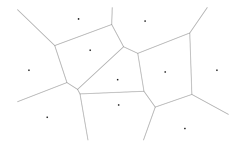
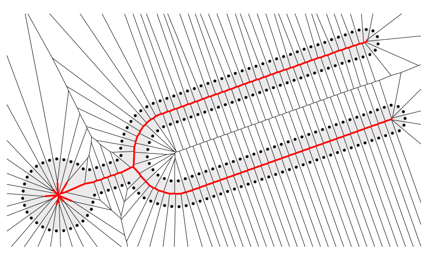
Figure 5: (a) The Voronoi diagram of six points in the plane. (b) The Voronoi diagram of points sampled from the boundary of a shape. Note how Voronoi vertices and edges fully contained in the shape boundary form an approximation of the medial axis.

The Maxwell set interpretation of the medial axis addressed in Definition 15.1 provides us with what we need to formulate the medial axis computation as a Voronoi diagram problem. This connection is immediately understood in two dimensions, as a Voronoi edge (vertex) is the locus of points that has two (three) closest neighbors. As the Voronoi diagram input is a point set, the boundary $\mathcal{S}$ of the object $\mathcal{O}$ typically needs to be sampled. Once a sampling is obtained, we can simply compute its Voronoi diagram $\mathcal{V}$. As illustrated in Figure 5, the medial axis can then be approximated by an appropriate subset of $\mathcal{V}$. In this section we will discuss the importance of the sampling and how to choose a proper subset to obtain good medial approximations.

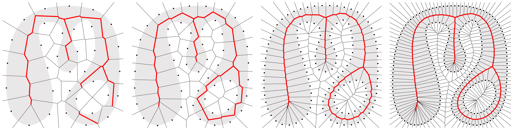
Figure 6: The Voronoi diagram of a sampled boundary with increasing uniform sampling density. The Voronoi vertices and edges completely enclosed within the boundary approximate the medial axis. As the density increases, the approximation quality improves. Notice how a minimum sampling distance is necessary to obtain skeletons that are topologically equivalent to the shape.

It was Blum in his original work [Blum 1967] that observed how, for a dense enough sampling of a smooth planar curve, the corresponding Voronoi diagram appeared to approximate $\mathcal{M}$. As illustrated in Figure 6, the denser the sampling of the curve, the better the medial approximation achievable. However, it was not until much later that [Brandt and Algazi 1992] proved that, given a dense enough uniform $\delta$-sampling^†, the subset of Voronoi fully contained within $\mathcal{S}$ correctly approximates the medial axis with a convergence guarantee. This result was then extended by [Attali and Montanvert 1997] where the requirement of an oracle knowledge of $\mathcal{S}$ was removed, and a proven topologically correct medial approximation was shown possible from a sampling of the surface only. Further extension was provided by [Amenta et al. 1998a], which suggested how uniformly sampling the boundary is often unnecessary and an adaptive $\epsilon$-sampling^†can be used.

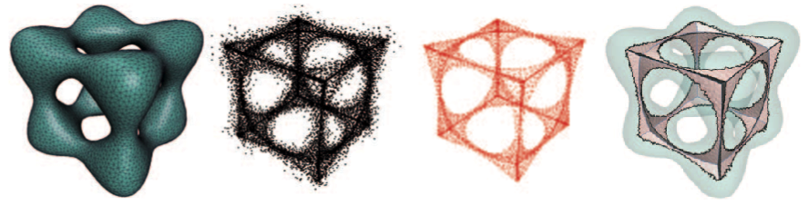
Figure 7: (a) A solid object in $R^{3}$ represented as a triangulation of its surface. (b) The internal subset of Voronoi vertices. (c) The internal subset of Voronoi poles. (d) Given a uniform surface sampling, the $\lambda$-medial axis, a subset of the Voronoi facets, approximate the medial surfaces.

Unfortunately, when we expand our interest to three dimensional objects, the results of [Attali and Montanvert 1997] or [Amenta et al. 1998a] do not directly hold. The problem is that, even for arbitrarily fine samplings, the Delaunay triangulation dual to the Voronoi diagram often presents sliver tetrahedra. These sliver tetrahedra correspond to Voronoi vertices, which neither fall in proximity of the medial axis nor are related to any prominent feature of the surface. To address this issue, [Amenta and Bern 1998] approximated the medial axis by a more restrictive subset of the Voronoi diagram: by only considering the Voronoi poles^†. The validity of Voronoi poles for medial approximation was formally verified by [Amenta et al. 2000], where the authors showed that for an $\epsilon$-sampled $C^{1}$ manifold, the poles approach the medial axis of the shape as $\epsilon$ vanishes. The validity of Voronoi poles is intuitively illustrated in Figure 7 where we visually compare their approximation power to the one of internal Voronoi vertices.

22.0.2 Stable medial axis

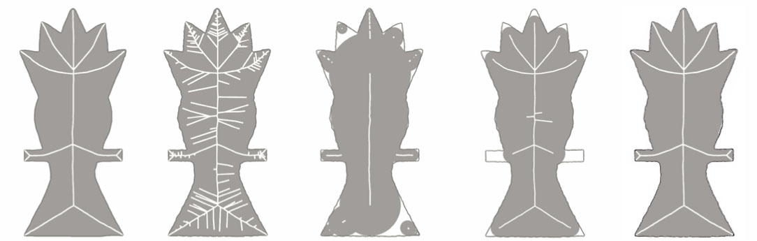
Figure 8: (a) A solid planar object and its medial axis. (b) Noise is added to the object boundary resulting in many spurious branches of the medial axis. (c) Filtering medial loci by object angle ($\lambda$-medial axis [Chazal and Lieutier 2005b]) captures features across different scales but results in large topological changes. (d) Filtering medial loci by the distance of the corresponding surface points ($\gamma$-medial axis [Amenta et al. 2001]) retains topology but removes small scale features before getting rid of all the spurious branches. (e) The global approach of the scale axis transform is able to remove the noise while retaining small scale features.

When using medial representations for shape processing, we would like for similar shapes to have similar medial representations. However, while the Medial Axis Transform provides a perfectly invertible (i.e. dual) representation, a major shortcoming is that, as discussed in

23 medial:properties

, it is not stable with regards to small geometric variations. This issue is particularly important when we consider samples that are noisy, as even slight amounts of noise can produce long spurious branches in the MAT. This noise can be caused by a measurement process, when samples have been acquired by scanning the surface of real a world object, or by the fact that we are sampling a discretization of the shape. Here, I will review a few selected alternatives for noise management while referring the reader to [Attali et al. 2009] for a more extensive coverage of the topic.

Typically, a simpler medial axis can be obtained by performing a smoothing operation, however, controlling the right amount of smoothing has been shown to be a very challenging problem [Attali et al. 2009]. For this reason, a large majority of the literature addresses the problem by considering the stability of a medial point either in terms of its local or global properties.

Local filtering criteria

One common way of creating medial skeletons is by pruning its branches according to some local criteria. A traditional choice lies in using some local measurement of a medial sample like the corresponding pair of points on the surface of Figure 3-c. For example, [Chazal and Lieutier 2004, Chazal and Lieutier 2005b, Chaussard et al. 2009] proposed the $\lambda$-medial axis, where medial samples whose corresponding surface samples have a circumradius larger than $\lambda$ are discarded. For particular choices of the $\lambda$ parameter [Chazal and Lieutier 2005a], the medial axis approximation is homotopic to the shape, and its approximation quality is provably convergent. Unfortunately, as it is illustrated in Fig. 8-b, this criterion doesn’t allow the capture of details across different scales, as important features of the shape are removed before eliminating all of the noise. An alternative choice was presented by [Attali and Montanvert 1996, Amenta et al. 2001, Dey and Zhao 2004, Sud et al. 2005], where the authors use the spoke aperture angle as a filtering criterion. However, while this approach is able to retain features at different scales, it might result in an axis whose topology is drastically different as we change the thresholding parameter as it is illustrated in Figure 8-c. The common problem is that since these solutions are highly local it allows them to be efficient and simple to analyze but unable to capture the multi-scale structure of the shape.

Global filtering criterions

Following a more global approach, we can compute the multi-scale importance of a medial branch based on volumetric approximations of the shape like in [Tam and Heidrich 2003] or by analyzing its global connectivity to maintain topological equivalence to the shape [Sud et al. 2005]. Alternatively, we can address the problem in a statistical sense by analyzing the resilience of a medial branch in a collection of shapes like in the works of [Styner et al. 2003] and [Ward and Hamarneh 2009]. However, because of its simplicity, the most interesting global solution to the problem is the Scale Axis Transform proposed in 2D by [Giesen et al. 2009] and successfully applied to 3D data by [Miklos et al. 2010]. In the scale axis, the global relationship between parts is obtained by scaling the medial balls of the shape by a factor $\delta$. Small medial balls, associated with small surface features and noisy medial branches, undergo a growth that is smaller than nearby large medial balls (i.e. larger nearby features). Following Definition 14.1, whenever one of these scaled balls is not maximally inscribed, it is removed from the set. A stable medial axis is then computed as the exact medial axis of the remaining set of de-scaled balls. As illustrated in Figure 8-e, the quality of the resulting medial axis is far superior to the one of more local methods.

23.0.1 Approximate medial measures

While the methods discussed up to this point provably produce convergent approximations of the medial axis, there are situations in which it is possible to compute coarser estimates. For example, in situations in which only a rough approximation of the medial surfaces is desired, the shape surface triangulation can be recycled like in the manifold medial approximation introduced by [Hisada et al. 2002]. Alternatively, in situations in which only an estimate of local thickness is required, the relatively expensive medial computation can be replaced by an (embarrassingly parallel) ray casting procedure [Shapira et al. 2008]. The distance field methods of

24 medial:computation:dfields

can exploit coarse-to-fine spatial discretizations, where efficient yet not-as-rigorous algorithms for thresholding can be used [Bloomenthal and Lim 1999]. Differently from

25 medial:computation:stability

, the generation of stable representations can be aided by the use of templates offering pre-determined connectivity [Pizer et al. 2003] or by softening some of the strict requirements imposed by the medial axis transform [Pizer et al. 2011].

25.1 Medial axis applications

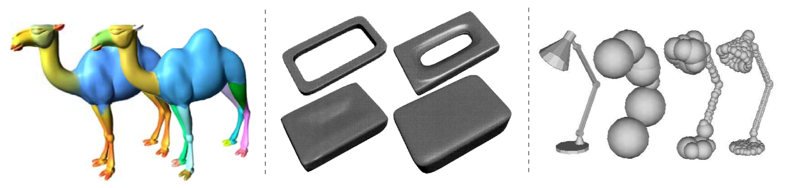
Figure 9: (a) The approximation (left) of the local radius in [Shapira et al. 2008] and its application to segmentation (right). (b) Two shapes (on the main diagonal) are blended into each other by exploiting the volumetric structure of the medial axis in [Blanding et al. 2000]. (c) An object represented as a triangulated surface is decomposed by [Hubbard 1996] in a set of spheres to accelerate collision detection.

The properties of the medial representation do not only lay the foundations for its computation but also give us the fundamental intuition to understand the many applications it has in practical scenarios.

The volumetric capabilities of the MAT has been exploited in a number of ways. In the medical domain, it has been used as a way of measuring local volumetric properties of the shape [Näf et al. 1997], as well as for segmentation by fitting volumetric templates and statistical analysis [Pizer et al. 2003]. Alternatively, in 3D the local volume can be clustered to segment the shape in patches of similar thickness as shown by [Shapira et al. 2008], used as a prior for hole filling [Tagliasacchi et al. 2011] or to facilitate shape modeling of organic shapes [Angelidis and Cani 2002]. The medial positioning of its curves can be exploited as an alternative to implicit functions to compute shape blends [Blanding et al. 2000], as well as for navigation purposes [Paik et al. 1998], while their interpretation as a set of inscribed spheres can be used to generate a simplified model for collision detection [Hubbard 1996]. In 3D, the boundaries of medial surfaces have been shown to be associated with important perceptual features [Hisada et al. 2002], which can be exploited to reduce the complexity of registration tasks [Chang et al. 2004]. As suggested by [Storti et al. 1997], the generation of stable medial axis can be exploited in the generation of shape simplification schemes from a volumetric point of view like in [Tam and Heidrich 2003], while the continuous connection existing between medial surfaces and shape surface [Shaham et al. 2004] describes the volume in a way that can be exploited for the generation of hexahedral meshes [Tchon et al. 2003].

Perhaps the most important characteristic of the medial axis is that, in two dimensions, it is able to reduce the shape to a network of 1D curves. For 2D shapes, this graph-like representation lies at the core of a large set of algorithms that address the important problems of shape retrieval and correspondence [Siddiqi et al. 1999]. Unfortunately, these techniques do not directly apply to 3D shape because, as discussed in

26 medial:properties

, their medial axis in the general setting is not composed of 1D curves. Thus, to be able to apply these methods with minimal modifications, we need to be able to generate curvilinear representations for 3D shapes. These curvilinear representations are called curve skeletons and their computation and applications will be the subject of

27 skeletons

.

We will conclude this section by describing two core applications of medial axis. These applications are possible thanks to the fact that the MAT offers a fully equivalent (i.e. dual) representation of the surface of an object.

27.0.1 Surface reconstruction

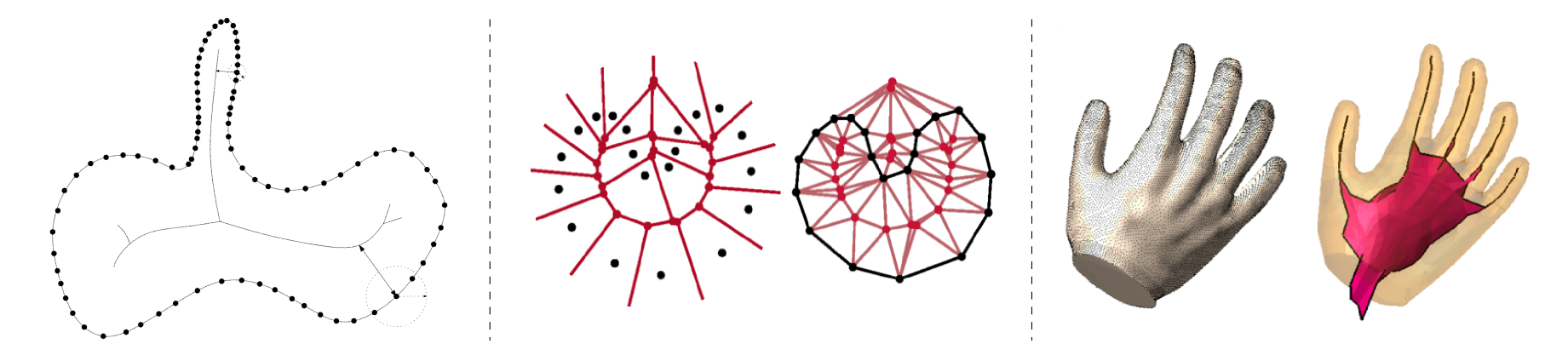
Figure 10: (a) An example of the multi-scale $\epsilon$-sampling; note how higher sampling density is required in thin regions, measured by the local feature size. (b) The medial axis is used to discard Delaunay edges connecting opposite sides of the shape’s boundary in [Amenta and Bern 1998]. (c) An acquired point cloud (left) is reconstructed into a surface and its medial axis (right) by [Amenta et al. 2001].

Given a sampling of the surface of a solid object, the problem addressed by surface reconstruction is the one of obtaining a parametrized (e.g. triangulated) representation of the surface.

In this context the medial axis was shown by [Amenta and Bern 1998] to be essential in formalizing the minimal requirements of sample density. Intuitively, we would like a larger sampling density in regions of high curvature, so as to be able to capture minute surface variations. At the same time, an increased number of samples is needed in narrow regions to properly capture the shape’s topology. To address both these requirements, [Amenta and Bern 1998] introduced the $\epsilon$-sampling, where the necessary local sample density depends on the local feature size: the distance to the closest point on the medial axis.

The contributions of medial representations do not end here. In particular, a way to approach the reconstruction problem is by computing the Delaunay triangulation and discarding a subset of its elements [Edelsbrunner and Mücke 1994]. In [Amenta et al. 1998b], the authors extended this approach in an intuitive and powerful way: given an appropriate $\epsilon$-sample, they show that, by discarding elements whose circumsphere contains a portion of the medial axis, results in a topologically correct reconstruction of $\mathcal{O}$. This method and its essential relationship with the medial axis created the basis for much work in the field of combinatorial reconstruction [Cazals and Giesen 2006].

27.0.2 Shape manipulation

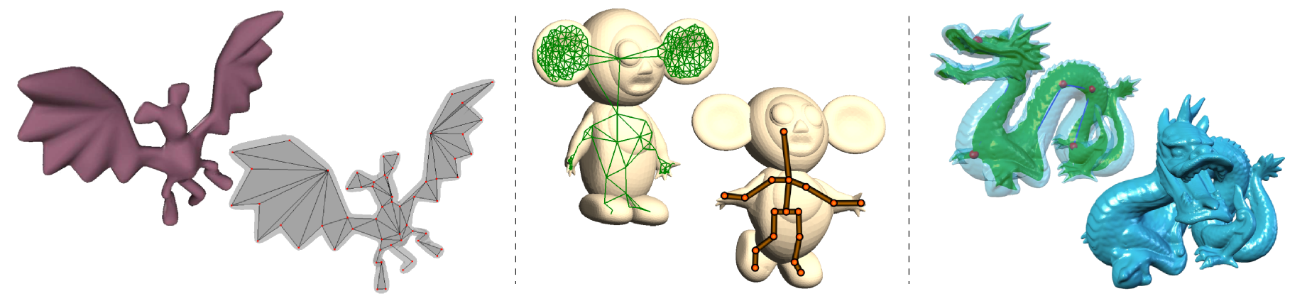
Figure 11: (a) An example of a model produced by the medial axis based framework of [Angelidis and Cani 2002]. (b) A graph approximating the medial axis is used as an embedding domain for a template skeleton, allowing to re-use animation rigs and produce new poses [Baran and Popović 2007]. (c) An example of a deformation achieved by the volume preserving framework of [Yoshizawa et al. 2007].

Developing geometry-manipulation tools for end users is a core problem in geometry processing. The medial axis offers an alternative to the more commonly used surface based methods by exploiting the volumetric information of the shape captured in the axis.

In [Storti et al. 1997] the authors propose to use the medial domain as an alternative to surfaces for shape parameterization, thus creating the foundations for the widely used m-reps of [Pizer et al. 2000] and the shape modeling frameworks of [Angelidis and Cani 2002]. Intuitively, by sparsely sampling the medial axis, the shape can be manipulated by modifying the position and radius of medial loci and then reconstructing/deforming the object surface.

Following a similar paradigm, [Bloomenthal and Lim 1999] investigated a way of connecting the use of geometric (medial) skeletons to traditional kinematic skeletons for shape animation. Rather than directly expressing surface vertex positions as a function of the kinematic skeleton, the author proposes to first animate the medial skeleton and then reconstruct the surface from its medial representation. Further connections between these two structures were also investigated by [Baran and Popović 2007], where instead of attempting to model surface animation by means of medial axis, the authors consider the medial domain an appropriate space for fitting a template of a kinematic skeleton. Traditionally, the transformation of animated surface vertices is obtained by a linear combination of transformations defined on kinematic skeletons. While these weights are typically set by artists by a time consuming trial and error process, [Bloomenthal 2002] uses the medial axis and the radius function defined thereon to create a convolution scheme that is able to completely automatically create blending weights, resulting in natural-looking surface animations.

Rather than directly modifying the medial axis, or use a kinematic skeleton as a control structure, in [Yoshizawa et al. 2003, Yoshizawa et al. 2007], the authors investigated the use of freeform deformation of the medial surfaces for shape deformation. Their solution presents two strong advantages: first of all, thanks to the volumetric nature of medial representation, more natural large scale deformations can be achieved as local thickness is preserved; furthermore, self-intersections, which often arise when large deformations take place, can efficiently be corrected by exploiting the volumetric nature of medial representations.

28 Curve Skeletons

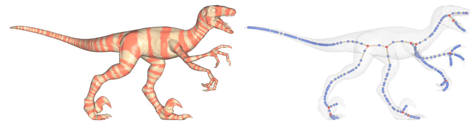
Figure 12: (a) A three dimensional object; the colour coding expresses the correspondence between portions of the surface and vertices on the curve skeleton. (b) An example of a curve skeletal representation extracted by [Au et al. 2008].

Curve skeletons were introduced as a way of providing a curvilinear (a one dimensional construct) representation of three dimensional shapes. As I have thoroughly discussed in previous sections, this necessity came from the fact that classical medial axis generally produces two-manifold elements when applied to three dimensional shapes. It is important to note that while medial skeletons are precisely and uniquely defined, the same doesn’t apply to curve skeletons. There is no universally accepted rigorous definition of what a curve skeleton is. A notable exception is the medial geodesic skeleton recently defined by [Dey and Sun 2006]. However, since it is computed as a subset of the medial axis, it also inherits all of its stability issues and has consequently received little attention in applicative scenarios. Without restricting ourselves to this formal definition, we can compute curve skeletons in multiple ways; these different methods will be the subject of

29 skeletons:computation

. The lack of a common formal background makes the task of comparing these different algorithms quite difficult. An attempt to compare these techniques was performed by [Cornea et al. 2007], where the authors defined a set of desired curve skeleton properties and then discussed several algorithms accordingly. In

30 skeletons:properties

we will briefly discuss these properties, which will find a direct use in creation of curve skeleton extraction (

31 skeletons:computation

) and their applications (

32 skeletons:applications

). Note that, similarly to

33 medial

, I will focus my attention to methods which are suitable for surface-based object representation of 3D geometry.

33.1 Properties

The only strictly necessary property that a curve skeleton should have is that it needs to be thin – a one-dimensional entity embedded in the three dimensional domain. As in medial skeletons, it is also often required that this network of curves is homotopic to the shape – that they retain the ability to accurately encode the topological structure of the object they represent. It is also important that curve-skeletons offer part-awareness: its branches should provide a one-to-one association with “important” geometric features on the shape. As the graph connecting branches establishes a relationship network, by computing skeletons at different resolutions we obtain a way to represent shape in a hierarchical fashion. Additionally, we would like their computation to be robust, in the sense that the presence of surface noise should not result in the generation of spurious branches. The smoothness of curve skeletons is also important, not only for its visual appeal, but also because it improves compactness, as smooth structures are generally representable with a smaller set of geometric elements.

Furthermore, as curve skeletons are often employed as representations of solid objects, it is often desirable for its curves to be contained within the object. In some scenarios, an ever more restrictive requirement on its positioning is necessary: the curves are required to be centred within the object, in a similar way in which MAT skeletons are medial within the shape. The positioning of the medial axis is also critical in situations that require reliability: where we ask that every point on the surface is visible from at least one curve skeleton location. It is important to note that, from a geometrical point of view, curve skeletons do not truly provide an alternative shape representation, as we cannot perfectly reconstruct the original shape given a curve skeleton. Curve skeletons are instead to be interpreted as shape descriptors: a compact way of capturing essential geometrical and topological information. In order to be able to transfer information from the surface to the curve skeleton it is necessary that proper correspondences exist between points on the surface and points on the skeleton. For example, these are essential for the generation of an approximated reconstruction of the object. This can be achieved by superimposing a set of simple primitives (e.g. spheres, ellipsoids or by sweeping planar curves) along the curve skeleton. The parameters of these primitives can be inferred by analyzing the corresponding surface geometry.

It is important to note that not all properties are essential in every application scenario. Furthermore, strictly requiring a skeleton to offer one of these properties might make the satisfaction of others unfeasible. As an example, it is hard to obtain centred (in a medial sense) yet robust skeletons, because the medial axis is sensitive to small surface perturbations. Similarly, we could achieve better reconstruction by introducing extra branches in the representation, albeit at the cost of losing part-awareness.

33.2 Curve skeleton computation or “skeletonization”

In the literature, curve skeletons are computed or “extracted” following few alternative philosophies. Some algorithms, discussed in

34 skeletons:computation:medial

, focus on reducing the medial skeleton surfaces down to one dimensional structures. In

35 skeletons:computation:potential

I will discuss those that attempt to modify the notion of distance in order to create curves, as opposed to surfaces, which lie medially within the shape. In

36 skeletons:computation:topological

I will move my focus to solutions based on topological analysis, where the core aim is to generate homotopy preserving skeletal representations. Other very successful methods, described in

37 skeletons:computation:zerovolume

, focus on the fact that we are indeed looking for a curve. I will conclude with

38 skeletons:computation:grouping

, where I will describe very-application oriented techniques, that construct curve skeletons by grouping surface elements according to particular properties, and then define the skeleton as the graph describing how these components are glued together to form the whole.

38.0.1 Skeletonization by medial axis processing

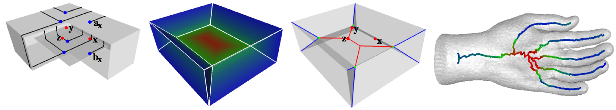
Figure 13: An illustration of the fundamentals of the described in [Dey and Sun 2006]. (a) Three points (red) on the medial axis of a cuboid; their corresponding surface points (blue), and the shortest paths on the surface between these points (black). (b) The medial geodesic function on the medial axis of shape. (c) High divergence points of the medial geodesic function define the curve skeleton. Note how only $y$ and $z$ are on the skeleton as they are associated with more than one shortest path. (d) The curve skeleton of a noisy hand model is also noisy as it is defined as a subset of the medial axis.

The medial axis of a solid object conveys much of the essential structure of the shape. However, the medial skeleton is geometrically complex as it is composed of a set of surfaces. A simple approach to compute a curvilinear representation of the shape is to prune the medial axis surfaces down to a linear structure. Many heuristics can be used to prune the medial sheets to a line-form; for example, the authors of [Lee et al. 1994] use a thinning method similar to the one described in

39 medial:computation:thinning

. A very interesting solution along these lines is the one proposed by [Dey and Sun 2006], where the authors proposed to extract the skeleton as the shock graph of the Medial Geodesic Function, a scalar function defined on the medial axis surfaces. Given a point $m\in\mathcal{M}$ and its two corresponding surface points $s_{1},s_{2}$, this function is defined as $\text{MGF}(m)=d_{\mathcal{S}}(s_{1},s_{2})$, where $d_{\mathcal{S}}(s_{1},s_{2})$ is the geodesic distance on $\mathcal{S}$ between the two points. The theoretical argument on the existence of this shock graph provided by [Dey and Sun 2006] make medial geodesic skeletons the only mathematically precise version of curve skeletons. Nevertheless, curve skeletons extracted in this fashion suffer severe limitations. Its computational complexity is large, as it necessitates geodesic distances between every pair of surface vertices. Furthermore, the sensitivity of medial axis to surface noise, discussed in

40 medial:properties

, result in the extraction of noisy skeletons like the illustrated in Figure 13-d.

40.0.1 Skeletonization by generalized field analysis

There exist alternatives to processes that erode the medial axis in order to generate curve skeletons that are well-centred within the shape. These are based on more complex (in particular less localized) ways of measuring the distance from the boundary [Hassouna and Farag 2008]. The value of the field at a position in space is computed as the average of potential fields of many boundary samples, and the skeleton extraction is performed by tracing curves seeded at critical points along directions of high divergence. Because of the inherent averaging, these skeletons are not only medial but often very smooth. A major problem with these methods is that they are not particularly suitable for surface based geometry: the field needs to be represented on a discretized volume and, most importantly, they tend to suffer from numerical instabilities. For these reasons they will not be further discussed and I simply refer the reader to [Cornea et al. 2007, Hassouna and Farag 2008] for more details.

40.0.2 Skeletonization by topological analysis

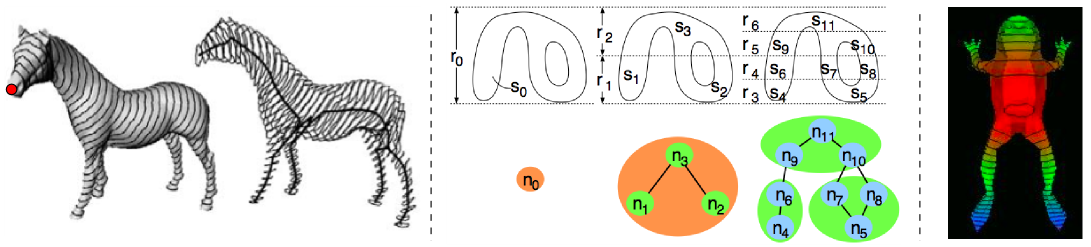
Figure 14: (a) A geodesic distance field sourced at the marked point is created onto the surface and its iso-contours are shown. The barycenter of surface portions between two successive iso-contours is used to build a curve skeleton like embedding of the topological graph [Lazarus and Verroust 1997]. (b) The $y$ coordinate is used as the field for topological analysis. By recursively refining its iso-contours, a multi-resolution topological graph is created [Hilaga et al. 2001]. (c) The iso-contours of the average geodesic function from [Hilaga et al. 2001] naturally capture the extremities of the articulated shape of a frog.

There are situations in which the core information about an object can be captured by the topological structure of its skeleton (i.e. loops and joints) rather than by its geometric attributes (i.e. curve locations and local radius). In Morse theory [Shinagawa et al. 1991], a real $C^{1}$ function $f$ defined on the surface $\mathcal{S}$ of a shape is able to capture its essential topological information: the critical points of $f$ encode the topological changes in the shape. More intuitively, the topological information can be extracted by looking at the iso-contours of $f$ and their distribution on $\mathcal{S}$ [Biasotti et al. 2000b, Natali et al. 2011] as illustrated in Figure 14.

In certain situations, like Figure 14-b the simple $y$ coordinate of boundary points is sufficient. However, there are many ways of creating $f$ and this choice is made according to the type of information we want to extract from the shape. While for a broad comparative analysis we refer the reader to [Biasotti et al. 2003], for skeleton extraction, a simple solution was introduced by [Lazarus and Verroust 1999]. Their idea is illustrated in Fig. 14-a, where $f$ is computed as the geodesic distance (or one of its approximations) from a selected source point $p$. Even though the seed point can be selected by heuristics, it is important to note that a single seed generally results in the selection of a preferred slicing direction. An example of the consequences of this choice is illustrated in Fig. 14-a, where we can easily discern a loss of structural detail in the skeleton. To solve these issues, [Mortara et al. 2003] proposed the use of a set of seed points on protrusions, which can be identified by searching for locations of high large gaussian curvature, while other methods like [Hilaga et al. 2001] compute the integral of the geodesic distance to all other surface points (See Figure 14-b,c).The limitation of all these methods is the necessity to pick an heuristic, as, according to the choice made, unforeseen topological loops can appear in locations where the wavefronts collide.

It is important to note that this class of algorithms typically offers limited geometric interpretation. The spatial location of a skeletal vertex (i.e. its embedding) is generally computed a posteriori – as the centroid of its corresponding surface points. Consequently, these methods generally offer lower quality geometric skeletons, and are more focused toward providing a correct topological representation. It is very important to note that in applications where topology is the core shape feature, very simple (and efficient to compute) choices for $f$ can be made, like the $y$ coordinate of Figure 14-b, and these are ensured to produce homotopy preserving curve-skeletons.

40.0.3 Skeletonization by contraction

The fundamental requirement of curve skeletons to be a line-like representation can be used for their computation. A line representation can indeed be thought of as a zero-volume solid. Thus, in order to be able to extract a skeleton, we can let the shape evolve in such a way that, at each iteration, its total volume is strictly decreased. In order to avoid loss of detail, this volume reduction, commonly referred to as contraction, needs to be performed in a controlled fashion. The method used to control contraction is the fundamental ingredient of the algorithms described in this section.

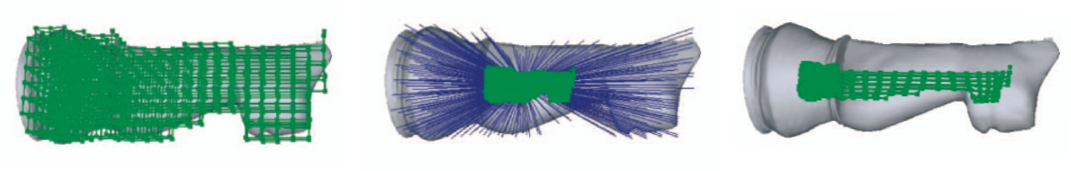
Figure 15: An illustration of the volumetric contraction proposed by [Wang and Lee 2008]. (a) The surface is first converted into a volumetric representation. (b) The edges of the volume are isotropically contracted, but by using the surface attraction constraints (blue) we can avoid the shape from collapsing to a point. (c) By using these attractors the collapsed volume retains the shape features.

Volumetric contraction

In [Wang and Lee 2008], the authors compute the curve skeleton of a volumetric model by applying a contraction procedure. If we think of the shape’s volume as a set of voxel centres connected by edges, it is intuitive to think that we could reduce the shape’s volume by uniformly scaling down the edge’s lengths. Clearly this isotropic scaling would quickly and meaninglessly shrink the shape down to a zero-volume point as illustrated in Figure 15-b. In order to prevent this from happening, the authors solve a constrained problem where the locations of voxels originally positioned nearby the surface are required not to move too far from their initial location. A fundamental problem in applying this technique to surface models is that it requires a volumetric contraction. Nevertheless the contribution of [Wang and Lee 2008] is important as it built the groundwork for the very successful surface based contraction method.

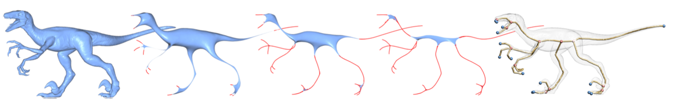
Figure 16: An illustration of the surface contraction proposed by [Au et al. 2008]. (a,b,c,d) From left to right the shape is contracted by applying curvature flow until the volume vanishes. To prevent over-contraction surface attraction constraints similar to [Wang and Lee 2008] are applied. (e) The contracted surface retains the original manifold topology and is collapsed to linear graph [Li et al. 2001].

Surface contraction

In [Au et al. 2008] the authors address the problem of volumetric contraction directly on a meshed surface representation. In the proposed solution they iteratively reduce the volume of the shape (i.e. contraction) by solving a constrained mean curvature flow (MCF). Motion by mean curvature is known to result in a volume loss at each iterations [Ruuth and Wetton 2003]. While performing MCF on the surface doesn’t cause a contraction as isotropic as [Wang and Lee 2008], surface attraction constrains need to be inserted in the system to make sure that branches do not undergo excessive shrinkage, thus, resulting in the loss of important surface features. The foundations for the success of this technique is that both the volume contraction motion and the feature preserving constraints can efficiently be encoded by a system of linear equations for which efficient solvers are available. Furthermore, as far as a proper Laplacian operator is used, the contraction procedure is not only insensitive to badly discretized surfaces (e.g. low quality triangulation), but since MCF is essentially a smoothing operation, it is also extremely robust to noise.

Topological contraction

While the methods above tackle the problem of contraction in a geometrical sense, it is interesting to know that it’s possible to reduce the overall shape volume by only using topological operations. In [Li et al. 2001], the authors propose to use iterative edge collapse to reduce a meshed surface to a set of simple segments, which have no incident faces (i.e. wingless). As the resulting set is a simple network of edges, this structure is ensured to be one dimensional. Furthermore, by choosing to collapse the shortest edge first (resulting in an overall $O(n\log n)$ complexity), the authors experimentally demonstrate how this solution results in approximatively-centred skeletons. While no strong theoretical foundations exist for topological contraction, this algorithm lies at the core of many skeletonization algorithms, as it is often employed as a post-processing step: to reduce a quasi-thin structure to a set of truly one dimensional primitives [Wang and Lee 2008, Au et al. 2008]. It is important to note that in situations in which the quasi-thin structure is already centred within the shape, the topological contraction does not alter the embedding, thus, preserving centeredness.

40.0.4 Skeletonization by property grouping

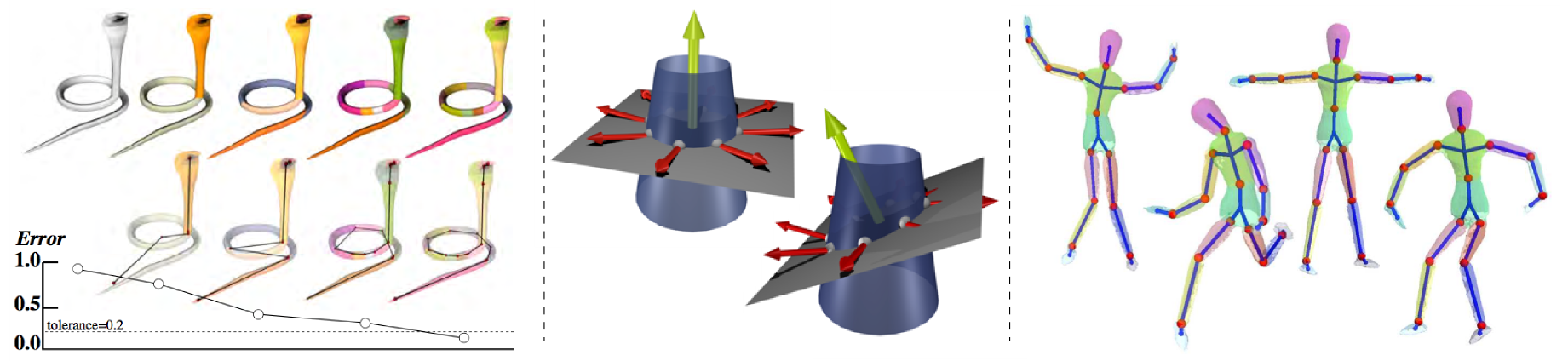
Figure 17: (a) A convex decomposition allows to recycle PCA axes as skeletal branches [Lien et al. 2006]; the finer the decomposition, the more accurate the skeletonization. (b) Local rotational symmetry of a group of samples can be measured by observing the arrangement of the surface normals on the gaussian image [Tagliasacchi et al. 2011]. (c) The articulation of a shape is essentially described by a set of locally rigid transformations [Anguelov et al. 2004]; these transformations can be identified and exploited to create a kinematic skeleton.

If we are given the curve skeleton of a shape, we are provided with a way of decomposing it in fundamental parts and their interconnections. Note that this relation can be considered in the other direction as well. If our application domain allows us to precisely identify what constitutes a part, then we can construct curve skeletons as the network of curves describing their spatial configuration. There are many ways to define appropriate grouping criteria for skeleton generation and, in this section, I will describe a few important examples.

Rotational symmetry

In

41 intro

I discussed how one way of interpreting a skeletal axis is by considering it as an axis of symmetry. For two dimensional shapes, it was reflectional symmetry that allowed us to define medial skeletons – by grouping pairs of locally symmetric points [Zhu 1999]. In three dimensions a different symmetry relationship can be exploited: rotational symmetry. Nevertheless, like in

42 intro

, the extraction of global rotational symmetry [Sun and Sherrah 1997] would only allow us to define a single global axis. Consequently, the generation of curvilinear representations can be achieved by considering symmetry at a local scale [Li et al. 2001]. The identification of local rotational symmetry (see Figure 17-b) lies at the core of a class of algorithms that extract skeletons by exploiting this geometric observation [Chuang et al. 2004, Tagliasacchi et al. 2011].

Segmentation

Aside from symmetry, there are many ways to partition an object into geometrically meaningful components [Shamir 2008]. Segmentation schemes which are meaningful in skeletonization usually perform the shape decomposition by following some convexity criterion – by cutting the surface along concave regions. Decomposing a shape into convex components creates a segmentation that is meaningful for skeletonization, as the principal axis of a convex component (in a PCA sense) is a linear element that is centred and reliable [Lien et al. 2006] (also see Figure 17-a). Another way of interrelating segmentation to skeletonization is found by considering the animation of articulated objects. For example, the concavity formed by a bent elbow gives us strong cues as to where the articulation takes place. The identification of these concavities is used to decompose the shape into components and allows the generation of hierarchical animation skeletons [Katz and Tal 2003].

Articulation analysis

The skeleton computation algorithms considered up to now mostly addressed static scenarios, where the shape doesn’t change in time. However dynamic data can also be exploited in the skeleton extraction process. In articulated shape animation, this dynamic data consists of several frames of an object in different poses. These frames can be analyzed to discover the underlying structure. The data contains large connected areas undergoing a similar quasi-rigid transformation. Following this intuition, [Anguelov et al. 2004, Schaefer and Yuksel 2007, De Aguiar et al. 2008] construct curve skeletons by first clustering parts of the shape undergoing similar transformations, associating a bone to each of them and connecting them together to create an animation rig resembling the ones used in animation (see

43 skeletons:applications:animation

).

43.1 Applications

Because of their simple yet informative structure, curve skeletons have found uses in many areas including scientific visualization, computer animation, shape analysis, and computer assisted medical diagnosis, etc. The coverage provided by this section is intentionally not exhaustive and it will be strongly biased toward applications in computer graphics and geometry processing.

43.1.1 Computer animation

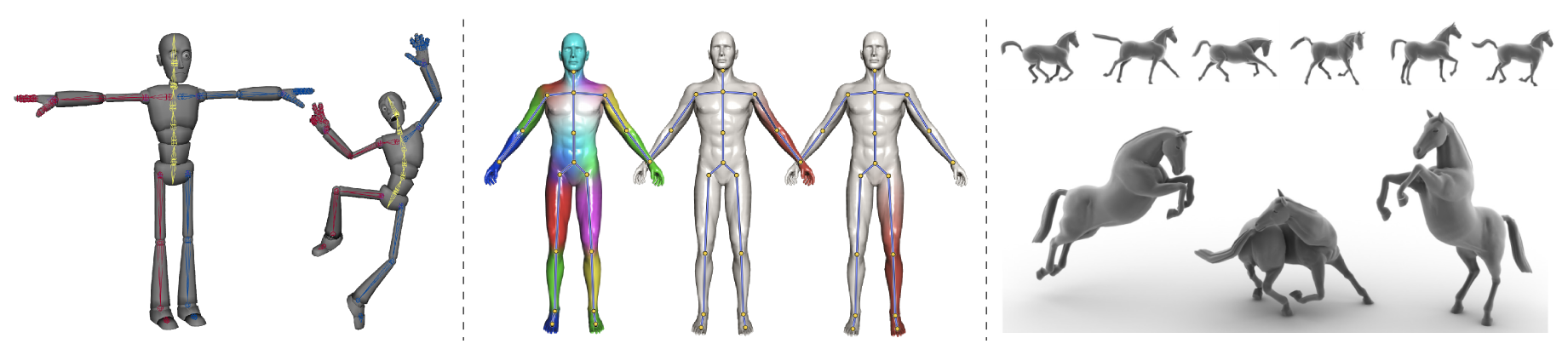
Figure 18: (a) An example of a kinematic skeleton (also called animation rig) from MAYA is used to articulate the shape from its rest-pose to a desired one. (b) Each bone (i.e. edge) of the curve skeleton is associated with skinning weights that describe how its movement affects the surface vertices [Jacobson et al. 2011]. (c) Given a set of example poses (top), it’s possible to automatically estimate skinning weights and skeletons [Schaefer and Yuksel 2007]; (bottom) this information is sufficient to extrapolate new poses.

In computer animation, posing digital characters is an essential task and there are multiple ways to achieve it. For example, we can directly manipulate the surface [Lipman et al. 2005] or use control cages [Lipman et al. 2008]. Arguably the most commonly used method is Skeletal Subspace Deformation [Lewis et al. 2000], where curve skeletons mimic the way real-world bones create deformations in our own bodies. Not only is skeletal deformation found in most 3D modeling packages but its efficient computation is so crucial that it is commonly hardware-accelerated on GPUs. In SSD, the animator specifies a kinematic skeleton for a rest-pose of the shape – like the T-pose of Figure 18-(a,left). To obtain a desired pose, a set of transformations (typically rigid) are applied in hierarchical fashion to the rest-pose skeleton. Finally, the posed shape is obtained by transferring the bone transformations onto surface vertices as shown in Figure 18-(a,right); this is achieved by performing a weighted combination of transformations. These weights are typically called skinning weights: a scalar field that encodes how much a surface region should be influenced by a particular bone (See Figure 18-b).

As the generation and skinning of kinematic skeletons is a time consuming task, a number of algorithms has addressed the problem of automating the process. For example, in [Wade and Parent 2000, Delias et al. 2007] the authors considered the problem of fitting templates of skeletons in digital human models. In [Baran and Popović 2007], the authors generalized the approach, not only considering fitting of more complex skeletons (i.e. not human), but also in the more general sense of transferring animations between different shapes. If a sequence of pre-animated meshes is given, a skeleton can be extracted with the techniques discussed in

44 skeletons:computation:grouping

and their skinning weights can be computed in a completely automated fashion [Schaefer and Yuksel 2007] as illustrated in Figure 18-c. This possibility of converting animations to the SSD framework has been demonstrated to be very effective for animation compression [De Aguiar et al. 2008]. In addition, note that the generation of kinematic skeletons and weights is not restricted to surface models, but elegantly extends to volumetric data [Gagvani and Silver 2001, Theobalt et al. 2004].

The applications of curve skeletons in animation are not limited to generating shape poses and parameters. For example, in [Lazarus and Verroust 1997], the authors employ skeletons as a parameterization domain suitable for shape blending of simple shapes. Furthermore, the performance of collision detection algorithms based on bounding volume hierarchies can be enhanced by decomposing shapes using skeletons [Li et al. 2001].

44.0.1 Geometry processing

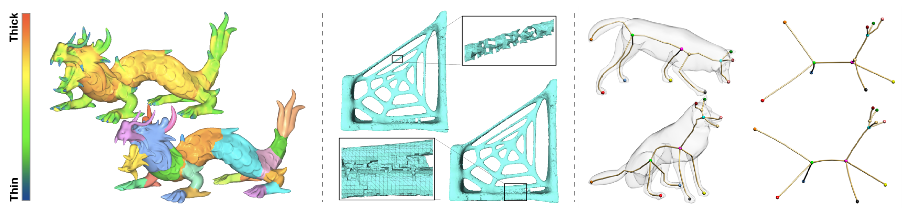
Figure 19: (a) The surface to skeleton correspondences allow to define a radius function (top) onto the surface which can be used to segment the shape (bottom) [Au et al. 2008]. (b) The compact topological representation of the curve skeleton is used to drive a topology fixing process [Zhou et al. 2007]. (c) Multi-dimensional scaling can be efficiently performed on the skeleton, resulting in stretched out limbs which facilitate the task of left/right disambiguation commonly found in articulated shape correspondence [Au et al. 2010].

Curve skeletons have broad applications in the modeling and analysis of geometry. Their branches are part-aware and associated with important shape features, allowing the development of efficient segmentation algorithms for simple human-like objects [Xiao et al. 2003, Werghi et al. 2006], as well as for shapes with more complex structure [Reniers and Telea 2007, Tierny et al. 2007, Au et al. 2008]. Their ability to compactly represent topology has been exploited to automatically correct topological problems in isosurfaces of implicit functions [Wood et al. 2004] and low quality surface models [Zhou et al. 2007]. Its approximate reconstruction properties have been exploited for the modeling of organic shapes [Angelidis et al. 2002, Ji et al. 2010] as well as for the correction of geometry in acquired data [Tagliasacchi et al. 2009, Cao et al. 2010, Zheng et al. 2010]. Curve skeletons are also very useful to address the correspondence problem particularly for datasets consisting of shapes characterized by many protrusions. Their compactness allows to greatly reduce the input size of what is essentially a combinatorial problem.

Shape correspondence

Shape correspondence addresses the problem of identifying meaningful relationships between elements of two shapes. A large variety of methods solve the problem by directly analyzing the shape geometry [Tangelder and Veltkamp 2008, van Kaick et al. 2010]. On the other hand, curve skeletons compactly represent a shape as the graph of its components, their relationship and, in some scenarios, a rough description of their geometry [Biasotti et al. 2000a]. Consequently, an alternative approach to establish a correspondence between shapes can be obtained by comparing their graphs [Hilaga et al. 2001]. This is advantageous because the size of graph is usually much smaller than the size of the surface (i.e. number of triangles) or volumetric representations (i.e. number of voxels), allowing more computationally-expensive algorithms to run in reasonable time. In addition, when shapes exhibit large variation in poses and surface details, a graph representation better captures the shape’s overall structure than local geometric measures (e.g. curvature).

A possible way to compare two graphs is to identify the maximal common subgraph, but this problem is NP-hard. Alternative methods employ graph edit distances – by measuring the cost of transforming one graph into the other by simple editing operations. Although this is known to be an NP-hard problem [Zhang et al. 1996], there exist heuristic solutions (e.g. the graph often needs to be converted into an acyclic one) based on graph editing operations both in 2D [Sebastian et al. 2004] and 3D [Biasotti et al. 2006]. A different way to approach the problem is by noting that the spectral decomposition of the graph’s adjacency matrix contains much information about the topology of a graph [Siddiqi et al. 1999, Sundar et al. 2003]. As the eigen-decomposition typically captures global topological information about the graph, algorithms in this class typically proceed in a coarse to fine manner. For this reason the skeletal graph needs to be not only cycle free but also capable of expressing the natural hierarchical structure of the shape. Other more direct solutions compute correspondences by directly comparing sets of skeletal nodes in either a hierarchical way by means of a set of heuristics [Hilaga et al. 2001], or by a carefully designed voting scheme [Au et al. 2010].

44.0.2 Medical shape analysis

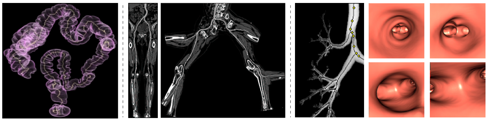
Figure 20: Examples of the use of curve skeletons in medical applications. (a) The skeletal centreline of the colon is extracted to allow virtual colonoscopy [Wan et al. 2001] or its unwinding [Silver and Gagvani 2002]. (b) The skeleton of the vessel structure is used to perform planar reformation to visualize its untangled structure [Kanitsar et al. 2003]. (c) The centreline automatically generates flight paths for virtual bronchoscopy [Perchet et al. 2004].

In the medical domain, curve skeletons are well suited to describe anatomical structures that have characteristic tubular shapes like vessels, nerves and elongated muscles [Nystrom et al. 2001, Fridman et al. 2004]. The compactness of the representation allows to efficiently perform computational tasks like registration of partially overlapped vessel images [Aylward et al. 2003] and the flattening of their three dimensional structure to a plane [Kanitsar et al. 2003]. Furthermore, the encoded local volumetric information can help in the detection of abnormalities in vascular structures, like stenosis [Sorantin et al. 2002] and aneurisms [Straka et al. 2004]. Skeletons satisfying centeredness and reliability are also particularly important in medical applications. Indeed, in virtual navigation [Wan et al. 2001], it is essential that the physician is able to examine the full internal surface of an organ [He et al. 2001]. In this context, appropriately extracted curve skeletons can be used to generate camera fly-through paths for the inspection of the intestine [Hong et al. 1997, Wan et al. 2002], lungs [Perchet et al. 2004] and blood vessels [Bartz et al. 1999]. In addition, when the structure is so tangled that even a virtual navigation would be uninformative, the skeleton can be used to straighten the organ to a linear structure which can be more easily analyzed [Silver and Gagvani 2002].

45 Conclusions

In this report, I presented a detailed overview of skeletal representations as an alternative (or addition) to boundary or volumetric representations for shape processing.

First, I introduced the idea of medial skeletons as a way of capturing redundancy and obtaining local axial representations. I discussed different possible interpretations, several classes of algorithms for its computation, its limitations in terms of stability, along with several ways to tackle this problem. For surface-based representations, I justified how Voronoi-based medial axis extraction methods offer clear advantages with regards to their competitors: not only do they offer theoretical convergence guarantees under appropriate sampling, but efficient and robust libraries for three dimensional voronoi computation are freely available as well. Although, only for two dimensional shapes, medial skeletons result in curvilinear structures, I illustrated how the medial surfaces associated with three dimensional solids contain useful information exploitable in many applications.

The necessity for a simpler curvilinear structure for three dimensional shapes stirred the discussion toward curve skeletons. While there is no unique definition for curve skeletons, I concisely described the properties that these curvilinear representations are commonly required to have. I then presented several classes of algorithms for skeletonization of solid shapes, focusing on those algorithms that operate on boundary representations. I highlighted how contraction methods currently represent the state of the art for skeletonization, because they can efficiently extract skeletons from low quality and possibly noisy surface representations without needing any domain-specific information. I concluded my discussion by describing a number of applications of curve skeletons and highlighting their abilities in describing shape from various applicative fields.

Appendix

Maximal inscribed ball

Let $\mathcal{O}$ be a closed connected set in $\mathds{R}^{n}$. A closed ball $B\subset\mathds{R}^{n}$ is called maximal inscribed ball in $\mathcal{O}$ if $B\subset\mathcal{O}$ and there does not exist another ball $B^{\prime}\neq B$ such that $B\subset B^{\prime}\subset S$.

Voronoi diagram

Given a finite set of points $S$ in $\mathds{R}^{k}$, for each point $p$ in $\mathds{R}^{k}$ there is at least one point in $S$ closest to $p$. a point $p$ may be equally close to two or more points in $S$. For each point in $S$ its Voronoi cell is defined as the subset of $R^{k}$ of points closest to it than to any other point in $S$. The union of Voronoi cells of all points in $S$ is called the Voronoi Diagram of the set $S$. For $n=|S|$ and $k=3$ the complexity is $\Uptheta(n^{2})$, but when points are well distributed on a smooth surface the complexity has been shown to reduce to $O(n\log n)$ [Attali et al. 2003].

Voronoi pole

Given a finite set of points S in $\mathds{R}^{k}$ and its Voronoi diagram, each sample point $p$ is associated with a convex Voronoi polyhedron. The vertices on the polyhedron on the two sides of the boundary which are further from $p$ are the Voronoi poles of $p$. Note that there are at most $2n$ poles for a sample of size $n$.

Local feature size

The local feature size $\text{LFS}(x)$ is the minimum Euclidean distance from any point x to any point of the medial axis.

Delta sampling (i.e. uniform sampling)

A sample $P$ of $\mathcal{S}$ is a $\delta$-sample if no point $p\in\mathcal{S}$ is further than $\delta$ from $P$.

Epsilon sampling (i.e. adaptive sampling)

A sample $P$ of $\mathcal{S}$ is an $\epsilon$-sample if no point $p\in\mathcal{S}$ is farther than $r\cdot LFS(p)$ from $\mathcal{M}$.

References

- [\citenameAmenta and Bern 1998] Amenta, N., and Bern, M. 1998. Surface reconstruction by voronoi filtering. In Proceedings of the ACM Symposium on Computational geometry, ACM, 39–48.
- [\citenameAmenta et al. 1998a] Amenta, N., Bern, M., and Eppstein, D. 1998. The crust and the beta-skeleton: combinatorial curve reconstruction. Graphical models and image processing 60, 2, 125–135.
- [\citenameAmenta et al. 1998b] Amenta, N., Bern, M., and Kamvysselis, M. 1998. A new Voronoi-based surface reconstruction algorithm. ACM Transactions on Graphics (Proceedings of SIGGRAPH), 415–421.
- [\citenameAmenta et al. 2000] Amenta, N., Choi, S., and Kolluri, R. K. 2000. The power crust, unions of balls, and the medial axis transform. Computational Geometry: Theory and Applications 19, 127–153.
- [\citenameAmenta et al. 2001] Amenta, N., Choi, S., and Kolluri, R. K. 2001. The power crust. In Proceedings of the ACM Symposium on Solid Modeling and Applications, ACM, 249–266.
- [\citenameAngelidis and Cani 2002] Angelidis, A., and Cani, M. 2002. Adaptive implicit modeling using subdivision curves and surfaces as skeletons. In Proceedings of the ACM Symposium on Solid Modeling and Applications, ACM, 45–52.
- [\citenameAngelidis et al. 2002] Angelidis, A., Jepp, P., and Cani, M. 2002. Implicit modeling with skeleton curves: Controlled blending in contact situations. In Proceedings of the IEEE Conference on Shape Modeling and Applications, IEEE Computer Society.
- [\citenameAnguelov et al. 2004] Anguelov, D., Koller, D., Pang, H., Srinivasan, P., and Thrun, S. 2004. Recovering articulated object models from 3d range data. In Proceedings of the 20th conference on Uncertainty in artificial intelligence, AUAI Press, 18–26.
- [\citenameAttali and Montanvert 1996] Attali, D., and Montanvert, A. 1996. Modeling noise for a better simplification of skeletons. In Proceedings of the International Conference on Image Processing, IEEE Computer Society, 13–16.
- [\citenameAttali and Montanvert 1997] Attali, D., and Montanvert, A. 1997. Computing and simplifying 2D and 3D continuous skeletons. Computer Vision and Image Understanding 67, 3, 261 – 273.
- [\citenameAttali et al. 2003] Attali, D., Boissonnat, J. D., and Lieutier, A. 2003. Complexity of the Delaunay triangulation of points on surfaces the smooth case. In Proceedings of the ACM Symposium on Computational Geometry, ACM, 201–210.
- [\citenameAttali et al. 2009] Attali, D., Boissonnat, J. D., and Edelsbrunner, H. 2009. Stability and computation of medial axes a state-of-the-art report. Mathematical foundations of scientific visualization, computer graphics, and massive data exploration, 109–125.
- [\citenameAu et al. 2008] Au, O. K.-C., Tai, C.-L., Chu, H.-K., Cohen-Or, D., and Lee, T.-Y. 2008. Skeleton extraction by mesh contraction. ACM Transactions on Graphics (Proceedings of SIGGRAPH) 27, 3, 44(1–10).
- [\citenameAu et al. 2010] Au, O. K.-C., Tai, C.-L., Cohen-Or, D., Zheng, Y., and Fu, H. 2010. Electors voting for fast automatic shape correspondence. Computer Graphics Forum (Proceedings of Eurographics) 29, 2, 645–654.
- [\citenameAylward et al. 2003] Aylward, S., Jomier, J., Weeks, S., and Bullitt, E. 2003. Registration and analysis of vascular images. International Journal of Computer Vision 55, 2, 123–138.
- [\citenameBaran and Popović 2007] Baran, I., and Popović, J. 2007. Automatic rigging and animation of 3D characters. ACM Transactions on Graphics (Proceedings of SIGGRAPH) 26, 3, 72(1–8).
- [\citenameBartz et al. 1999] Bartz, D., Straßer, W., Skalej, M., and Welte, D. 1999. Interactive exploration of extra and intracranial blood vessels (case study). In Proceedings of the IEEE Conference on Visualization, IEEE Computer Society, 389–392.
- [\citenameBiasotti et al. 2000a] Biasotti, S., Falcidieno, B., and Spagnuolo, M. 2000. Extended reeb graphs for surface understanding and description. In Discrete Geometry for Computer Imagery, Springer, 185–197.
- [\citenameBiasotti et al. 2000b] Biasotti, S., Falcidieno, B., and Spagnuolo, M. 2000. Extended reeb graphs for surface understanding and description. In International Conference on Discrete Geometry for Computer Imagery, Springer, 185–197.
- [\citenameBiasotti et al. 2003] Biasotti, S., Marini, S., Mortara, M., and Patané, G. 2003. An overview on properties and efficacy of topological skeletons in shape modelling. In Proceedings of the IEEE Conference on Shape Modeling and Applications, IEEE Computer Society, 245–254.
- [\citenameBiasotti et al. 2006] Biasotti, S., Marini, S., Spagnuolo, M., and Falcidieno, B. 2006. Sub-part correspondence by structural descriptors of 3D shapes. Computer-Aided Design 38, 9, 1002–1019.
- [\citenameBlanding et al. 2000] Blanding, R. L., Turkiyyah, G. M., Storti, D. W., and Ganter, M. A. 2000. Skeleton-based three-dimensional geometric morphing. Computational Geometry 15, 1-3, 129–148.
- [\citenameBloomenthal and Lim 1999] Bloomenthal, J., and Lim, C. 1999. Skeletal methods of shape manipulation. In Proceedings of the ACM Symposium on Solid Modeling and Applications, IEEE Computer Society, 44–47.
- [\citenameBloomenthal 2002] Bloomenthal, J. 2002. Medial-based vertex deformation. In Proceedings of the ACM/EG Symposium on Computer Animation, ACM, 147–151.
- [\citenameBlum 1967] Blum, H. 1967. A transformation for extracting new descriptors of shape. Models for the perception of speech and visual form. MIT Press.
- [\citenameBlum 1973] Blum, H. 1973. Biological shape and visual science (Part I). Journal of theoretical Biology 38, 2, 205–287.
- [\citenameBrandt and Algazi 1992] Brandt, J. W., and Algazi, V. R. 1992. Continuous skeleton computation by Voronoi diagram. CVGIP: Image Understanding 55, 329–338.
- [\citenameCao et al. 2010] Cao, J., Tagliasacchi, A., Olson, M., Zhang, H., and Su, Z. 2010. Point cloud skeletons via Laplacian based contraction. In Proceedings of the IEEE Conference on Shape Modeling and Applications, IEEE Computer Society, 187–197.
- [\citenameCazals and Giesen 2006] Cazals, F., and Giesen, J. 2006. Delaunay triangulation based surface reconstruction. Effective computational geometry for curves and surfaces, 231–276.
- [\citenameChang et al. 2004] Chang, M., Leymarie, F., and Kimia, B. 2004. 3D shape registration using regularized medial scaffolds. In Proceedings of the International Symposium on 3D Data Processing, Visualization, and Transmission (3DPVT), IEEE Computer Society, 987–994.
- [\citenameChaussard et al. 2009] Chaussard, J., Couprie, M., and Talbot, H. 2009. A discrete lambda-medial axis. In Discrete Geometry for Computer Imagery, vol. 5810 of Lecture Notes in Computer Science, Springer, 421–433.
- [\citenameChazal and Lieutier 2004] Chazal, F., and Lieutier, A. 2004. Stability and homotopy of a subset of the medial axis. In Proceedings of the ACM Symposium on Solid Modeling and Applications, ACM, 243–248.
- [\citenameChazal and Lieutier 2005a] Chazal, F., and Lieutier, A. 2005. Weak feature size and persistent homology: computing homology of solids in from noisy data samples. In Proceedings of the ACM Symposium on Computational Geometry, ACM, 255–262.
- [\citenameChazal and Lieutier 2005b] Chazal, F., and Lieutier, A. 2005. The medial axis. Graphical Models 67, 304–331.
- [\citenameChuang et al. 2004] Chuang, J.-H., Ahuja, N., Lin, C.-C., Tsai, C.-H., and Chen, C.-H. 2004. A potential-based generalized cylinder representation. Computers and Graphics 28, 6, 907–918.
- [\citenameCornea et al. 2007] Cornea, N. D., Min, P., and Silver, D. 2007. Curve-skeleton properties, applications, and algorithms. IEEE Transactions on Visualization and Computer Graphics 13, 3, 530–548.
- [\citenameCulver et al. 2004] Culver, T., Keyser, J., and Manocha, D. 2004. Exact computation of the medial axis of a polyhedron. Computer Aided Geometric Design 21, 1, 65–98.
- [\citenameDe Aguiar et al. 2008] De Aguiar, E., Theobalt, C., Thrun, S., and Seidel, H. 2008. Automatic conversion of mesh animations into skeleton-based animations. Computer Graphics Forum (Proceedings of Eurographics) 27, 2, 389–397.
- [\citenameDelias et al. 2007] Delias, F., Moccozet, L., Magnenat-Thalmann, N., Mortara, M., Patane, G., Spagnuolo, M., and Falcidieno, B. 2007. Knowledge-based extraction of control skeletons for animation. In Proceedings of the IEEE Conference on Shape Modeling and Applications, IEEE Computer Society, 51–60.
- [\citenameDey and Sun 2006] Dey, T., and Sun, J. 2006. Defining and computing curve-skeletons with medial geodesic function. Computer Graphics Forum (Proceedings of the ACM/EG Symposium on Geometry Processing), 143–152.
- [\citenameDey and Zhao 2004] Dey, T., and Zhao, W. 2004. Approximate medial axis as a voronoi subcomplex. Computer-Aided Design 36, 2, 195–202.
- [\citenamedi Baja and Thiel 1996] di Baja, S., and Thiel, E. 1996. Skeletonization algorithm running on path-based distance maps. Image and Vision Computing 14, 1, 47–57.
- [\citenameEdelsbrunner and Mücke 1994] Edelsbrunner, H., and Mücke, E. P. 1994. Three-dimensional alpha shapes. ACM Transactions on Graphics (TOG) 13, 43–72.
- [\citenameFridman et al. 2004] Fridman, Y., Pizer, S., Aylward, S., and Bullitt, E. 2004. Extracting branching tubular object geometry via cores. Medical Image Analysis 8, 3, 169–176.
- [\citenameGagvani and Silver 2001] Gagvani, N., and Silver, D. 2001. Animating volumetric models. Graphical Models 63, 443–458.
- [\citenameGiblin and Brassett 1985] Giblin, P. J., and Brassett, S. A. 1985. Local symmetry of plane curves. The American Mathematical Monthly, 689–707.
- [\citenameGiblin and Kimia 2004] Giblin, P., and Kimia, B. 2004. A formal classification of 3D medial axis points and their local geometry. IEEE Transactions on Pattern Analysis and Machine Intelligence, 238–251.
- [\citenameGiesen et al. 2009] Giesen, J., Miklos, B., Pauly, M., and Wormser, C. 2009. The scale axis transform. In Proceedings of the ACM Symposium on Computational Geometry, ACM, 106–115.
- [\citenameHassouna and Farag 2008] Hassouna, M., and Farag, A. 2008. Variational curve skeletons using gradient vector flow. IEEE Transactions on Pattern Analysis and Machine Intelligence, 2257–2274.
- [\citenameHe et al. 2001] He, T., Hong, L., Chen, D., and Liang, Z. 2001. Reliable path for virtual endoscopy: ensuring complete examination of human organs. IEEE Transactions on Visualization and Computer Graphics, 333–342.
- [\citenameHeld 2001] Held, M. 2001. Vroni: An engineering approach to the reliable and efficient computation of Voronoi diagrams of points and line segments. Computational Geometry: Theory and Applications 18, 2, 95–123.
- [\citenameHilaga et al. 2001] Hilaga, M., Shinagawa, Y., Kohmura, T., and Kunii, T. L. 2001. Topology matching for fully automatic similarity estimation of 3D shapes. ACM Transactions on Graphics (Proceedings of SIGGRAPH), 203–212.
- [\citenameHisada et al. 2002] Hisada, M., Belyaev, A., and Kunii, T. 2002. A skeleton-based approach for detection of perceptually salient features on polygonal surfaces. Computer Graphics Forum (Proceedings of Eurographics) 21, 4, 689–700.
- [\citenameHong et al. 1997] Hong, L., Muraki, S., Kaufman, A., Bartz, D., and He, T. 1997. Virtual voyage: Interactive navigation in the human colon. ACM Transactions on Graphics (Proceedings of SIGGRAPH), 27–34.
- [\citenameHubbard 1996] Hubbard, P. 1996. Approximating polyhedra with spheres for time-critical collision detection. ACM Transactions on Graphics (TOG) 15, 3, 179–210.
- [\citenameJacobson et al. 2011] Jacobson, A., Baran, I., Popović, J., and Sorkine, O. 2011. Bounded biharmonic weights for real-time deformation. ACM Transactions on Graphics (Proceedings of SIGGRAPH) 30, 4, 78:1–78:8.
- [\citenameJi et al. 2010] Ji, Z., Liu, L., and Wang, Y. 2010. B-mesh: A modeling system for base meshes of 3D articulated shapes. Computer Graphics Forum (Proceedings of Pacific Graphics) 29, 7, 2169–2178.
- [\citenameKanitsar et al. 2003] Kanitsar, A., Wegenkittl, R., Fleischmann, D., and Groller, M. 2003. Advanced curved planar reformation: Flattening of vascular structures. Proceedings of the IEEE Conference on Visualization, 43–50.
- [\citenameKatz and Tal 2003] Katz, S., and Tal, A. 2003. Hierarchical mesh decomposition using fuzzy clustering and cuts. ACM Transactions on Graphics (Proceedings of SIGGRAPH), 954–961.
- [\citenameKimia et al. 1995] Kimia, B., Tannenbaum, A., and Zucker, S. 1995. Shapes, shocks, and deformations I: the components of two-dimensional shape and the reaction-diffusion space. International Journal of Computer Vision 15, 3, 189–224.
- [\citenameLazarus and Verroust 1997] Lazarus, F., and Verroust, A. 1997. Metamorphosis of cylinder-like objects. The journal of visualization and computer animation 8, 3, 131–146.
- [\citenameLazarus and Verroust 1999] Lazarus, F., and Verroust, A. 1999. Level set diagrams of polyhedral objects. In Proceedings of the ACM Symposium on Solid Modeling and Applications, ACM, 130–140.
- [\citenameLee et al. 1994] Lee, T., Kashyap, R., and Chu, C. 1994. Building skeleton models via 3D medial surface/axis thinning algorithms. CVGIP: Graphical Model and Image Processing 56, 6, 462–478.
- [\citenameLee 1982] Lee, D. 1982. Medial axis transformation of a planar shape. IEEE Transactions on Pattern Analysis and Machine Intelligence, 4, 363–369.
- [\citenameLewis et al. 2000] Lewis, J. P., Cordner, M., and Fong, N. 2000. Pose space deformation: a unified approach to shape interpolation and skeleton-driven deformation. ACM Transactions on Graphics (Proceedings of SIGGRAPH), 165–172.
- [\citenameLi et al. 2001] Li, X., Woon, T., Tan, T., and Huang, Z. 2001. Decomposing polygon meshes for interactive applications. In Proceedings of the Symposium on Interactive 3D Graphics, ACM, 35–42.
- [\citenameLien et al. 2006] Lien, J., Keyser, J., and Amato, N. 2006. Simultaneous shape decomposition and skeletonization. In Proceedings of the ACM Symposium on Solid and Physical Modeling, ACM, 219–228.
- [\citenameLieutier 2003] Lieutier, A. 2003. Any open bounded subset of rn has the same homotopy type than its medial axis. In Proceedings of the ACM Symposium on Solid Modeling and Applications, ACM, 65–75.
- [\citenameLipman et al. 2005] Lipman, Y., Sorkine, O., Levin, D., and Cohen-Or, D. 2005. Linear rotation-invariant coordinates for meshes. ACM Transactions on Graphics (TOG) 24, 3, 479–487.
- [\citenameLipman et al. 2008] Lipman, Y., Levin, D., and Cohen-Or, D. 2008. Green coordinates. ACM Transactions on Graphics (Proceedings of SIGGRAPH), 78:1–78:10.
- [\citenameMather 1983] Mather, J. 1983. Distance from a sub-manifold in Euclidean space. In Proceedings of Symposia in Pure Mathematics, Citeseer.
- [\citenameMiklos et al. 2010] Miklos, B., Giesen, J., and Pauly, M. 2010. Discrete scale axis representations for 3d geometry. ACM Transactions on Graphics (TOG) 29, 4, 101.
- [\citenameMortara et al. 2003] Mortara, M., Patané, G., Spagnuolo, M., Falcidieno, B., and Rossignac, J. 2003. Blowing bubbles for multi-scale analysis and decomposition of triangle meshes. Algorithmica 38, 1, 227–248.
- [\citenameMusuvathy et al. 2011] Musuvathy, S., Cohen, E., and Damon, J. 2011. Computing medial axes of generic 3D regions bounded by B-spline surfaces. Computer-Aided Design (to appear).
- [\citenameNäf et al. 1997] Näf, M., Szekely, G., Kikinis, R., Shenton, M., and Kübler, O. 1997. 3D Voronoi skeletons and their usage for the characterization and recognition of 3D organ shape. Computer Vision and Image Understanding 66, 2, 147–161.
- [\citenameNatali et al. 2011] Natali, M., Biasotti, S., Patanč, G., and Falcidieno, B. 2011. Graph-based representations of point clouds. Graphical Models (to appear).
- [\citenameNystrom et al. 2001] Nystrom, I., di Baja, G., and Svensson, S. 2001. Representing volumetric vascular structures using curve skeletons. In Proceedings of the International conference on Image Analysis and Processing, IEEE Computer Society, 495–500.
- [\citenamePaik et al. 1998] Paik, D., Beaulieu, C., Jeffrey, R., Rubin, G., and Napel, S. 1998. Automated flight path planning for virtual endoscopy. Medical Physics 25, 629.
- [\citenamePalágyi and Kuba 1999] Palágyi, K., and Kuba, A. 1999. A parallel 3D 12-subiteration thinning algorithm. Graphical Models and Image Processing 61, 4, 199–221.
- [\citenamePerchet et al. 2004] Perchet, D., Fetita, C., and Prêteux, F. 2004. Advanced navigation tools for virtual bronchoscopy. In Proceedings of SPIE Conference on Image Processing: Algorithms and Systems III, vol. 5298, Citeseer, 147–158.
- [\citenamePizer et al. 2000] Pizer, S., Thall, A., and Chen, D. 2000. M-reps: A new object representation for graphics. Tech. Rep. TR99-030, University of North Carolina, Chapel Hill, NC, 17.
- [\citenamePizer et al. 2003] Pizer, S., Fletcher, P., Joshi, S., Thall, A., Chen, J., Fridman, Y., Fritsch, D., Gash, A., Glotzer, J., Jiroutek, M., et al. 2003. Deformable m-reps for 3D medical image segmentation. International Journal of Computer Vision 55, 2, 85–106.
- [\citenamePizer et al. 2011] Pizer, S., Jung, S., Goswami, D., Zhao, X., Chaudhuri, R., Damon, J., Huckemann, S., and Marron, J. 2011. Nested sphere statistics of skeletal models. In Proceedings of the Dagstuhl workshop on innovations for shape analysis: models and algorithms, vol. (to appear), Citeseer.
- [\citenameReniers and Telea 2007] Reniers, D., and Telea, A. 2007. Skeleton based hierarchical shape segmentation. In Proceedings of the IEEE Conference on Shape Modeling and Applications, IEEE Computer Society, 179–188.
- [\citenameRuuth and Wetton 2003] Ruuth, S., and Wetton, B. 2003. A simple scheme for volume-preserving motion by mean curvature. Journal of Scientific Computing 19, 1, 373–384.
- [\citenameSchaefer and Yuksel 2007] Schaefer, S., and Yuksel, C. 2007. Example-based skeleton extraction. Computer Graphics Forum (Proceedings of the ACM/EG Symposium on Geometry Processing), 153–162.
- [\citenameSebastian et al. 2004] Sebastian, T., Klein, P., and Kimia, B. 2004. Recognition of shapes by editing their shock graphs. IEEE Transactions on Pattern Analysis and Machine Intelligence 26, 5, 550–571.
- [\citenameSethian 1996] Sethian, J. 1996. A fast marching level set method for monotonically advancing fronts. Proceedings of the National Academy of Sciences 93, 4, 1591.
- [\citenameShah 2005] Shah, J. 2005. Gray skeletons and segmentation of shapes. Computer Vision and Image Understanding 99, 1, 96–109.
- [\citenameShaham et al. 2004] Shaham, A., Shamir, A., and Cohen-Or, D. 2004. Medial axis based solid representation. In Proceedings of the ACM Symposium on Solid Modeling and Applications, IEEE Computer Society, 37–44.
- [\citenameShamir 2008] Shamir, A. 2008. A survey on mesh segmentation techniques. Computer Graphics Forum 27, 6, 1539–1556.
- [\citenameShapira et al. 2008] Shapira, L., Shamir, A., and Cohen-Or, D. 2008. Consistent mesh partitioning and skeletonization using the shape diameter function. The Visual Computer 24, 4, 249–259.
- [\citenameShinagawa et al. 1991] Shinagawa, Y., Kunii, T. L., and Kergosien, Y. L. 1991. Surface coding based on morse theory. IEEE Computer Graphics and Applications 11, 66–78.
- [\citenameSiddiqi et al. 1999] Siddiqi, K., Shokoufandeh, A., Dickinson, S., and Zucker, S. 1999. Shock graphs and shape matching. International Journal of Computer Vision 35, 1, 13–32.
- [\citenameSiddiqi et al. 2002] Siddiqi, K., Bouix, S., Tannenbaum, A., and Zucker, S. 2002. Hamilton-jacobi skeletons. International Journal of Computer Vision 48, 3, 215–231.
- [\citenameSilver and Gagvani 2002] Silver, D., and Gagvani, N. 2002. Unwinding the colon. In Medicine Meets Virtual Reality, vol. 9, Citeseer.
- [\citenameSorantin et al. 2002] Sorantin, E., Halmai, C., Erdohelyi, B., Palágyi, K., Nyúl, L., Ollé, K., Geiger, B., Lindbichler, F., Friedrich, G., and Kiesler, K. 2002. Spiral ct based assessment of tracheal stenoses using 3D skeletonization. IEEE Transactions on Medical Imaging 21, 3, 263–273.
- [\citenameStorti et al. 1997] Storti, D., Turkiyyah, G., Ganter, M., Lim, C., and Stal, D. 1997. Skeleton-based modeling operations on solids. In Proceedings of the ACM Symposium on Solid Modeling and Applications, ACM, 141–154.
- [\citenameStraka et al. 2004] Straka, M., Červeňanskỳ, M., La Cruz, A., Köchl, A., Šrámek, M., Gröller, E., and Fleischmann, D. 2004. The vesselglyph: Focus & context visualization in ct-angiography. In Proceedings of the IEEE Conference on Visualization, IEEE Computer Society, 385–392.
- [\citenameStyner et al. 2003] Styner, M., Gerig, G., Joshi, S., and Pizer, S. 2003. Automatic and robust computation of 3d medial models incorporating object variability. International Journal of Computer Vision 55, 2, 107–122.
- [\citenameSud et al. 2005] Sud, A., Foskey, M., and Manocha, D. 2005. Homotopy-preserving medial axis simplification. In Proceedings of the ACM Symposium on Solid and Physical Modeling, ACM, 39–50.
- [\citenameSun and Sherrah 1997] Sun, C., and Sherrah, J. 1997. 3D symmetry detection using the extended Gaussian image. IEEE Transactions on Pattern Analysis and Machine Intelligence, 164–168.
- [\citenameSundar et al. 2003] Sundar, H., Silver, D., Gagvani, N., and Dickinson, S. 2003. Skeleton based shape matching and retrieval. In Proceedings of the IEEE Conference on Shape Modeling and Applications, IEEE Computer Society, 130–139.
- [\citenameTagliasacchi et al. 2009] Tagliasacchi, A., Zhang, H., and Cohen-Or, D. 2009. Curve skeleton extraction from incomplete point cloud. ACM Transactions on Graphics, (Proceedings SIGGRAPH 2009) 28, 3, 71:1–71:9.
- [\citenameTagliasacchi et al. 2011] Tagliasacchi, A., Olson, M., Zhang, H., Hamarneh, G., and Cohen-Or, D. 2011. VASE: Volume-Aware Surface Evolution for surface reconstruction from incomplete point clouds. Computer Graphics Forum (Proceedings of the ACM/EG Symposium on Geometry Processing) 30, 5, 1563–1571.
- [\citenameTam and Heidrich 2003] Tam, R., and Heidrich, W. 2003. Shape simplification based on the medial axis transform. In Proceedings of the IEEE Conference on Visualization, IEEE Computer Society, 63–71.
- [\citenameTangelder and Veltkamp 2008] Tangelder, J., and Veltkamp, R. 2008. A survey of content based 3D shape retrieval methods. Multimedia Tools and Applications 39, 3, 441–471.
- [\citenameTchon et al. 2003] Tchon, K., Khachan, M., Guibault, F., and Camarero, R. 2003. Constructing anisotropic geometric metrics using octrees and skeletons. In International Meshing Roundtable, Citeseer.
- [\citenameTheobalt et al. 2004] Theobalt, C., De Aguiar, E., Magnor, M., Theisel, H., and Seidel, H. 2004. Marker-free kinematic skeleton estimation from sequences of volume data. In Proceedings of the ACM Symposium on Virtual Reality Software and Technology, ACM, 57–64.
- [\citenameTierny et al. 2007] Tierny, J., Vandeborre, J., and Daoudi, M. 2007. Topology driven 3D mesh hierarchical segmentation. In Proceedings of the IEEE Conference on Shape Modeling and Applications, IEEE Computer Society, 215–220.
- [\citenameTzoumas 2011] Tzoumas, G. M. 2011. Exact medial axis of quadratic NURBS curves. Computational Geometry: Theory and Applications (to appear).
- [\citenamevan Kaick et al. 2010] van Kaick, O., Zhang, H., Hamarneh, G., and Cohen-Or, D. 2010. A survey on shape correspondence. Computer Graphics Forum (Eurographics STAR report).
- [\citenameWade and Parent 2000] Wade, L., and Parent, R. 2000. Fast, fully-automated generation of control skeletons for use in animation. In Proceedings of Computer Animation, IEEE Computer Society, 164–169.
- [\citenameWan et al. 2001] Wan, M., Dachille, F., and Kaufman, A. 2001. Distance-field based skeletons for virtual navigation. In Proceedings of the IEEE Conference on Visualization, IEEE Computer Society, 246.
- [\citenameWan et al. 2002] Wan, M., Liang, Z., Ke, Q., Hong, L., Bitter, I., and Kaufman, A. 2002. Automatic centerline extraction for virtual colonoscopy. IEEE Transactions on Medical Imaging 21, 12, 1450–1460.
- [\citenameWang and Lee 2008] Wang, Y., and Lee, T. 2008. Curve-skeleton extraction using iterative least squares optimization. IEEE Transactions on Visualization and Computer Graphics 14, 4, 926–936.
- [\citenameWard and Hamarneh 2009] Ward, A., and Hamarneh, G. 2009. The groupwise medial axis transform for fuzzy skeletonization and pruning. IEEE Transactions on Pattern Analysis and Machine Intelligence, 1084–1096.
- [\citenameWerghi et al. 2006] Werghi, N., Xiao, Y., and Siebert, J. 2006. A functional-based segmentation of human body scans in arbitrary postures. IEEE Transactions on Systems, Man, and Cybernetics, Part B: Cybernetics 36, 1, 153–165.
- [\citenameWood et al. 2004] Wood, Z., Hoppe, H., Desbrun, M., and Schroder, P. 2004. Removing excess topology from isosurfaces. ACM Transactions on Graphics (TOG) 23, 2, 190–208.
- [\citenameXiao et al. 2003] Xiao, Y., Siebert, P., and Werghi, N. 2003. A discrete Reeb graph approach for the segmentation of human body scans. In Proceedings of the International Conference on 3D Digital Imaging and Modeling, IEEE Computer Society.
- [\citenameYoshizawa et al. 2003] Yoshizawa, S., Belyaev, A., and Seidel, H. 2003. Free-form skeleton-driven mesh deformations. In Proceedings of the ACM Symposium on Solid Modeling and Applications, ACM, 247–253.
- [\citenameYoshizawa et al. 2007] Yoshizawa, S., Belyaev, A., and Seidel, H. 2007. Skeleton-based variational mesh deformations. Computer Graphics Forum (Proceedings of Eurographics) 26, 3, 255–264.
- [\citenameZhang et al. 1996] Zhang, K., Wang, J., and Shasha, D. 1996. On the editing distance between undirected acyclic graphs. International Journal of Foundations of Computer Science 7, 1, 43–58.
- [\citenameZheng et al. 2010] Zheng, Q., Sharf, A., Tagliasacchi, A., Chen, B., Zhang, H., Sheffer, A., and Cohen-Or, D. 2010. Consensus skeleton for non-rigid space-time registration. Computer Graphics Forum (Proceedings of Eurographics) 29, 2, 635–644.
- [\citenameZhou et al. 2007] Zhou, Q., Ju, T., and Hu, S. 2007. Topology repair of solid models using skeletons. IEEE Transactions on Visualization and Computer Graphics, 675–685.
- [\citenameZhu 1999] Zhu, S. 1999. Stochastic jump-diffusion process for computing medial axes in markov random fields. IEEE Transactions on Pattern Analysis and Machine Intelligence, 1158–1169.